Unitary matrix models, free fermion ensembles, and
the giant graviton expansion

Abstract

We consider a class of matrix integrals over the unitary group $U(N)$ with an infinite set of couplings characterized by a series $f(q)=\sum_{n\geq 1}a_{n}\,q^{n}$, with $a_{n}\in\mathbb{Z}$. Such integrals arise in physics as the partition functions of free four-dimensional gauge theories on $S^{3}$ and, in particular, as the superconformal index of super Yang-Mills theory. We show that any such model can be expressed in terms of a system of free fermions in an ensemble parameterized by the infinite set of couplings. Integrating out the fermions in a given quantum state leads to a convergent expansion as a series of determinants, as shown by Borodin-Okounkov many years ago. By further averaging over the ensemble, we obtain a formula for the matrix integral as a $q$-series with successive terms suppressed by $q^{\alpha N+\beta}$ where $\alpha$, $\beta$ do not depend on $N$. This provides a matrix-model explanation of the giant graviton expansion that has been observed recently in the literature.

The influence of Don Zagier’s work on the topics discussed in this article—matrix integrals, $q$-series, sum over partitions—has been deep and wide-ranging. Don’s love and enthusiasm for interesting patterns from any area of mathematics is deeply infectious, and his ability to connect different parts of mathematics (and physics!) is a rich inspiration for many of us. This influence and inspiration underlie a great deal of the following text, and it is the author’s hope that they are, at least in part, recognizable to the reader.

1 Introduction, philosophy, and the main statement

The idea that matrix models—integrals over the space of matrices of a certain kind (hermitian/orthogonal/unitary/$\dots$)—are related to systems of fermions is an old one (see e.g. Kle (91); GM (93); DFGZJ (95) for early reviews), and has taken multiple avatars over the years. Each incarnation has brought a slightly new point of view, but the basic idea can be understood by the fact that the appropriate measure on the space of matrices is proportional to the Vandermonde polynomial of the eigenvalues of the matrix, which vanishes whenever two eigenvalues coincide. Conflating this fact with the Pauli exclusion principle—that fermionic wavefunctions vanish when two fermions collide in phase space—leads to the identification of the matrix eigenvalues with the fermions (or bilinears of the fermions). In this article we discuss another relation between a class of unitary matrix integrals and a free fermionic theory coupled linearly to an infinite set of bosonic quantum variables.

Consider the following integral over the space of $U(N)$ matrices with the invariant measure $\mathrm{d}U$, normalized such that the volume of the whole space is 1,

$$Z_{N}({\bf g})\;=\;\int_{U(N)}\,\mathrm{d}U\,\exp\biggl{(}\;\sum_{k=1}^{\infty}\,\frac{1}{k}\,g_{k}\,\mbox{Tr}\,U^{k}\,\mbox{Tr}\,U^{-k}\,\biggr{)}\,,$$ (1)

where ${\bf g}=(g_{1},g_{2},\dots)$ is an infinite-dimensional vector of variables, or coupling constants, whose choice defines the model. Such integrals arise in the algebraic problem of counting invariants of multiple matrices under simultaneous conjugation by $U(N)$ Raz (74); Pro (76); Ter (86). In physics, we encounter the very same problem as counting gauge-invariant operators in free Yang-Mills theory coupled to matter fields Sun (00); Pol (02); AMM⁺ (04). In this setting the coupling constants are given in terms of a power series as

$$g_{k}\;=\;f(q^{k})\,,\quad k=1,2,\dots\,,\qquad\text{with}\quad f(q)\;=\;\sum_{n=1}^{\infty}\,a_{n}\,q^{n}\;\in\;\mathbb{Z}[[q]]\,.$$ (2)

(Here, and below, we use the usual notation $\mathbb{Z}[[q]]$ for the ring of power series in $q$ with integer coefficients.) The resulting integral then also admits a power series expansion with integer coefficients

$$I^{f}_{N}(q)\;=\;Z_{N}\bigl{(}(f(q),f(q^{2}),\dots)\bigr{)}\;=\;\sum_{\ell\geq 0}d^{f}_{N}(\ell)\,q^{\ell}\;=\;1+\text{O}(q)\,,$$ (3)

where the integers $d_{N}(\ell)$ are given by a trace of some operator over the Hilbert space with a fixed charge $\ell$. In the simplest case it is simply the dimension of that Hilbert space or the number of invariant polynomials of a given degree $\ell$ in the algebraic problem. (The constant term in (3) is calculated by setting all the coupling constants $g_{k}=0$ in (1).)

A particularly interesting class of generating functions of the sort (3) is given by superconformal indices in four dimensional supersymmetric gauge theory, which is the generating function of the Witten index of supersymmetric (BPS) states that preserves some fraction of the supersymmetries. For each type of BPS state, $f(q)$—called the single-letter index in this context—is calculated simply only from the knowledge of the field content of the gauge theory Rom (06); KMMR (07). In order to have concrete examples, we specify the theory to be $\mathcal{N}=4$ super Yang-Mills theory, which has 16 complex supercharges. The single-letter index $f(q)$ then takes the following values for different types of BPS states

$$\begin{split}\text{$\frac{1}{2}$-BPS}:~{}\quad f(q)\;\mapsto\;f_{1/2}(q)&\;=\;q\,,\\ \text{$\frac{1}{8}$-BPS}:~{}\quad f(q)\;\mapsto\;f_{1/8}(q)&\;=\;\frac{2q}{1+q}\;=\;2q-2q^{2}+2q^{3}-2q^{4}+2q^{5}-2q^{6}+\cdots\,,\\ \text{$\frac{1}{16}$-BPS}:\quad f(q)\;\mapsto\;f_{1/16}(q)&\;=\;1-\frac{(1-q^{2})^{3}}{(1-q^{3})^{2}}\;=\;3q^{2}-2q^{3}-3q^{4}+6q^{5}-2q^{6}\;+\;\cdots\,.\end{split}$$ (4)

The above physics discussion about the superconformal index can be explained better and made more rigorous, but we will not do so here partly because there are nice mathematical expositions available (see e.g. SV (11)), and partly because it can be taken to be a black box which generates interesting examples illustrating the general presentation. There is, however, one important piece of physics that cannot really be made more rigorous but is central to the story, namely the profound AdS/CFT conjecture (which is really an infinite-variable generating function of conjectures). One point of philosophy that Don Zagier has taught us repeatedly through his works and expositions is that we should test good conjectures as extensively as we possibly can to make sure that it contains Truth, and that the best conjectures are beautiful and surprising and perhaps even contain an element of the outrageous.

As a whole community of string theorists can attest to, AdS/CFT, or more generally the idea of holography, has fulfilled the above criteria time and again. In situations where one has been able to make its predictions well-defined—even if not rigorous—from a mathematical point of view, it has created very beautiful and surprising mathematical structures. A very partial list of examples is: large-$N$ expansions in matrix models tH (74), Chern-Simons theory and CFT₂ (with some hindsight) Wit (89), low-dimensional string theory Wit (91); Kon (92) and Gopakumar-Vafa theory GV (99). It is the author’s belief that there are many more mathematical gems hiding within the structure of AdS/CFT, which are yet to be found. The aim of this article is to set up a dig in one particular corner.

What are we looking for?

As we mentioned above, the integer coefficients $d^{f}_{N}(\ell)$ in (3) count the index of BPS states in a four-dimensional gauge theory of charge $\ell$. They can be calculated to any required order on the computer by calculating the integral (1). (There is a more efficient method of calculation by writing the integral as a sum over partitions that we mention in the following.) From the point of view of the AdS/CFT conjecture, the integers $d^{f}_{N}(\ell)$ also count the same index of BPS states of charge $\ell$ in the dual theory of gravity in five dimensional asymptotically AdS space with Newton’s constant $G=1/N^{2}$.

Now, on the one hand, our understanding of the nature of quantum gravitational BPS states (and our ability to count them) is quite backward compared to say gauge theory, as it requires a precise definition of a quantum theory of gravity about which we know very little. On the other hand, we do have a good knowledge of classical non-linear solutions of the gravitational theory, like gravitons, D-branes, and black holes, which give rise to interesting predictions for patterns in the numbers $d^{f}_{N}(\ell)$ in different regimes of the charge $\ell$. As $N\to\infty$, gravitons are associated with states of charge $\text{O}(1)$, D-branes are associated with states of charge $\text{O}(N)$, and black holes are associated with states of charge $\text{O}(N^{2})$. The simplest predictions arise by estimating the thermodynamic entropy of the gravitational objects, which we now briefly review in turn.

Gravitons Since gravitons have small energies in units of Newton’s constant $1/N^{2}$, we can quantize them using usual methods of quantum field theory, and calculate their statistical entropy. One can therefore also calculate the index of multi-graviton states in AdS₅ space, whose generating function is AMM⁺ (04)

$$I^{f}_{\text{multi-graviton}}(q)\;=\;\prod_{k=1}^{\infty}\frac{1}{1-f(q^{k})}\,,$$ (5)

for all the BPS single-letter indices in (4). The AdS/CFT conjecture says that the number $d^{f}_{N}(\ell)$ for fixed $\ell$ should have a limit $N\to\infty$, and that the limiting value should be the index of multi-gravitons in AdS₅ space which is given by the $q^{\ell}$ coefficient of $I^{f}_{\text{multi-graviton}}(q)$. This can be proved for arbitrary $f(q)$ by a simple argument, which we review in Section 2.

Black holes Since black holes have energies comparable to $N^{2}$ we cannot quantize them by any known method, and so we cannot count their statistical entropy. However, the profound arguments of Bekenstein and Hawking in the 1970s showed that black holes carry thermodynamic entropy proportional to their horizon area and that, upon combining this fact with the Boltzmann equation, there should be a statistical entropy associated to the black hole. In our context, the $\frac{1}{16}$-BPS case is the only one where smooth black holes of finite horizon area are known GR (04), and the Bekenstein-Hawking entropy calculation leads to the prediction

$$\log d^{1/16}_{N}(\ell)\;=\;\frac{\pi N^{2/3}}{2\cdot 3^{1/6}}\;\ell^{2/3}\;+\;\text{O}(\ell^{1/3})\,,\quad\ell\to\infty\,.$$ (6)

This prediction has recently been computationally verified to large orders and then proved in the last few years CBCMM19a ; CKKN (18); BM (20); CBCMM19b ; Mur (22), and in this process some unexpected relations to number-theoretic functions have appeared CBM (20); CBCMM (20). We will not discuss black holes in more detail in this article.

D-branes and the main statement of this article The new point of the present article concerns the intermediate range of energies scaling linearly with $N$, corresponding to D-branes, which are also called giant gravitons in AdS space MST (00); HHI (00); GMT (00) in our context. Recall that the order of power series $f(q)$ is the smallest positive integer $\alpha$ such that the coefficient of $q^{\alpha}$ is non-zero. We show in Section 5 that for arbitrary $f(q)$ of order $\alpha>0$ the integral $I^{f}_{N}$ in (3) can be written as an infinite sum of power series of successively higher order,

$$\frac{I^{f}_{N}(q)}{I^{f}_{\infty}(q)}\;=\;\sum_{m=0}^{\infty}G^{(m)}_{f,N}(q)\,,\qquad G^{(m)}_{f,N}(q)\;\in\;q^{\alpha mN+\beta(m)}\,\mathbb{Z}[[q]]\,.$$ (7)

This type of formula was numerically observed recently in AI (19); Ima (21) for the superconformal index, and in GL (21) for a class of examples with multiple charges where one of the charges scales as $N$ and the other charges are fixed. The formula is then interpreted holographically in these interesting papers, with the $m^{\text{th}}$ term in (7) identified with the index of $m$ giant gravitons in the dual AdS space. In AI (19); Ima (21) this identification is based on an explicit calculation of the index of wrapped D-branes in AdS space for the first few values of $m$. In GL (21) it is based on the calculation of determinant operators of large powers of one matrix perturbed by other matrices BHK (02); BHLN (02) and by using the fact that giant gravitons are determinant operators in the gauge theory BBNS (02); CJR (02); Ber (04).

Our method and results In the present article we work purely with the matrix integral discussed above. We give an explicit formula in Section 5 for $G^{(m)}_{f,N}(q)$ as a certain integral transform of a determinant of a $m\times m$ matrix. The basic idea in physics language is well-known. Consider a theory of a complex massive fermion with a quartic interaction. This can be written as a non-interacting (or free) fermion theory coupled to a boson, using the Hubbard-Stratonovich (H-S) transformation. Integrating out the fermions leads to a functional determinant over the Grassman fields, and the original partition function is obtained by further averaging over the boson with a Gaussian weight. Here we have an infinite set of Grassmann variables, which is equivalent to a two-dimensional chiral fermionic field. We rewrite our integral (1) as the average $Z_{N}({\bf g})=\bigl{\langle}\widetilde{Z}_{N}\bigr{\rangle}_{\bf g}$ over the infinite set of couplings ${\bf t}$ of an auxiliary matrix model (18). From a result of Oko (01); BO (00), the auxiliary model is exactly equivalent to a certain expectation value in a theory of free fermions in a state $\mid\!{\bf t}\,\rangle$. The H-S transformation in this context is an ensemble average in the fermionic theory, controlled by the couplings ${\bf g}$. When $g_{k}=f(q^{k})$ the averaging procedure leads to an expression for $G^{(m)}_{f,N}(q)$. The results are presented as Theorems 5.1, 5.2.

It is convenient to translate the original matrix integral into a sum over partitions of integers with a given weight, as we review in Section 2. This step naturally discretizes the problem (without losing any information) and makes it much easier to study the various power series on a computer. It also allows us to make contact with the beautiful work of Oko (01); BO (00), as we review in Section 4 using the language of two-dimensional fermions and bosonization. In particular, they give an explicit formula for the fermionic determinant as a series of determinants with successively increasing number of Fourier modes of the fermion (0-point function + 2-point function + 4-point function $+\dots$). In order to study our original theory of interest, we need the integral transform (the H-S transformation), which we review in Section 3. As we explain in Section 5, the transform of the fermionic $2m$-point function is $\text{O}(q^{\alpha mN+\beta})$, and is identified as the contribution of $m$ giant-gravitons. Remarkably, the observables of the giant graviton theory are described in terms of the following kernel for 2-point functions

$$\widehat{K}_{f}(\zeta,q)\;=\;\frac{1}{(1-\zeta)(1-1/\zeta)}\prod_{n=1}^{\infty}\biggl{(}\frac{(1-q^{n})^{2}}{(1-q^{n}\zeta)(1-q^{n}/\zeta)}\biggr{)}^{\widehat{a}_{n}}\,,$$ (8)

where $\widehat{a}_{n}$ are the coefficients of the dual single-letter index $\widehat{f}(q)$ given by

$$\widehat{f}(q)\;=\;\frac{f(q)}{1-f(q)}\,,\qquad\widehat{f}(q)\;=\;\sum_{n=1}^{\infty}\,\widehat{a}_{n}\,q^{n}\,.$$ (9)

We end this introduction with a few comments. Firstly, we encounter infinite sums of power series as in (7) in this article. Because the $m^{\text{th}}$ term starts at $\text{O}(q^{\alpha mN+\beta})$, the coefficient of any given power of $q$ receives contributions from only a finite number of terms and is therefore well-defined. We will sometimes call such a sum over $m$ a convergent sum in the power-series sense. Secondly, although we focus on matrix integrals that are governed by a power series $f(q)$, many of the assertions hold more generally in terms of the variables ${\bf g}=(g_{1},g_{2},\dots)$. In order to discuss infinite sums in this setting, it is useful to have the notion of a degree, defined by assigning degree $k$ to $g_{k}$ and then extending to monomials by demanding that the degree of the product of two variables is the sum of the individual degrees. Any power series in ${\bf g}$ then has a minimal degree which, on specializing $g_{k}=f(q^{k})$, translates to the order of the resulting power series in $q$. Now we see that an infinite sum of power series in ${\bf g}$ is well-defined if the coefficient of a given monomial is zero in almost all the terms of the infinite sum. This is the case if for any $\rho\in\mathbb{N}$, $\exists\;m=m_{\rho}$ such that the terms $m,m+1,\dots$ in the sum are all of degree greater than $\rho$.

Finally, we should mention that various subsets of the ideas mentioned above have been studied in the string theory literature, The papers Liu (04); AGGLW (05); AS (17); CGKT (20) use the Hubbard-Stratonovich transformation to study matrix models with a finite set of couplings. The relation of unitary matrices to random partitions and free fermions have been studied in Dol (08); DG (08); Ram (16); KZ (20), also mainly for reduced models. This approach of integrating out fermions and integrating in bosons to treat determinants and D-branes/giant gravitons have been used fruitfully in MMSS (04); JKV (20); GL (21), and is summarized by the general paradigm of open-closed-open duality of Gop (10). All these developments have served as an inspiration for the present work.

2 The partition sum as a sum over partitions

Unitary matrix models of different types were studied in the context of two-dimensional gauge theory in the early 1990s DFI (93); GT (93); MP (93); Dou (93); DK (93); CMR (95); KSW (96). An important idea used in these works is to express the matrix integral as a sum over partitions of integers with a certain weight associated to each partition. This rewriting allows us to relate the theory to a string theory, and also leads to an understanding of phase transitions in the model upon tuning of parameters. In this section we follow this idea and express the integral (1) as a sum over partitions, giving an independent treatment based on Mur (22).

We first set up some notations. We denote partitions as $\boldsymbol{\lambda}=(\lambda_{1},\lambda_{2},\dots)$ with $\lambda_{1}\geq\lambda_{2}\geq\dots$, or in the frequency representation as $1^{r_{1}}\,2^{r_{2}}\,\dots$, $\lambda_{j},r_{i}\in\mathbb{N}_{0}$. The number of parts of a partition (or length) is the number of non-zero $\lambda_{i}$ or, equivalently, $\ell(\boldsymbol{\lambda})\;=\;\sum_{i}\,r_{i}$. The weight of the partition $|\boldsymbol{\lambda}|=\sum_{j\geq 1}\lambda_{j}\;=\;\sum_{i\geq 1}\,i\,r_{i}$. To rewrite the integral (1) as a sum over partitions, we first expand the exponential in the integrand as sums of products of traces of powers of the unitary matrix. We then express each product as a linear combination of $U(N)$ characters. The coefficients, given by the Frobenius character formula are characters of the symmetric group $S_{N}$, which are labelled by partitions of $N$. Finally, we integrate over the gauge group using the orthogonality relation of the characters in order to obtain an expression for the index $I_{N}$ as a sum over representations of $S_{N}$ i.e. as a sum over partitions of $N$. We review these steps in more detail in Appendix A.

Upon following the steps sketched in the above paragraph, we obtain

$$Z_{N}({\bf g})\;=\;\sum_{\boldsymbol{\lambda}}\,\frac{{\bf g}^{\boldsymbol{\lambda}}}{z_{\boldsymbol{\lambda}}}\,\sum_{\ell(\boldsymbol{\mu})\leq N}\,\chi^{\boldsymbol{\mu}}(\boldsymbol{\lambda})^{2}\,.$$ (10)

Here, and in the following, we use the following notations. Firstly, all sums over partitions run over all partitions (as in the sum over $\boldsymbol{\lambda}$) with any restrictions being indicated explicitly (as in the sum over $\boldsymbol{\mu}$). For any partition $\boldsymbol{\lambda}$ as above,

$${\bf g}^{\boldsymbol{\lambda}}\;\coloneqq\;\prod_{j\geq 1}\,g_{\lambda_{j}}\;=\;\prod_{i\geq 1}\,g_{i}^{r_{i}}\,,\qquad z_{\boldsymbol{\lambda}}\;\coloneqq\;\prod_{i}\,r_{i}!\,i^{r_{i}}\,.$$ (11)

The symbol $\chi^{\boldsymbol{\mu}}(\boldsymbol{\lambda})$ denotes the character of the symmetric group—recall that the irreps as well as the conjugacy classes of the symmetric group $S_{N}$ are labelled by partitions of $N$.

When $N=\infty$, the sum over $\boldsymbol{\mu}$ in (10) runs over a complete set of characters, i.e. all partitions. In this case we can use the second orthogonality of the characters of $S_{|\boldsymbol{\lambda}|}$, i.e.,

$$\sum_{\boldsymbol{\mu}}\,\chi^{\boldsymbol{\mu}}(\boldsymbol{\lambda})\,\chi^{\boldsymbol{\mu}}(\boldsymbol{\lambda}^{\prime})\;=\;z_{\boldsymbol{\lambda}}\,\delta_{\boldsymbol{\lambda},\boldsymbol{\lambda}^{\prime}}\,,$$ (12)

where $\delta_{\boldsymbol{\lambda},\boldsymbol{\mu}}=1$ if $\boldsymbol{\lambda}=\boldsymbol{\mu}$ and zero otherwise, so that

$$Z_{\infty}({\bf g})\;=\;\sum_{\boldsymbol{\lambda}}\,{\bf g}^{\boldsymbol{\lambda}}\;=\;\prod_{k=1}^{\infty}\frac{1}{1-g_{k}}\,.$$ (13)

For our particular case of interest when $g_{k}=f(q^{k})$, we have Mur (22)

$$I^{f}_{N}(q)\;=\;\sum_{\boldsymbol{\lambda}}\,\frac{1}{z_{\boldsymbol{\lambda}}}\,f_{\boldsymbol{\lambda}}(q)\,\sum_{\ell(\boldsymbol{\mu})\leq N}\,\chi^{\boldsymbol{\mu}}(\boldsymbol{\lambda})^{2}\,,\qquad f_{\boldsymbol{\lambda}}(q)\;=\;\prod_{j\geq 1}\,f(q^{\lambda_{j}})\,.$$ (14)

Note that, because the single-letter expansion (2) is $\text{O}(q)$, the only partitions that contribute to the sum over $\boldsymbol{\lambda}$ in (14) for a fixed term $q^{\ell_{0}}$ in the $q$-series expansion (3) of $I^{f}_{N}(q)$ are those with $|\boldsymbol{\lambda}|\leq\ell_{0}$. Since the characters are only non-zero for $|\boldsymbol{\lambda}|=|\boldsymbol{\mu}|$, the only partitions that contribute to the sum over $\boldsymbol{\mu}$ obey $|\boldsymbol{\mu}|\leq\ell_{0}$, and since $\ell(\boldsymbol{\mu})\leq|\boldsymbol{\mu}|$ for any partition, we have that $\ell(\boldsymbol{\mu})\leq\ell_{0}$. When $\ell_{0}\leq N$, the sum over $\boldsymbol{\mu}$ can therefore be replaced by a sum over all partitions without changing the result, so that effectively we have $N=\infty$, for which the index is given by

$$I^{f}_{\infty}(q)\;=\;\sum_{\boldsymbol{\lambda}}\,f_{\boldsymbol{\lambda}}(q)\;=\;\prod_{k=1}^{\infty}\frac{1}{1-f(q^{k})}\,,$$ (15)

which we write as a $q$-series

$$I^{f}_{\infty}(q)\;=\;\sum_{\ell\geq 0}d^{f}_{\infty}(\ell)\,q^{\ell}\,.$$ (16)

More generally, for a power series of order $\alpha>0$, the above arguments hold with the replacement $\ell_{0}\to\ell_{0}/\alpha$. (Recall that the order of the power series $f(q)=\sum_{k\geq 0}\,a_{k}\,q^{k}$ is the power of the leading term, i.e. the smallest integer $k$ with $a_{k}\neq 0$.) We have thus proved a result slightly stronger than the one predicted by the AdS/CFT statement about gravitons.

Theorem 2.1.

(Graviton stability)
For any single-particle index $f(q)$ as in (2) of order $\alpha$, the $q$-series coefficients in (3) of the integral defined by (1), (2) obeys

$$d^{f}_{N}(\ell)\;=\;d^{f}_{\infty}(\ell)\,,\qquad\ell\leq\alpha N\,,$$ (17)

where the infinite-$N$ index is given by (15), (16).

Note: The AdS/CFT prediction for graviton growth discussed around (5) is the statement of the stability—the existence of and formula for the limit—of $d^{f}_{N}(\ell)$ for fixed $\ell$ as $N\to\infty$ for specific single-particle indices. That statement follows as a simple corollary of the above theorem after noting that the infinite-$N$ index is the same as the multi-graviton index (5),

The statement made in the above theorem about matrix integrals should be known to mathematicians and physicists working in different fields. From the algebraic point of view, it is known that the ring of $U(N)$ invariants is generated by all the traces of products of matrices, with possible relations among them due to the Cayley-Hamilton theorem Raz (74); Pro (76); Ter (86). As the rank $N\to\infty$, there are no relations and so the number of invariants at a given order stabilizes. From the physics point of view, the most interesting aspect is that an independent count of the number of gravitons in AdS space AMM⁺ (04); GM (85) also gives the same answer (5). (To readers not familiar with AdS/CFT, and to see why this is non-trivial, we note that the graviton calculation starts with harmonic analysis on hyperbolic space and carries a completely different flavor compared to what we are discussing here.) This was explained in the nice paper by CY (13) as a consequence of the global algebras being the same on the two sides of the AdS/CFT correspondence, and using this idea they explicitly constructed the graviton operators in the Yang-Mills theory.

It is natural to ask if we can go beyond (17) and obtain similar explicit formulas for the coefficients $d^{f}_{N}(\ell)$ for $\ell>\alpha N$ which can then be given a gravitational interpretation. This will be our goal, which we reach in Section 5. In order to reach these results, we first introduce a very useful integral transformation in the following section.

3 Hubbard-Stratonovich transformation

In this section we relate our original matrix model (1) to the following auxiliary matrix model (which is of interest in its own right),

$$\widetilde{Z}_{N}({\bf t}^{+},{\bf t}^{-})\;=\;\int_{U(N)}\,\mathrm{d}U\,\exp\biggl{(}\;\sum_{k=1}^{\infty}\,\frac{1}{k}\,\Bigl{(}t_{k}^{+}\,\mbox{Tr}\,U^{k}\,+t^{-}_{k}\,\mbox{Tr}\,U^{-k}\,\Bigr{)}\biggr{)}\,,$$ (18)

where ${\bf t}^{+}=(t^{+}_{1},t^{+}_{2},\dots)$ and ${\bf t}^{-}=(t^{-}_{1},t^{-}_{2},\dots)$ are two independent sets of coupling constants. This integral has also been discussed in different contexts by mathematicians as well as by physicists. In physics, this model is often studied together with our original model (1), one reason being that they are related by the Hubbard-Stratonovich transformation Str (57); Hub (59). Roughly speaking, the idea is to transform a physical system with interactions (here $\mbox{Tr}\,U\,\mbox{Tr}\,U^{-1}$) into a sum of non-interacting physical systems (here $\mbox{Tr}\,U+\mbox{Tr}\,U^{-1}$). This is achieved by the simple trick of completing the square in a Gaussian integral.

Let us take, for the moment, $t,\overline{t}\in\mathbb{C}$ to be complex conjugate variables. Then, for any function $f:\mathbb{C}\to\mathbb{C}$ which does not grow rapidly at infinity, and for any $g\in\mathbb{C}$, $\mbox{Re}(g)>0$, we introduce the averaging operator

$$\left\langle{\,f\,}\right\rangle_{g}\;=\;\int_{\mathbb{C}}\frac{\mathrm{d}t\,\mathrm{d}\overline{t}}{2\pi g}\,{\rm e}^{-t\,\overline{t}/g}\,f(t)\,,$$ (19)

where $\mathrm{d}t\,\mathrm{d}\overline{t}$ indicates $\mathrm{d}t\,\wedge\,\mathrm{d}\overline{t}$ on the complex plane, normalized such that

$$\left\langle{\,1\,}\right\rangle_{g}\;=\;1\,.$$ (20)

In fact, the integral (19) is well-defined even if $f$ has exponential growth with an exponent linear in $t$ and $\overline{t}$ with proportionality constants less than $1/g$ in magnitude. We can always achieve this to be the case for any given such function, by taking $g$ to be small enough and then analytically continuing the result. This gives, for $\alpha,\beta\in\mathbb{C}$,

$$\left\langle{\,\exp\bigl{(}\alpha\,t+\beta\,\overline{t}\,\bigr{)}\,}\right\rangle_{g}\;=\;\exp(\,g\,\alpha\,\beta\,)\,,\qquad\alpha,\beta\in\mathbb{C}\,.$$ (21)

This is essentially the statement that the Fourier transform of a Gaussian is a Gaussian, and is used many times in the following.

Note that for $(t^{+},t^{-})=(t,\overline{t})$ a pair of complex conjugate variables as above, we have

$$\left\langle{\,(t^{+})^{n_{+}}\;(t^{-})^{\,n_{-}}\,}\right\rangle_{g}\;=\;n!\,g^{n}\,\delta_{n^{+},n^{-}}\,,\qquad n^{+},n^{-}\in\mathbb{N}_{0}\,.$$ (22)

As is usual in quantum field theory, we use this equation to define a transformation for arbitrary $t^{+},t^{-}$, which could be independent complex numbers or even formal variables. We then extend the operation, by linearity, to

$$\left\langle{\,\,\cdot\,\,}\right\rangle_{g}:\mathbb{Z}[[{t}^{+},{t}^{-}]]\;\longrightarrow\;\mathbb{Z}[[g]]\,.$$ (23)

By expanding the exponential, we see that the transformation (21) continues to hold. We continue to write the transformation in the form of a Gaussian integral as in (19) (without specifying the range of integration) even when $t^{+}$ and $t^{-}$ are independent variables.

Finally, we extend the process inductively to any number of coupling constants labelled by ${\bf g}=(g_{1},g_{2},\dots)$. The averaging operation acts on power series $f({\bf t}^{+},{\bf t}^{-})$ in the infinite set of variables ${\bf t}^{+},{\bf t}^{-}$ as

$$\left\langle{\,f\,}\right\rangle_{\bf g}\;\coloneqq\;\prod_{k=1}^{\infty}\int\frac{\mathrm{d}t_{k}^{+}\,\mathrm{d}t_{k}^{-}}{2\pi kg_{k}}\,{\rm e}^{-t_{k}^{+}\,t_{k}^{-}/kg_{k}}\,f({\bf t}^{+},{\bf t}^{-})\,,\qquad\text{or}\quad\left\langle{\,\,\cdot\,\,}\right\rangle_{\bf g}\;=\;\left\langle{\,\left\langle{\,\dots\,}\right\rangle_{2g_{2}}\,}\right\rangle_{g_{1}}\,.$$ (24)

With this set up, it is now easy to see that the integrals in (1) and (18) are related as

$$\left\langle{\,\widetilde{Z}_{N}\,}\right\rangle_{\bf g}\;=\;Z_{N}({\bf g})\,.$$ (25)

In the language of partitions

The relation (25) can also be understood directly from the presentation of the respective integrals as a sum over partitions as in Section 2. Say we have an infinite set of variables ${\bf t}=(t_{1},t_{2},\dots)$. We define the functions

$$S_{\boldsymbol{\mu}}({\bf t})\;=\;\sum_{\boldsymbol{\lambda}}\,\frac{{\bf t}^{\boldsymbol{\lambda}}}{z_{\boldsymbol{\lambda}}}\,\chi^{\boldsymbol{\mu}}(\boldsymbol{\lambda})\,,$$ (26)

where, in the notation used in Section 2,

$$z_{\boldsymbol{\lambda}}\;=\;\prod_{i}\,r_{i}!\,i^{r_{i}}\,,\qquad\boldsymbol{\lambda}\;=\;1^{r_{1}}\,2^{r_{2}}\dots\,.$$ (27)

Note that if ${\bf t}$ is given by the power sum symmetric functions of an alphabet ${\bf x}=(x_{1},x_{2},\dots)$, i.e. if $t_{k}=\sum_{i}x_{i}^{k}$, the functions (26) are the Schur functions of ${\bf x}$. This will play a role in the following (see Appendix B). With an abuse of notation, we will therefore call the $S_{\boldsymbol{\mu}}({\bf t})$ Schur functions. Now, using similar manipulations as those needed to reach (101), we obtain the following statement (which, as the author learned from BO (00), is part of Gessel’s theorem Ges (90)),

$$\widetilde{Z}_{N}({\bf t}^{+},{\bf t}^{-})\;=\;\sum_{\ell(\boldsymbol{\mu})\leq N}\,S_{\boldsymbol{\mu}}({\bf t}^{+})\,S_{\boldsymbol{\mu}}({\bf t}^{-})\,.$$ (28)

The $N=\infty$ partition function is given by

$$\begin{split}\widetilde{Z}_{\infty}({\bf t}^{+},{\bf t}^{-})&\;=\;\sum_{\boldsymbol{\mu}}\,S_{\boldsymbol{\mu}}({\bf t}^{+})\,S_{\boldsymbol{\mu}}({\bf t}^{-})\;=\;\sum_{\boldsymbol{\mu}}\sum_{\boldsymbol{\lambda},\boldsymbol{\lambda}^{\prime}}\,\frac{{{\bf t}^{+}}^{\boldsymbol{\lambda}}}{z_{\boldsymbol{\lambda}}}\,\frac{{{\bf t}^{-}}^{\boldsymbol{\lambda}^{\prime}}}{z_{\boldsymbol{\lambda}^{\prime}}}\,\chi^{\boldsymbol{\mu}}(\boldsymbol{\lambda})\,\chi^{\boldsymbol{\mu}}(\boldsymbol{\lambda}^{\prime})\\ &\;=\;\sum_{\boldsymbol{\lambda}}\,\frac{1}{z_{\boldsymbol{\lambda}}}\,{{\bf t}^{+}}^{\boldsymbol{\lambda}}\,{{\bf t}^{-}}^{\boldsymbol{\lambda}}\;=\;\exp\biggl{(}\,\sum_{k=1}^{\infty}\frac{1}{k}\,t^{+}_{k}\,t^{-}_{k}\biggr{)}\,,\end{split}$$ (29)

where we use the orthogonality relation (12) in obtaining the third equality.

It is easy to see that the H-S transformation (24) acts on a product of the Schur functions as

$$\left\langle{\,S_{\boldsymbol{\mu}}({\bf t}^{+})\,S_{\boldsymbol{\mu}}({\bf t}^{-})\,}\right\rangle_{\bf g}\;=\;\sum_{\boldsymbol{\lambda}}\,\frac{{\bf g}^{\boldsymbol{\lambda}}}{z_{\boldsymbol{\lambda}}}\,\chi^{\boldsymbol{\mu}}(\boldsymbol{\lambda})^{2}\,.$$ (30)

Upon putting together the equations (30) and (28) we obtain

$$\left\langle{\,\widetilde{Z}_{N}\,}\right\rangle_{\bf g}\;=\;\sum_{\boldsymbol{\lambda}}\,\frac{{\bf g}^{\boldsymbol{\lambda}}}{z_{\boldsymbol{\lambda}}}\,\sum_{\ell(\boldsymbol{\mu})\leq N}\,\chi^{\boldsymbol{\mu}}(\boldsymbol{\lambda})^{2}\,,$$ (31)

and recalling from Equation (10) that the right-hand side of the above equation is precisely $Z_{N}({\bf g})$, we are led once again to the relation (25).

4 The determinant expansion

In this section we present an explicit formula for the partition function $\widetilde{Z}_{N}({\bf t}^{+},{\bf t}^{-})$ as a sum over Fredholm determinants. This whole section is a review of BO (00) where such a formula was presented based on the ideas of random partitions and the infinite wedge representation Oko (01) in Vertex Operator Algebras Kac (90). We stay close to the original presentation of BO (00), but with some linguistic variations, partly because of the author’s mother tongue, and partly because of his feeling that this beautiful work is not sufficiently known in the physics community.^, We will thus use the physics language of free chiral fermions, bosonization, and their associated conventions, e.g. as summarized in Pol (07). Furthermore, when the matrix model arises from Yang-Mills theory, it is clear that the underlying chiral fermionic quantum field theory should really be thought of as the theory of the BPS subsector of the gauge theory. It would be interesting if there are precise relations with LLM (04) and with BLL⁺ (15).

A review of free fermions

First we need to set up the formalism of free fermions. We consider a complex chiral fermionic field ($\psi$, $\overline{\psi}$) on the complex plane. (Here $\overline{\psi}$ is the Hermitian conjugate of $\psi$, and the chiral property in this context means that they are both meromorphic functions of $z$.) The fields have a Laurent expansion (corresponding to the NS sector),

$$\psi(z)\;=\;\sum_{r\in\mathbb{Z}+\tfrac{1}{2}}\frac{\psi_{r}}{z^{r+1/2}}\,,\qquad\overline{\psi}(z)\;=\;\sum_{r\in\mathbb{Z}+\tfrac{1}{2}}\frac{\overline{\psi}_{r}}{z^{r+1/2}}\,.$$ (32)

In the quantum theory the fields are interpreted as vertex operators obeying the algebra

$$\psi(z)\,\overline{\psi}(w)\sim\frac{1}{z-w}+\text{O}(1)\,,\quad\psi(z)\,\psi(w)\;=\;\text{O}(z-w)\,,\quad\overline{\psi}(z)\,\overline{\psi}(w)\;=\;\text{O}(z-w)$$ (33)

as $z-w\to 0$, $|w|<|z|$ Equivalently, their Laurent coefficients obey the Clifford algebra,

$$\{\psi_{r},\overline{\psi}_{s}\}\;=\;\delta_{r+s,0}\,,\qquad\{\psi_{r},\psi_{s}\}\;=\;0\,,\qquad\{\overline{\psi}_{r},\overline{\psi}_{s}\}\;=\;0\,,\qquad r,s\in\mathbb{Z}+\tfrac{1}{2}\,,$$ (34)

and obey the Hermitian conjugation relations $\psi_{r}^{\dagger}\;=\;\overline{\psi}_{-r}$.

The Hilbert space is a representation of the algebra (34) and is constructed as follows. For each $r\in\mathbb{Z}+\tfrac{1}{2}$ (called the energy level), we first construct the two-dimensional representation of the Clifford algebra given by setting $s=-r$ in (34). We denote the two basis states at every energy level as an electron $\mid\!\leavevmode\hbox to8.94pt{\vbox to8.94pt{\text{[drawing]}}}\,\rangle_{r}$ or a hole $\mid\!\leavevmode\hbox to9.34pt{\vbox to9.34pt{\text{[drawing]}}}\,\rangle_{r}$ (the lack of an electron) with the fermionic operators acting as

$$\mid\!\leavevmode\hbox to9.34pt{\vbox to9.34pt{\text{[drawing]}}}\,\rangle_{r}\;\stackrel{{\scriptstyle\psi_{-r}}}{{\longmapsto}}\;\mid\!\leavevmode\hbox to8.94pt{\vbox to8.94pt{\text{[drawing]}}}\,\rangle_{r}\;\stackrel{{\scriptstyle\overline{\psi}_{r}}}{{\longmapsto}}\;\mid\!\leavevmode\hbox to9.34pt{\vbox to9.34pt{\text{[drawing]}}}\,\rangle_{r}\,,\qquad r\in\mathbb{Z}+\tfrac{1}{2}\,.$$ (35)

The full Hilbert space (fermionic Fock space) is the infinite-dimensional wedge product of the two-dimensional representations associated to each $k\in\mathbb{Z}+\tfrac{1}{2}$, constructed as follows. There is one special state of the system called the Dirac vacuum $\mid\!0\,\rangle$

$$\psi_{r}\mid\!0\,\rangle\;=\;0\,,\qquad\overline{\psi}_{r}\mid\!0\,\rangle\;=\;0\,,\qquad r>0\,.$$ (36)

In the electron/hole picture, the vacuum state is populated by electrons at all negative energy levels and holes at all positive energy levels, because of which it is also called the Fermi sea of electrons. The states of the Hilbert space are states of the form

$$\mid\!r_{1},\dots r_{m}\,;\,\overline{r}_{1},\dots\overline{r}_{\overline{m}}\,\rangle\;=\;\prod_{i=1}^{m}\psi_{-r_{i}}\,\prod_{j=1}^{\overline{m}}\overline{\psi}_{-\overline{r}_{j}}\,\mid\!0\,\rangle\,,\qquad r_{i},\overline{r}_{j}>0\,,$$ (37)

for some values of $m,\overline{m}\geq 0$. The inner product of two states $\mid\!a\,\rangle$ and $\mid\!b\,\rangle$ in the Hilbert space is denoted by $\langle\,a\!\mid\!b\,\rangle$, and the Dirac vacuum is taken to obey $\langle\,0\!\mid\!0\,\rangle=1$. The algebra (34), together with the Hermitian conjugation relation, implies that the basis vectors (37) are orthonormal.

The states (37) are finite excitations around the Fermi sea—one can remove a finite number $\overline{m}$ of electrons (or, equivalently, create $m$ holes) inside the Fermi sea, and excite a finite number $m$ electrons at the levels above the Fermi sea. (In the following, we will only be concerned with states with an equal number $m=\overline{m}$ of excited electrons and holes.) We will say that an energy level is part of a state if it is excited in that state, i.e., for $r\in\mathbb{Z}+\tfrac{1}{2}$ and $\mid\!\psi\,\rangle$ of the type (37),

$$r\,\in\,\mid\!\psi\,\rangle\quad\Leftrightarrow\quad\text{$r=r_{i}$ or~{}$r=\overline{r}_{i}$, for some~{}$i$.}$$ (38)

At any energy level, the occupation-number operator at level $r\in\mathbb{Z}+\tfrac{1}{2}$

$$N_{r}\;\coloneqq\;\begin{cases}\overline{\psi}_{-r}\,\psi_{r}\,,\quad r>0\,,\\ \psi_{-r}\,\overline{\psi}_{r}\,,\quad r<0\,,\\ \end{cases}$$ (39)

measures whether that level is excited or not compared to the Dirac vacuum, i.e.,

$$N_{r}\mid\!\psi\,\rangle\;=\;\begin{cases}1\,,\quad r\,\in\,\mid\!\psi\,\rangle\,,\\ 0\,,\quad r\,\notin\,\mid\!\psi\,\rangle\,.\\ \end{cases}$$ (40)

Partitions as free fermionic states

Now, what is the relation between free fermions and our main problem? The starting point, as introduced in Oko (01), is that there is a bijection between partitions and states in the Hilbert space of the free fermion. In order to introduce this bijection, recall that the Frobenius coordinates of any partition $\boldsymbol{\mu}=\mu_{1}\geq\mu_{2}\geq\dots$ (modified as in Zag (16) by adding a half) are defined as

$$\alpha_{i}\;=\;\mu_{i}-i+\tfrac{1}{2}\,,\qquad\beta_{i}\;=\;\mu^{\text{t}}_{i}-i+\tfrac{1}{2}\,,\qquad i=1,2,\dots s\,,$$ (41)

where $s$ is the length of the largest principal diagonal of the Young diagram corresponding to $\boldsymbol{\mu}$, and ${\boldsymbol{\mu}}^{\text{t}}$ is the partition conjugate to $\boldsymbol{\mu}$. These coordinates obey

$$\alpha_{1}>\alpha_{2}>\dots>\alpha_{s}>0\,,\qquad\beta_{1}>\beta_{2}>\dots>\beta_{s}>0\,.$$ (42)

We now associate to such a partition the fermionic state

$$\mid\!\boldsymbol{\mu}\,\rangle\;=\;\prod_{i=1}^{s}\psi_{-\alpha_{i}}\,\overline{\psi}_{-\beta_{i}}\mid\!0\,\rangle\,.$$ (43)

It is an easy consequence of the orthonormality of (37) that the states (43) are also orthonormal. In the Fermi sea picture, the state $\mid\!\boldsymbol{\mu}\,\rangle$ corresponds to excitations at levels $\alpha_{i}$ (electrons) and at $\beta_{i}$ (holes), $i=1,\dots,s$, and has the intuitive understanding shown in Figure 1. In this basis, $r\in\mid\!\boldsymbol{\mu}\,\rangle$ simply means that $r$ is one of the modified Frobenius coordinates of $\boldsymbol{\mu}$.

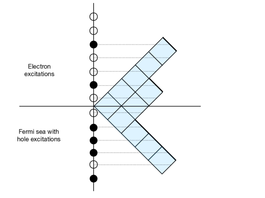
Figure 1: Each partition is associated with a state in the free-fermion Hilbert space. Here the partition $(5,3,1,1,1)$ (rotated by $45^{\circ}$) is associated with $\psi_{-\frac{3}{2}}\,\psi_{-\frac{9}{2}}\,\overline{\psi}_{-\frac{1}{2}}\,\overline{\psi}_{-\frac{9}{2}}\,\mid\!0\,\rangle$

The auxiliary matrix model and the determinantal expansion

We are now ready to translate our problem to the language of free fermions. For any ${\bf t}=(t_{1},t_{2},\dots)$ as in Section 24, we define the following state in the fermionic Fock space,

$$\mid\!{\bf t}\,\rangle\;\coloneqq\;\sum_{\boldsymbol{\mu}}S_{\boldsymbol{\mu}}({\bf t})\mid\!{\boldsymbol{\mu}}\,\rangle\,,$$ (44)

where $S_{\boldsymbol{\mu}}$ is the Schur function defined in (26), and the sum runs over all partitions as in the previous sections. The inner product between two such states is

$$\langle\,{\bf t}^{+}\!\mid\!{\bf t}^{-}\,\rangle\;=\;\sum_{\boldsymbol{\mu}}S_{\boldsymbol{\mu}}({\bf t}^{+})\,S_{\boldsymbol{\mu}}({\bf t}^{-})\;=\;\widetilde{Z}_{\infty}({\bf t}^{+},{\bf t}^{-})\,,$$ (45)

which is precisely the infinite-$N$ partition function (28) of the auxiliary model.

Now we come to finite $N$. Firstly, we note that inserting the occupation-number operator (39) at level $r$ between the two states introduces restrictions on the sum over partitions as follows,

$$\langle\,{\bf t}^{+}\!\mid N_{r}\mid\!{\bf t}^{-}\,\rangle\;=\;\sum_{r\,\in\,\mid\,\boldsymbol{\mu}\rangle}S_{\boldsymbol{\mu}}({\bf t}^{+})\,S_{\boldsymbol{\mu}}({\bf t}^{-})\quad\Leftrightarrow\quad\langle\,{\bf t}^{+}\!\mid(1-N_{r})\mid\!{\bf t}^{-}\,\rangle\;=\;\sum_{r\,\notin\,\mid\,\boldsymbol{\mu}\rangle}S_{\boldsymbol{\mu}}({\bf t}^{+})\,S_{\boldsymbol{\mu}}({\bf t}^{-})\,.$$ (46)

The restriction $\ell(\mu)\leq N$ in the sum (28) translates to $b_{s}<N$ in the Frobenius coordinates, which is to say that we sum over all partitions that do not contain any excitations around the vacuum of depth greater than $N$ inside the Fermi sea (Figure 2). From (46), we have

$$\widetilde{Z}_{N}({\bf t}^{+},{\bf t}^{-})\;=\;\sum_{\ell(\boldsymbol{\mu})\leq N}S_{\boldsymbol{\mu}}({\bf t}^{+})\,S_{\boldsymbol{\mu}}({\bf t}^{-})\;=\;\langle\,{\bf t}^{+}\!\mid\prod_{r<-N}(1-N_{r})\mid\!{\bf t}^{-}\,\rangle\,.$$ (47)

Upon expanding the infinite product, and using the expression for the number operator (39), we obtain

$$\widetilde{Z}_{N}({\bf t}^{+},{\bf t}^{-})\;=\;\sum_{m=0}^{\infty}(-1)^{m}\sum_{N<r_{1}<\dots<r_{m}}\!\!\langle\,{\bf t}^{+}\!\mid\psi_{r_{1}}\overline{\psi}_{-r_{1}}\dots\psi_{r_{m}}\overline{\psi}_{-r_{m}}\mid\!{\bf t}^{-}\,\rangle\,.$$ (48)

Figure 2: There is no hole in the bottom of the sea. For finite $N$, we can excite any number of holes at depths less than $N$ in the Fermi sea and can excite the same number of electrons at arbitrary heights above the sea. Some allowed configurations are shown for $N=3$.

It now remains to calculate the $2m$-point correlation functions in the expansion (48). Let’s first recall a much simpler problem, namely the evaluation of the same expectation values in the Dirac vacuum state. This is an elementary exercise involving moving all the positive energy modes to the right using the commutation relations (34) as summarized by Wick’s theorem, and it leads to the $m\times m$ determinant of 2-point functions, which can be evaluated in free field theory. Thus, the only non-trivial feature here is the dependence on the states $\mid\!{\bf t}^{\pm}\,\rangle$. As it turns out, this can be reduced to a free field calculation using another piece of the formalism—also very familiar to physicists—namely the bosonization of the two-dimensional complex chiral fermion. We review and summarize the main steps in Appendix B, and present the final answer for $\widetilde{Z}_{N}$ which is written as sum over determinants.

Theorem 4.1.

BO (00) (Determinantal formula for $\widetilde{Z}_{N}$)
With the notations as above, we have

$$\frac{\widetilde{Z}_{N}({\bf t}^{+},{\bf t}^{-})}{\widetilde{Z}_{\infty}({\bf t}^{+},{\bf t}^{-})}\;=\;\sum_{m=0}^{\infty}\,(-1)^{m}\,\!\!\sum_{N<r_{1}<\dots<r_{m}\atop r_{i}\in\mathbb{Z}+\tfrac{1}{2}}\det\bigl{(}\widetilde{K}(r_{i},r_{j}\,;\,{\bf t}^{+},{\bf t}^{-})\bigr{)}_{i,j=1}^{m}\,,$$ (49)

where $K(r_{i},r_{j}\,;\,{\bf t}^{+},{\bf t}^{-})$, $r_{i}\in\mathbb{Z}+\tfrac{1}{2}$ are given by the generating function

$$\widetilde{\kappa}(z,w;\,{\bf t}^{+},{\bf t}^{-})\;=\;\sum_{r,s\,\in\,\mathbb{Z}+\tfrac{1}{2}}\widetilde{K}(r,s\,;\,{\bf t}^{+},{\bf t}^{-})\,z^{r}\,w^{-s}\;=\;\frac{J(z;\,{\bf t}^{+},{\bf t}^{-})}{J(w;\,{\bf t}^{+},{\bf t}^{-})}\;\frac{\sqrt{zw}}{z-w}\,,\qquad|w|<|z|\,,$$ (50)

where

$$J(z;\,{\bf t}^{+},{\bf t}^{-})\;=\;\exp\biggl{(}\,\sum_{k=1}^{\infty}\,\frac{1}{k}\,t^{+}_{k}\,z^{k}-\sum_{k=1}^{\infty}\,\frac{1}{k}\,t^{-}_{k}\,z^{-k}\biggr{)}\,.$$ (51)

The expressions (50), (51) make it clear that $\widetilde{K}(r,s\,;\,{\bf t}^{+},{\bf t}^{-})$, which is the 2-point function in the fermionic theory, has minimal degree at least $r+s$ in the variables ${\bf t}^{+},{\bf t}^{-}$ and, therefore, the $m^{\text{th}}$ terms in (49) have minimal degree at least $2mN+m(m+1)$. Since $\widetilde{Z}_{\infty}$ has only non-negative powers of $t_{k}^{\pm}$, $k>0$, the previous statement about the minimal degree of the $m^{\text{th}}$ term also holds for $\widetilde{Z}_{N}({\bf t}^{+},{\bf t}^{-})$. Consequently, the coefficient of any given monomial in the variables $(t^{\pm}_{1},t^{\pm}_{2},\dots)$ in the left-hand side receives contributions only from a finite number of terms on the right-hand side and therefore is well-defined.

5 The giant graviton expansion

In this section we return to the original problem posed by the integral $Z_{N}({\bf g})$ defined in (1) and the specialization (3). Let us first take stock. We saw in Section 3 that $Z_{N}({\bf g})$ is related to the auxiliary integral $\widetilde{Z}_{N}({\bf t}^{+},{\bf t}^{-})$ defined in (18) as

$$Z_{N}({\bf g})\;=\;\left\langle{\,\widetilde{Z}_{N}\,}\right\rangle_{\bf g}\,,$$ (52)

where we recall the averaging operator $\left\langle{\,\cdot\,}\right\rangle_{\bf g}$ acts on power series $f({\bf t}^{+},{\bf t}^{-})$ as

$$\left\langle{\,f\,}\right\rangle_{\bf g}\;=\;\prod_{k=1}^{\infty}\int\frac{\mathrm{d}t_{k}^{+}\,\mathrm{d}t_{k}^{-}}{2\pi kg_{k}}\,{\rm e}^{-t_{k}^{+}\,t_{k}^{-}/kg_{k}}\,f({\bf t}^{+},{\bf t}^{-})\,.$$ (53)

At $N=\infty$, the two integrals reduce to

$$Z_{\infty}({\bf g})\;=\;\prod_{k=1}^{\infty}\frac{1}{1-g_{k}}\,,\qquad\widetilde{Z}_{\infty}({\bf t}^{+},{\bf t}^{-})\;=\;\exp\biggl{(}\,\sum_{k=1}^{\infty}\frac{1}{k}\,t^{+}_{k}\,t^{-}_{k}\biggr{)}\,,$$ (54)

for which the relation (52) can be easily verified.

For finite $N$ we have the formula (49) for the auxiliary matrix integral, in terms of the 2-point function $\widetilde{K}(r,s\,;\,{\bf t}^{+},{\bf t}^{-})$ given by (50). Now we need to calculate the average (52). Note that, if we have $t_{k}^{\pm}$ to be complex conjugate variables, and if the states $\mid\!{\bf t}^{-}\,\rangle$ span a complete basis of states, then the required average is the expectation value

$$Z_{N}({\bf g})\;=\;\mbox{Tr}\,\Bigl{(}\,\textstyle{\prod_{r<-N}(1-N_{r})}\,\rho_{\bf g}\Bigr{)}$$ (55)

of the operator in the right-hand side of Equation (47) in the quantum statistical state defined by the density operator

$$\rho_{\bf g}\;=\;\exp(-{\bf t^{+}}{\bf t^{-}}/{\bf g})\mid\!{\bf t^{-}}\,\rangle\langle\,\bf t^{+}\!\mid\,,$$ (56)

with the trace and the exponential defined by the conventions in (53).

It is convenient to define a normalized transformation acting on each term in (49) as follows,

$$K^{(m)}_{\bf g}(r_{1},\dots,r_{m})\;\coloneqq\;\frac{1}{Z_{\infty}({\bf g})}\left\langle{\,\widetilde{Z}_{\infty}\,\det\bigl{(}\widetilde{K}(r_{i},r_{j})\bigr{)}_{i,j=1}^{m}\,}\right\rangle_{\bf g}\,.$$ (57)

We reach the formula for $Z_{N}({\bf g})$ by summing (57) over all $m$-tuples of points in $\mathbb{Z}+\tfrac{1}{2}$ as in (49), and then summing over $m=1,2,\dots$. We have already seen that the $m^{\text{th}}$ term in the expansion for $\widetilde{Z}_{N}({\bf t}^{+},{\bf t}^{-})$ has minimal degree in $({\bf t}^{+},{\bf t}^{-})$ at least $2mN+m(m+1)$. From the action (22) of the H-S transformation on monomials, and the fact that $Z_{\infty}({\bf g})$ has only non-negative powers of $g_{k}$, we see that the $m^{\text{th}}$ term in the expansion for $Z_{N}({\bf t}^{+},{\bf t}^{-})$ has minimal degree in ${\bf g}$ at least $mN+m(m+1)/2$, and therefore the sum over $m$ is convergent in the power-series sense. We have proved the following proposition.

Proposition 5.1.

(A systematic expansion for $Z_{N}$)
The unitary matrix integral

$$Z_{N}({\bf g})\;=\;\int_{U(N)}\,\mathrm{d}U\,\exp\biggl{(}\;\sum_{k=1}^{\infty}\,\frac{1}{k}\,g_{k}\,\mbox{Tr}\,U^{k}\,\mbox{Tr}\,U^{-k}\,\biggr{)}\,,$$ (58)

is given by the expansion

$$\frac{Z_{N}({\bf g})}{Z_{\infty}({\bf g})}\;=\;\sum_{m=0}^{\infty}\,G^{(m)}_{N}({\bf g})\,,$$ (59)

with $G^{(0)}_{N}({\bf g})=1$ and

$$G^{(m)}_{N}({\bf g})\;=\;(-1)^{m}\sum_{N<r_{1}<\dots<r_{m}\atop r_{i}\in\mathbb{Z}+\tfrac{1}{2}}K^{(m)}_{\bf g}(r_{1},\dots,r_{m})\,,\qquad m\;=\;1,2,\dots\,,$$ (60)

where the functions $K^{(m)}_{\bf g}$ are given in Equation (57). The minimal degree of the series $G^{(m)}_{N}({\bf g})$ is not less than $mN+m(m+1)/2$.

We call the $G^{(m)}_{N}$ the contribution from $m$ giant gravitons for reasons explained in the introduction. The above proposition gives a well-defined expansion for $Z_{N}({\bf g})$ with each term being the Hubbard-Stratonovich transformation of a determinant of two-point functions in our auxiliary theory. Performing the integrals involved in the transformation leads to further simplification. We now demonstrate this for the first non-trivial term in the expansion (59), namely the contribution of one giant graviton.

The contribution of one giant graviton is given in terms of the H-S transformation of the two-point function $\widetilde{K}(r,s;\,{\bf t}^{+},{\bf t}^{-})$,

$$\left\langle{\,\widetilde{Z}_{\infty}\,\widetilde{K}(r,s)\,}\right\rangle_{\bf g}\,\quad\text{with~{}$r=s$}.$$ (61)

We consider the generating function of (61), with one variable which tracks the power of $r(=s)$. Recalling from (22) that the H-S transform vanishes when the power of ${\bf t}^{+}$ and ${\bf t}^{-}$ are not equal, we see that one can sum over all values of $(r,s)$ with two corresponding variables, and the resulting function should only depend on one combination of the two variables. With this in mind, we consider

$$\begin{split}&\sum_{r,s\in\mathbb{Z}+\tfrac{1}{2}}z^{r}\,w^{-s}\,\left\langle{\,\widetilde{Z}_{\infty}\,\widetilde{K}(r,s)\,}\right\rangle_{\bf g}\ \;=\;\left\langle{\,\widetilde{Z}_{\infty}\;\widetilde{\kappa}(z,w)\,}\right\rangle_{\bf g}\\ &\qquad\;=\;\frac{\sqrt{zw}}{z-w}\,\prod_{k=1}^{\infty}\int\frac{\mathrm{d}t_{k}^{+}\,\mathrm{d}t_{k}^{-}}{2\pi kg_{k}}\,\exp\biggl{(}\frac{1}{k}\Bigl{(}-\frac{t_{k}^{+}\,t_{k}^{-}}{g_{k}}+t_{k}^{+}\,t_{k}^{-}+t_{k}^{+}(z^{k}-w^{k})-t_{k}^{-}(z^{-k}-w^{-k})\Bigr{)}\biggr{)}\,,\end{split}$$ (62)

where we have interchanged the order of sum and averaging operations, and used (50). Using the Gaussian integral formula (21) we obtain, for $|w/z|<1$,

$$\begin{split}&\sum_{r,s\in\mathbb{Z}+\tfrac{1}{2}}z^{r}\,w^{-s}\,\left\langle{\,\widetilde{Z}_{\infty}\,\widetilde{K}(r,s)\,}\right\rangle_{\bf g}\\ &\qquad\qquad\;=\;Z_{\infty}({\bf g})\,\frac{\sqrt{w/z}}{1-w/z}\,\exp\biggl{(}\,\sum_{k=1}^{\infty}\frac{1}{k}\,\gamma_{k}\,\Bigl{(}-2+\Bigl{(}\frac{w}{z}\Bigr{)}^{k}+\Bigl{(}\frac{w}{z}\Bigr{)}^{-k}\Bigr{)}\biggr{)}\,,\qquad\qquad\end{split}$$ (63)

where we have defined a new set of coupling constants,

$$\gamma_{k}\;\coloneqq\;\frac{g_{k}}{1-g_{k}}\,.$$ (64)

As anticipated above, the final expression for the transformed generating function (63) is diagonal. After dividing through by $Z_{\infty}({\bf g})$, we obtain the generating function for $K^{(1)}_{\bf g}(r)$,

$$\sum_{r\in\mathbb{Z}+\tfrac{1}{2}}\zeta^{-r}\,K^{(1)}_{\bf g}(r)\;=\;\frac{\sqrt{\zeta}}{1-\zeta}\,\exp\biggl{(}\,\sum_{k=1}^{\infty}\frac{1}{k}\,\gamma_{k}\,\bigl{(}-2+\zeta^{k}+\zeta^{-k}\bigr{)}\biggr{)}\,.$$ (65)

We now see that the sum that we need in (60),

$$G^{(1)}_{N}({\bf g})\;=\;-\sum_{N<r}K^{(1)}_{\bf g}(r)\,,$$ (66)

is equal to the negative of the $\zeta^{-N}$ coefficient of the left-hand side of (65) multiplied by $\sqrt{\zeta}/(1-\zeta)$. Multiplying the right-hand side with the same factor thus gives us the corresponding generating function. We have thus proved the following proposition.

Proposition 5.2.

(Contribution of one giant)
The generating series

$$\widehat{K}(\zeta;\bm{\gamma})\;=\;-\sum_{N\in\mathbb{Z}}\,\zeta^{-N}\,G^{(1)}_{N}({\bf g})\,,$$ (67)

for the contribution $G^{(1)}_{N}({\bf g})$ of one giant-graviton to the expansion (59), equals

$$\widehat{K}(\zeta;\bm{\gamma})\;=\;\frac{\zeta}{(1-\zeta)^{2}}\,\exp\biggl{(}\,\sum_{k=1}^{\infty}\frac{1}{k}\,\gamma_{k}\,\bigl{(}-2+\zeta^{k}+\zeta^{-k}\bigr{)}\biggr{)}\,,$$ (68)

where $\bm{\gamma}=(\gamma_{1},\gamma_{2},\dots)$ is given by $\gamma_{k}=g_{k}/(1-g_{k})$, $k=1,2,\dots$.

Specialization to $g_{k}=f(q^{k})$

The index (3) is now easily evaluated by specializing the above considerations to couplings given in terms of a power series $g_{k}=f(q^{k})$. Proposition 5.1 leads to a convergent expansion for a power series in $q$, and Proposition 5.2 naturally leads to a new set of couplings and power series,

$$\gamma_{k}\;=\;\widehat{f}(q^{k})\,,\qquad\widehat{f}(q)\;=\;\frac{f(q)}{1-f(q)}\,,$$ (69)

and the generating function

$$\widehat{K}_{f}(\zeta,q)\;=\;\widehat{K}\bigl{(}\zeta;(\widehat{f}(q),\widehat{f}(q^{2}),\dots)\bigr{)}\,.$$ (70)

We summarize our findings in terms of the following theorems.

Theorem 5.1.

(Giant graviton expansion for the index)
For any power series $f(q)=\sum_{k=1}^{\infty}a_{k}\,q^{k}$ of order $\alpha$, the matrix integral

$$I^{f}_{N}(q)\;=\;\int_{U(N)}\,\mathrm{d}U\,\exp\biggl{(}\;\sum_{k=1}^{\infty}\,\frac{1}{k}\,f(q^{k})\,\mbox{Tr}\,U^{k}\,\mbox{Tr}\,U^{-k}\,\biggr{)}$$ (71)

admits a $q$-expansion

$$\frac{I^{f}_{N}(q)}{I^{f}_{\infty}(q)}\;=\;\sum_{m=0}^{\infty}\,G^{(m)}_{f,N}(q)\,,\qquad I^{f}_{\infty}(q)=\prod_{k=1}^{\infty}\frac{1}{1-f(q^{k})}\,,$$ (72)

where $G^{(m)}_{f,N}(q)$, $m=0,1,2,\dots$ is given by the formula (60) with ${\bf g}=(f(q),f(q^{2}),\dots)$, and has order at least $\alpha mN+\alpha m(m+1)/2$ as a power series in $q$.

Theorem 5.2.

(The contribution of one giant)
With the set up of Theorem 5.1, we have that $G^{(1)}_{f,N}(q)$ is the coefficient of $\zeta^{-N}$ in the expansion of

$$\widehat{K}_{f}(\zeta,q)\;=\;\frac{1}{(1-\zeta)\,(1-1/\zeta)}\,\prod_{n=1}^{\infty}\,\biggl{(}\frac{(1-q^{n})^{2}}{(1-q^{n}\,\zeta)\,(1-q^{n}/\zeta)}\biggr{)}^{\widehat{a}_{n}}\,,$$ (73)

in the range $|q|<|\zeta|<1$, where the integers $\widehat{a}_{n}$ are summarized by their generating function $\widehat{f}(q)=\sum_{n=1}^{\infty}\,\widehat{a}_{n}\,q^{n}$ given by

$$\widehat{f}(q)\;=\;\frac{f(q)}{1-f(q)}\,.$$ (74)

Comments and implications

1. The expansion of the infinite product (73) should be performed first in $q$, as consistent with the range. The coefficient of $q^{m}$ is seen to be a polynomial in $\zeta,1/\zeta$ of order $m$. We can then reinterpret the expansion as a Laurent series in $\zeta$, where the coefficient of $\zeta^{n}$ is a $q$-series (which has order at least $|n|$).

2. The bound given on the order of $G^{(m)}_{f,N}(q)$ is not strict. For $m=1$ the order is indeed $\alpha(N+1)$, but the bound can be improved in general. Recall that the bound was derived by calculating the smallest power in ${\bf t}^{+},{\bf t}^{-}$ in the elements of the matrix $\bigl{(}\widetilde{K}(r_{i},r_{j}\,;\,{\bf t}^{+},{\bf t}^{-})\bigr{)}_{i,j=1}^{m}$ and then translating the consequent bound on the determinant to powers of $q$ after the integral transform. The point is that there can be cancellations in the determinants for $m\geq 2$. Indeed, the lowest term in the above process is the determinant of the matrix $\bigl{(}q^{\alpha\,N+\alpha(i+j)/2}\bigr{)}_{i,j=1}^{m}$, which vanishes. The order of $G^{(m)}_{f,N}(q)$ is, therefore, at least $\alpha(mN+m(m+1)/2+1)$ for $m\geq 2$.

3. It is clear from the above considerations that the contributions of multiple giants will be Taylor coefficients of certain infinite products whose multiplicities are determined by $f(q)$, in a manner similar to Theorem 5.2.

4. The formula (72) is an exact formula which means that the full index is captured by bound states of giant-gravitons and gravitons. This is quite surprising from the AdS/CFT viewpoint, and is reminiscent of similar phenomena in AdS₃ space Ebe (21).

5. The gauge theory index $I^{f}_{N}(q)$ at finite $N$ can be interpreted holographically as follows. Say $f(q)=a_{1}q+a_{2}q^{2}+\dots$, $a_{1}\neq 0$. Then the first $N$ coefficients are given by the multi-graviton formula $I^{f}_{\infty}$, the next $N$ coefficients are given by the contribution of one giant graviton (with multi-graviton fluctuations on top), and so on.

6. The formula (73) is similar to the formula for the superconformal index with the power series $\widehat{f}(q)$ playing the role of the single-particle index. It should be interpreted as the single-particle index of the giant gravitons, following the ideas in AI (19); Ima (21); GL (21). The map $f\mapsto\widehat{f}$ should be accounted for by the curvature of the D-branes in AdS space, but it would be nice to understand this in detail.

7. The structure of the expansion in Theorems 5.1, 5.2 points to a duality which interchanges $m\leftrightarrow N$. This duality should be regarded as a manifestation of the open-closed-open duality of Gop (10) in the BPS sector of the theory.

8. The final formula (72) expresses a microscopic quantity—the gauge theory partition function—as an ensemble average in a free fermionic theory or, equivalently, an average over matrix model theories. It may serve as a good example to test ideas in the physics literature relating such averages to black holes MS (16).

6 Examples

The statements in the theorems 5.1, 5.2 hold for an arbitrary power series $f(q)$ of the type considered therein, and it is illuminating to check it numerically for a given power series of interest. In this section we illustrate the consequences of the theorems for the BPS indices of the $\mathcal{N}=4$ super Yang-Mills theory given in (4).

We use the following notation for the Pochhamer symbols,

$$(q)_{n}\;=\;\prod_{k=1}^{n}\,(1-q^{k})\,,\quad(q)_{\infty}\;=\;\prod_{k=1}^{\infty}\,(1-q^{k})\,,\quad(x;q)_{\infty}\;=\;\prod_{k=0}^{\infty}(1-xq^{k})\,.$$ (75)

$\tfrac{1}{2}$-BPS index

Here we specialize to $f(q)=f_{1/2}(q)=q$. It is well-known that $I^{1/2}_{N}(q)=1/(q)_{N}$, and this was also presented as a motivating example in GL (21). We quickly work through the formula from the perspective of random partitions that we take here. The formula (14) gives

$$I^{1/2}_{N}(q)\;=\;\sum_{\boldsymbol{\lambda}}\,q^{|\boldsymbol{\lambda}|}\,\frac{1}{z_{\boldsymbol{\lambda}}}\,\sum_{\ell(\boldsymbol{\mu})\leq N}\,\chi^{\boldsymbol{\mu}}(\boldsymbol{\lambda})^{2}\,.$$ (76)

We now perform the sum over $\boldsymbol{\lambda}$ for a fixed weight $|\boldsymbol{\lambda}|=n$ and a fixed length $\ell(\boldsymbol{\mu})=k$ to obtain

$$\sum_{|\boldsymbol{\lambda}|=n}\frac{1}{z_{\boldsymbol{\lambda}}}\,\sum_{\ell(\boldsymbol{\mu})=k}\,\chi^{\boldsymbol{\mu}}(\boldsymbol{\lambda})^{2}\;=\;P(n,k)\,,$$ (77)

where $P(n,k)$ is the partition of $n$ into $k$ parts. This leads to

$$I^{1/2}_{N}(q)\;=\;\sum_{n=0}^{\infty}\sum_{k=0}^{N}\,P(n,k)\,q^{n}\;=\;\frac{1}{(q)_{N}}\,,$$ (78)

which is a well-known formula.

In this case the giant graviton expansion can be fully understood. Firstly, we have

$$I^{1/2}_{\infty}(q)\;=\;\frac{1}{(q)_{\infty}}\,,$$ (79)

which is indeed the multi-graviton index. Then we have

$$\frac{I^{1/2}_{N}(q)}{I^{1/2}_{\infty}(q)}\;=\;\frac{(q)_{\infty}}{(q)_{N}}\;=\;(q^{N+1};q)_{\infty}\,.$$ (80)

We use the identity (see e.g. Zag (07) Chapter 2, Proposition 2)

$$(x;q)_{\infty}\;=\;\sum_{m=0}^{\infty}\,\frac{(-1)^{m}\,q^{m\choose 2}}{(q)_{m}}\,x^{m}$$ (81)

to obtain the complete giant-graviton expansion

$$\frac{I^{1/2}_{N}(q)}{I^{1/2}_{\infty}(q)}\;=\;\sum_{m=0}^{\infty}\,\frac{(-1)^{m}\,q^{m+1\choose 2}}{(q)_{m}}\,q^{mN}\,.$$ (82)

Now let us check our formula. We have

$$\widehat{f}_{1/2}(q)\;=\;\frac{q}{1-q}\;=\;\sum_{n=1}^{\infty}\,q^{n}\,,\qquad\widehat{K}_{\frac{1}{2}}(\zeta,q)\;=\;\frac{(q;q)_{\infty}^{2}}{(\zeta;q)_{\infty}\,(1/\zeta;q)_{\infty}}\,.$$ (83)

We expand $\widehat{K}$ in powers of $q$ and then $\zeta$, as explained above, to obtain the giant-graviton contributions

$$\widehat{K}_{\frac{1}{2}}(\zeta,q)\;=\;\sum_{N\in\mathbb{Z}}\,\zeta^{-N}\,\widehat{G}^{(1)}_{\frac{1}{2},N}(q)\,,\qquad|q|<|\zeta|<1\,.$$ (84)

We find:
$N=1$

$$\begin{split}G^{(1)}_{\frac{1}{2},1}(q)&\;=\;-q^{2}-q^{3}-q^{4}\,{\color[rgb]{0,0,1}-\;q^{6}-q^{8}-q^{9}-q^{10}-2q^{12}-q^{15}+\dots}\,,\\ \frac{I^{1/2}_{1}(q)}{I^{1/2}_{\infty}(q)}-1&\;=\;-q^{2}-q^{3}-q^{4}\,{\color[rgb]{0,0,1}+\;q^{7}+q^{8}+q^{9}+q^{10}+q^{11}-q^{15}+\dots}\,.\\ \end{split}$$ (85)

$N=2$

$$\begin{split}G^{(1)}_{\frac{1}{2},2}(q)&\;=\;-q^{3}-q^{4}-q^{5}-q^{6}\,{\color[rgb]{0,0,1}-\;q^{8}-q^{10}-2q^{12}-q^{14}+\dots}\,,\\ \frac{I^{1/2}_{2}(q)}{I^{1/2}_{\infty}(q)}-1&\;=\;-q^{3}-q^{4}-q^{5}-q^{6}\,{\color[rgb]{0,0,1}+\;q^{9}+q^{10}+2q^{11}+q^{12}+2q^{13}+q^{14}+\dots}\,.\end{split}$$ (86)

$N=3$

$$\begin{split}G^{(1)}_{\frac{1}{2},3}(q)&\;=\;-q^{4}-q^{5}-q^{6}-q^{7}-q^{8}\,{\color[rgb]{0,0,1}-\,q^{10}-q^{12}-q^{14}-q^{15}-q^{16}+\dots}\,,\\ \frac{I^{1/2}_{3}(q)}{I^{1/2}_{\infty}(q)}-1&\;=\;-q^{4}-q^{5}-q^{6}-q^{7}-q^{8}\,{\color[rgb]{0,0,1}+\;q^{11}+q^{12}+2q^{13}+2q^{14}+2q^{15}+2q^{16}+\dots}\,.\end{split}$$ (87)

We see that $G^{(1)}_{\frac{1}{2},N}(q)$ has order $N+1$, and agrees with the expansion (82) (recall that $G^{(0)}_{\frac{1}{2},N}=1$), up to $\text{O}(q^{2N+4})$ as predicted.

$\frac{1}{8}$-BPS index

Here we have $f(q)=2q/(1+q)$, for which the superconformal index is called the Schur index GRRY (13). This index has been studied in quite some depth, including from the point of view of modular transformations Raz (12); BRS (21); PP (21). The following explicit expression for the Schur index was obtained in BDF (15),

$$I^{1/8}_{N}(q)\;=\;\frac{1}{(q;q)_{\infty}\,(q;q^{2})_{\infty}}\,\sum_{m=0}^{\infty}\,(-1)^{m}\,\biggl{(}\binom{N+m}{N}+{N+m-1\choose N}\biggr{)}\,q^{mN+m^{2}}\,.$$ (88)

Firstly, we note that the prefactor in (88) is indeed equal to

$$\frac{1}{(q;q)_{\infty}\,(q;q^{2})_{\infty}}\;=\;\prod_{n=1}^{\infty}\,\frac{1+q^{n}}{1-q^{n}}\;=\;I_{\infty}^{1/8}(q)\,,$$ (89)

where the last equality follows from the formula (15) with $f^{1/8}(q)=2q/(1+q)$. Thus we have

$$\frac{I^{1/8}_{N}(q)}{I^{1/8}_{\infty}(q)}\;=\;\sum_{m=0}^{\infty}\,(-1)^{m}\,\biggl{(}\binom{N+m}{N}+{N+m-1\choose N}\biggr{)}\,q^{mN+m^{2}}\,,$$ (90)

which is in the form of the giant graviton expansion.

Now let us check our formula. We have

$$\widehat{f}_{1/8}(q)\;=\;\frac{2q}{1-q}\;=\;\;=\;2\sum_{n=1}^{\infty}\,q^{n}\,,\qquad\widehat{K}_{\frac{1}{8}}(\zeta,q)\;=\;\frac{1}{(1-\zeta)(1-1/\zeta)}\frac{(q;q)_{\infty}^{4}}{(\zeta q;q)_{\infty}^{2}\,(q/\zeta;q)_{\infty}^{2}}\,.$$ (91)

We find, upon expanding $\widehat{K}_{\frac{1}{8}}$, the contributions of $N=1,2,3$:

$$\begin{split}G^{(1)}_{\frac{1}{8},1}(q)&\;=\;-3q^{2}-5q^{6}-7q^{12}-9q^{20}+\text{O}(q^{21})\,,\\ G^{(1)}_{\frac{1}{8},2}(q)&\;=\;-4q^{3}-6q^{8}-8q^{15}+\text{O}(q^{21})\,,\\ G^{(1)}_{\frac{1}{8},3}(q)&\;=\;-5q^{4}-7q^{10}-9q^{18}+\text{O}(q^{21})\,.\end{split}$$ (92)

We can check that $G^{(1)}_{N}(q)$ has order $N+1$ and agrees with the expansion (90) up to $\text{O}(q^{2N+4})$ as predicted.

$\frac{1}{16}$-BPS index

Here we have

$$\begin{split}f_{1/16}(q)&\;=\;1-\frac{(1-q^{2})^{3}}{(1-q^{3})^{2}}\;=\;\frac{q^{2}(3+4q+2q^{2})}{(1+q+q^{2})^{2}}\,,\\ &\;=\;3\sum_{n=1}^{\infty}\,n\,q^{3n-1}-2\sum_{n=1}^{\infty}\,q^{3n}-3\sum_{n=1}^{\infty}\,n\,q^{3n+1}\,,\qquad\qquad\qquad\end{split}$$ (93)

$$\begin{split}\widehat{f}_{1/16}(q)&\;=\;\frac{(1-q^{3})^{2}}{(1-q^{2})^{3}}-1\;=\;\frac{q^{2}(3+4q+2q^{2})}{(1-q)(1+q)^{3}}\,,\\ &\;=\;\sum_{n=1}^{\infty}\,(n^{2}+2)\,q^{2n}-\sum_{n=1}^{\infty}\,n(n-1)\,q^{2n-1}\,.\qquad\qquad\qquad\qquad\end{split}$$ (94)

In this case no explicit formula (e.g. of the type (88)) is known which does not involve the evaluation of multi-dimensional contour integrals (1) or the evaluation of symmetric group characters (14). Using the latter method the index up to $\text{O}(q^{70})$ was calculated in Mur (22). Here $f_{1/16}(q)=\text{O}(q^{2})$, so that $\alpha=2$ in the notation of Theorem 5.1. This means that $G^{(1)}_{{\frac{1}{16},N}}(q)=\text{O}(q^{2(N+1)})$, and so the non-trivial check with the first 70 terms can be made for up to $N=34$. We have verified the statement of our theorem that $G^{(1)}_{{\frac{1}{16},N}}(q)$ agrees with the expansion (90) up to $\text{O}(q^{4N+8})$ up to this rank. We present the first three cases below. We note that the functions $\widehat{K}_{\frac{1}{16}}(\zeta,q)$ are infinite products of terms of the type $(1-q^{n})^{n}$ and $(1-q^{n})^{n^{2}}$, generalizing the MacMahon function, such functions are being studied in work in progress by the author with S. Garoufalidis and D. Zagier.

$N=1$

$$\begin{split}G^{(1)}_{\frac{1}{16},1}(q)&\;=\;-6q^{4}+6q^{5}-3q^{6}-6q^{7}+21q^{8}-36q^{9}+27q^{10}+30q^{11}{\color[rgb]{0,0,1}-148q^{12}+270q^{13}}\\ &\qquad{\color[rgb]{0,0,1}-336q^{14}+202q^{15}+348q^{16}-1392q^{17}+\dots}\,,\\ \frac{I^{1/16}_{1}(q)}{I^{1/16}_{\infty}(q)}-1&\;=\;-6q^{4}+6q^{5}-3q^{6}-6q^{7}+21q^{8}-36q^{9}+27q^{10}+30q^{11}{\color[rgb]{0,0,1}-92q^{12}+132q^{13}}\\ &\qquad{\color[rgb]{0,0,1}-90q^{14}-106q^{15}+369q^{16}-444q^{17}+\dots}\,.\\ \end{split}$$ (95)

$N=2$

$$\begin{split}G^{(1)}_{\frac{1}{16},2}(q)&\;=\;-10q^{6}+12q^{7}-9q^{8}+21q^{10}-54q^{11}+83q^{12}-102q^{13}+72q^{14}+128q^{15}\\ &\qquad{\color[rgb]{0,0,1}-585q^{16}+1122q^{17}+\dots}\,,\\ \frac{I^{1/16}_{2}(q)}{I^{1/16}_{\infty}(q)}-1&\;=\;-10q^{6}+12q^{7}-9q^{8}+21q^{10}-54q^{11}+83q^{12}-102q^{13}+72q^{14}+128q^{15}\\ &\qquad{\color[rgb]{0,0,1}-459q^{16}+744q^{17}+\dots}\,.\end{split}$$ (96)

$N=3$

$$\begin{split}G^{(1)}_{\frac{1}{16},3}(q)&\;=\;-15q^{8}+20q^{9}-18q^{10}+12q^{11}+10q^{12}-54q^{13}+111q^{14}-190q^{15}+279q^{16}\\ &\qquad-288q^{17}+49q^{18}+630q^{19}{\color[rgb]{0,0,1}-1905q^{20}+3658q^{21}+\dots}\,,\\ \frac{I^{1/16}_{2}(q)}{I^{1/16}_{\infty}(q)}-1&\;=\;-15q^{8}+20q^{9}-18q^{10}+12q^{11}+10q^{12}-54q^{13}+111q^{14}-190q^{15}+279q^{16}\\ &\qquad-288q^{17}+49q^{18}+630q^{19}{\color[rgb]{0,0,1}-1653q^{20}+2790q^{21}+\dots}\,.\end{split}$$ (97)

Appendix A The matrix integral as a sum over partitions

We use the notations and conventions of Macon . We denote partitions as $\boldsymbol{\lambda}=(\lambda_{1},\lambda_{2},\dots)$ with $\lambda_{1}\geq\lambda_{2}\geq\dots$, or in the frequency representation as $\prod_{i\geq 1}i^{\,r_{i}}=1^{r_{1}}\,2^{r_{2}}\,\dots$. The number of parts of a partition (or length) is the number of non-zero $\lambda_{i}$ or, equivalently, $\ell(\boldsymbol{\lambda})\;=\;\sum_{i}r_{i}$. The weight of the partition $|\boldsymbol{\lambda}|=\sum_{j\geq 1}\lambda_{j}\;=\;\sum_{i\geq 1}\,i\,r_{i}$. The first step is to expand the exponential in (1), which gives a sum of products of traces of powers of the unitary matrix and powers of its inverse. Each such product $\prod_{i\geq 1}\,\bigl{(}\mbox{Tr}\,U^{i}\bigr{)}^{r_{j}}$ is labelled by the partition $\boldsymbol{\lambda}=\prod_{i\geq 1}i^{\,r_{i}}$ written in the frequency representation, and we denote such a product by $\mathcal{O}_{\boldsymbol{\lambda}}(U)$ (and similarly we have $\mathcal{O}_{\boldsymbol{\lambda}}(U^{-1})$.) Next we write these powers in terms of $U(N)$ group characters FH (04). Recall that the representations of $U(N)$ and those of the symmetric group $S_{N}$ are both labelled by partitions of $N$. We denote the corresponding characters as $\widetilde{\chi}_{\boldsymbol{\mu}}$ and $\chi^{\boldsymbol{\mu}}$, respectively. We then use the Frobenius formula for $U(N)$,

$$\mathcal{O}_{\boldsymbol{\lambda}}(U)\;=\;\sum_{\ell(\boldsymbol{\mu})\leq N}\,\widetilde{\chi}_{\boldsymbol{\mu}}(U)\,\chi^{\boldsymbol{\mu}}(\boldsymbol{\lambda})\,.$$ (98)

Here, and below, all sums over partitions run over all partitions with any restrictions being indicated (as in the sum over $\boldsymbol{\mu}$).

Using the first orthogonality relation of the group characters of $U(N)$, i.e.,

$$\int\,DU\,\widetilde{\chi}_{\boldsymbol{\mu}}(U)\,\widetilde{\chi}_{\boldsymbol{\mu}^{\prime}}(U^{-1})\;=\;\delta_{\boldsymbol{\mu}\boldsymbol{\mu}^{\prime}}\,,$$ (99)

we obtain

$$\int\,DU\,\mathcal{O}_{\boldsymbol{\lambda}}(U)\,\mathcal{O}_{\boldsymbol{\lambda}}(U^{-1})\;=\;\sum_{\ell(\boldsymbol{\mu})\leq N}\,\chi^{\boldsymbol{\mu}}(\boldsymbol{\lambda})\;\overline{\chi^{\boldsymbol{\mu}}(\boldsymbol{\lambda})}\;=\;\sum_{\ell(\boldsymbol{\mu})\leq N}\,\chi^{\boldsymbol{\mu}}(\boldsymbol{\lambda})^{2}\,.$$ (100)

Here the second equality is a consequence of the fact that the characters of the symmetric group are real (actually integers). Upon putting these steps together, we obtain

$$\begin{split}Z_{N}({\bf g})&\;=\;\int\,DU\,\sum_{\boldsymbol{\lambda}}\frac{{\bf g}^{\boldsymbol{\lambda}}}{z_{\boldsymbol{\lambda}}}\;\mathcal{O}_{\boldsymbol{\lambda}}(U)\,\mathcal{O}_{\boldsymbol{\lambda}}(U^{\dagger})\\ &\;=\;\sum_{\boldsymbol{\lambda}}\,\frac{{\bf g}^{\boldsymbol{\lambda}}}{z_{\boldsymbol{\lambda}}}\,\sum_{\ell(\boldsymbol{\mu})\leq N}\,\chi^{\boldsymbol{\mu}}(\boldsymbol{\lambda})^{2}\,,\end{split}$$ (101)

where, for any partition $\boldsymbol{\lambda}$ as above, we use the notations

$${\bf g}^{\boldsymbol{\lambda}}\;\coloneqq\;\prod_{j\geq 1}\,g_{\lambda_{j}}\;=\;\prod_{i\geq 1}\,g_{i}^{r_{i}}\,,\qquad z_{\boldsymbol{\lambda}}\;\coloneqq\;\prod_{i}\,r_{i}!\,i^{r_{i}}\,.$$ (102)

Appendix B Review of bosonization and fermionic correlation functions

We first recall the basic ideas and equations of bosonization that we need here Gin (88) (we use the conventions of Pol (07)). We introduce a real chiral bosonic field $X(z)$ which obeys the operator product expansion

$$\partial X(z)\,\partial X(w)\;\sim\;-\frac{1}{(z-w)^{2}}+\text{O}(1)\,.$$ (103)

The field is expanded in oscillator modes as

$$\partial X(z)\;=\;-\mathrm{i}\,\sum_{n\in\mathbb{Z}}\frac{\alpha_{n}}{z^{n+1}}\,.$$ (104)

The oscillator modes obey ${\alpha}^{\dagger}_{n}=\alpha_{-n}$, and the OPE (103) is equivalent to the commutation relations

$$\bigl{[}\,\alpha_{n}\,,\,\alpha_{m}\,\bigr{]}\;=\;n\,\delta_{n+m,0}\,.$$ (105)

We call $\alpha_{n}$ bosonic creation operators for $n<0$ and annihilation operators for $n>0$. The bosonic vacuum is defined to be the state

$$\alpha_{n}\mid\!0\,\rangle\;=\;0\,,\qquad n>0\,.$$ (106)

States in the bosonic Fock space are spanned by an arbitrary number of creation operators acting on the vacuum state. The mode $\alpha_{0}$ corresponds to the momentum in field space and needs to be quantized separately. As it turns out, we do not need to deal with this zero mode for our purposes, and therefore we will only discuss the modes $n$ in $\mathbb{Z}^{*}=\mathbb{Z}\,\backslash\,\{0\}$ in the formulas below. We will also not discuss cocycles in any of the vertex operators, as we do not need them for our purposes.

The basic statement of bosonization is that the free complex chiral fermion discussed in Section 4 is equivalent to the free chiral boson with the relations

$$\psi(z)\;=\;:{\rm e}^{+\mathrm{i}\,X(z)}:\,,\qquad\overline{\psi}(z)\;=\;:{\rm e}^{-\mathrm{i}\,X(z)}:\,,$$ (107)

where the $:\cdot:$ indicates normal ordering. Equivalently, we can present the relation between the fermionic and the bosonic modes,

$$\alpha_{n}\;=\;\sum_{r\in\mathbb{Z}+\tfrac{1}{2}}\,\overline{\psi}_{n-r}\,\psi_{r}\,,\qquad n\in\mathbb{Z}^{*}\,.$$ (108)

The bosonic vacuum maps to the Dirac vacuum. We will also need the commutation relations of the bosonic oscillator modes with the fermions, which follow from (107),

$$\bigl{[}\,\alpha_{n}\,,\,\psi(z)\,\bigr{]}\;=\;z^{n}\,\psi(z)\,,\qquad\bigl{[}\,\alpha_{n}\,,\,\overline{\psi}(z)\,\bigr{]}\;=\;-z^{n}\,\overline{\psi}(z)\,,\qquad n\in\mathbb{Z}^{*}\,.$$ (109)

Next we write the state $\mid\!\bf t\,\rangle$ defined in (44) in terms of the bosonic variables. This needs some basics of symmetric function theory Macon . An important role in the following is played by the following vertex operators

$$\Gamma_{\pm}({\bf t})\;\coloneqq\;\exp\biggl{(}\,\sum_{k=1}^{\infty}\frac{1}{k}\,t_{k}\,\alpha_{\pm k}\biggr{)}\,,\qquad{\bf t}=(t_{1},t_{2},\dots)\,,$$ (110)

which are Hermitian conjugates of each other $\Gamma_{+}({\bf t})^{\dagger}=\Gamma_{-}({\bf t})$. They obey the relations

$$\Gamma_{+}({\bf t})\,\Gamma_{+}({\bf t}^{\prime})\;=\;\exp\biggl{(}\,\sum_{k=1}^{\infty}\frac{1}{k}\,t_{k}\,t^{\prime}_{k}\biggr{)}\,\Gamma_{+}({\bf t}^{\prime})\,\Gamma_{+}({\bf t})\,,$$ (111)

and

$$\begin{split}\Gamma_{\pm}({\bf t})\,\psi(z)&\;=\;\exp\biggl{(}\,\sum_{k=1}^{\infty}\frac{1}{k}\,t_{k}\,z^{\pm k}\biggr{)}\,\psi(z)\,\Gamma_{\pm}({\bf t})\,,\\ \Gamma_{\pm}({\bf t})\,\overline{\psi}(z)&\;=\;\exp\biggl{(}\,-\sum_{k=1}^{\infty}\frac{1}{k}\,t_{k}\,z^{\pm k}\biggr{)}\,\overline{\psi}(z)\,\Gamma_{\pm}({\bf t})\,.\end{split}$$ (112)

Note that the factors appearing in the equations (112) are related to the complete homogeneous symmetric functions as follows,

$$\exp\biggl{(}\,\sum_{k=1}^{\infty}\frac{1}{k}\,t_{k}\,z^{k}\biggr{)}\;=\;\sum_{n=0}^{\infty}\,z^{n}\,H_{n}({\bf t})\,.$$ (113)

Here $H_{n}({\bf t})=h_{n}({\bf x})$ for $t_{k}=\sum_{i}x_{i}^{k}$, $k=1,2,\dots$, with $h_{n}$ being the complete homogeneous symmetric functions in the alphabet ${\bf x}$ Macon . It then follows from the relations (112) that the state

$$\mid\!\boldsymbol{\mu}\,\rangle\;=\;\prod_{i=1}^{s}\psi_{-a_{i}}\,\overline{\psi}_{-b_{i}}\mid\!0\,\rangle\,,$$ (114)

as defined in (43), obeys

$$\langle\,\boldsymbol{\mu}\!\mid\Gamma_{-}({\bf t})\mid\!0\,\rangle\;=\;\det\bigl{(}H_{{\mu_{i}}-i+j}({\bf t})\bigr{)}\;=\;S_{\boldsymbol{\mu}}({\bf t})\,.$$ (115)

The functions $S_{\boldsymbol{\mu}}({\bf t})$ appearing on the right-hand side are the Schur functions of ${\bf x}$ when we substitute $t_{k}\;=\;\sum_{i}x_{i}^{k}$, and the last equality in (115) is the Jacobi-Trudy identity. The functions $S_{\boldsymbol{\mu}}({\bf t})$ are precisely the functions defined as

$$S_{\boldsymbol{\mu}}({\bf t})\;=\;\sum_{\boldsymbol{\lambda}}\,\frac{{\bf t}^{\boldsymbol{\lambda}}}{z_{\boldsymbol{\lambda}}}\,\chi^{\boldsymbol{\mu}}(\boldsymbol{\lambda})\,,$$ (116)

in (26), as discussed below that equation.

Upon combining (115) and the definition (44), we obtain the statement that the wavefunction of the state $\Gamma_{-}({\bf t})\mid\!0\,\rangle$ in the partition basis is the Schur function, i.e.,

$$\mid\!{\bf t}\,\rangle\;=\;\sum_{\boldsymbol{\mu}}S_{\boldsymbol{\mu}}({\bf t})\mid\!{\boldsymbol{\mu}}\,\rangle\;=\;\Gamma_{-}({\bf t})\mid\!0\,\rangle\,.$$ (117)

Next we derive the expression (49). Firstly, we notice that the ${\bf t}^{\pm}$-dependence of the state in (48) can be transferred to a ${\bf t}^{\pm}$-dependence of the operators. From the relations (117), (106), (111), and the identification (29), we obtain

$$\frac{1}{\widetilde{Z}_{\infty}({\bf t}^{+},{\bf t})}\,\langle\,{\bf t}^{+}\!\mid\psi_{r_{1}}\overline{\psi}_{-r_{1}}\dots\psi_{r_{m}}\overline{\psi}_{-r_{m}}\mid\!{\bf t}^{-}\,\rangle\;=\;\langle\,0\!\mid\Psi_{r_{1}}\overline{\Psi}_{-r_{1}}\dots\Psi_{r_{m}}\overline{\Psi}_{-r_{m}}\mid\!0\,\rangle\,,$$ (118)

where we have defined the dressed fermions

$$\begin{split}&\Psi_{r}\;=\;\Psi_{r}({\bf t}^{+},{\bf t})\;=\;G\,\psi_{r}\,G^{-1}\,,\qquad\overline{\Psi}_{r}\;=\;\overline{\Psi}_{r}({\bf t}^{+},{\bf t})\;=\;G\,\overline{\psi}_{r}\,G^{-1}\,,\\ &\qquad\qquad\qquad G\;=\;G({\bf t}^{+},{\bf t})\;=\;\Gamma_{+}({\bf t}^{+})\,\Gamma_{-}({\bf t}^{-})^{-1}\,.\end{split}$$ (119)

It is easy to check that $\Psi_{r}$ and $\overline{\Psi}_{s}$ anicommute when $r\neq s$, and therefore the right-hand side of (118) can be evaluated as usual by Wick’s theorem to give the determinant of 2-point functions. We have

$$\langle\,0\!\mid\Psi_{r_{1}}\overline{\Psi}_{-r_{1}}\dots\Psi_{r_{m}}\overline{\Psi}_{-r_{m}}\mid\!0\,\rangle\;=\;\det\Bigl{(}\langle\,0\!\mid\Psi_{r_{i}}\overline{\Psi}_{-r_{j}}\mid\!0\,\rangle\Bigr{)}_{i,j=1}^{m}\,.$$ (120)

Thus the problem has reduced to evaluating the 2-point functions

$$\widetilde{K}(r,s;\,{\bf t}^{+},{\bf t})\;\coloneqq\;\langle\,0\!\mid\Psi_{r}({\bf t}^{+},{\bf t}^{-})\,\overline{\Psi}_{-s}({\bf t}^{+},{\bf t}^{-})\mid\!0\,\rangle\,,$$ (121)

which we collect in the generating function

$$\begin{split}\widetilde{\kappa}(z,w;\,{\bf t}^{+},{\bf t}^{-})&\;\coloneqq\;\sum_{r,s\,\in\mathbb{Z}+\tfrac{1}{2}}\widetilde{K}(r,s;\,{\bf t}^{+},{\bf t}^{-})\,z^{-r}\,w^{s}\,,\\ &\;=\;\sqrt{zw}\;\langle\,0\!\mid G({\bf t}^{+},{\bf t}^{-})\,\psi(z)\,\overline{\psi}(w)\,G({\bf t}^{+},{\bf t}^{-})^{-1}\mid\!0\,\rangle\,,\end{split}$$ (122)

where we have used the definitions (119) in going to the second line. From the quasi-commutation relations (111), (112), we obtain

$$\widetilde{\kappa}(z,w;\,{\bf t}^{+},{\bf t}^{-})\;=\;\sqrt{zw}\,\frac{J(z;\,{\bf t}^{+},{\bf t}^{-})}{J(w;\,{\bf t}^{+},{\bf t}^{-})}\;\langle\,0\!\mid\psi(z)\,\overline{\psi}(w)\mid\!0\,\rangle\,,$$ (123)

where

$$J(z;\,{\bf t}^{+},{\bf t}^{-})\;=\;\exp\biggl{(}\,\sum_{k=1}^{\infty}\,\frac{1}{k}\,t^{+}_{k}\,z^{k}-\sum_{k=1}^{\infty}\,\frac{1}{k}\,t^{-}_{k}\,z^{-k}\biggr{)}\,.$$ (124)

The fermionic free-field correlator in (123) is standard and follows easily from the original algebra (33) or (34), so that

$$\widetilde{\kappa}(z,w;\,{\bf t}^{+},{\bf t}^{-})\;=\;\frac{J(z;\,{\bf t}^{+},{\bf t}^{-})}{J(w;\,{\bf t}^{+},{\bf t}^{-})}\;\frac{\sqrt{zw}}{z-w}\,,\quad|w|<|z|\,.$$ (125)

Upon putting these formulas together, we obtain the formula BO (00) for $\widetilde{Z}_{N}$ as a sum over determinants,

$$\frac{\widetilde{Z}_{N}({\bf t}^{+},{\bf t}^{-})}{\widetilde{Z}_{\infty}({\bf t}^{+},{\bf t}^{-})}\;=\;\sum_{m=0}^{\infty}\,(-1)^{m}\,\!\!\sum_{N<r_{1}<\dots<r_{m}\atop r_{i}\in\mathbb{Z}+\tfrac{1}{2}}\det\bigl{(}\widetilde{K}(r_{i},r_{j};\,{\bf t}^{+},{\bf t}^{-})\bigr{)}_{i,j=1}^{m}\,.$$ (126)

References

• AGGLW [05] Luis Alvarez-Gaume, Cesar Gomez, Hong Liu, and Spenta Wadia. Finite temperature effective action, AdS(5) black holes, and 1/N expansion. Phys. Rev. D, 71:124023, 2005.
• AI [19] Reona Arai and Yosuke Imamura. Finite $N$ Corrections to the Superconformal Index of S-fold Theories. PTEP, 2019(8):083B04, 2019.
• AMM+ [04] Ofer Aharony, Joseph Marsano, Shiraz Minwalla, Kyriakos Papadodimas, and Mark Van Raamsdonk. The Hagedorn - deconfinement phase transition in weakly coupled large N gauge theories. Adv. Theor. Math. Phys., 8:603–696, 2004.
• AS [17] D Anninos and G A Silva. Solvable quantum grassmann matrices. Journal of Statistical Mechanics: Theory and Experiment, 2017(4):043102, Apr 2017.
• BBNS [02] Vijay Balasubramanian, Micha Berkooz, Asad Naqvi, and Matthew J. Strassler. Giant gravitons in conformal field theory. JHEP, 04:034, 2002.
• BDF [15] Jun Bourdier, Nadav Drukker, and Jan Felix. The exact Schur index of $\mathcal{N}=4$ SYM. JHEP, 11:210, 2015.
• Ber [04] David Berenstein. A Toy model for the AdS / CFT correspondence. JHEP, 07:018, 2004.
• BHK [02] David Berenstein, Christopher P. Herzog, and Igor R. Klebanov. Baryon spectra and AdS /CFT correspondence. JHEP, 06:047, 2002.
• BHLN [02] Vijay Balasubramanian, Min-xin Huang, Thomas S. Levi, and Asad Naqvi. Open strings from N=4 superYang-Mills. JHEP, 08:037, 2002.
• BLL+ [15] Christopher Beem, Madalena Lemos, Pedro Liendo, Wolfger Peelaers, Leonardo Rastelli, and Balt C. van Rees. Infinite Chiral Symmetry in Four Dimensions. Commun. Math. Phys., 336(3):1359–1433, 2015.
• BM [20] Francesco Benini and Paolo Milan. Black Holes in 4D $\mathcal{N}$=4 Super-Yang-Mills Field Theory. Phys. Rev. X, 10(2):021037, 2020.
• BP [20] P. Betzios and O. Papadoulaki, FZZT branes and non-singlets of matrix quantum mechanics,. JHEP 07:157, 2020.
• BO [00] A. Borodin and A. Okounkov. A fredholm determinant formula for toeplitz determinants. Integral equations operator theory, 37:457–486, 2000.
• BRS [21] Christopher Beem, Shlomo S. Razamat, and Palash Singh. Schur Indices of Class $\mathcal{S}$ and Quasimodular Forms. 12 2021.
• [15] Alejandro Cabo-Bizet, Davide Cassani, Dario Martelli, and Sameer Murthy. Microscopic origin of the Bekenstein-Hawking entropy of supersymmetric AdS5 black holes. JHEP, 10:062, 2019.
• [16] Alejandro Cabo-Bizet, Davide Cassani, Dario Martelli, and Sameer Murthy. The asymptotic growth of states of the 4d $\mathcal{N}=1$ superconformal index. JHEP, 08:120, 2019.
• CBCMM [20] Alejandro Cabo-Bizet, Davide Cassani, Dario Martelli, and Sameer Murthy. The large-$N$ limit of the 4d $\mathcal{N}$ = 1 superconformal index. JHEP, 11:150, 2020.
• CBM [20] Alejandro Cabo-Bizet and Sameer Murthy. Supersymmetric phases of 4d $\mathcal{N}$ = 4 SYM at large $N$. JHEP, 09:184, 2020.
• CGKT [20] Christian Copetti, Alba Grassi, Zohar Komargodski, and Luigi Tizzano. Delayed Deconfinement and the Hawking-Page Transition. 8 2020.
• CJR [02] Steve Corley, Antal Jevicki, and Sanjaye Ramgoolam. Exact correlators of giant gravitons from dual N=4 SYM theory. Adv. Theor. Math. Phys., 5:809–839, 2002.
• CKKN [18] Sunjin Choi, Joonho Kim, Seok Kim, and June Nahmgoong. Large AdS black holes from QFT. 10 2018.
• CMR [95] Stefan Cordes, Gregory W. Moore, and Sanjaye Ramgoolam. Lectures on 2-d Yang-Mills theory, equivariant cohomology and topological field theories. Nucl. Phys. B Proc. Suppl., 41:184–244, 1995.
• CY [13] Chi-Ming Chang and Xi Yin. 1/16 BPS states in $\mathcal{N}=$ 4 super-Yang-Mills theory. Phys. Rev. D, 88(10):106005, 2013.
• DFGZJ [95] P. Di Francesco, Paul H. Ginsparg, and Jean Zinn-Justin. 2-D Gravity and random matrices. Phys. Rept., 254:1–133, 1995.
• DFI [93] P. Di Francesco and C. Itzykson. A Generating function for fatgraphs. Ann. Inst. H. Poincare Phys. Theor., 59:117–140, 1993.
• DG [08] Suvankar Dutta and Rajesh Gopakumar. Free fermions and thermal AdS/CFT. JHEP, 03:011, 2008.
• DK [93] Michael R. Douglas and Vladimir A. Kazakov. Large N phase transition in continuum QCD in two-dimensions. Phys. Lett. B, 319:219–230, 1993.
• Dol [08] F. A. Dolan. Counting BPS operators in N=4 SYM. Nucl. Phys. B, 790:432–464, 2008.
• Dou [93] Michael R. Douglas. Conformal field theory techniques for large N group theory. 3 1993.
• Ebe [21] Lorenz Eberhardt. Partition functions of the tensionless string. JHEP, 03:176, 2021.
• FH [04] W. Fulton and J. Harris. Representation Theory: A First Course. Graduate Texts in Mathematics. Springer, New York, NY, 2004.
• Ges [90] I. M. Gessel. Symmetric functions and $p$-recursiveness. Journal of Combinatorial Theory, Series A, 53(2):257–285, 1990.
• Gin [88] Paul H. Ginsparg. APPLIED CONFORMAL FIELD THEORY. In Les Houches Summer School in Theoretical Physics: Fields, Strings, Critical Phenomena, 9 1988.
• GL [21] Davide Gaiotto and Ji Hoon Lee. The Giant Graviton Expansion. 9 2021.
• GM [85] M. Gunaydin and N. Marcus. The Spectrum of the s**5 Compactification of the Chiral N=2, D=10 Supergravity and the Unitary Supermultiplets of U(2, 2/4). Class. Quant. Grav., 2:L11, 1985.
• GM [93] Paul H. Ginsparg and Gregory W. Moore. Lectures on 2-D gravity and 2-D string theory. In Theoretical Advanced Study Institute (TASI 92): From Black Holes and Strings to Particles, pages 277–469, 10 1993.
• GMT [00] Marcus T. Grisaru, Robert C. Myers, and Oyvind Tafjord. SUSY and goliath. JHEP, 08:040, 2000.
• Gop [10] Rajesh Gopakumar. Open-closed-open string duality. Second Joburg Workshop on String Theory, 2010.
• GR [04] Jan B. Gutowski and Harvey S. Reall. General supersymmetric AdS(5) black holes. JHEP, 04:048, 2004.
• GRRY [13] Abhijit Gadde, Leonardo Rastelli, Shlomo S. Razamat, and Wenbin Yan. Gauge Theories and Macdonald Polynomials. Commun. Math. Phys., 319:147–193, 2013.
• GT [93] David J. Gross and Washington Taylor. Two-dimensional QCD is a string theory. Nucl. Phys. B, 400:181–208, 1993.
• GV [99] Rajesh Gopakumar and Cumrun Vafa. On the gauge theory / geometry correspondence. Adv. Theor. Math. Phys., 3:1415–1443, 1999.
• HHI [00] Akikazu Hashimoto, Shinji Hirano, and N. Itzhaki. Large branes in AdS and their field theory dual. JHEP, 08:051, 2000.
• Hub [59] J. Hubbard. Calculation of partition functions. Phys. Rev. Lett., 3:77–80, 1959.
• Ima [21] Yosuke Imamura. Finite-N superconformal index via the AdS/CFT correspondence. PTEP, 2021(12):123B05, 2021.
• JKV [20] Yunfeng Jiang, Shota Komatsu, and Edoardo Vescovi. Structure constants in $\mathcal{N}$ = 4 SYM at finite coupling as worldsheet g-function. JHEP, 07(07):037, 2020.
• Kac [90] Victor G. Kac. Infinite-Dimensional Lie Algebras. Cambridge University Press, 3 edition, 1990.
• Kle [91] Igor R. Klebanov. String theory in two-dimensions. In Spring School on String Theory and Quantum Gravity (to be followed by Workshop), 7 1991.
• KMMR [07] Justin Kinney, Juan Martin Maldacena, Shiraz Minwalla, and Suvrat Raju. An Index for 4 dimensional super conformal theories. Commun. Math. Phys., 275:209–254, 2007.
• Kon [92] M. Kontsevich. Intersection theory on the moduli space of curves and the matrix Airy function. Commun. Math. Phys., 147:1–23, 1992.
• KSW [96] Vladimir A. Kazakov, Matthias Staudacher, and Thomas Wynter. Character expansion methods for matrix models of dually weighted graphs. Commun. Math. Phys., 177:451–468, 1996.
• KZ [20] Taro Kimura and Ali Zahabi. Unitary matrix models and random partitions: Universality and multi-criticality. JHEP, 21:100, 2020.
• Liu [04] Hong Liu. Fine structure of Hagedorn transitions. 8 2004.
• LLM [04] Hai Lin, Oleg Lunin, and Juan Martin Maldacena. Bubbling AdS space and 1/2 BPS geometries. JHEP, 10:025, 2004.
• [55] I. G. Macdonald. Symmetric Functions and Hall Polynomials. Oxford mathematical monographs. Oxford University Press, 1999, second edition.
• MMSS [04] Juan Martin Maldacena, Gregory W. Moore, Nathan Seiberg, and David Shih. Exact vs. semiclassical target space of the minimal string. JHEP, 10:020, 2004.
• MP [93] Joseph A. Minahan and Alexios P. Polychronakos. Equivalence of two-dimensional QCD and the C = 1 matrix model. Phys. Lett. B, 312:155–165, 1993.
• MS [16] Juan Maldacena and Douglas Stanford. Remarks on the Sachdev-Ye-Kitaev model. Phys. Rev. D, 94(10):106002, 2016.
• MST [00] John McGreevy, Leonard Susskind, and Nicolaos Toumbas. Invasion of the giant gravitons from Anti-de Sitter space. JHEP, 06:008, 2000.
• Mur [22] Sameer Murthy. Growth of the $\frac{1}{16}$-BPS index in 4d $N=4$ supersymmetric Yang-Mills theory. Phys. Rev. D, 105(2):L021903, 2022.
• Nek [03] Nikita A. Nekrasov. Seiberg-Witten prepotential from instanton counting. Adv. Theor. Math. Phys., 7(5):831–864, 2003.
• NO [06] Nikita Nekrasov and Andrei Okounkov. Seiberg-Witten theory and random partitions. Prog. Math., 244:525–596, 2006.
• Oko [01] A. Okounkov. Infinite wedge and random partitions. Selecta Mathematica, 7:457–486, 2001.
• Pol [02] Alexander M. Polyakov. Gauge fields and space-time. Int. J. Mod. Phys. A, 17S1:119–136, 2002.
• Pol [07] J. Polchinski. String theory. Vol. 2: Superstring theory and beyond. Cambridge Monographs on Mathematical Physics. Cambridge University Press, 12 2007.
• PP [21] Yiwen Pan and Wolfger Peelaers. The exact Schur index in closed form. 12 2021.
• Pro [76] C. Procesi. The invariant theory of $n\times n$ matrices. Advances in Mathematics, 19(3):306–381, 1976.
• Ram [16] Sanjaye Ramgoolam. Permutations and the combinatorics of gauge invariants for general N. PoS, CORFU2015:107, 2016.
• Raz [74] Yu. P. Razmyslov. Trace identities of full matrix algebras over a field of characteristic 0. Mathematics of the USSR-Izvestiya, 8(4):727–760, aug 1974.
• Raz [12] Shlomo S. Razamat. On a modular property of N=2 superconformal theories in four dimensions. JHEP, 10:191, 2012.
• Rom [06] Christian Romelsberger. Counting chiral primaries in N = 1, d=4 superconformal field theories. Nucl. Phys. B, 747:329–353, 2006.
• Str [57] R. L. Stratonovich. A method for the. computation of quantum distribution functions. Doklady Akad. Nauk S.S.S.R., 115:1097, 1957.
• Sun [00] Bo Sundborg. The Hagedorn transition, deconfinement and N=4 SYM theory. Nucl. Phys. B, 573:349–363, 2000.
• SV [11] V. P. Spiridonov and G. S. Vartanov. Elliptic Hypergeometry of Supersymmetric Dualities. Commun. Math. Phys., 304:797–874, 2011.
• Ter [86] Yasuo Teranishi. The ring of invariants of matrices. Nagoya Mathematical Journal, 104(none):149 – 161, 1986.
• tH [74] Gerard ’t Hooft. A Planar Diagram Theory for Strong Interactions. Nucl. Phys. B, 72:461, 1974.
• Wit [89] Edward Witten. Quantum Field Theory and the Jones Polynomial. Commun. Math. Phys., 121:351–399, 1989.
• Wit [91] Edward Witten. Two-dimensional gravity and intersection theory on moduli space. Surveys Diff. Geom., 1:243–310, 1991.
• Zag [07] Don Zagier. The Dilogarithm Function. In Les Houches School of Physics: Frontiers in Number Theory, Physics and Geometry, pages 3–65, 2007.
• Zag [16] D. Zagier. Partitions, quasimodular forms, and the Bloch-Okounkov theorem. Ramanujan Journal, 41:345–368, 2016.