Optical Distinguishability of Mott Insulators in Time vs Frequency Domain
Abstract
High Harmonic Generation (HHG) promises to provide insight into ultrafast dynamics and has been at the forefront of attosecond physics since its discovery. One class of materials that demonstrate HHG are Mott insulators whose electronic properties are of great interest given their strongly-correlated nature. Here, we use the paradigmatic representation of Mott insulators, the half-filled Fermi-Hubbard model, to investigate the potential of using HHG response to distinguish these materials. We develop an analytical argument based on the Magnus expansion approximation to evolution by the Schrodinger equation that indicates decreased distinguishability of Mott insulators as lattice spacing, , and the strength of the driving field, , increase relative to the frequency, . This argument is then bolstered through numerical simulations of different systems and subsequent comparison of their responses in both the time and frequency domain. Ultimately, we demonstrate reduced resolution of Mott insulators in both domains when the dimensionless parameter is large, though the time domain provides higher distinguishability. Conductors are exempted from these trends, becoming much more distinguishable in the frequency domain at high .
I Introduction
One of the principal breakthroughs of the last half-century has been the discovery of non-linear optics, enabled by the invention of the laser [1, 2]. Non-linear effects are expected to play a crucial role in what has been termed the ‘second quantum revolution’ [3], where quantum effects are exploited to develop new technology. It has already been demonstrated that systems exhibiting a non-linear optical response possess a number of both useful and surprising properties, such as controllability [4, 5, 6, 7, 8], optical indistinguishability [9, 10], non-uniqueness [11, 12, 13, 14], self-focusing [15], the nonlinear Fano effect [16], and many more [17, 18].
Within the plethora of non-linear effects already discovered [19], one of the most promising is High Harmonic Generation (HHG). First observed in gases, this phenomenon has also been induced by strong fields in atoms and molecules [20, 21, 21, 22, 23, 24, 25, 26], the surfaces of both metal and dielectric solids [27, 28, 29, 30, 31], and in bulk crystals [32, 33, 34, 35, 34, 36, 37, 38, 39, 40, 41]. The ability to generate light at frequencies many multiples greater than the initial excitation provides a tool for observation and manipulation at the attosecond timescale [42, 43, 44, 45]. Given inter- and intra-atomic electron motion occurs on precisely this time scale, applications of HHG can provide a route to the study of the electronic structure of materials [44, 40, 46]. Not only does this offer insight into fundamental phenomena such as tunneling [47], proper understanding of atomic scale properties has many applications, from mixture characterisation [48], to faster task-specific electronics [49], and measurements of chirality [50, 51] to novel “valleytronics” [52].
Given that HHG offers a higher resolution window on electron dynamics, it is natural to ask how it might be used to improve material characterisation. In the modern era, this process has moved beyond the determination of simple properties such as conductivity, and focuses instead on microscopic or even atomic properties. To do so, tools such as scanning tunneling microscopes [53] and electron diffraction [54] have been employed. These have been had great success in certain applications, but are far from ubiquitous [40]. Meanwhile, high harmonic responses to optical driving has become a useful tool in electronic analysis [46]. Researchers have successfully applied HHG spectroscopy to probe the electronic structure of specific materials [20, 21, 22, 23, 24, 25, 27, 32, 33, 28, 34, 35, 36, 37, 38, 39, 40, 55, 45, 29, 41, 30, 26, 31], and it has even been shown recently that HHG spectra can indicate a critical point of a quantum phase transition from a spin density wave to a charge density wave [56]. Taken together, these results indicate that the high harmonic response of materials may be a powerful future tool in the characterisation and analysis of of materials in the solid state.
In such a case, one would ideally employ all information that can be gleaned from a material’s optical emission - i.e. the full time-domain response. While there is some prospect of obtaining this in the future [46], at present time-resolved measurement of subfemtosecond processes is difficult in the solid-state [49, 57]. Nevertheless, frequency-domain spectroscopy of high-order harmonics and their relative intensities can be acquired experimentally, at the cost of losing the phase information of the response. This begs the question as to the importance of this lost phase information.
Here, we consider the potential of high harmonic optical responses as a tool for material identification while placing particular emphasis on the role of the optical response’s phase information in distinguishing the driven dynamics of different materials. We investigate this question in a class of materials described by the Hubbard Model, namely Mott insulators [58, 59]. Previous studies of HHG in the Hubbard Model have revealed that the mechanism for generation of high harmonics is intrinsically distinct from that of crystals and other solids in which HHG has been observed [60, 61]. Specifically, the plateaus in the optical spectra depend heavily on the dynamics of the charge carriers, doublons and holes [60], suggesting that the HHG spectra of Mott insulators contain valuable electronic information [62]. This naturally begs the question as to whether a specific Mott insulator can be characterised and distinguished from others purely by its high harmonic response. This would in turn facilitate the parametrisation of new materials purely by a spectral measurement.
The rest of this paper will be structured as follows. In Sec.II we set out the the driven Hubbard model, and define figures of merit which quantify the relative distinguishability of two systems based on their time or frequency domain response. We also provide a heuristic analysis predicting how the degree of distinguishability of two materials depends on both intrinsic system and laser pulse parameters. Sec.III presents the results of numerical analysis, identifying the regime in which phase information plays an important role in material characterisation. Finally, we close with a discussion of the results and their potential applications in Sec.IV.
II Model
We would like to analyze the responses of different materials to an incident laser pulse which couples electrons to an electric field. Using atomic units () henceforth, unless explicitly stated otherwise, we take the paradigmatic Hubbard model [59, 8, 60, 61, 62]:
| (1) |
where and are, respectively, the canonical fermionic creation and annihilation operators at site with spin , is the particle number operator, is the hopping parameter, is the onsite interaction parameter, and is the Peierls phase. This in turn is composed of both lattice spacing and the vector potential , which is related to the electric field by .
Though the Hubbard Model is a relatively simple description of Mott insulators, it provides rich insight into the strong electron-electron interactions in these materials [59, 62, 58, 63], distinguishing itself from models relying on mean field approximations. These interactions play a crucial role in the band-structure of Mott insulators [60], preventing current flow in these materials with half-filled valence bands that are predicted to be conductors under band theory.
The optical response of the material to driving is quantified by the current operator:
| (2) |
which can be derived from a continuity equation for electron density [8]. The expectation of the current density operator over the course of the evolution gives access to all spatial and temporal information regarding a given material’s optical response. Ordinarily, it is easier to measure the spectra rather than the time resolved HHG output. The spectrum is given by
| (3) |
where denotes the Fourier transform and is the current expectation.
Clearly, the spectrum does not contain any of the phase information present in the corresponding current expectation. We seek to determine not only the degree to which one is able to distinguish between systems via their optical response, but whether phase information materially affects this distinguishability. In order to assess the relative distinguishability of two systems (indexed by and ), we define two relative distance functions for a set of current expectations and their spectra:
| (4) | |||
| (5) | |||
| (6) |
Here denotes the distance in the time domain, denotes the distance in the frequency domain. is the duration of the pulse, and is the cutoff frequency defined as the minimum frequency for which or , choosing whichever is smaller. Note that these expectations are scaled by their maximum value over the pulse, reflecting the fact that Hubbard dynamics are controlled by the ratio [59], rather than any absolute scaling of the Hamiltonian. This ensures that the distinguishability measures capture genuine differences in the optical dynamics, rather than simple scale variations. Naturally, a distance of zero between two systems indicates identical responses and perfect indistinguishability, while a larger distance indicates a higher degree of relative distinguishability.
In equilibrium () only the ratio of two parameters, the interaction energy () and the hopping energy (), determine the electronic properties of a material described by Eq. (1). Consequently, one may scale all parameters to units of , and remove it from consideration. Under driving however, the dynamics of the optical response depends not only on , but the lattice constant and the driving pulse. For concreteness, we consider driving each system from its ground state with the phase resulting from a transform-limited laser pulse:
| (7) |
where is the number of cycles, and the dimensionless ratio relates the lattice constant, driving frequency , and field strength . It is interesting to note the similarity between and the Hubbard model Keldysh crossover parameter [64, 65], where is the correlation length [66]. This parameter indicates the mechanism for pair production: defines the multiphoton absorption regime whereas defines the quantum tunneling regime [64].
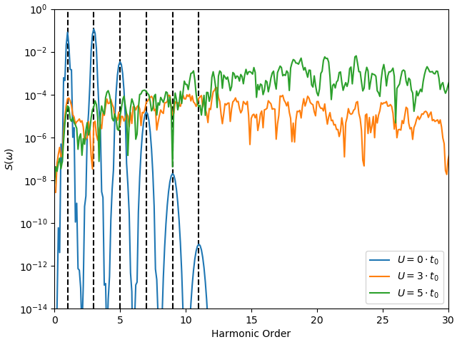
The response of a given material to optical stimulation depends heavily on the values of and that define the material’s electronic properties. For Mott insulators, charge is carried by doublon-hole excitations [60], the pair production of which decreases exponentially with [64]. Fig. 1 show some of the essential optical characteristics resulting from this, such as a white light response to optical driving in sufficiently strong Mott insulators. In the conducting limit, the spectral behaviour becomes identical to atomic systems [67], with well defined peaks present at odd harmonics.
There is no simple method for determining the effect of on material response, but we can obtain a heuristic understanding of how this factor affects optical spectra in the limit of large . Taking , the propagator will be of the form:
| (8) |
We would like to approximate an effective time-independent Hamiltonian, such that:
| (9) |
can be expressed in terms of the Magnus expansion [68]:
| (10) |
The first term in this expansion is given by
| (11) |
The integral over the two body term of Eq.(1) is trivial given that it is time independent. Thus, we focus our attention on the integral over the hopping term:
| (12) | ||||
| (13) |
where integrating over the duration of the single pulse, . The relevant integral is therefore
| (14) |
where .
In order to restrict the analysis to this first order term, we treat the scaling factor as a large parameter, meaning higher order terms in the Magnus expansion will oscillate rapidly and can be neglected. Given the envelope is slowly varying relative to , for each half period , we approximate it by its averaged value over that period:
| (15) |
Consequently, the integral can be approximated as
| (16) |
where is the zero order Bessel function [69, Eq. (10.9.1)]. In the limit of large , this function may be replaced by its asymptote [69, Eq. (10.17.3)] to obtain
| (17) |
where
| (18) |
Having approximated the integral, it is now possible to state the form of the effective Hamiltonian in Eq. (9):
| (19) |
This effective Hamiltonian is in the form of the Hubbard Hamiltonian in equilibrium with one important difference, the scaling of the hopping energy by .
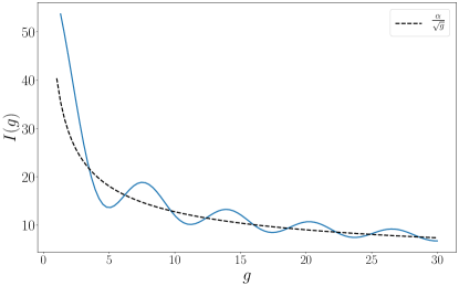
Note that while has some dependence, this occurs only in the trigonometric terms in the sum, meaning that this parameter will be bounded with respect to , and have little impact once the response is normalised. This is borne out by numerical calculation of Eq.(14), as shown in Fig. 3. Here it is apparent that the contribution of at large is the introduction of small oscillations around . It therefore follows that the principal effect of increasing will be the scaling of the system response in the following manner:
| (20) |
Clearly, for any insulator, the effective ratio of the interaction parameter to the hopping parameter is proportional to the scaling parameter, so an increase in leads to a higher effective ratio, one where dominates the dynamics of the system. Consequently, increasing means all systems are shifted towards the high , strongly insulating regime. The one exception to this is the conducting system, which will only experience a scaling in the magnitude of its optical response, rather than its dynamical character.
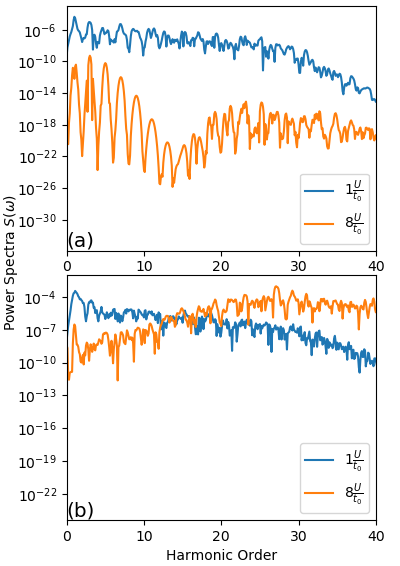
Thus, when is increased, we expect that the distance between the responses of two Mott insulators given by Eqs. (4) and (5) to reduce, regardless of the specific ratio corresponding to each system. This is exactly the phenomena illustrated in Fig. 4: at low scaling the two systems have highly distinguishable responses, but at high scaling their power spectra are more similar. The only type of material that will be distinguishable from Mott insulators in the high regime are conductors whose response is unaffected by the scaling in Eq. (20).
III Results
In this section, we numerically investigate the extent to which the degree of distinguishability between systems depends on both system , and pulse parameters and . In particular, we demonstrate that there is a comparatively high experimental optical discriminability between many Mott insulators at a low lattice spacing and low field strength relative to the driving frequency. Conversely, as predicted in Sec.II, as one increases the factor , all systems (except conductors) exhibit behaviour associated with the large regime, and hence become less distinguishable. The increased distinguishability of conductors in this parameter range is also demonstrated.
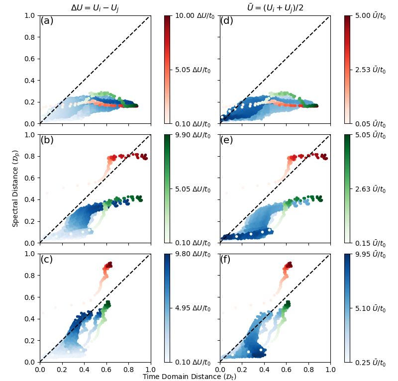
Pairs of systems distinguished by potentials and are simulated via exact diagonalization in QuSpin [70]. From this, the distance measures of Eqs.(4,5) are calculated. These distances are then scaled to their maximum value over the total range of parameter pairs considered, to give a measure of relative distinguishability. Fig. 5 summarises these results, reporting relative distinguishability in the time and spectral domains via both the difference and average of each system’s potential.
The first point to note is that in almost all cases, the relative distinguishability of two systems is greater in the time domain than the spectral domain (i.e. points lie below the diagonal), demonstrating the importance of phase information for distinguishing between system responses. As might be expected, distinguishability tends to be lowest for materials with small and high . The relative distinguishability between the two domains also changes dramatically as is increased.
The clearest example of this is in the behaviour of system pairs where one system is a conductor (). In this case, while the time domain distinguishability is reduced with higher field amplitudes, the spectral distinguishability increases significantly, such that at high driving fields spectral characteristics provide a greater degree of distinguishability compared to the time domain.
In fact, when examining both difference and average, a clear trend that emerges where systems close to the conducting limit increase in spectral distinguishability as increases. This is to be expected, given the scaling argument in Eq. (20). Since the effective ratio of conductors cannot be scaled by the field strength or lattice constant, conductor response to optical driving remains is only scaled, rather than dynamically changed by varying . A system close to this limit will still retain its conductor-like properties, whereas a system that is already deeply in the insulating regime is scaled into an even more strongly insulating system. This behaviour is most strikingly observed in Fig. 5 c), where at high a banding effect is observed separating distinguishabilities into those systems where one of the material pair is either a conductor or small material.
Finally, we find in all cases that while increasing may increase spectral distinguishability, for almost all pairs in the time domain, a steady compression of distinguishability along this axis can be observed, as one might expect from Eq.(20). This is itself strongly dependent on , with a relatively small subset of pairs featuring both high and small becoming relatively more distinguishable in the spectral domain than the time domain at high (i.e. Fig. 5 c) and f)).
IV Discussion
Here we have examined the feasibility of distinguishing driven Mott insulators via their optical response. Simulation demonstrated that the importance of phase information in this process was dependent on the applied field strength, and confirmed the heuristic argument that the distinguishability of insulators should decrease as the field strength is increased. To paraphrase Tolstoy [71], conductors - like happy families - always retain a high degree of distinguishability in one domain or another, whereas the distinguishability of insulating pairs depends strongly on the driving field amplitude.
The high dependence of material response on the scaling factor begs the question, what scaling values are physically realizable for high frequency pulses? Considering a simple subclass of Mott insulators, transition metal oxides, we determine that 4 Å is physically realistic lattice constant based on studies performed by Heine and Mattheiss [72]. Hohenleutner et al. [36] also experimentally demonstrated pulse generation with a peak field of 44 . Thus, given an infrared frequency THz, the scaling factors studied here are certainly within the range of allowed experimental values, since these estimates place a maximum scaling at . Moreover, the results presented here demonstrate that the change in distinguishability sweeping over a range of field strengths may also serve as a useful source of information for identifying materials.
It is rather interesting to note that the strong dependence of distinguishability on implies that the Keldysh parameter may also serve as a proxy for optical distinguishability for systems. Indeed, given this parameter will depend on each system’s correlation length (and therefore ), it encapsulates more information about each system individually than alone. A potential future avenue of investigation would there be to study whether a pairwise function of each system’s may offer some predictive heuristic for their relative distinguishability.
Of particular importance is the finding that experimental differentiation between different Mott insulators is in most cases more easily achieved in the time domain. While spectral characteristics are unquestionably easier to obtain experimentally, the results presented show that the technique of THz time domain spectroscopy [73, 74] could profitably be employed to better distinguish between materials.
Though our results only apply to strongly-correlated materials, sufficient experimental optical similarity between a known Mott insulator whose atoms are spaced sufficiently and a material with comparable interatomic spacing could provide an aid to the nontrivial problem of distinguishing between a band insulator and a Mott insulator [53].
Acknowledgements.
This work has been generously supported by Army Research Office (ARO) (grant W911NF-19-1-0377; program manager Dr. James Joseph). J.M. was supported by the ARO Undergraduate Research Apprenticeship Program and the Tulane Honors Summer Research Program. The views and conclusions contained in this document are those of the authors and should not be interpreted as representing the official policies, either expressed or implied, of ARO or the U.S. Government. The U.S. Government is authorized to reproduce and distribute reprints for Government purposes notwithstanding any copyright notation herein.References
- Franken et al. [1961] P. A. Franken, A. E. Hill, C. W. Peters, and G. Weinreich, Generation of optical harmonics, Phys. Rev. Lett. 7, 118 (1961).
- Kaiser and Garrett [1961] W. Kaiser and C. G. B. Garrett, Two-photon excitation in ca: , Phys. Rev. Lett. 7, 229 (1961).
- Dowling and Milburn [2003] J. P. Dowling and G. J. Milburn, Quantum technology: the second quantum revolution, Philosophical Transactions of the Royal Society of London. Series A: Mathematical, Physical and Engineering Sciences 361, 1655 (2003).
- Rothman et al. [2005] A. Rothman, T.-S. Ho, and H. Rabitz, Observable-preserving control of quantum dynamics over a family of related systems, Phys. Rev. A 72, 023416 (2005).
- Magann et al. [2018] A. Magann, T.-S. Ho, and H. Rabitz, Singularity-free quantum tracking control of molecular rotor orientation, Phys. Rev. A 98, 043429 (2018).
- Campos et al. [2017] A. G. Campos, D. I. Bondar, R. Cabrera, and H. A. Rabitz, How to Make Distinct Dynamical Systems Appear Spectrally Identical, Phys. Rev. Lett. 118, 083201 (2017).
- McCaul et al. [2020a] G. McCaul, C. Orthodoxou, K. Jacobs, G. H. Booth, and D. I. Bondar, Driven imposters: Controlling expectations in many-body systems, Phys. Rev. Lett. 124, 183201 (2020a).
- McCaul et al. [2020b] G. McCaul, C. Orthodoxou, K. Jacobs, G. H. Booth, and D. I. Bondar, Controlling arbitrary observables in correlated many-body systems, Phys. Rev. A 101, 053408 (2020b).
- Busson and Tadjeddine [2009] B. Busson and A. Tadjeddine, Non-uniqueness of parameters extracted from resonant second-order nonlinear optical spectroscopies, Journal of Physical Chemistry C 113, 21895 (2009).
- McCaul et al. [2021a] G. McCaul, A. F. King, and D. I. Bondar, Optical indistinguishability via twinning fields, Phys. Rev. Lett. 127, 113201 (2021a).
- Ong et al. [1984] C. K. Ong, G. M. Huang, T. J. Tarn, and J. W. Clark, Invertibility of quantum-mechanical control systems, Mathematical systems theory 17, 335 (1984).
- Clark et al. [1985] J. W. Clark, C. K. Ong, T. J. Tarn, and G. M. Huang, Quantum nondemolition filters, Mathematical systems theory 18, 33 (1985).
- Jha et al. [2009] A. Jha, V. Beltrani, C. Rosenthal, and H. Rabitz, Multiple Solutions in the Tracking Control of Quantum Systems, The Journal of Physical Chemistry A 113, 7667 (2009).
- McCaul et al. [2021b] G. McCaul, A. F. King, and D. I. Bondar, Non-uniqueness of non-linear optical response (2021b), arXiv:2110.06189 .
- Chiao et al. [1964] R. Y. Chiao, E. Garmire, and C. H. Townes, Self-trapping of optical beams, Phys. Rev. Lett. 13, 479 (1964).
- Kroner et al. [2008] M. Kroner, A. O. Govorov, S. Remi, B. Biedermann, S. Seidl, A. Badolato, P. M. Petroff, W. Zhang, R. Barbour, B. D. Gerardot, R. J. Warburton, and K. Karrai, The nonlinear fano effect, Nature 451, 311 (2008).
- Shen [1984] Y.-R. Shen, Principles of nonlinear optics (Wiley-Interscience, New York, NY, USA, 1984).
- de Araújo et al. [2016] C. B. de Araújo, A. S. L. Gomes, and G. Boudebs, Techniques for nonlinear optical characterization of materials: a review, Reports on Progress in Physics 79, 036401 (2016).
- Boyd [2008] R. W. Boyd, Nonlinear optics, 3rd ed. (Academic Press, Amsterdam ; Boston, 2008).
- Itatani et al. [2004] J. Itatani, J. Levesque, D. Zeidler, H. Niikura, H. Pépin, J. C. Kieffer, P. B. Corkum, and D. M. Villeneuve, Tomographic imaging of molecular orbitals, Nature 432, 867 (2004).
- Hay et al. [2002] N. Hay, R. Velotta, M. Lein, R. de Nalda, E. Heesel, M. Castillejo, and J. P. Marangos, High-order harmonic generation in laser-aligned molecules, Phys. Rev. A 65, 053805 (2002).
- Lein et al. [2002a] M. Lein, N. Hay, R. Velotta, J. P. Marangos, and P. L. Knight, Interference effects in high-order harmonic generation with molecules, Phys. Rev. A 66, 023805 (2002a).
- Lein et al. [2003] M. Lein, P. P. Corso, J. P. Marangos, and P. L. Knight, Orientation dependence of high-order harmonic generation in molecules, Phys. Rev. A 67, 023819 (2003).
- Kamta and Bandrauk [2004] G. L. Kamta and A. D. Bandrauk, High-order harmonic generation from two-center molecules: Time-profile analysis of nuclear contributions, Phys. Rev. A 70, 011404 (2004).
- Kamta and Bandrauk [2005] G. L. Kamta and A. D. Bandrauk, Three-dimensional time-profile analysis of high-order harmonic generation in molecules: Nuclear interferences in , Phys. Rev. A 71, 053407 (2005).
- Eidi et al. [2021] M. Eidi, M. Vafaee, H. Koochaki Kelardeh, and A. Landsman, High-order harmonic generation by static coherent states method in single-electron atomic and molecular systems, Journal of Computational Chemistry 42, 1312 (2021), https://onlinelibrary.wiley.com/doi/pdf/10.1002/jcc.26549 .
- von der Linde et al. [1995] D. von der Linde, T. Engers, G. Jenke, P. Agostini, G. Grillon, E. Nibbering, A. Mysyrowicz, and A. Antonetti, Generation of high-order harmonics from solid surfaces by intense femtosecond laser pulses, Phys. Rev. A 52, R25 (1995).
- Dromey et al. [2006] B. Dromey, M. Zepf, A. Gopal, K. Lancaster, M. S. Wei, K. Krushelnick, M. Tatarakis, N. Vakakis, S. Moustaizis, R. Kodama, M. Tampo, C. Stoeckl, R. Clarke, H. Habara, D. Neely, S. Karsch, and P. Norreys, High harmonic generation in the relativistic limit, Nature Physics 2, 456 (2006).
- Vampa et al. [2014] G. Vampa, C. R. McDonald, G. Orlando, D. D. Klug, P. B. Corkum, and T. Brabec, Theoretical analysis of high-harmonic generation in solids, Phys. Rev. Lett. 113, 073901 (2014).
- Kruchinin et al. [2018] S. Y. Kruchinin, F. Krausz, and V. S. Yakovlev, Colloquium: Strong-field phenomena in periodic systems, Rev. Mod. Phys. 90, 021002 (2018).
- Ortmann and Landsman [2021] L. Ortmann and A. S. Landsman, Chapter Two - High-harmonic generation in solids (Academic Press, 2021) pp. 103–156.
- Ghimire et al. [2011] S. Ghimire, A. D. DiChiara, E. Sistrunk, P. Agostini, L. F. DiMauro, and D. A. Reis, Observation of high-order harmonic generation in a bulk crystal, Nature Physics 7, 138 (2011).
- Vampa et al. [2015] G. Vampa, T. J. Hammond, N. Thiré, B. E. Schmidt, F. Légaré, C. R. McDonald, T. Brabec, and P. B. Corkum, Linking high harmonics from gases and solids, Nature 522, 462 (2015).
- Ndabashimiye et al. [2016] G. Ndabashimiye, S. Ghimire, M. Wu, D. A. Browne, K. J. Schafer, M. B. Gaarde, and D. A. Reis, Solid-state harmonics beyond the atomic limit, Nature 534, 520 (2016).
- Luu et al. [2015] T. T. Luu, M. Garg, S. Y. Kruchinin, A. Moulet, M. T. Hassan, and E. Goulielmakis, Extreme ultraviolet high-harmonic spectroscopy of solids, Nature 521, 498 (2015).
- Hohenleutner et al. [2015] M. Hohenleutner, F. Langer, O. Schubert, M. Knorr, U. Huttner, S. W. Koch, M. Kira, and R. Huber, Real-time observation of interfering crystal electrons in high-harmonic generation, Nature 523, 572 (2015).
- Langer et al. [2016] F. Langer, M. Hohenleutner, C. P. Schmid, C. Poellmann, P. Nagler, T. Korn, C. Schüller, M. S. Sherwin, U. Huttner, J. T. Steiner, S. W. Koch, M. Kira, and R. Huber, Lightwave-driven quasiparticle collisions on a subcycle timescale, Nature 533, 225 (2016).
- Yoshikawa et al. [2017] N. Yoshikawa, T. Tamaya, and K. Tanaka, High-harmonic generation in graphene enhanced by elliptically polarized light excitation, Science 356, 736 (2017), https://science.sciencemag.org/content/356/6339/736.full.pdf .
- Liu et al. [2017] H. Liu, Y. Li, Y. S. You, S. Ghimire, T. F. Heinz, and D. A. Reis, High-harmonic generation from an atomically thin semiconductor, Nature Physics 13, 262 (2017).
- You et al. [2017] Y. S. You, D. Reis, and S. Ghimire, Anisotropic high-harmonic generation in bulk crystals, Nature Physics 13, 345 (2017).
- Huttner et al. [2017] U. Huttner, M. Kira, and S. W. Koch, Ultrahigh off-resonant field effects in semiconductors, Laser & Photonics Reviews 11, 1700049 (2017), https://onlinelibrary.wiley.com/doi/pdf/10.1002/lpor.201700049 .
- Ciappina et al. [2017] M. F. Ciappina, J. A. Pérez-Hernández, A. S. Landsman, W. A. Okell, S. Zherebtsov, B. Förg, J. Schötz, L. Seiffert, T. Fennel, T. Shaaran, T. Zimmermann, A. Chacón, R. Guichard, A. Zaïr, J. W. G. Tisch, J. P. Marangos, T. Witting, A. Braun, S. A. Maier, L. Roso, M. Krüger, P. Hommelhoff, M. F. Kling, F. Krausz, and M. Lewenstein, Attosecond physics at the nanoscale, Reports on Progress in Physics 80, 54401 (2017).
- Drescher et al. [2001] M. Drescher, M. Hentschel, R. Kienberger, G. Tempea, C. Spielmann, G. A. Reider, P. B. Corkum, and F. Krausz, X-ray pulses approaching the attosecond frontier, Science 291, 1923 (2001), https://science.sciencemag.org/content/291/5510/1923.full.pdf .
- Paul et al. [2001] P. M. Paul, E. S. Toma, P. Breger, G. Mullot, F. Augé, P. Balcou, H. G. Muller, and P. Agostini, Observation of a train of attosecond pulses from high harmonic generation, Science 292, 1689 (2001), https://science.sciencemag.org/content/292/5522/1689.full.pdf .
- Hentschel et al. [2001] M. Hentschel, R. Kienberger, C. Spielmann, G. A. Reider, N. Milosevic, T. Brabec, P. Corkum, U. Heinzmann, M. Drescher, and F. Krausz, Attosecond metrology, Nature 414, 509 (2001).
- Krausz and Ivanov [2009] F. Krausz and M. Ivanov, Attosecond physics, Rev. Mod. Phys. 81, 163 (2009).
- Landsman and Keller [2015] A. S. Landsman and U. Keller, Attosecond science and the tunnelling time problem, Physics Reports 547, 1 (2015), attosecond science and the tunneling time problem.
- Magann et al. [2022] A. B. Magann, G. McCaul, H. A. Rabitz, and D. I. Bondar, Sequential optical response suppression for chemical mixture characterization, Quantum 6, 626 (2022), arXiv:2010.13859 .
- Krausz [2001] F. Krausz, From femtochemistry to attophysics, Physics World 14, 41 (2001).
- Cireasa et al. [2015] R. Cireasa, A. E. Boguslavskiy, B. Pons, M. C. H. Wong, D. Descamps, S. Petit, H. Ruf, N. Thiré, A. Ferré, J. Suarez, J. Higuet, B. E. Schmidt, A. F. Alharbi, F. Légaré, V. Blanchet, B. Fabre, S. Patchkovskii, O. Smirnova, Y. Mairesse, and V. R. Bhardwaj, Probing molecular chirality on a sub-femtosecond timescale, Nature Physics 11, 654 (2015).
- Neufeld et al. [2019] O. Neufeld, D. Ayuso, P. Decleva, M. Y. Ivanov, O. Smirnova, and O. Cohen, Ultrasensitive chiral spectroscopy by dynamical symmetry breaking in high harmonic generation, Phys. Rev. X 9, 031002 (2019).
- Jiménez-Galán et al. [2021] Á. Jiménez-Galán, R. E. Silva, O. Smirnova, and M. Ivanov, Sub-cycle valleytronics: control of valley polarization using few-cycle linearly polarized pulses, Optica 8, 277 (2021).
- Lee et al. [2021] J. Lee, K.-H. Jin, and H. W. Yeom, Distinguishing a mott insulator from a trivial insulator with atomic adsorbates, Phys. Rev. Lett. 126, 196405 (2021).
- Chergui and Zewail [2009] M. Chergui and A. H. Zewail, Electron and x-ray methods of ultrafast structural dynamics: Advances and applications, ChemPhysChem 10, 28 (2009), https://chemistry-europe.onlinelibrary.wiley.com/doi/pdf/10.1002/cphc.200800667 .
- Lein et al. [2002b] M. Lein, N. Hay, R. Velotta, J. P. Marangos, and P. L. Knight, Role of the intramolecular phase in high-harmonic generation, Phys. Rev. Lett. 88, 183903 (2002b).
- Shao et al. [2022] C. Shao, H. Lu, X. Zhang, C. Yu, T. Tohyama, and R. Lu, High-harmonic generation approaching the quantum critical point of strongly correlated systems, Phys. Rev. Lett. 128, 047401 (2022).
- Garg et al. [2021] M. Garg, A. Martin-Jimenez, M. Pisarra, Y. Luo, F. Martín, and K. Kern, Real-space subfemtosecond imaging of quantum electronic coherences in molecules, Nature Photonics 10.1038/s41566-021-00929-1 (2021).
- Simon [2013] S. H. Simon, The Oxford solid state basics (OUP Oxford, 2013).
- Essler et al. [2005] F. Essler, H. Frahm, F. Gohmann, A. Klumper, and V. Korepin, The One-Dimensional Hubbard Model (Cambridge University Press, 2005).
- Murakami et al. [2018] Y. Murakami, M. Eckstein, and P. Werner, High-harmonic generation in mott insulators, Phys. Rev. Lett. 121, 057405 (2018).
- Imai et al. [2020] S. Imai, A. Ono, and S. Ishihara, High harmonic generation in a correlated electron system, Phys. Rev. Lett. 124, 157404 (2020).
- Silva et al. [2018] R. E. F. Silva, I. V. Blinov, A. N. Rubtsov, O. Smirnova, and M. Ivanov, High-harmonic spectroscopy of ultrafast many-body dynamics in strongly correlated systems, Nature Photonics 12, 266 (2018).
- Ashcroft and Mermin [1976] N. Ashcroft and N. Mermin, Solid State Physics (Saunders College, Philadelphia, 1976).
- Oka [2012] T. Oka, Nonlinear doublon production in a mott insulator: Landau-dykhne method applied to an integrable model, Phys. Rev. B 86, 075148 (2012).
- Keldysh et al. [1965] L. Keldysh et al., Ionization in the field of a strong electromagnetic wave, Sov. Phys. JETP 20, 1307 (1965).
- Stafford et al. [1991] C. A. Stafford, A. J. Millis, and B. S. Shastry, Finite-size effects on the optical conductivity of a half-filled hubbard ring, Phys. Rev. B 43, 13660 (1991).
- Krause et al. [1992] J. L. Krause, K. J. Schafer, and K. C. Kulander, High-order harmonic generation from atoms and ions in the high intensity regime, Phys. Rev. Lett. 68, 3535 (1992).
- Blanes et al. [2009] S. Blanes, F. Casas, J. Oteo, and J. Ros, The magnus expansion and some of its applications, Physics Reports 470, 151–238 (2009).
- [69] DLMF, NIST Digital Library of Mathematical Functions, http://dlmf.nist.gov/, Release 1.1.3 of 2021-09-15, f. W. J. Olver, A. B. Olde Daalhuis, D. W. Lozier, B. I. Schneider, R. F. Boisvert, C. W. Clark, B. R. Miller, B. V. Saunders, H. S. Cohl, and M. A. McClain, eds.
- Weinberg and Bukov [2019] P. Weinberg and M. Bukov, QuSpin: a Python Package for Dynamics and Exact Diagonalisation of Quantum Many Body Systems. Part II: bosons, fermions and higher spins, SciPost Phys. 7, 20 (2019).
- Tolstoy [2013] L. Tolstoy, Anna Karenina : a novel in eight parts (Penguin Classics, London, 2013).
- Heine and Mattheiss [1971] V. Heine and L. F. Mattheiss, Metal-insulator transition in transition metal oxides, Journal of Physics C: Solid State Physics 4, L191 (1971).
- Dorney et al. [2001] T. D. Dorney, R. G. Baraniuk, and D. M. Mittleman, Material parameter estimation with terahertz time-domain spectroscopy, J. Opt. Soc. Am. A 18, 1562 (2001).
- Neu and Schmuttenmaer [2018] J. Neu and C. A. Schmuttenmaer, Tutorial: An introduction to terahertz time domain spectroscopy (thz-tds), Journal of Applied Physics 124, 231101 (2018), https://doi.org/10.1063/1.5047659 .