Subsurface distances for hyperbolic $3$–manifolds fibering over the circle

Abstract.

For a hyperbolic fibered $3$–manifold $M$, we prove results that uniformly relate the structure of surface projections as one varies the fibrations of $M$. This extends our previous work from the fully-punctured to the general case.

1. Introduction

Let $M$ be a hyperbolic $3$-manifold and let $S$ be a fiber in a fibration of $M$ over the circle. The corresponding monodromy is a pseudo-Anosov homeomorphism $\phi\colon S\to S$ and comes equipped with invariant stable and unstable laminations $\lambda^{\pm}$ on $S$. Let $N_{S}\to M$ be the infinite cyclic covering of $M$ corresponding to $S$.

As a consequence of the proof of Thurston’s Ending Lamination Conjecture, Minsky [Min10] and Brock–Canary–Minsky [BCM12] develop combinatorial tools to study the geometry of a hyperbolic manifold homeomorphic to $S\times\mathbb{R}$. Applying their work to the special case of $N_{S}\cong S\times\mathbb{R}$ explains how the geometry of $N_{S}$, and hence that of $M$, is coarsely determined by combinatorial data associated to the pair of laminations $\lambda^{\pm}$. In particular, using only the pair $\lambda^{\pm}$, a combinatorial model of $N_{S}$ (called the model manifold) is constructed and this model is shown to be biLipschitz to $N_{S}$, where the biLipschitz constant depends only on the complexity of the surface $S$. For this, one of the main combinatorial tools are the Masur–Minsky subsurface projections [MM00], which associate to each subsurface $Y\subset S$ a subsurface projection distance $d_{Y}(\lambda^{-},\lambda^{+})$ measuring the complexity of $\lambda^{\pm}$ as seen from $Y$. In fact, subsurface projections have proven to be useful in several settings [Raf07, BKMM12, MS13] and have been generalized in many directions [BBF15, BF14, BHS17, ST19].

These developments suggest the following outline for studying the geometry of a hyperbolic fibered $3$-manifold $M$: apply the model manifold machinery to an infinite cyclic cover of $M$ associated to a fiber and use this to make conclusions about the structure of $M$. In fact, because of Agol’s resolution of the Virtual Fibering Conjecture [AGM13], this simple idea generalizes to any hyperbolic manifold by first passing to a finite sheeted cover which fibers over the circle.

Unfortunately, this approach is too naïve for a number of reasons, perhaps the most important of which is that the complexity of a fiber in the appropriate cover is not known at the outset. Indeed, even when a fibered manifold $M$ is fixed, if $\mathrm{dim}(H^{1}(M;\mathbb{R}))\geq 2$ then $M$ fibers in infinitely many ways, and the complexities of the corresponding fibers are necessarily unbounded. Since the bilipschitz constants in the Model Manifold Theorem depend on the complexity of the underlying surface, this approach goes nowhere without a precise understanding of how the constants relating geometry to combinatorics vary as the surface changes.

To salvage this approach, one would like control over how the tools at the center of the construction depend on complexity. The purpose of this paper is to give such uniform, explicit control on subsurface projection distances as one varies the fibers within a fixed fibered manifold. This extends our previous work [MT17] that handled the special case of fully-punctured fibered manifolds (see below for details).

Main results

Recall that the fibrations of a manifold $M$ are organized into finitely many “fibered faces” of the unit ball in $H^{1}(M,\mathbb{R})$ of the Thurston norm [Thu86], where each fibered face $\bf F$ has the property that all primitive integral classes in the open cone $\mathbb{R}_{+}\bf F$ represent a fiber (see Section 2.3). Associated to each fibered face is a pseudo-Anosov flow which is transverse to every fiber represented in $\mathbb{R}_{+}\bf F$ [Fri82].

Our first main result bounds the size and projection distance for all subsurfaces of all fibers over a fixed fibered face $\bf F$. The constant $D$ in the statement is no more than $15$ (see Section 2.1.2) and $|\chi^{\prime}(Y)|=\max\{|\chi(Y)|,1\}$.

Theorem 1.1 (Bounding projections for $M$).

Let $M$ be a hyperbolic fibered $3$-manifold with fibered face $\bf F$. Then for any fiber $S$ contained in $\mathbb{R}_{+}\bf F$ and any subsurface $Y$ of $S$

$$|\chi^{\prime}(Y)|\cdot\big{(}d_{Y}(\lambda^{-},\lambda^{+})-16D\big{)}\leq 2D\>|\bf F|,$$

where $|\bf F|$ is a constant depending only on $\bf F$.

In particular, subsurface projections are uniformly bounded over the fibered face $\bf F$ as are the complexities of subsurfaces whose projection distances are greater than $16D$. Note that since $M$ has only finitely many fibered faces, this bounds the size of all subsurface projections among all fibers of $M$.

Second, we relate subsurfaces of different fibers in the same fibered face of $M$. Note that here the constants involved do not depend on the manifold $M$.

Theorem 1.2 (Subsurface dichotomy).

Let $M$ be a hyperbolic fibered $3$-manifold and let $S$ and $F$ be fibers of $M$ which are contained in the same fibered cone. If $W\subset F$ is a subsurface of $F$ then either $W$ is homotopic, through surfaces transverse to the associated flow, to an embedded subsurface $W^{\prime}$ of $S$ with

$$d_{W^{\prime}}(\lambda^{-},\lambda^{+})=d_{W}(\lambda^{-},\lambda^{+})$$

or the fiber $S$ satisfies

$$9D\cdot|\chi(S)|\geq d_{W}(\lambda^{-},\lambda^{+})-16D.$$

Along the way to establishing our main theorems, we prove several results that may be independently interesting. While most of these concern the connection between the manifold $M$ and the veering triangulation of the associated fully-punctured manifold (see the next section for details), we also obtain information about subsurface projections to immersed subsurfaces.

For a finitely generated subgroup $\Gamma<\pi_{1}(S)$, let $S_{\Gamma}\to S$ be the corresponding cover. If $Y\subset S_{\Gamma}$ is a compact core, the covering map restricted to $Y$ is an immersion and we say that $Y\to S$ corresponds to $\Gamma<\pi_{1}(S)$. Lifting to the cover induces a (partially defined) map of curve and arc graphs which we denote $\pi_{Y}\colon\mathcal{A}(S)\to\mathcal{A}(Y)$. (When $\Gamma$ is cyclic, we set $\mathcal{A}(Y)$ to be the annular curve graph $\mathcal{A}(S_{\Gamma})$ as usual.) Note that these constructions depend on $\Gamma$ but not on the choice of $Y$ and that $\pi_{Y}$ agrees with the usual subsurface projection when $Y\subset S$ is an embedded subsurface.

Theorem 1.3 (Immersions to covers).

There is a constant $M\leq 38$ satisfying the following: Let $S$ be a surface and let $Y\to S$ be an immersion corresponding to a finitely generated $\Gamma<\pi_{1}(S)$. Then either

• there is a subsurface $W\subset S$ so that $Y\to S$ factors (up to homotopy) through a finite sheeted covering $Y\to W$, or

• the diameter of the entire projection of $\mathcal{A}(S)$ to $\mathcal{A}(Y)$ is bounded by $M$.

The novelty of Theorem 1.3 is that the constant $M\leq 38$ is explicit and uniform over all surfaces and immersions. Previously, Rafi and Schleimer proved that for any finite cover $\widetilde{S}\to S$ there is a constant $T\geq 0$ (depending on $\widetilde{S}$ and $S$) such that if $Y\subset\widetilde{S}$ is a subsurface with $d_{Y}(\alpha,\beta)\geq T$ for $\alpha,\beta\in\mathcal{A}(S)$, then $Y$ covers a subsurface of $S$ [RS09, Lemma 7.2].

Relation to our previous work

Given a fibered face $\bf F$ of $M$ and its associated pseudo-Anosov flow, the stable/unstable laminations $\Lambda^{\pm}$ of the flow intersect each fiber to give the laminations associated to its monodromy. Removing the singular orbits of the flow produces the fully-punctured manifold $\mathring{M}$ associated to the face $\bf F$. If $\phi\colon S\to S$ is the monodromy of some fiber $S$ representing a class in $\mathbb{R}_{+}\bf F$, then $\mathring{M}$ is the mapping torus of the surface $\mathring{S}$ obtained from $S$ by puncturing at the singularities of $\phi$. The fibered face of $\mathring{M}$ containing $\mathring{S}$ is denoted $\mathring{\bf F}$ and the inclusion $\mathring{M}\subset M$ induces an injective homomorphism $H^{1}(M\;\mathbb{R})\hookrightarrow H^{1}(\mathring{M}\;\mathbb{R})$ mapping $\mathbb{R}_{+}\bf F$ into $\mathbb{R}_{+}\mathring{\bf F}$.

In our previous work [MT17], we restricted our study of subsurface projections in fibered manifolds to the fully-punctured settings. When $\mathring{M}$ is fully-punctured, it admits a canonical veering triangulation $\tau$ [Ago11, Gué16] associated to the fibered face $\mathring{\bf F}$. We found that the combinatorial structure of this triangulation encodes the hierarchy of subsurface projections for each fiber $\mathring{F}$ in $\mathbb{R}_{+}\mathring{\bf F}$. As a result, we established versions of Theorems 1.1 and 1.2 in that restricted setting (though with better constants than available in general). In fact, when the fibered manifold is fully-punctured there are additional surprising connections between the veering triangulation and the curve graph. For example, a fiber $\mathring{F}$ of $\mathring{M}$ is necessarily a punctured surface, and edges of the triangulation $\tau$ (when lifted to the cover of $\mathring{M}$ corresponding to $\mathring{F}$) form a subset of the arc graph $\mathcal{A}(\mathring{F})$. This subset is geodesically connected in the sense that for any pair of arcs of $\mathring{F}$ coming from edges of $\tau$ there is a geodesic in $\mathcal{A}(\mathring{F})$ joining them consisting entirely of veering edges [MT17, Theorem 1.4]. Such a result cannot have a precise analog if, for example, the manifold $M$ is closed.

In this paper, we extend our study to general (e.g. closed) hyperbolic fibered manifolds. The main difficulty here is that these manifolds do not admit veering triangulations. So our approach is to start with an arbitrary fibered manifold $M$ and consider the veering triangulation of the associated fully-punctured manifold $\mathring{M}$. (For example, the constant $|\bf F|$ appearing in Theorem 1.1 is precisely the number of tetrahedra of the veering triangulation of $\mathring{M}$ associated to $\mathring{\bf F}$.) Unfortunately, results about subsurface projections to fibers of $M$ do not directly imply the corresponding statements in $\mathring{M}$. Instead, we develop tools to relate sections of the veering triangulation (i.e. ideal triangulations of the fully-punctured fiber by edges of the veering triangulation) to subsurface projections in the fibers of $M$.

Summary of paper

In Section 2 we present background material. In particular, we summarize the definition of the veering triangulation (Section 2.2) and recall the main constructions from [MT17] that connect the structure of the veering triangulation on $\mathring{S}\times\mathbb{R}$ to subsurface representatives in $\mathring{S}$ (Section 2.4).

Section 3 introduces the lattice structure of sections of the veering triangulation. It concludes with Section 3.2 which details how sections (which are ideal triangulations of the fully-punctured surface $\mathring{S}$) are used to define projections to the curve graph of subsurfaces of the original surface $S$. This is followed by Section 4 where Theorem 1.3 is proven. This section does not use veering triangulations and can be read independently from the rest of the paper.

In Section 5, we prove two estimates that relate the veering triangulation of the fully-punctured manifold $\mathring{M}$ to fibers of $M$. The first (Proposition 5.1) shows that for each subsurface $Y$ of $S$, there are top and bottom sections of $\mathring{S}\times\mathbb{R}$ which project close to the images of $\lambda^{\pm}$ in $\mathcal{A}(Y)$. The second (Lemma 5.2) shows that these projections to $\mathcal{A}(Y)$ move slowly from $\pi_{Y}(\lambda^{-})$ to $\pi_{Y}(\lambda^{+})$ depending on the size of $Y$. Both of these estimates are needed for proofs of Theorems 1.1 and 1.2.

Finally, in Sections 6 and 7, Theorems 1.1 and 1.2 are proven. The bulk of the proof of Theorem 1.1 involves building a simplicial pocket for the subsurface $Y$ that embeds into the veering triangulation of $\mathring{M}$ whose “width” is approximately $|\chi(Y)|$ and whose “depth” is at least $d_{Y}(\lambda^{-},\lambda^{+})$. For Theorem 1.2, we show that if a subsurface $W$ of a fiber $F$ is not homotopic into another fiber $S$ (in the same fibered cone) then, after puncturing along singular orbits of the flow, a section (triangulation) of $\mathring{S}$ contains many edges, proportional to the “depth” of the pocket for $W$. For each of these arguments, the difficulty lies in the fact that we are extracting information about the original manifold $M$ and projections to subsurfaces of its fibers by relying on the veering triangulation of $\mathring{M}$, which a priori only records information about projections to its fully-punctured fibers.

Acknowledgments

Minsky was partially supported by NSF grants DMS-1610827 and DMS-2005328, and Taylor was partially supported by NSF grants DMS-1744551 and DMS-2102018 and the Sloan Foundation.

2. Background

Here we record basic background that we will need throughout the paper. We begin with some material that follows easily from standard facts about curve graphs and then recall the definition of the veering triangulation. We conclude by reviewing results from [MT17] which develop connections between the two.

2.1. Curve graph facts and computations

The arc and curve graph $\mathcal{A}(Y)$ for a compact surface $Y$ is the graph whose vertices are homotopy classes of essential simple closed curves and proper arcs. Edges join vertices precisely when the vertices have disjoint representatives on $Y$. Here, essential curves/arcs are those which are not homotopic (rel endpoints) to a point or into the boundary.

If $Y$ is not an annulus, homotopies of arcs are assumed to be homotopies through maps sending boundary to boundary. This is equivalent to considering proper embeddings $\mathbb{R}\to\mathrm{int}(Y)$ into the interior of $Y$ up to proper homotopy, and we often make use of this perspective. When $Y$ is an annulus the homotopies are also required to fix the endpoints. We consider $\mathcal{A}(Y)$ as a metric space by using the graph metric, although we usually only consider distance between vertices. For additional background, the reader is referred to [MM00] and [Min10].

If $Y\subset S$ is an essential subsurface (i.e. one that is $\pi_{1}$–injective and contains an essential curve), we have subsurface projections $\pi_{Y}(\lambda)$ which are defined for simplices $\lambda\subset\mathcal{A}(S)$ that intersect $Y$ essentially, otherwise the projection is defined to be empty. Namely, after lifting $\lambda$ to the cover $S_{Y}$ associated to $\pi_{1}(Y)$, we obtain a collection of properly embedded disjoint essential arcs and curves, which determine a simplex of $\mathcal{A}(Y):=\mathcal{A}(S_{Y})$. We let $\pi_{Y}(\lambda)$ be the union of these vertices. The same definition applies to a lamination $\lambda$ that intersects $\partial Y$ essentially.

When $Y$ is an annulus these arcs have natural endpoints coming from the standard compactification of $\widetilde{S}=\mathbb{H}^{2}$ by a circle at infinity. We remark that $\pi_{Y}$ does not depend on any choice of hyperbolic metric on $S$.

When $Y$ is not an annulus and $\lambda$ and $\partial Y$ are in minimal position, we can also identify $\pi_{Y}(\lambda)$ with the isotopy classes of components of $\lambda\cap Y$.

When $\lambda,\lambda^{\prime}$ are two arc/curve systems or laminations, we denote by $d_{Y}(\lambda,\lambda^{\prime})$ the diameter of the union of their images in $\mathcal{A}(Y)$, that is

$$d_{Y}(\lambda,\lambda^{\prime})=\mathrm{diam}_{\mathcal{A}(Y)}(\pi_{Y}(\lambda)\cup\pi_{Y}(\lambda^{\prime})).$$

2.1.1. An ordering on subsurface translates

Here we prove a lemma that will be needed in Section 6. It establishes an ordering on translates of a fixed subsurface under a pseudo-Anosov map by appealing to a more general ordering of Behrstock–Kleiner–Minsky–Mosher [BKMM12], as refined in Clay–Leininger–Mangahas [CLM12].

Fix a pseudo-Anosov $\phi\colon S\to S$ with stable and unstable laminations $\lambda^{+}$ and $\lambda^{-}$, respectively. Our convention is that $\phi$’s unstable lamination $\lambda^{-}$ is its attracting fixed point on $\mathcal{PML}$.

Lemma 2.1.

If $d_{Y}(\lambda^{-},\lambda^{+})\geq 20$, then for any $n\geq 1$ with $\pi_{Y}(\phi^{n}(\partial Y))\neq\emptyset$,

$$d_{Y}(\phi^{n}(\partial Y),\lambda^{-})\leq 4.$$

Proof.

First consider the set of subsurfaces $\mathcal{S}=\{Y:d_{Y}(\lambda^{-},\lambda^{+})\geq 20\}$. If $Y,Z$ are members of $\mathcal{S}$ that overlap nontrivially then, following [CLM12], we say $Y\prec Z$ if

$$d_{Y}(\partial Z,\lambda^{+})\leq 4.$$

According to [CLM12, Proposition 3.6], this is equivalent to the condition that $d_{Z}(\partial Y,\lambda^{-})\leq 4$, and any two overlapping $Y,Z\in\mathcal{S}$ are ordered. Moreover by [CLM12, Corollary 3.7], $\prec$ is a strict partial order on $\mathcal{S}$.

Returning to our setting, suppose that $Y\in\mathcal{S}$ and that $\phi^{n}(Y)$ and $Y$ overlap for some $n\geq 1$. Consider the sequence $Y_{i}=\phi^{in}(Y)$.

Now, we know that $\partial Y_{i}\to\lambda^{-}$ in $\mathcal{PML}$ as $i\to+\infty$. This implies that for large enough $i$ we have $d_{Y}(\partial Y_{i},\lambda^{-})\leq 1$, and hence $Y_{i}\prec Y_{0}$.

On the other hand if $Y_{0}\prec Y_{1}$ then, since $\phi$ preserves $\lambda^{\pm}$, we have $Y_{i}\prec Y_{i+1}$ for all $i$. Since $\prec$ is transitive, this would imply that $Y_{0}\prec Y_{i}$, a contradiction.

Since $Y_{0}$ and $Y_{1}$ are ordered, we must have $Y_{1}\prec Y_{0}$. Hence, $d_{Y}(\phi^{n}(\partial Y),\lambda^{-})\leq 4$, which is what we wanted to prove. ∎

2.1.2. Distance and intersection number

For an orientable surface $S$ with genus $g\geq 0$ and $p\geq 0$ punctures, set $\zeta=\zeta(S)=2g+p-4=|\chi(S)|-2$. The following lemma of Bowditch will be important in making our estimates uniform over complexity. Asymptotically stronger, yet less explicit, bounds were first proven by Aougab [Aou13].

Lemma 2.2 (Bowditch [Bow12]).

For any integer $n\geq 0$ and curves $\alpha,\beta\in\mathcal{A}(S)^{(0)}$ with $\zeta=\zeta(S)$,

$$2^{n}\cdot i(\alpha,\beta)\leq\zeta^{n+1}\implies d_{S}(\alpha,\beta)\leq 2(n+1).$$

If the surface $S$ is punctured, then for any arcs $a$ and $b$ in $\mathcal{A}(S)^{(0)}$ there is a curve $\alpha\in\mathcal{A}(S)^{(0)}$ disjoint from $a$ and a curve $\beta\in\mathcal{A}(S)^{(0)}$ disjoint from $b$ such that $i(\alpha,\beta)\leq 4\cdot i(a,b)+4$. These curves are constructed using the standard projection from the arc graph to the curve graph: $\alpha$ is a boundary component of a neighborhood of $a\cup P_{1}\cup\ldots\cup P_{k}$, where $P_{i}$ is a loop circling the $i$th puncture of $S$.

Applying Lemma 2.2 together with the above observation, we compute that for curves/arcs $a,b\in\mathcal{A}(S)^{(0)}$ and $\zeta(S)\geq 3$,

$$d_{S}(a,b)<6+2\cdot\frac{\log(2i(a,b)+1)}{\log(\zeta/2))},$$

where $\log=\log_{2}$. We also recall the standard complexity independent inequality (see e.g. [Hem01, Sch06])

$$d_{S}(a,b)\leq 2\log(i(a,b))+2,$$

where $i(a,b)>0$. Using these inequalities, straightforward computations (which we omit) show that for any curves/arcs $a,b\in\mathcal{A}(S)^{(0)}$:

$$i(a,b)\leq 8|\chi(S)|+4\implies d_{S}(a,b)\leq 15,$$ (2.1)

and

$$i(a,b)\leq 32|\chi(S)|+8\implies d_{S}(a,b)\leq 18.$$ (2.2)

We remark that the above mentioned work of Aougab [Aou13] implies that if $i(a,b)\leq K|\chi(S)|$, then $d_{S}(a,b)\leq 3$, so long as $|\chi(S)|$ is sufficiently large (depending on $K$).

2.1.3. Proper graphs

Throughout the paper we will use curve graph tools to study objects that arise from (partially) ideal triangulations of surfaces. To do this, we introduce the notion of a proper graph.

A proper graph in $S$ is a one-complex $G$ minus some subset of the vertices, properly embedded in $S$. A connected proper graph is essential if it is not properly homotopic into an end of $S$ or to a point. In general, $G$ is essential if some component is essential.

A proper arc or curve $a$ is nearly simple in a proper graph $G$ if $a$ is properly homotopic to a proper path or curve in $G$ which visits no vertex of $G$ more than twice. Note that a proper graph $G$ in $S$ is essential if and only if it carries an essential arc or curve. Define

$$\mathcal{A}_{S}(G)=\{a\in\mathcal{A}(S)^{(0)}:a\text{ is nearly simple in }G\}.$$ (2.3)

Corollary 2.3.

Suppose that $G$ is an essential proper graph in $S$ with at most $2|\chi(S)|+1$ vertices. Then $\mathrm{diam}_{S}(\mathcal{A}_{S}(G))\leq D$ for $D=15$.

Proof.

Let $a$ and $b$ be essential arcs or curves that are nearly simple in $G$. Realize $a$ and $b$ in a small neighborhood of $G$ so that they intersect only in neighborhoods of the vertices of $G$. Since $a$ and $b$ each pass through any neighborhood of a vertex at most twice, they intersect at most $4(2|\chi(S)|+1)$ times. By the computations in eq. 2.1, this implies that $d_{S}(a,b)\leq 15$. ∎

2.2. Veering triangulations

Our basic object here is a Riemann surface $X$ with an integrable holomorphic quadratic differential $q$, which fits into a sequence

$$\mathring{X}\subset X\subset\overline{X}$$

as follows: $\overline{X}$ is a closed Riemann surface on which $q$ extends to a meromorphic quadratic differential, and $\mathcal{P}=\overline{X}\smallsetminus X$ is a finite set of punctures which includes the poles of $q$, if any. Let $\mathrm{sing}(q)$ be the union of $\mathcal{P}$ with the zeros of $q$, so that

$$\mathrm{poles}(q)\subseteq\mathcal{P}\subseteq\mathrm{sing}(q)$$

and set $\mathring{X}=\overline{X}\smallsetminus\mathrm{sing}(q)$. When $X=\mathring{X}$ we say that $X$ is fully-punctured.

Let $\lambda^{+}$ and $\lambda^{-}$ be the vertical and horizontal foliations of $q$, which we assume contain no saddle connections.

The constructions of Agol [Ago11] and Gueritaud [Gué16] yield a fibration

$$\Pi\colon\mathcal{N}\to\mathring{X}$$

whose fibers are oriented lines, so that $\mathcal{N}\cong\mathring{X}\times\mathbb{R}$, and $\mathcal{N}$ is equipped with an ideal triangulation $\tau$ whose tetrahedra, called $\tau$-simplices, are characterized by the following description:

Let $p\colon\widetilde{\mathring{X}}\to\mathring{X}$ be the universal covering map and $\widehat{X}$ the metric completion of $\widetilde{\mathring{X}}$. Note that $p$ extends to an infinitely branched covering $\widehat{X}\to\overline{X}$.

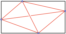
Figure 1. A maximal singularity-free rectangle $R$ defines a tetrahedron equipped with a map into $R$.

A singularity-free rectangle in $\widehat{X}$ is an embedded rectangle whose edges are leaf segments of the lifts of $\lambda^{\pm}$ and whose interior contains no singularities of $\widehat{X}$. If $R$ is a maximal singularity-free rectangle in $\widehat{X}$ then it contains exactly one singularity on the interior of each edge. The four singularities span a quadrilateral in $R$ which we can think of as the image of a tetrahedron by a projection map whose fibers are intervals, as pictured in Figure 1.

The tetrahedra of $\mathcal{N}$ are identified with all such tetrahedra, up to the action of $\pi_{1}(\mathring{X})$, where the restriction of $\Pi$ is exactly this projection to the rectangles, followed by $p$.

A $\tau$-edge in $\mathring{X}$ is the $\Pi$-image of an edge of $\tau$, or equivalently a saddle connection of $q$ whose lift to $\widetilde{\mathring{X}}$ spans a singularity-free rectangle. A $\tau$-edge in $X$ or $\overline{X}$ is the closure of a $\tau$-edge in $\mathring{X}$.

When $\phi\colon S\to S$ is a pseudo-Anosov homeomorphism, let $(X,q)$ denote $S$ endowed with a quadratic-differential $q$ whose foliations are the stable and unstable foliations of $\phi$. Then $\lambda^{\pm}$ have no saddle connections so we may construct $\mathcal{N}$, on which $\phi$ induces a simplicial homeomorphism $\Phi$ of $\mathcal{N}$, whose quotient $\mathring{M}_{\phi}$ is the mapping torus of $\phi|_{\mathring{S}}$. Equivalently, $\mathring{M}=\mathring{M}_{\phi}$ is obtained from the mapping torus $M_{\phi}$ by removing the singular orbits of its suspension flow, which we discuss next.

2.3. Fibered faces of the Thurston norm

Let $M$ be a finite-volume hyperbolic $3$-manifold. A fibration $\sigma\colon M\to S^{1}$ of $M$ over the circle comes with the following structure: there is a primitve integral cohomology class in $H^{1}(M;\mathbb{Z})$ represented by $\sigma_{*}\colon\pi_{1}M\to\mathbb{Z}$, which is the Poincaré dual of the fiber $F$. There is also a representation of $M$ as a quotient $\left(F\times\mathbb{R}\right)/\Phi$ where $\Phi(x,t)=(\phi(x),t-1)$ and where $\phi\colon F\to F$ is a pseudo-Anosov homeomorphism called the monodromy map. The map $\phi$ has stable and unstable (singular) measured foliations $\lambda^{+}$ and $\lambda^{-}$ on $F$. Finally there is the suspension flow inherited from the natural $\mathbb{R}$ action on $F\times\mathbb{R}$, and suspensions $\Lambda^{\pm}$ of $\lambda^{\pm}$ which are flow-invariant 2-dimensional foliations of $M$. Note that the deck transformation $\Phi$ translates in the opposite direction of the lifted flow. This is so that the first return map to the fiber $F$ equals $\phi$.

The fibrations of $M$ are organized by the Thurston norm $||\cdot||$ on $H^{1}(M;\mathbb{R})$ [Thu86] (see also [Fri79]). This norm has a polyhedral unit ball $B$ with the following properties:

1. Every cohomology class dual to a fiber is in the cone $\mathbb{R}_{+}\bf F$ over a top-dimensional open face $\bf F$ of $B$.

2. If $\mathbb{R}_{+}\bf F$ contains a cohomology class dual to a fiber then every primitive integral class in $\mathbb{R}_{+}\bf F$ is dual to a fiber. $\bf F$ is called a fibered face and its primitive integral classes are called fibered classes.

3. For a fibered class $\omega$ with associated fiber $F$, $||\omega||=-\chi(F)$.

In particular if $\dim H^{1}(M;\mathbb{R})\geq 2$ and $M$ is fibered then there are infinitely many fibrations, with fibers of arbitrarily large complexity. We will abuse terminology by saying that a fiber (rather than its Poincaré dual) is in $\mathbb{R}_{+}\bf F$.

The fibered faces also organize the suspension flows and the stable/unstable foliations: If $\bf F$ is a fibered face then there is a single flow $\psi$ and a single pair $\Lambda^{\pm}$ of foliations whose leaves are invariant by $\psi$, such that every fibration associated to $\mathbb{R}_{+}\bf F$ may be isotoped so that its suspension flow is $\psi$ up to a reparameterization, and the foliations $\lambda^{\pm}$ for the monodromy of its fiber $F$ are $\Lambda^{\pm}\cap F$. These results were proven by Fried [Fri82]; see also McMullen [McM00].

Finally, we note that the veering triangulation of $\mathring{M}$, like the flow itself, is an invariant of the fibered face containing the fiber $\mathring{S}$ (see [Ago12] or [MT17, Proposition 2.7]).

2.4. Subsurfaces, $q$–compatibility, and $\tau$–compatibility

We conclude this section by reviewing some essential constructions from [MT17] and direct the reader there for the full details. In short, the idea is that if $Y$ is a subsurface of $(X,q)$ with $d_{Y}(\lambda^{-},\lambda^{+})$ sufficiently large, then $Y$ has particularly nice forms; the first with respect to the $q$-metric, and the second with respect to $\tau$.

Let $Y\subset X$ be an essential compact subsurface, and let $X_{Y}=\widetilde{X}/\pi_{1}(Y)$ be the associated cover of $X$. We say a boundary component of $Y$ is puncture-parallel if it bounds a disk in $\overline{X}\smallsetminus Y$ that contains a single point of $\mathcal{P}$. We denote the corresponding subset of $\mathcal{P}$ by $\mathcal{P}_{Y}$ and refer to them as the punctures of $Y$. Let $\widetilde{\mathcal{P}}_{Y}$ denote the subset of punctures of $X_{Y}$ which are encircled by the boundary components of the lift of $Y$ to $X_{Y}$. In terms of the completed space $\overline{X}_{Y}$, $\widetilde{\mathcal{P}}_{Y}$ is exactly the set of completion points which have finite total angle. Let $\partial_{0}Y$ denote the union of the puncture-parallel components of $\partial Y$ and let $\partial^{\prime}Y$ denote the rest. Observe that the components of $\partial_{0}Y$ are in natural bijection with $\mathcal{P}_{Y}$ and set $Y^{\prime}=Y\smallsetminus\partial_{0}Y$.

Identifying $\widetilde{X}$ with $\mathbb{H}^{2}$, let $\Lambda\subset\partial\mathbb{H}^{2}$ be the limit set of $\pi_{1}(Y)$, $\Omega=\partial\mathbb{H}^{2}\smallsetminus\Lambda$, and $\widehat{\mathcal{P}}_{Y}\subset\Lambda$ the set of parabolic fixed points of $\pi_{1}(Y)$. Let $C(X_{Y})$ denote the compactification of $X_{Y}$ given by $(\mathbb{H}^{2}\cup\Omega\cup\widehat{\mathcal{P}}_{Y})/\pi_{1}(Y)$, adding a point for each puncture-parallel end of $X_{Y}$, and a circle for each of the other ends.

$q$-convex hulls

As above, identify $\widetilde{X}$ with $\mathbb{H}^{2}$. Let $\Lambda\subset\partial\mathbb{H}^{2}$ be a closed set and let ${\operatorname{CH}}(\Lambda)$ be the convex hull of $\Lambda$ in $\mathbb{H}^{2}$. Using the results of [MT17, Section 2.3], we define the $q$-convex hull ${\operatorname{CH}}_{q}(\Lambda)$ as follows.

Assume first that $\Lambda$ has at least 3 points. Each boundary geodesic $l$ of ${\operatorname{CH}}(\Lambda)$ has the same endpoints as a (biinfinite) $q$-geodesic $l_{q}$ in $\widehat{X}$ (we note that $l_{q}$ may meet $\partial\mathbb{H}^{2}$ at interior points). Further, $l_{q}$ is unique unless it is part of a parallel family of geodesics, making a Euclidean strip.

$\widehat{X}$ is divided by $l_{q}$ into two sides, and one of the sides, which we call $\mathcal{D}_{l}$, meets $\partial\mathbb{H}^{2}$ in a subset of the complement of $\Lambda$. The side $\mathcal{D}_{l}$ is either a disk or a string of disks attached along completion points. If $l_{q}$ is one of a parallel family of geodesics, we include this family in $\mathcal{D}_{l}$. After deleting from $\widehat{X}$ the interiors of $\mathcal{D}_{l}$ for all $l$ in $\partial{\operatorname{CH}}(\Lambda)$, we obtain ${\operatorname{CH}}_{q}(\Lambda)$, the $q$-convex hull.

If $\Lambda$ has 2 points then ${\operatorname{CH}}_{q}(\Lambda)$ is the closed Euclidean strip formed by the union of $q$-geodesics joining those two points.

Now fixing a subsurface $Y$ we can define a $q$-convex hull for the cover $X_{Y}$ by taking a quotient of the $q$-convex hull ${\operatorname{CH}}_{q}(\Lambda_{Y})$ of the limit set $\Lambda_{Y}$ of $\pi_{1}(Y)$. This quotient, which we will denote by ${\operatorname{CH}}_{q}(X_{Y})$, lies in the completion $\overline{X}_{Y}$. We remark that in general ${\operatorname{CH}}_{q}(X_{Y})$ may be a total mess, e.g. it may have empty interior.

$q$–compatibility

Let $\widehat{\iota}:Y\to X_{Y}$ be the lift of the inclusion map to the cover. We say that the subsurface $Y$ of $X$ is $q$-compatible if the interior of ${\operatorname{CH}}_{q}(\Lambda_{Y})$ is a disk. In this case, [MT17, Lemma 2.6] implies that $\widehat{\iota}\colon Y\to X_{Y}$ is homotopic to a map $\widehat{\iota}_{q}\colon Y\to\overline{X}_{Y}$ which restricts to a homeomorphism from $Y\smallsetminus\partial_{0}Y$ to

$$Y_{q}={\operatorname{CH}}_{q}(X_{Y})\smallsetminus\widetilde{\mathcal{P}}_{Y}$$ (2.4)

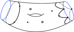
Figure 2. The image of a $q$-compatible subsurface $Y$ in $\overline{X}_{Y}$ under $\widehat{\iota}_{q}$. Open circles are points of $\widetilde{\mathcal{P}}_{Y}$ (corresponding to the image of $\partial_{0}Y$) and dots are singularities not contained in $\widetilde{\mathcal{P}}_{Y}$. The ideal boundary of $X_{Y}$ is in blue.

We recall that by [MT17, Lemma 5.1], if $Y$ is $q$-compatible, then

1. the projection $\iota_{q}\colon Y\to\overline{X}$ of $\widehat{\iota}_{q}$ to $\overline{X}$ is an embedding from $\mathrm{int}(Y)$ into $X$ which is homotopic to the inclusion, and

2. $\widehat{\iota}_{q}(\partial Y\smallsetminus\partial_{0}Y)$ does not pass through points of $\widetilde{\mathcal{P}}_{Y}$.

See Figure 2. The embedded image $\iota_{q}(\mathrm{int}(Y))$ is an open representative of $Y$ in $X$ and is denoted $\mathrm{int}_{q}(Y)$.

The following is our main tool for proving $q$-compatibility; it is [MT17, Proposition 5.2].

Proposition 2.4 ($q$-Compatibility).

Let $Y\subset X$ be an essential subsurface.

1. If $Y$ is nonannular and $d_{Y}(\lambda^{-},\lambda^{+})\geq 3$, then $Y$ is $q$-compatible.

2. If $Y$ is an annulus and $d_{Y}(\lambda^{-},\lambda^{+})\geq 4$, then $Y$ is $q$-compatible. In this case, $\mathrm{int}_{q}(Y)$ is a flat cylinder.

We remark that the constants in [MT17, Proposition 5.2] are slightly different since there $d_{Y}$ was defined to be the minimal distance between projections.

$\tau$–compatibility

Next we focus on compatibility with respect to the veering triangulation. Call a $q$-compatible subsurface $Y\subset X$ $\tau$-compatible if the map $\widehat{\iota}_{q}\colon Y\to\overline{X}_{Y}$ is homotopic rel $\partial_{0}Y$ to a map $\widehat{\iota}_{\tau}:Y\to\overline{X}_{Y}$ which is an embedding on $Y^{\prime}=Y\smallsetminus\partial_{0}Y$ such that

1. $\widehat{\iota}_{\tau}$ takes each component of $\partial^{\prime}Y=\partial Y\smallsetminus\partial_{0}Y$ to a simple curve in $\overline{X}_{Y}\smallsetminus\widetilde{\mathcal{P}}_{Y}$ composed of a union of $\tau$-edges and

2. the map $\iota_{\tau}\colon Y\to\overline{X}$ obtained by composing $\widehat{\iota}_{\tau}$ with $\overline{X}_{Y}\to\overline{X}$ restricts to an embedding from $\mathrm{int}(Y)$ into $X$.

When the subsurface $Y$ is $\tau$-compatible, we set

$$\partial_{\tau}Y\equiv\iota_{\tau}(\partial^{\prime}Y)$$ (2.5)

which is a collection of $\tau$-edges with disjoint interiors. We call $\partial_{\tau}Y$ the $\tau$–boundary of $Y$ and consider it as a $1$-complex of $\tau$-edges in $X$. (At times we will also think of $\partial_{\tau}Y$ as a collection of disjoint $\tau$-edges in the fully-punctured surface $\mathring{X}$.) Similar to the situation of a $q$-compatible subsurface, if $Y$ is $\tau$-compatible then one component of $X\smallsetminus\partial_{\tau}Y$ is an open subsurface isotopic to the interior of $Y$; this is the image $\iota_{\tau}(\mathrm{int}(Y))$ and is denoted $\mathrm{int}_{\tau}(Y)$. For future reference, we set $Y_{\tau}\subset X_{Y}$ to be the intersection of $X_{Y}$ with the image of $\widehat{\iota}_{\tau}$. By definition, the covering $X_{Y}\to X$ maps the interior of $Y_{\tau}$ homeomorphically onto $\mathrm{int}_{\tau}(Y)$.

The following result is Theorem 5.3 of [MT17].

Theorem 2.5 ($\tau$-Compatibility).

Let $Y\subset X$ be an essential subsurface.

1. If $Y$ is nonannular and $d_{Y}(\lambda^{-},\lambda^{+})\geq 3$, then $Y$ is $\tau$-compatible.

2. If $Y$ is an annulus and $d_{Y}(\lambda^{-},\lambda^{+})\geq 4$, then $Y$ is $\tau$-compatible.

The comment following Proposition 2.4 also applies here.

3. Veering triangulations and subsurfaces

Here we study the connection between sections of the bundle $\mathcal{N}\to\mathring{X}$ and projections to subsurfaces of $X$. In brief, we tailor the theory of subsurface projections to the veering structure. This is accomplished in Lemma 3.6 and Proposition 3.7.

3.1. Sections of the veering triangulation

A section of the veering triangulation $\tau$ in $\mathcal{N}$ is a simplicial embedding $s\colon(\mathring{X},\Delta)\to\mathcal{N}$ that is a section of the fibration $\Pi\colon\mathcal{N}\to\mathring{X}$. Here, $\Delta$ is an ideal triangulation of $\mathring{X}$, which by construction consists of $\tau$–edges. We will also refer to the image of $s$ in $\mathcal{N}$, which we often denote by $T$, as a section.

There is a bijective correspondence between sections of $\mathcal{N}$ and ideal triangulations of $\mathring{X}$ by $\tau$–edges. More generally, we use the notation $\Pi_{*}$ to denote the map that associates to any subcomplex of a section the corresponding union of $\tau$–simplices of $\mathring{X}$, and we use $\Pi^{*}$ to denote its inverse. In particular, if $K$ is a union of disjoint $\tau$–edges of $\mathring{X}$, $\Pi^{*}(K)$ is the subcomplex of $\mathcal{N}$ obtained by lifting its simplices to $\mathcal{N}$. Note that $T$ and $T^{\prime}$ differ by a tetrahedron move in $\mathcal{N}$ if and only if the ideal triangulations $\Pi_{*}(T)$ and $\Pi_{*}(T^{\prime})$ differ by a diagonal exchange. Here, an upward (downward) tetrahedron move on a section $T$ replaces two adjacent faces at the bottom (top) of a tetrahedron with the two adjacent top (bottom) faces.

Since the fibers of $\Pi\colon\mathcal{N}\to\mathring{X}$ give $\mathcal{N}$ an oriented foliation by lines and each of these lines meets each section exactly once, we have the following observation: For each $x\in\mathcal{N}$ and each section $T$ of $\mathcal{N}$, it makes sense to write $x\leq T$ or $x\geq T$ depending on whether $x$ lies weakly below or above $T$ along the orientation of the line through $x$. (Here, $x\leq T$ and $x\geq T$ imply that $x\in T$.) In fact, this ordering extends to each simplex of $\mathcal{N}$; we write $\sigma\leq T$ if $x\leq T$ for each $x\in\sigma$. Since we will use this fiberwise ordering for several (simplicial) constructions, it is important to note that it is consistent along simplices; that is, if $x\leq T$ and $\sigma$ is the smallest simplex containing $x$, then $\sigma\leq T$. Finally, if $K$ is a subcomplex of $\mathcal{N}$, then $K\leq T$ if for each simplex $\sigma$ of $K$, $\sigma\leq T$.

In [MT17, Section 2.1] we define a strict partial order among $\tau$-edges using their spanning rectangles: if $e$ crosses $f$ we say that $e>f$ if $e$ crosses the spanning rectangle of $f$ from top to bottom, and $f$ crosses the spanning rectangle of $e$ from left to right (i.e. if the slope of $e$ is greater than the slope of $f$). A priori, this partial order is defined in the universal cover $\widetilde{X}$, but it projects consistently to $\mathring{X}$ and so defines a partial order of $\tau$-edges there as well. See Figure 3.

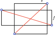
Figure 3. Two $\tau$-edges with $e>f$.

This definition is consistent with the ordering of the simplices $\Pi^{*}(e)$, $\Pi^{*}(f)$ in $\mathcal{N}$, and in particular

Lemma 3.1.

$K\leq T$ if and only if whenever an edge $e$ of $\Pi_{*}(T)$ crosses an edge $f$ of $\Pi_{*}(K)$, we have $f<e$.

Proof.

First, let $f$ be any $\tau$-edge in $\mathring{X}$ and let $\Delta$ be a triangulation of $\mathring{X}$ by $\tau$-edges. By [MT17, Lemma 3.4], if $e$ is an edge of $\Delta$ and $e>f$, then there is an edge of $\Delta$ crossing $f$ which is downward flippable, meaning that there is a diagonal exchange of $\Delta$ replacing it with an edge of smaller slope. (An analogous statement holds if $f>e$.) Such a diagonal exchange results in a triangulation $\Delta^{\prime}$ either containing $f$ or still containing an edge $e^{\prime}$ with $e^{\prime}>f$. After finitely many downward diagonal exchanges, we arrive at a triangulation by $\tau$-edges which contains the edge $f$. (See [MT17, Section 3] for details.) Translating this statement to $\mathcal{N}$, this means that starting with $\Pi^{*}(\Delta)$ there is a sequence of downward tetrahedron moves resulting in a section containing $\Pi^{*}(f)$. Hence, $\Pi^{*}(f)\leq\Pi^{*}(\Delta)$

This, together with the corresponding result for when $K\geq T$, implies the lemma. ∎

Given sections $T_{1}$ and $T_{2}$, we use $U(T_{1},T_{2})$ to denote the subcomplex of $\mathcal{N}$ between them. Formally, $U(T_{1},T_{2})$ is the subcomplex of $\mathcal{N}$ which is the union of all simplices $\sigma$ such that either $T_{1}\leq\sigma\leq T_{2}$ or $T_{2}\leq\sigma\leq T_{1}$.

It will be helpful to consider the lattice structure of sections. For sections $T_{1},T_{2}$, we denote their fiberwise maximum by $T_{1}\vee T_{2}$. If we name the oriented fiber containing $x$ by $l_{x}$, this is the subset $\{x\in\mathcal{N}:x=\max_{l}\{l_{x}\cap T_{1},l_{x}\cap T_{2}\}\}$, where the max is taken with respect to the ordering on each $l_{x}$.

Lemma 3.2.

$T_{1}\vee T_{2}$ is a section.

Proof.

Since the restriction of $\Pi$ to $T_{1}\vee T_{2}$ is a homeomorphism to $\mathring{X}$, it suffices to show that $T_{1}\vee T_{2}$ is a subcomplex of $\mathcal{N}$. Let $x\in T_{1}\vee T_{2}$ and suppose that $x$ is contained in $T_{1}$. Then $x\geq T_{2}$ and so if $\sigma$ is the minimal simplex of $T_{1}$ containing $x$, we see $\sigma\geq T_{2}$. Hence, $\sigma\subset T_{1}\vee T_{2}$ and we conclude that $T_{1}\vee T_{2}$ is indeed a section. ∎

We can define the minimum $T_{1}\wedge T_{2}$ of two sections similarly. With this terminology, it makes sense to say that $T_{1}\vee T_{2}$ is the top of $U(T_{1},T_{2})$. More precisely, $T_{1}\vee T_{2}\subset U(T_{1},T_{2})$ and for every simplex $\sigma\subset U(T_{1},T_{2})$, $\sigma\leq T_{1}\vee T_{2}$. Similarly, we say that $T_{1}\wedge T_{2}$ is the bottom of $U(T_{1},T_{2})$. Further, using our definitions we see that

$$U(T_{1},T_{2})=U(T_{1}\wedge T_{2},T_{1}\vee T_{2}).$$

Note that the part of $T_{1}$ that lies above $T_{2}$ is $T_{1}\cap(T_{1}\vee T_{2})$.

Sections through a subcomplex

Let $E\subset\mathring{X}$ be a union of disjoint $\tau$–edges and set $K=\Pi^{*}(E)$ to be the corresponding subcomplex of $\mathcal{N}$. (Our primary example will be $E=\partial_{\tau}Y$ for a $\tau$-compatible subsurface $Y$ of $X$. In this situation we think of $\partial_{\tau}Y$ as a collection of $\tau$-edges of $\mathring{X}$.) We define $T(E)=T(K)$ to be the set of sections of $\mathcal{N}$ which contain $K$ as a subcomplex. Similarly, we define $\Delta(E)=\Delta(K)$ as the set of ideal triangulations of $\mathring{X}$ by $\tau$–edges containing $E$. We recall the following two basic results from [MT17]. The first states simply that $T(E)$ is nonempty. It is [MT17, Lemma 3.2].

Lemma 3.3 (Extension lemma).

Suppose that $E$ is a collection of $\tau$-edges in $\mathring{X}$ with pairwise disjoint interiors. Then $T(E)$ is nonempty.

The second ([MT17, Proposition 3.3]) states that $T(K)$ is always connected by tetrahedron moves. This includes in particular the case of $T(\emptyset)$, the set of all sections.

Lemma 3.4 (Connectivity).

If $E$ is a collection of $\tau$-edges in $X$ with pairwise disjoint interiors, then $\Delta(E)$ is connected via diagonal exchanges. In terms of $\mathcal{N}$, for $K=\Pi^{*}(E)$, $T(K)$ is connected via tetrahedron moves.

Moreover, if $T_{1},T_{2}\in T(K)$ with $T_{1}\leq T_{2}$, then there is a sequence of upward tetrahedron moves from $T_{1}$ to $T_{2}$ through sections of $T(K)$.

As explained in [MT17, Corollary 3.6], whenever $E\neq\emptyset$, there is a well-defined top $T^{+}$ and bottom $T^{-}$ of $T(E)$. That is, $T^{+}\in T(E)$ and for any $T\in T(E)$, $T\leq T^{+}$.

$\phi$-sections. Suppose that $q$ is a quadratic differential associated to a pseudo-Anosov homeomorphism $\phi$. Recall that the deck transformation $\Phi$ of $\mathcal{N}$ is chosen to translate in the opposite direction of the flow.

Say that a section $T$ of the veering triangulation $\tau$ is a $\phi$–section if $\Phi(T)\leq T$. In other words, $T$ is a $\phi$–section if every $\tau$-edge of $\Pi_{*}(\Phi(T))=\phi(\Pi_{*}(T))$ which crosses a $\tau$-edge of $\Pi_{*}(T)$ does so with lesser slope. Note that if $T$ is a $\phi$–section, then $\Phi^{j}(T)\leq\Phi^{i}(T)$ for all $i\leq j$.

Agol’s original construction produces a veering triangulation from a sequence of diagonal exchanges through $\phi$-sections [Ago11, Proposition 4.2]. In fact, he proves

Lemma 3.5 (Agol).

There is a sweep-out of $\tau$ through $\phi$–sections. That is, there is a sequence $(T_{i})_{i\in\mathbb{Z}}$ of $\phi$–sections such that $T_{i+1}$ is obtained from $T_{i}$ by simultaneous upward tetrahedron moves.

3.2. Projections to $\tau$–compatible subsurfaces

In this section we define a variant of the subsurface projections $\pi_{Y}$ that is adapted to the simplicial structure of $\tau$. In the hyperbolic setting, $\pi_{Y}(\alpha)$ can be defined using the geodesic representatives of the surface $Y$ and the curve $\alpha$. In our setting we need to use the simplicial representative $Y_{\tau}$ of a $\tau$-compatible surface $Y$ and a collection of $\tau$-edges representing $\alpha$. The main result here will be Proposition 3.7, which shows, in a suitable setting, that the simplicial variant of the projection is uniformly close to the usual notion.

Recall first the notion of a proper graph $G$ in a surface from Section 2.1.3 and its image $\mathcal{A}_{S}(G)$ in the arc graph (Definition 2.3).

If $E$ is a collection of $\tau$–edges of $\mathring{X}$ with disjoint interiors, then its closure in $X$, $\mathrm{cl}_{X}(E)$, is a proper graph. This is the union of the corresponding saddle connections in $X$. In particular if $K$ is a subcomplex of a section then $E=\Pi_{*}(K^{(1)})$ is such a collection of $\tau$-edges and we make the notational abbreviation

$$\mathcal{A}_{X}(K)=\mathcal{A}_{X}(\mathrm{cl}_{X}(\Pi_{*}(K^{(1)}))).$$ (3.1)

Note that for any section $T$, we have (Corollary 2.3) $\mathrm{diam}(\mathcal{A}_{X}(T))\leq D$, where $D=15$.

Suppose now that $Y\subset X$ is a $\tau$–compatible nonannular subsurface and $G\subset X$ is a union of $\tau$–edges with disjoint interiors (i.e. a proper graph of $\tau$-edges). Then $\mathrm{int}_{\tau}(Y)\cap G$ is a proper graph in $\mathrm{int}_{\tau}(Y)$ and we set

$$\pi_{Y}^{\tau}(G)=\mathcal{A}_{Y}(\mathrm{int}_{\tau}(Y)\cap G).$$ (3.2)

Note that this could in general be empty, if $\mathrm{int}_{\tau}(Y)\cap G$ is not essential.

When $Y$ is a $\tau$-compatible annulus, $\mathrm{int}_{\tau}(Y)\cap G$ is a collection of disjoint arcs each of which is contained in the interior of a $\tau$-edge. Taking the preimages of these $\tau$-edges in $X_{Y}$, we obtain the projection $\pi_{Y}^{\tau}(G)$ by associating to each such $\tau$-edge $a$ that joins opposite sides of $\partial Y_{\tau}\subset X_{Y}$ the collection of complete $q$-geodesics $a^{*}$ in $X_{Y}$ that contain it. Each of these geodesics gives a well-defined arc of $\mathcal{A}(Y)=\mathcal{A}(X_{Y})$, and if here are no such $\tau$-edges, then the projection is empty.

In general, this notion of subsurface projection is easily extended to a subcomplex $K$ of a section of $\mathcal{N}$, in analogy with (3.1). We simply write:

$$\pi_{Y}^{\tau}(K)=\pi_{Y}^{\tau}(\mathrm{cl}_{X}(\Pi_{*}(K^{(1)}))).$$ (3.3)

Finally, we define the subsurface distance between subcomplexes $K_{1}$ and $K_{2}$ to be

$$d_{Y}(K_{1},K_{2})=d_{Y}(\pi^{\tau}_{Y}(K_{1}),\pi^{\tau}_{Y}(K_{2})).$$ (3.4)

The following lemma establishes some important technical properties of $\tau$-compatible subsurfaces. Key to the argument is the construction of $\mathrm{int}_{\tau}(Y)$ from $\mathrm{int}_{q}(Y)$ that appears in [MT17, Theorem 5.3] and is illustrated in Figure 4.

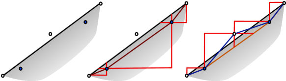
Figure 4. Left: $\mathrm{int}_{q}(Y)$ is shaded, contains the blue singularities, and its boundary contains the black saddle connection. Middle: the ‘inner t-hull construction’ isotopes the surface within itself; its new boundary consists of saddle connections (dark red) through the blue singularities. Right: $\mathrm{int}_{\tau}(Y)$, whose boundary consists of $\tau$-edges (blue), is then produced with the ‘outer t-hull construction.’

We remark that one difficulty in what follows is that the $\tau$-representative $\mathrm{int}_{\tau}(Y)$, unlike the $q$-representative $\mathrm{int}_{q}(Y)$, is not convex with respect to the $q$ metric.

Lemma 3.6.

Let $Y$ and $Z$ be $\tau$-compatible subsurfaces of $X$ and let $G\subset X$ be a proper graph of $\tau$-edges.

1. The diameter $\mathrm{diam}_{Y}(\pi_{Y}^{\tau}(G))$ is bounded by $D=15$. If $Y$ is an annulus, then $\mathrm{diam}_{Y}(\pi_{Y}^{\tau}(G))\leq 3$.

2. If $Y$ and $Z$ are disjoint then so are $\mathrm{int}_{\tau}(Y)$ and $\mathrm{int}_{\tau}(Z)$.

3. The subsurface $\mathrm{int}_{\tau}(Y)$ is in minimal position with the foliation $\lambda^{\pm}$. In particular, the arcs of $\mathrm{int}_{\tau}(Y)\cap\lambda^{\pm}$ agree with the arcs of $\pi_{Y}(\lambda^{\pm})$.

Proof.

The graph $G\cap\mathrm{int}_{\tau}(Y)$ has its vertices in $\mathrm{int}_{\tau}(Y)\cap\mathrm{sing}(q)$. By Gauss–Bonnet, $|\mathrm{int}_{\tau}(Y)\cap\mathrm{sing}(q)|\leq 2|\chi(Y)|$, and so $(1)$ follows from Corollary 2.3 when $Y$ is not an annulus.

If $Y$ is an annulus, then recall that $\mathrm{int}_{q}(Y)$ is a flat annulus and that $\mathrm{int}_{q}(Y)\subset\mathrm{int}_{\tau}(Y)$ since the process of going from the $q$-hull to the $\tau$-hull for annuli only pushes outward (c.f. [MT17, Remark 5.4]). Lifting to the annular cover $X_{Y}$, let $a,b$ be $\tau$-edge coming from $G$ that join opposite sides of $Y_{\tau}$. Then $a$ and $b$ are disjoint and any of their $q$-geodesic extensions $a^{*},b^{*}$ cross the maximal open flat annulus $\mathrm{int}_{q}(Y)$ of $X_{Y}$ in subsegments of $a,b$, respectively. Moreover, by a standard Gauss–Bonnet argument (e.g. [Raf05, Lemma 3.8]), any two $q$-geodesic segments intersect at most once in any component of $X_{Y}\smallsetminus\mathrm{int}_{q}(Y)$. Hence, $a^{*},b^{*}$ intersect at most twice and so $\mathrm{diam}_{Y}(\pi_{Y}^{\tau}(G))\leq 3$ when $Y$ is an annulus.

Items $(2)$ and $(3)$ follow exactly as in [MT17, Lemma 6.1]. As that lemma was proven only in the fully-punctured case, we note that in general for item $(2)$ one must perform the inner ${\mathbf{t}}$-hull construction (middle of Figure 4) as an intermediate step. However, since this pushes each surface within itself, it must preserve disjointness. For $(3)$, the isotopy from $\mathrm{int}_{q}(Y)$ to $\mathrm{int}_{\tau}(Y)$ pushes along the leaves of $\lambda^{+}$ (or $\lambda^{-}$). Hence, the leaves of $\lambda^{+}$ (or $\lambda^{-}$) are in minimal position with $\mathrm{int}_{\tau}(Y)$ since they are with $\mathrm{int}_{q}(Y)$, by the local CAT$(0)$ geometry. ∎

We note that it follows from Lemma 3.6.(3) (or directly from its proof) that if $\widetilde{\lambda}^{\pm}$ are the lifts of $\lambda^{\pm}$ to $\widetilde{X}$ and $C^{\tau}_{Y}$ is a component of the preimage of $\mathrm{int}_{\tau}(Y)$, then the intersection of $C^{\tau}_{Y}$ with each leaf of $\widetilde{\lambda}^{\pm}$ is connected.

The following proposition relates the projections defined here to the usual notion of subsurface projection.

Proposition 3.7.

Let $Y,Z$ be $\tau$–compatible subsurfaces of $X$ and suppose that $\pi_{Z}(\partial Y)\neq\emptyset$. Further assume that $d_{Y}(\lambda^{-},\lambda^{+})\geq 3$ (or if $Y$ is an annulus that $d_{Y}(\lambda^{-},\lambda^{+})\geq 6$). Then

$$\mathrm{diam}_{Z}\big{(}\pi_{Z}^{\tau}(\partial_{\tau}Y)\cup\pi_{Z}(\partial Y)\big{)}\leq 7.$$

As usual, let $X_{Z}$ denote the $Z$–cover of $X$. In this subsection, a core $Z^{\prime}$ of $X_{Z}$ is a submanifold with boundary which is a complementary component of simple curves and proper arcs such that $Z^{\prime}\to X_{Z}$ is a homotopy equivalence. This definition includes the usual convex core in the hyperbolic metric as well as $Z_{\tau}\subset X_{Z}$ (Section 2.4). In general, $\partial Z^{\prime}\subset X_{Z}$ is a collection of curves and arcs.

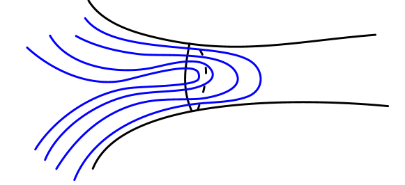
Figure 5. The curve/arc $\gamma$ (blue) is in $4$-position with respect to $\partial Z$, but not $3$–position. Note that the arcs of $\partial Z$ cobounding these bigons are nested.

Let $\gamma$ be any essential curve or proper arc in $X_{Z}$. Note that $\gamma$ may not be in minimal position with $\partial Z^{\prime}$, that is, there may be bigons between arcs of $\gamma$ and $\partial Z^{\prime}$. To handle this situation, we make the following definition: For some $k\geq 0$, we say that $\gamma$ is in $k$–position with respect to $\partial Z^{\prime}$ if $k$ is the largest integer such that a collection of $k$ nested subsegments of $\partial Z^{\prime}$ cobound bigons with subsegments of $\gamma$ whose interiors are contained in $X_{Z}\smallsetminus Z^{\prime}$. See Figure 5.

The point of this condition is the following lemma.

Lemma 3.8.

Suppose that $Z$ is a nonannular subsurface of $X$ and that $X_{Z}$ and $Z^{\prime}$ are as above. Let $\gamma$ be an essential curve or proper arc in $X_{Z}$ which is in $k$–position with respect to $\partial Z^{\prime}$, and let $y$ be an essential arc of $\gamma\cap Z^{\prime}$. Then

$$d_{Z}(y,\pi_{Z}(\gamma))\leq 2\log(2k)+2.$$

Proof.

To prove the lemma, we consider $y$ as an arc of $X_{Z}$ as follows: for each endpoint $p\in y\cap\partial Z^{\prime}$ append to $y$ a proper ray in $X_{Z}$ starting at $p$ which meets $Z^{\prime}$ only at $p$. Let $y^{*}$ denote the resulting essential arc of $X_{Z}$. (Under the implicit/canonical identification $\mathcal{A}(\mathrm{int}(Z^{\prime}))\cong\mathcal{A}(X_{Z})$, $y$ and $y^{*}$ are identified.) Now we claim that as isotopy classes of arcs in $X_{Z}$, $y^{*}$ and $\gamma$ have at most $2k$ essential intersections, thus proving the lemma.

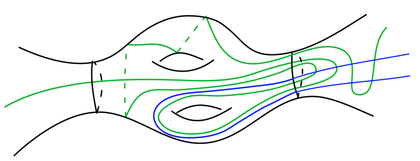
Figure 6. The arc $\gamma$ (green) is in $2$-position with $\partial Z$. The arc $y^{*}$ (blue) intersects $\gamma$ essentially no more than twice.

For this, first push $y^{*}$ slightly to one side of itself, so that $y^{*}$ and $\gamma$ are transverse. Then each point $p_{i}\in y^{*}\cap\partial Z^{\prime}$ ($i=1,2$) is contained in no more than $k$ nested subsegments of $\partial Z^{\prime}$ which cobound bigons $\mathcal{B}_{i}$ with $\gamma$, as in the definition of $k$-position. See Figure 6.

Since each component of $X_{Z}\smallsetminus\mathrm{int}(Z^{\prime})$ is a disk or annulus, it follows that there is an isotopy supported in $X_{Z}\smallsetminus\mathrm{int}(Z^{\prime}\cup\mathcal{B}_{1}\cup\mathcal{B}_{2})$ which removes all of the intersections between $\gamma$ and $y^{*}$ which are not contained in $\mathcal{B}_{1}\cup\mathcal{B}_{2}$. Hence, $\gamma$ and $y^{*}$ have at most $2k$ essential intersections. This completes the proof. ∎

Because $\mathrm{int}_{\tau}(Y)$ is an open subsurface representative of $Y$, it does not provide a good representative of $\partial Y$. So for the proof of Proposition 3.7 we do the following: Let $Y_{n}$ ($n\geq 1$) be the exhaustion of $\mathrm{int}_{\tau}(Y)$ by subsurface isotopic to $Y$ obtained by removing the open $\epsilon_{n}$–neighborhood of $\partial_{\tau}Y$. Here, $\epsilon_{n}\to 0$ as $n\to\infty$, and distance is taken with respect to the flat metric $q$. Note that by our definitions, each $\mathcal{A}(Y_{n})$ is naturally identified with $\mathcal{A}(Y)$. When $Y$ is not an annulus, will use the property that, through this identification, for any curve or arc $a$ in $X$, the collection of curves and arcs in $\mathcal{A}(Y)$ given by $a\cap Y_{n}$ eventually agrees with the collection given by $a\cap\mathrm{int}_{\tau}(Y)$.

Proof of Proposition 3.7.

First suppose that $Z$ is not an annulus.

As above, let $Y_{n}$ be the exhaustion of $\mathrm{int}_{\tau}(Y)$ introduced above. To keep notation simple, we set $Y=Y_{n}$ for $n$ sufficiently large (to be determined later). Note that by construction $\partial Y$ and $\partial_{\tau}Y$ are disjoint in $X$. Hence, if $\gamma$ is any essential component of the preimage of $\partial Y$ in $X_{Z}$, then $\gamma$ is disjoint from the preimage of $\partial_{\tau}Y$. Letting $y$ be any essential component of $\gamma\cap Z_{\tau}$, this shows that $d_{Z}(y,\pi_{Z}^{\tau}(\partial_{\tau}Y))\leq 1$. Hence, it suffices to bound the distance between $y$ and $\pi_{Z}(\gamma)$ in $\mathcal{A}(Z)$. This will follow from Lemma 3.8, once we show that $\gamma$ is in $2$–position with respect to $\partial Z_{\tau}$ in $X_{Z}$.

Suppose that this were not the case; that is, suppose that there is a point $p\in\partial Z_{\tau}$ which is contained in $3$ nested subsegments of $\partial Z_{\tau}$, each of which cobounds a bigon with a subarc of $\gamma$ contained in $X_{Z}\smallsetminus\mathrm{int}(Z_{\tau})$. We now lift this picture to $\widetilde{X}$ to produces a component $C^{\tau}_{Z}$ of the preimage of $Z_{\tau}$ in $\widetilde{X}$, a point $\widetilde{p}\in\partial C^{\tau}_{Z}$, and arcs $\widetilde{\gamma}_{1},\widetilde{\gamma}_{2},\widetilde{\gamma}_{3}$ in the preimage of $\gamma$ that cobound bigons with nested subsegments of $\partial C^{\tau}_{Z}$ containing $\widetilde{p}$. (The arcs are ordered so that $\widetilde{\gamma}_{1}$ is innermost, i.e, closest to $\widetilde{p}$, and $\widetilde{\gamma}_{3}$ is outermost.) Let $B$ be the bigon cobounded by a subarc of $\partial C^{\tau}_{Z}$ and $\widetilde{\gamma}_{3}$.

Since these arcs are components of preimages of $\partial Y$, we can use them to produce a component $C_{Y}$ of the preimage of $Y$ in $\widetilde{X}$ such that

1. some component of $\partial C_{Y}$ contains $\widetilde{\gamma}_{1}$ or $\widetilde{\gamma}_{2}$ , and

2. $C_{Y}\cap B$ contains a component which is a disk whose sides alternate between subarcs of $\partial C_{Y}$ and subarcs of $\partial C^{\tau}_{Z}$.

For simplicity, we assume that $\widetilde{\gamma}_{1}$ is contained in the component of $\partial C_{Y}$ in item $(1)$ and denote the other component of $\partial C_{Y}\cap B$ that appears in item $(2)$ by $\widetilde{\eta}$. (It may be that $\widetilde{\eta}=\widetilde{\gamma}_{2}$.) See Figure 7.

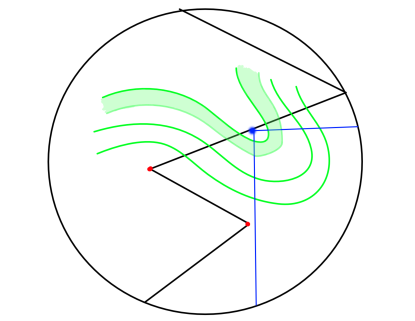
Figure 7. The component $C_{Y}$ (green) and its intersection with $l^{\pm}$ (blue). The intersection of the black zig-zag arc with $\widetilde{X}$ give components of $\partial C^{\tau}_{Z}$.

Now since the leaves of $\lambda^{\pm}$ are in minimal position with respect to $Z_{\tau}$ (Lemma 3.6 and the comment that follows), the intersection of each leaf of $\widetilde{\lambda}^{\pm}$ (the lifts of $\lambda^{\pm}$ to $\widetilde{X}$) with $C^{\tau}_{Z}$ is connected. Hence, we may choose subrays $l^{\pm}$ in $\widetilde{\lambda}^{\pm}$ which are based at $\widetilde{p}$ and are disjoint from $\mathrm{int}(C^{\tau}_{Z})$. By condition $(2)$ above, each of $l^{\pm}$ must pass first through $\widetilde{\gamma}_{1}$ and then through $\widetilde{\eta}$. Moreover, each of $l^{\pm}\cap C_{Y}$ is an arc joining distinct components of $\partial C_{Y}$, once $n$ is sufficiently large, again by Lemma 3.6 this time applied to $Y$.

If $Y$ is also nonannular, then we conclude that the two leaf segments $\lambda^{\pm}\cap C_{Y}$ project to give homotopic components of $\lambda^{+}\cap Y$ and $\lambda^{-}\cap Y$. Once $n$ is sufficiently large, these gives homotopic components of $\lambda^{+}\cap\mathrm{int}_{\tau}(Y)$ and $\lambda^{-}\cap\mathrm{int}_{\tau}(Y)$ and by Lemma 3.6 we see that $d_{Y}(\lambda^{+},\lambda^{-})\leq 2$. This contradiction shows that $\gamma$ is in $2$-position with $\partial Z_{\tau}$ and completes the proof when neither $Y$ nor $Z$ are annuli.

If $Y$ is an annulus, then as remarked above $\mathrm{int}_{q}(Y)$ is a flat annulus and $\mathrm{int}_{q}(Y)\subset\mathrm{int}_{\tau}(Y)$. The argument above produces rays $l^{\pm}$ such that $l^{\pm}\cap C_{Y}$ are leaf segments of $\widetilde{\lambda}^{\pm}$. We claim that these segments project to disjoint arcs of $Y$. Otherwise, there is a deck transformation $g$ that stabilizes $C_{Y}$ such that $(g\cdot l^{-}\cap l^{+})\cap C_{Y}$ is nonempty. In this case, we have $g\cdot B\cap B\neq\emptyset$ (where $B$ is the bigon from above) and so $g\cdot C^{\tau}_{Z}\cap C^{\tau}_{Z}\neq\emptyset$. Since, $Z$ is $\tau$-compatible, this implies that $g$ stabilizes $C^{\tau}_{Z}$ and contradicts our assumption that $Y$ and $Z$ overlap.

Hence, we conclude that $l^{\pm}\cap C_{Y}$ project to disjoint leaf segments in $Y\subset\mathrm{int}_{\tau}(Y)\subset X_{Y}$. For $n$ large as above, these leaves do not intersect again before exiting $\mathrm{int}_{\tau}(Y)$ in $X_{Y}$. Since leaves of $\lambda^{\pm}$ intersect at most once outside the maximal open flat annulus $\mathrm{int}(Y_{q})\subset X_{Y}$, this produces representatives of $\pi_{Y}(\lambda^{-})$ and $\pi_{Y}(\lambda^{+})$ intersecting at most twice. Hence, $d_{Y}(\lambda^{+},\lambda^{-})\leq 5$ giving the same contradiction as before.

It remains to establish the proposition when $Z$ is an annulus. Since $\pi_{Z}(\partial Y)\neq\emptyset$, there is a $\tau$-edge in the lift of $\partial_{\tau}Y$ to $X_{Z}$ that joins boundary components of $Z_{\tau}$ on opposite sides of the core curve of $X_{Z}$. Fix any such $\tau$-edge $a$. Since $\mathrm{int}_{q}(Z)\subset\mathrm{int}_{\tau}(Z)$, $a$ crosses $\mathrm{int}_{q}(Z)\subset X_{Z}$ and has its endpoints in $X_{Z}\smallsetminus\mathrm{int}_{q}(Z)$. Recall the definition $a^{*}\in\pi_{Z}^{\tau}(\partial_{\tau}Y)$ from the discussion following Equation 3.2.

Let $\gamma$ be any essential component of the lift of $\partial Y$ to $X_{Z}$ and let $\gamma_{q}$ be its geodesic representative in the $q$-metric. As before, the preimage of $\partial Y$ in $X_{Z}$ can be made disjoint from $\gamma_{q}$ since $Y$ is $q$-compatible. Since $\gamma_{q}$ is a $q$-geodesic, its intersection with $\mathrm{int}_{q}(Z)\subset X_{Z}$ is contained in a single saddle connection $b$. Moreover, because $Y$ is $\tau$-compatible, any saddle connection of $\partial_{q}Y\subset X$ intersects any $\tau$-edge of $\partial_{\tau}Y\subset X$ at most once in its interior (see e.g. [MT17, Theorem 5.3]) and so $a$ and $b$ intersect at most once. If $a^{*}$ is any extension of $a$ to a complete $q$-geodesic in $X_{Y}$, then we have by the same Gauss–Bonnet argument as for the proof of Lemma 3.6 that $\gamma_{q}$ intersects $a^{*}$ at most three times. We conclude that

$$\mathrm{diam}_{Z}\big{(}\pi_{Z}^{\tau}(\partial_{\tau}Y)\cup\pi_{Z}(\partial Y)\big{)}\leq 2+d_{Z}(a^{*},\gamma_{q})\leq 6,$$

and the proof is complete. ∎

4. From immersions to covers

When defining the subsurface projection $\pi_{Y}$ for a subsurface $Y\subset S$ we consider preimages of curves in the cover $S_{Y}$ associated to $Y$. Of course, the same operation can be done for any cover of $S$ corresponding to a finitely generated subgroup of $\pi_{1}(S)$. The main theorem of this section (Theorem 4.1, which is Theorem 1.3 in the introduction) gives a concrete explanation for why these more general projections do not capture additional information. This will be an essential ingredient for the proof of Theorem 7.1.

First, for a finitely generated subgroup $\Gamma<\pi_{1}(S)$, let $S_{\Gamma}\to S$ be the corresponding cover. If $Y\subset S_{\Gamma}$ is a compact core the covering map restricted to $Y$ is an immersion and we say that $Y\to S$ corresponds to $\Gamma<\pi_{1}(S)$. Lifting to the cover induces a (partially defined) map of curve and arc graphs which we denote $\pi_{Y}\colon\mathcal{A}(S)\to\mathcal{A}(Y)$, and we define $d_{Y}(\alpha,\beta)$ and $\mathrm{diam}_{Y}$ accordingly. Note that these constructions depend on $\Gamma$ and not on the choice of $Y$, and that $\pi_{Y}$ agrees with the usual subsurface projection when $Y\subset S$.

The goal of this section is the following theorem, which may be of independent interest:

Theorem 4.1 (Immersion to cover).

There is a uniform constant $M\leq 38$ satisfying the following: Let $S$ be a surface and let $Y\to S$ be an immersion corresponding to a finitely-generated $\Gamma<\pi_{1}(S)$. Then either $\mathrm{diam}_{Y}(\mathcal{A}(S))\leq M$, or $Y\to S$ is homotopic to a finite cover $Y\to W$ for $W$ a subsurface of $S$.

Theorem 4.1 will follow as a corollary of the following statement:

Theorem 4.2.

Let $Y\to S$ be an immersion corresponding to $\Gamma<\pi_{1}(S)$, and let $\lambda^{\pm}$ be a transverse pair of foliations without saddle connections. If $d_{Y}(\lambda^{-},\lambda^{+})\geq 37$, then $Y\to S$ is homotopic to a finite cover $Y\to W$ for $W$ a subsurface of $S$.

Let $q$ be a quadratic differential whose horizontal and vertical foliations are $\lambda^{\pm}$, and let $X$ denote $S$ endowed with $q$. For curve or arc $\delta$, denote its horizontal length with respect to $q$ by $h_{q}(\delta)$ and its vertical length with respect to $q$ by $v_{q}(\delta)$. For a homotopy class we let $h_{q}$ and $v_{q}$ denote the minima over all representatives. Recall that a multicurve $\gamma$ is balanced at $q$ if $h_{q}(\gamma)=v_{q}(\gamma)$. For the quadratic differential $q$ and a multicurve $\gamma$, there is always some time $t\in\mathbb{R}$ such that $\gamma$ is balanced at $q_{t}$, where $q_{t}$ is the image of $q$ under the Teichmüller flow for time $t$.

We let $X_{Y}=X_{\Gamma}$ denote the associated cover and recall from Section 2.4, the definition of the $q$-hull $Y_{q}\subset X_{Y}$. If $d_{Y}(\lambda^{-},\lambda^{+})\geq 5$ then $Y_{q}$ is embedded in $X_{Y}$, by which we mean the map $\hat{\iota}_{q}$ is an embedding on $Y\smallsetminus\partial_{0}Y$ (Proposition 2.4). In the language of the previous section $Y_{q}$ is a core of $X_{Y}$ and $\partial Y_{q}\subset X_{Y}$ is a collection of locally geodesic curves and proper arcs (of finite $q$-length).

If $\alpha,\beta$ are curves or properly embedded arcs in $X$, then we let

$$j_{Y}(\alpha,\beta)$$

denote the minimum, over all components $a$ of $\pi_{Y}(\alpha)$ and $b$ of $\pi_{Y}(\beta)$, of the number of intersection points of $a$ and $b$. We may also use the same notation if $\alpha,\beta$ are laminations in $S$, or essential curves or properly embedded arcs in $Y$. The following inequality comes essentially from [Raf05]:

Lemma 4.3.

Suppose $Y_{q}$ is embedded in the cover $X_{Y}$ and $\partial Y$ is balanced with respect to $q$. Then for any essential curve or arc $\delta$ in $Y_{q}$, we have

$$4\cdot\ell_{q}(\delta)\geq j_{Y}(\lambda,\delta)\cdot\ell_{q}(\partial Y),$$

for $\lambda$ equal to either $\lambda^{+}$ or $\lambda^{-}$.

Proof.

We show the inequality for $\lambda^{+}$. First recall that $Y_{q}$ contains a union of maximal vertical strips $S_{1},\ldots,S_{n}$ with disjoint, singularity–free interiors having the property that $h_{q}(\partial Y)=2\sum_{i}h_{q}(S_{i})$. Here, $h_{q}(S_{i})$ denotes the width of the strip $S_{i}$. For details of this construction, see [Raf05, Section 5]. If $\delta$ is an essential curve or arc of $Y_{q}$, then $\delta$ crosses each strip $S_{i}$ at least $j_{Y}(\delta,\lambda^{+})$ times since each strip is foliated by segments of $\lambda^{+}$. Hence

$$h_{q}(\delta)\geq\sum_{i}h_{q}(S_{i})\cdot j_{Y}(\delta,\lambda^{+})=\frac{1}{2}h_{q}(\partial Y)\cdot j_{Y}(\delta,\lambda^{+}).$$

Since $\partial Y$ is balanced, $h_{q}(\partial Y)=v_{q}(\partial Y)$ and so $\ell_{q}(\partial Y)\leq 2h_{q}(\partial Y)$. We conclude

$$\ell_{q}(\delta)\geq h_{q}(\delta)\geq\frac{1}{4}\ell_{q}(\partial Y)\cdot j_{Y}(\delta,\lambda^{+})$$

as required. ∎

We now proceed with the proof of Theorem 4.2.

Proof.

We may suppose that $d_{Y}(\lambda^{-},\lambda^{+})\geq 5$ so that $Y_{q}$ is embedded in $X_{Y}$. If $Y$ is an annulus, then $\mathrm{int}(Y_{q})\subset X_{Y}$ is a flat annulus which must cover a flat annulus in $X$. So we now suppose that $Y$ is not an annulus. We may further assume, applying the Teichmüller flow to $q$ if necessary, that $\partial Y_{q}$ is balanced.

Let $P$ be either $S^{1}$ or $\mathbb{R}$. If $\gamma\colon P\to X_{Y}$ is a parameterization of a boundary component of $Y_{q}$ (see Figure 2), then we say that a re-elevation of $\gamma$ is any lift to $X_{Y}$ of $\mathbb{R}\to P\overset{\gamma}{\to}X_{Y}\overset{p}{\to}X$, where $\mathbb{R}\to P$ is the universal cover, and we say that the re-elevation is essential if it meets $Y_{q}$ essentially. From nonpositive curvature of the metric, a re-elevation is essential if and only if it meets $\mathrm{int}(Y_{q})$.

We note that with this terminology, $Y\to X$ covers a subsurface of $X$ if and only if there are no essential re-elevations of components of $\partial Y_{q}$, since in this case $p^{-1}(p(\partial Y_{q}))\cap Y_{q}=\partial Y_{q}$ (see [MT17, Lemma 6.6]). Thus our goal now is to prove that if $d_{Y}(\lambda^{-},\lambda^{+})$ is sufficiently large, independent of $Y$ and $X$, then there are no essential re-elevations of $\partial Y_{q}$.

Let $g\colon\mathbb{R}\to X_{Y}$ be a re-elevation of $\gamma$, let $(a,b)\subset\mathbb{R}$ be a component of $g^{-1}(\mathrm{int}_{q}Y)$, and let $\widetilde{\gamma}$ denote the restriction of $g$ to $[a,b]$. This is a geodesic path (possibly with self-intersection) with endpoints in $\partial Y_{q}$, and if $g$ is essential then $\widetilde{\gamma}$ may be chosen to be essential.

We now look for a restriction of $\widetilde{\gamma}$ to an essential simple arc or curve. Let $d\in[a,b]$ be the supremum over $t\in[a,b]$ for which $\widetilde{\gamma}|_{[a,t]}$ is an embedding.

Case 1:

$d<b$. Then there exists $c\in[a,d)$ such that $\widetilde{\gamma}(d)=\widetilde{\gamma}(c)$. Thus $x=\widetilde{\gamma}|_{[c,d]}$ is an embedded loop.

Case 1a:

$x$ is an essential loop, which we name $\sigma$.

In the case where $P=S^{1}$, divide $\mathbb{R}$ into fundamental domains for the covering map $\mathbb{R}\to S^{1}$, so that $c$ is a boundary point of a fundamental domain, and let $l\geq 0$ be the number of full fundamental domains contained in $[c,d]$. When $P=\mathbb{R}$, set $l=0$. Hence, as $\gamma$ is a component of $\partial_{q}Y$,

$$\ell_{q}(\sigma)\leq\ell_{q}(\widetilde{\gamma}|_{[c,d]})\leq(l+1)\cdot\ell_{q}(\partial_{q}Y).$$

By Lemma 4.3,

$$j_{Y}(\lambda^{\pm},\sigma)\cdot\ell_{q}(\partial Y)\leq 4\cdot\ell_{q}(\sigma)\leq 4(l+1)\cdot\ell_{q}(\partial Y)$$

and so $j_{Y}(\lambda^{\pm},\sigma)\leq 4(l+1)$.

The Gauss–Bonnet theorem for the Euclidean cone metric on $Y_{q}$ implies that the number of singularities in the interior of $Y_{q}$ is no more than $2|\chi(Y)|$ and since $\widetilde{\gamma}|_{[c,d]}$ is an embedded loop, it visits each of these singularities of $Y_{q}$ at most once. As $\widetilde{\gamma}|_{[c,d]}$ contains at least $l$ singularities interior to $Y_{q}$, we obtain $l\leq 2|\chi(Y)|$. Combining this with the inequality arrived at above, we conclude that

$$j_{Y}(\lambda^{\pm},\sigma)\leq 4(2\cdot|\chi(Y)|+1).$$ (4.1)

We now invoke Lemma 2.2 (and in particular eq. 2.1) to conclude that $d_{Y}(\lambda^{\pm},\sigma)\leq 15$. Hence, $d_{Y}(\lambda^{-},\lambda^{+})\leq 30$ as required.

Case 1b:

If $x=\widetilde{\gamma}|_{[c,d]}$ is inessential, it still cannot be null-homotopic since $g$ is a geodesic path, so it must be peripheral. That is, either $x$ bounds a punctured disk in $Y_{q}$ or $x$ cobounds an annulus $A$ with a boundary component $u$ of $Y_{q}$. We claim that in the latter case the endpoint $\widetilde{\gamma}(a)$ does not lie on $u$.

Figure 8. When $\widetilde{\gamma}$ meets itself but glances off the annulus $A$, we obtain a geodesic loop homotopic to the boundary component $u$.

Suppose otherwise. Then there are two possibilities. If $\widetilde{\gamma}|_{[d,d+\epsilon)}$ does not enter $A$, then $x$ is a $q$-geodesic loop: at $\widetilde{\gamma}(c)$ it subtends an angle of at least $\pi$ inside $A$, and at $\widetilde{\gamma}(d)$ it subtends an angle of at least $\pi$ outside $A$. (See Figure 8). But this is a contradiction – $x$ cannot be a geodesic representative of $u$ and not equal to $u$.

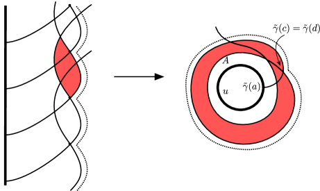
Figure 9. On the right is the annulus $A$ formed when $\gamma$ crosses itself at its first intersection point. Its thickening $A^{\prime}$ is indicated by the dotted circle. At left is the universal cover of $A^{\prime}$ where one can see the bigon between translates of the lift of $\widetilde{\gamma}$.

If $\widetilde{\gamma}|_{[d,d+\epsilon)}$ enters $A$ for small $\epsilon$, then we claim there is an immersed $q$-geodesic bigon cobounded by arcs of $\widetilde{\gamma}$, which contradicts nonpositive curvature. Indeed, thicken $A$ slightly to an annulus $A^{\prime}$ and let $t>d$ be the smallest value for which $\widetilde{\gamma}(t)$ meets $\partial A^{\prime}\smallsetminus u$. Consider the lifts of $\widetilde{\gamma}|_{[a,t]}$ to the universal cover $\widetilde{A}^{\prime}$ of $A^{\prime}$. This cover is an infinite strip, and the lifts form a $\mathbb{Z}$-periodic sequence of arcs connecting the two boundary components. One may order the lifts by their endpoints on (either) boundary component, and then we see that, since each lift crosses the lift above it at a preimage of $\widetilde{\gamma}(d)$, two consecutive lifts must intersect at least twice. This produces an immersed bigon downstairs, and our contradiction (see Figure 9).

Figure 10. $\sigma$ is formed from the self-intersection of $\widetilde{\gamma}$. The inner circle represents $u$ or the puncture.

We conclude that the concatenation $\sigma$ of $\widetilde{\gamma}|_{[a,d]}$ followed by $\widetilde{\gamma}|_{[a,c]}$ traversed in the opposite direction is an essential arc of $Y_{q}$ which is homotopic to an embedded arc (Figure 10). Moreover, since $x$ is embedded, $\sigma$ meets no singularity interior to $Y_{q}$ more than twice. Hence, if we let $l\geq 0$ be the number of fundamental domains in $[a,d]$, defined exactly as above, then $\ell_{q}(\sigma)\leq 2\ell_{q}(\widetilde{\gamma}|_{[a,d]})\leq 2(l+1)\cdot\ell_{q}(\partial Y)$. Using the same reasoning as in the previous case, we conclude that $j_{Y}(\lambda^{\pm},\sigma)\leq 8(l+1)$. Using the fact that $\sigma$ meets no singularity of $Y_{q}$ more than twice, we have $l\leq 4|\chi(Y)|$ and hence

$$j_{Y}(\lambda^{\pm},\sigma)\leq 8(4\cdot|\chi(Y)|+1).$$

This time we apply eq. 2.2 to conclude that $d_{Y}(\lambda^{\pm}\sigma)\leq 18$ and so $d_{Y}(\lambda^{-},\lambda^{+})\leq 36$.

Case 2:

$d=b$. This final case is handled just like Case 1a, except that $\sigma=\widetilde{\gamma}$ is an essential arc with embedded interior, rather than an essential loop. ∎

Theorem 4.1 now follows as a corollary:

Proof.

Suppose that $Y$ does not cover a subsurface of $S$. Let $\alpha,\beta$ be two curves with nontrivial projection to $Y$ and let $(\lambda^{\alpha}_{n})_{n\geq 0}$ and $(\lambda^{\beta}_{n})_{n\geq 0}$ be any sequences of filling laminations such that $\alpha$ is contained the Hausdorff limit of $\lambda^{\alpha}_{n}$ and $\beta$ is contained in the Hausdorff limit of $\lambda^{\beta}_{n}$. For example, if $f\colon S\to S$ is any pseudo-Anosov homeomorphism then we can take the stable and unstable laminations of $T^{n}_{\alpha}\circ f\circ T^{n}_{\beta}$ which is pseudo-Anosov for all but finitely many $n\in\mathbb{Z}$. Here $T_{\gamma}$ denotes the Dehn twist about the curve $\gamma$.

Now let $q_{n}=q(\lambda^{\alpha}_{n},\lambda^{\beta}_{n})$ be the holomorphic quadratic differential whose vertical and horizontal foliations are determined by $\lambda^{\alpha}_{n}$ and $\lambda^{\beta}_{n}$, respectively. By Theorem 4.2, then $d_{Y}(\lambda^{\alpha}_{n},\lambda^{\beta}_{n})\leq 36$ for each $n\in\mathbb{Z}$. However, for large enough $n\geq 0$, $\pi_{Y}(\alpha)\subset\pi_{Y}(\lambda^{\alpha}_{n})$ and $\pi_{Y}(\beta)\subset\pi_{Y}(\lambda_{n}^{\beta})$ and we conclude that $d_{Y}(\alpha,\beta)\leq 36$. Since $\alpha$ and $\beta$ were arbitrary curves with nontrivial projection to $Y$, we conclude that $\mathrm{diam}_{Y}(\mathcal{A}(S))\leq 38$. ∎

5. Uniform bounds in the veering triangulation

In this section we produce two estimates relating sections of the veering triangulation to subsurface projections in the original surface $X$. In Proposition 5.1, we show that for a $\tau$-compatible subsurface $Y$ of $X$, the $\pi_{Y}^{\tau}$-projections of the top and bottom sections of $T(\partial_{\tau}Y)$ are near the projections of $\lambda^{+}$ and $\lambda^{-}$, respectively, to $\mathcal{A}(Y)$. In Lemma 5.2, we show that if sections $T_{1}$ and $T_{2}$ have sufficiently far apart $\pi_{Y}^{\tau}$-projections to $\mathcal{A}(Y)$, then they must differ by at least $|\chi(Y)|$ tetrahedron moves in the veering triangulation. Both estimates will be important ingredients in the proof of Theorem 6.1.

5.1. Top/bottom of the pocket and distance to $\lambda^{\pm}$

Let $Y\subset X$ be a $\tau$-compatible subsurface as in Section 2.4. Since $\partial_{\tau}Y$ is a collection of edges of $\tau$ with disjoint interiors in $X$, Lemma 3.3 gives that $T(\partial_{\tau}Y)\neq\emptyset$. Let $T^{\pm}\in T(\partial_{\tau}Y)$ denote the top and bottom sections containing $\partial_{\tau}Y$.

The following proposition is analogous to [MT17, Proposition 6.2] in the fully punctured setting. However, more work is needed here to relate the projection of $T^{+}$ to the projection of $\lambda^{+}$ in the curve and arc graph of $Y$.

Proposition 5.1 (Compatibility with $\tau$ and distance to $\lambda^{\pm}$).

Let $T^{\pm}$ be the top and bottom sections in $T(\partial_{\tau}Y)$. For any section $Q\geq T^{+}$, $d_{Y}(Q,\lambda^{+})\leq D+1$ and for any $Q\leq T^{-}$, $d_{Y}(Q,\lambda^{-})\leq D+1$.

Recall that $d_{Y}(Q,\lambda^{-})$ means $d_{Y}(\pi_{Y}^{\tau}(Q),\pi_{Y}(\lambda^{-}))$.

Proof.

We begin by remarking that if $\mathrm{int}_{\tau}(Y)$ contains no singularities of $q$ other than punctures (i.e. if $\mathcal{P}_{Y}=\mathrm{sing}(q)\cap\mathrm{int}_{\tau}(Y)$ in $\overline{X}$), then the argument from [MT17, Proposition 6.2] carries through and gives a better constant. This includes the situation where $Y$ is an annulus.

In the general (nonannular) case, we show that there is an embedded edge path $p$ in $\Pi_{*}(Q)=\Delta_{Q}$ which projects to an essential arc of $\mathrm{int}_{\tau}(Y)$ and is isotopic to a properly embedded arc of $\mathrm{int}_{\tau}(Y)\cap\lambda^{+}$. Together with Lemma 3.6, this shows that

$$d_{Y}(Q,\lambda^{+})=d_{Y}(\pi_{Y}^{\tau}(Q),\lambda^{+})=\mathrm{diam}_{Y}(\pi_{Y}^{\tau}(Q))+\mathrm{diam}_{Y}(\lambda^{+})\leq D+1$$

as required (the proof for $\lambda^{-}$ is identical).

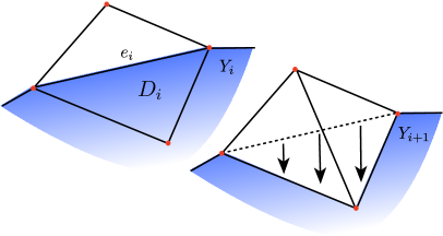
Figure 11. The first step: The upward diagonal exchange along the boundary and removing the triangle $D_{i}$. Vertices lie in $\mathrm{sing}(q)\cup\mathcal{P}$.

Let $T_{0},T_{1},T_{2},\ldots$ be any sequence of sections through upward tetrahedron moves starting with $T_{0}=T^{+}$ such that $Q=T_{j}$ for some $j\geq 0$ (Lemma 3.4), and let $\Delta_{i}=\Pi_{*}(T_{i})$ be the corresponding $\tau$-triangulations of $X$. Note that $\Delta_{i+1}$ is obtained from $\Delta_{i}$ by a single diagonal exchange.

Since $T_{0}\in T(\partial_{\tau}Y)$, $\Delta_{0}$ contains a subcomplex $Y_{0}$ which triangulates the image of $Y_{\tau}$ under the covering $X_{Y}\to X$. We inductively construct a sequence of subcomplexes $Y_{0}\supset Y_{1}\supset\ldots\supset Y_{n+1}$ of $\Delta_{0}\subset X$ satisfying certain conditions. For this, we say that each $Y_{i}$ comes with a boundary $\partial_{\tau}Y_{i}$, which is defined inductively below, and we set $\mathrm{int}_{\tau}(Y_{i})=Y_{i}\smallsetminus\partial_{\tau}Y_{i}$. For $Y_{0}$, $\partial_{\tau}Y_{0}=\partial_{\tau}Y$ so that $\mathrm{int}_{\tau}(Y)=Y_{0}\smallsetminus\partial_{\tau}Y_{0}$ is isotopic to $Y$.

To construct $Y_{i+1}$ from $Y_{i}$ observe that the upward exchange from $\Delta_{i}$ to $\Delta_{i+1}$ either occurs along an edge not meeting $Y_{i}$, in which case we set $Y_{i+1}=Y_{i}$, or it must occur along an edge $e_{i}$ of $\partial_{\tau}Y_{i}$. Otherwise, the edge $e_{i}$ lies in the interior of $Y_{i}\subset Y_{0}$ where it is wider (with respect to $q$) than the other edges in its two adjacent triangles. Hence, the same must be true in the triangulation $\Delta_{0}$, and we see that $\Pi^{*}(e_{i})$ is upward flippable in $T^{+}$. This gives a section $T^{\prime}\in T(\partial_{\tau}Y)$ with $T^{+}<T^{\prime}$, contradicting the definition of $T^{+}$.

Let $Q_{i}$ be the quadrilateral in $\Delta_{i}$ whose diagonal is $e_{i}$. Writing $Q_{i}$ as two triangles adjacent along $e_{i}$, at least one of them, call it $D_{i}$, is contained in $Y_{i}$, as in Figure 11. If $D_{i}$ is the only triangle in $Y_{i}$, set $Y_{i+1}=Y_{i}\smallsetminus(\mathrm{int}(D_{i})\cup e_{i})$ and $\partial_{\tau}Y_{i+1}=(\partial_{\tau}Y_{i}\cup\partial D_{i})\smallsetminus e_{i}$.

If the other triangle $D^{\prime}_{i}$ of $Q_{i}$ is also in $Y_{i}$, set $Y_{i+1}=Y_{i}\smallsetminus\mathrm{int}(Q_{i})$ and $\partial_{\tau}Y_{i+1}=\partial_{\tau}Y_{i}\cup\partial Q_{i}\smallsetminus e_{i}$.

Let $v_{i}$ be the vertex of $D_{i}$ opposite $e_{i}$ (and $v^{\prime}_{i}$ the vertex of $D^{\prime}_{i}$ opposite $e_{i}$ if we are in the second case). If $v_{i}$ (or $v^{\prime}_{i}$) is contained in $\partial_{\tau}Y_{i}\cup\mathcal{P}$, or $v_{i}=v^{\prime}_{i}$, then we set $n=i$, so that $Y_{n+1}$ is the last step of the construction.

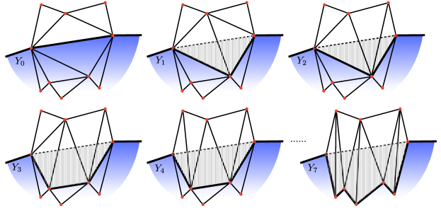
Figure 12. An example sequence of $Y_{i}$ (indicated in blue). A component $K$ of $\mathrm{int}_{\tau}(Y_{0})\smallsetminus Y_{i}$ is indicated with its $\lambda^{+}$ foliation in grey. $\sigma_{K}$, dotted, is the edge $e_{0}$.

The construction has the following properties for $i\leq n+1$:

1. $Y_{i}$ is a subcomplex of each of $\Delta_{0},\Delta_{1},\ldots,\Delta_{i}$. Moreover, the diagonal exchange from $\Delta_{i-1}$ to $\Delta_{i}$ replaces an edge $e_{i-1}$ in either $\partial_{\tau}Y_{i-1}$ or in the complement of $Y_{i-1}$.

2. Each component $K$ of $\mathrm{int}_{\tau}(Y_{0})\smallsetminus Y_{i}$ is a disk foliated by leaves of $\lambda^{+}$. Moreover, $\partial K$ is composed of two arcs $p_{K}$ and $\sigma_{K}$, where $\sigma_{K}$ is a $\tau$-edge in $\partial_{\tau}Y$ and $p_{K}$ is a path in $\partial_{\tau}Y_{i}$, and each leaf of the foliation of $K$ meets both $p_{K}$ and $\sigma_{K}$ at its endpoints.

3. For each component $K$ of $\mathrm{int}_{\tau}(Y_{0})\smallsetminus Y_{i}$ and each interior vertex $v$ of $p_{K}$, there is at least one edge $e$ of $\Delta_{i}$ entering $K$ from $v$, and every such edge crosses $\sigma_{K}$ from top to bottom, so that $e>\sigma_{K}$.

First note that $Y_{0}$ satisfies the properties for $i=0$ and that property $(1)$ holds for all $i\geq 0$ by construction.

Assume property (2) holds for $i\leq n$ and let us prove it for $i+1$. Let $D_{i}$ be the disk removed to obtain $Y_{i+1}$, and let $p_{D_{i}}$ be the other two sides of $\partial D_{i}$.

First suppose $e_{i}$ is in $\partial_{\tau}Y_{0}$ (which in particular holds for $i=0$). The two edges in $p_{D_{i}}$ cannot be in the boundary of any other component $K^{\prime}$ of $\mathrm{int}_{\tau}(Y_{0})\smallsetminus Y_{i}$, because then for some $j<i$ there would have been a $D_{j}$ whose third vertex $v_{j}$ was either a puncture or on $\partial_{\tau}Y_{0}$, which implies $j>n$. Thus $D_{i}$ itself is a component of $\mathrm{int}_{\tau}(Y_{0})\smallsetminus Y_{i+1}$, and (2) evidently holds, with $\sigma_{D_{i}}=e_{i}$.

Now if $e_{i}$ is not in $\partial_{\tau}Y_{0}$, it must lie in $p_{K}$ for some component $K$ of $\mathrm{int}_{\tau}(Y_{0})\smallsetminus Y_{i}$. We have again that $p_{D_{i}}$ cannot share edges with any other component of $\mathrm{int}_{\tau}(Y_{0})\smallsetminus Y_{i}$, and so we obtain a component $K^{\prime}$ of $\mathrm{int}_{\tau}(Y_{0})\smallsetminus Y_{i+1}$ by adjoining $D_{i}\smallsetminus p_{D_{i}}$ to $K$. The boundary path $p_{K^{\prime}}$ is obtained from $p_{K}$ by replacing $e_{i}$ by $p_{D_{i}}$, and the $\lambda^{+}$ foliation of $K$ extends across $e_{i}$ to $K^{\prime}$. The edge $\sigma_{K^{\prime}}$ is just $\sigma_{K}$.

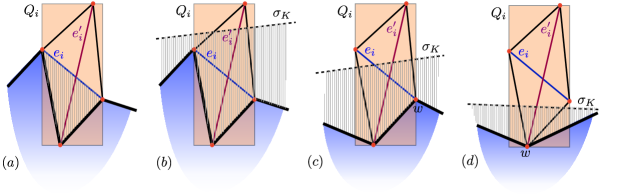
Figure 13. The proof of property (3)

Now we consider property (3). Breaking up into cases as in the proof of (2), consider first the case that $e_{i}$ is in $\partial_{\tau}Y_{0}$ (Figure 13(a)). Let $Q_{i}$ be the quadrilateral defining the move $\Delta_{i}\to\Delta_{i+1}$. Then the new edge $e^{\prime}_{i}$ is the other diagonal of $Q_{i}$ and must cross $e_{i}$. This shows that (3) holds for the new component $K=\mathrm{int}(D_{i})$ of $\mathrm{int}_{\tau}(Y_{0})\smallsetminus Y_{i+1}$.

If $e_{i}$ is in $p_{K}$ for some component $K$ of $\mathrm{int}_{\tau}(Y_{0})\smallsetminus Y_{i}$, consider $Q_{i}$ again (Figure 13(b)) and let $D^{\prime}_{i}$ be the complementary triangle to $D_{i}$ in $Q_{i}$. The two complementary edges to $e_{i}$ in $\partial D^{\prime}_{i}$ must, by inductively applying (3), cross $\sigma_{K}$. It follows that the new edge $e^{\prime}_{i}$ also crosses $\sigma_{K}$, thus proving (3) for $i+1$. Here, we are using the general fact that if an edge of a $\tau$-triangle crosses $\sigma$ from top to bottom, then so does the tallest edge of that triangle.

Finally suppose $e_{i}$ is outside of $Y_{i}$. If $Q_{i}$ is not adjacent to $Y_{i}$ at all then nothing changes and (3) continues to hold. If $Q_{i}$ shares a vertex $w$ with $p_{K}$ for some component $K$ of $\mathrm{int}_{\tau}(Y_{0})\smallsetminus Y_{i}$, we have a configuration like Figure 13(c) or (d). In (c), $w$ is on $e_{i}$. The new edge $e^{\prime}_{i}$, which connects to another vertex on $p_{K}$, must therefore also cross $\sigma_{K}$ (by transitivity of $<$). Moreover $w$ is still adjacent to one of the boundary edges of $Q_{i}$ which also passes through $\sigma_{K}$. Thus (3) is preserved at all vertices of $p_{K}$. In (d), $w$ is the vertex meeting $e^{\prime}_{i}$ and again we must have $e^{\prime}_{i}$ crossing $\sigma_{K}$. This concludes the proof of properties (1-3).

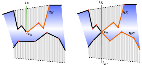
Figure 14. Two examples of $Y_{n+1}$ and the corresponding $\lambda^{+}$ arcs and $\Delta_{i}$ arcs. In the first case the point $v_{n}$ is a puncture so only one leaf $l_{K}$ and path $q_{K}$ is needed. In the second case $v_{n}$ lies on the boundary of two components of $\mathrm{int}_{\tau}(Y_{0})\smallsetminus Y_{n+1}$.

The sequence terminates with the diagonal exchange from $\Delta_{n}$ to $\Delta_{n+1}$ along an edge $e_{n}$ whose associated triangle $D_{n}$ has its opposite vertex $v_{n}$ in either $\mathcal{P}$ or the boundary of $Y_{n}$. There are either one or two components $K$ of $\mathrm{int}_{\tau}(Y_{0})\smallsetminus Y_{n+1}$ whose boundary path $p_{K}$ contains $v_{n}$. Examples of these two cases are shown in Figure 14.

For each such component $K$, let $l_{K}$ be the leaf of $\lambda^{+}$ adjacent to $v_{n}$ and exiting $K$ through $\sigma_{K}\subset\partial_{\tau}Y_{0}$, as in property (2). Let $q_{K}$ be a path along $p_{K}$ from $v_{n}$ to one of the endpoints of $p_{K}$. When there is only one component $K$, let $l=l_{K}$ and $q=q_{K}$. If there are two components $K,K^{\prime}$, let $l=l_{K}\cup l_{K^{\prime}}$ and $q=q_{K}\cup q_{K^{\prime}}$.

By Lemma 3.6, $l$ is an embedded essential arc of $\mathrm{int}_{\tau}Y$, and $q$ and $l$ define the same element of $\mathcal{A}(Y)$.

Recall that $\Pi_{*}(Q)=\Delta_{j}$. If $j\leq n+1$ we know that $Y_{n+1}$ is a subcomplex of $\Delta_{j}$ by (1), and hence we obtain a bound

$$d_{Y}(\Delta_{j},\lambda^{+})\leq D+1.$$

If $j>n+1$ we must consider what happens after further transitions. By (3), for each component $K$ of $\mathrm{int}_{\tau}(Y_{0})\smallsetminus Y_{n+1}$ adjacent to $v_{n}$, there is an edge $f_{n+1}$ of $\Delta_{n+1}$ adjacent to $v_{n}$, and passing through $K$ and exiting through $\sigma_{K}$. In particular the defining rectangle $R_{n+1}$ of $f_{n+1}$ passes through the rectangle of $\sigma_{K}$ from top to bottom. We claim that there is such an $f_{i}$ and $R_{i}$ for each $i\geq n+1$.

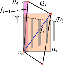
Figure 15. For $i>n$ we always find an edge in $\Delta_{i}$ starting at $v_{n}$ and exiting $K$ through $\sigma_{K}$.

If this holds for $i$, and the move $\Delta_{i}\to\Delta_{i+1}$ does not replace $f_{i}$ then we can let $R_{i+1}=R_{i}$ and $f_{i+1}=f_{i}$. If $f_{i}$ is replaced, there is a quadrilateral $Q_{i}$ in $\Delta_{i}$ of which $f_{i}$ is a diagonal, and one of the two edges of $\partial Q_{i}$ adjacent to $v_{n}$ must also cross the $\sigma_{K}$ rectangle from top to bottom. (See Figure 15).

Therefore, we can use these edges of $\Delta_{j}$ (either one or two depending on the number of components $K$ adjacent to $v_{n}$) to give an essential path in $\Delta_{j}$ which gives the same element of $\mathcal{A}(Y)$ as the leaf path $l$. We conclude again that

$$d_{Y}(\Delta_{j},\lambda^{+})\leq D+1$$

which completes the proof. ∎

5.2. Sweeping (slowly) through pockets

The following lemma states that in order to move a definite distance in the curve graph of $Y\subset X$ a certain number of edges, linear in the complexity of $Y$, need to be flipped. It will needed for the proof of Theorem 6.1.

Lemma 5.2 (Complexity slows progress).

Suppose that $T_{1},T_{2}\in T(\partial_{\tau}Y)$ are connected by no more than $|\chi(Y)|$ diagonal exchanges through sections of $T(\partial_{\tau}Y)$. Then $d_{Y}(T_{1},T_{2})\leq 2D$.

Proof.

We begin with the following claim:

Claim 1.

Let $\overline{Y}$ be a compact surface containing a finite (possibly empty) set $\mathcal{P}_{Y}\subset\mathrm{int}(\overline{Y})$, let $Y=\overline{Y}\smallsetminus\mathcal{P}_{Y}$, and assume that $\chi(Y)\leq-1$. Let $\overline{\Delta}$ be a triangulation of $\overline{Y}$ whose vertex set contains $\mathcal{P}_{Y}$ and consider the properly embedded graph $\Delta=\overline{\Delta}\smallsetminus\mathcal{P}_{Y}\subset Y$. If $E$ is a collection of nonboundary edges of $\Delta$ with $|E|\leq|\chi(Y)|$, there is $c\in\mathcal{A}(Y)$ that is nearly simple in $\Delta$ and traverses no edge of $E$.

Recall from Section 2.1.3 that $c$ is nearly simple in $\Delta$ if it is properly homotopic to path or curve in $\Delta$ that visits no vertex more than twice. Note that the conclusion of the claim is equivalent to the statement that the proper graph $\Delta^{(1)}\smallsetminus\mathrm{int}(E)$ is essential in $Y$.

Applying the claim to $\mathrm{int}_{\tau}(Y)$ gives $c\in\mathcal{A}(Y)$ which is nearly simple in the graph $\mathrm{cl}_{X}(\Pi_{*}((T_{1}\cap T_{2})^{(1)}))$. Hence, $d_{Y}(T_{1},T_{2})\leq 2D$.

Now it suffices to prove the claim:

Proof of claim.

First, we blow up the punctures $\mathcal{P}_{Y}$ to boundary components. That is, each $v\in\mathcal{P}_{Y}$ is replaced with a subdivided circle $S_{v}$ containing a vertex for each edge adjacent to $v$. Continue to call the resulting surface $Y$ and note that $\Delta$ induces a natural cell structure on $Y$, which we continue to denote by $\Delta$, made up of $n$-gons with $n\leq 6$. Obviously, $\chi(Y)$ is unchanged.

Considering $E$ as a possibly disconnected subgraph of $\Delta$, let $E^{\prime}$ be the edges of $E$ remaining after removing the components of $E$ which are contractible in $Y$ and do not meet $\partial Y$. Hence, every component of $Y\smallsetminus E^{\prime}$ is $\pi_{1}$–injective. We first claim that some component of $Y\smallsetminus E^{\prime}$ is neither a disk nor a boundary parallel annulus. Letting $G=E^{\prime}\cup\partial Y$, we have $\chi(Y)=\chi(Y\smallsetminus G)+\chi(G)$ since $Y\smallsetminus G$ is adjoined to $G$ along circles. Now $\chi(G)=\chi(\partial Y)+v-e=v-e$, where $v$ is the number of vertices in $E^{\prime}\smallsetminus\partial Y$ and $e=|E^{\prime}|$. If $Y\smallsetminus E^{\prime}$ consists of only $d\geq 0$ disks and $a\geq 0$ annuli then we have $\chi(Y\smallsetminus G)=\chi(Y\smallsetminus E^{\prime})=d$, and so $\chi(Y)=d+v-e$. Since an annulus must have a vertex of $E^{\prime}\smallsetminus\partial Y$ in its boundary, we note that if $d=0$ then $v>0$, and hence $d+v\geq 1$. We thus have $\chi(Y)\geq 1-|E^{\prime}|$, and so $|\chi(Y)|\leq|E^{\prime}|-1\leq|E|-1$, a contradiction.

Now let $U^{\prime}$ be some component of $Y\smallsetminus E^{\prime}$ which is neither a disc nor a boundary parallel annulus. Hence, there is an essential simple closed curve $\gamma^{\prime}$ of $Y$ contained in $U^{\prime}$. As $U=U^{\prime}\smallsetminus E$ has a component corresponding to $U^{\prime}$ minus a collection of disks, $\gamma^{\prime}$ is homotopic to a simple curve $\gamma$ in $U$. Let $c$ be a cell of $\Delta$ which $\gamma$ crosses. Since $c$ is a blown-up triangle, the edges that $\gamma$ crosses, which are in the complement of $E$, are connected along either vertices of $c$ or arcs of $\partial Y$ (which are also not in $E$). Thus $\gamma$ can be deformed to a curve in $\Delta$ that does not traverse the edges of $E$. This shows that the proper graph $\Delta^{(1)}\smallsetminus\mathrm{int}(E)$ is essential in $Y$ and the claim follows. ∎

This completes the proof of Lemma 5.2. ∎

6. Uniform bounds in a fibered face

In this section we prove the first main theorem of the paper. For a surface $Y$ recall that $|\chi^{\prime}(Y)|=\max\{|\chi(Y)|,1\}$.

Theorem 6.1 (Bounding projections for $M$).

Let $M$ be a hyperbolic fibered $3$-manifold with fibered face $\bf F$. Then for any fiber $S$ contained in $\mathbb{R}_{+}\bf F$ and any subsurface $Y$ of $S$

$$|\chi^{\prime}(Y)|\cdot(d_{Y}(\lambda^{-},\lambda^{+})-16D)\leq 2D\>|\bf F|,$$

where $|\bf F|$ is the number of tetrahedra of the veering triangulation associated to $\bf F$.

The proof of Theorem 6.1 requires the construction of an embedded subcomplex of $(\mathring{M},\tau)$ corresponding to $Y$ whose size is roughly $|\chi^{\prime}(Y)|\cdot d_{Y}(\lambda^{-},\lambda^{+})$.

6.1. Pockets and the approach from the fully-punctured case

Let us assume from now on that $d_{Y}(\lambda^{-},\lambda^{+})$ is sufficiently large that, by Theorem 2.5, $Y$ is $\tau$-compatible. We first describe an approach directly extending the argument from [MT17], and explain where it runs into trouble.

Recall from Section 3.1 the definition of $T(\partial_{\tau}Y)$, and its top and bottom sections $T^{+}$ and $T^{-}$. For any two sections $T_{1},T_{2}\in T(\partial_{\tau}Y)$ we have the region $U(T_{1},T_{2})$ in $\mathcal{N}$ between them. The closure of the open subsurface $\mathrm{int}_{\tau}(Y)$ in $X$ is the subspace $\mathcal{R}_{Y}$ which is the image of $Y_{\tau}\subset X_{Y}$ under the covering map $X_{Y}\to X$. Using this we further define

$$U_{Y}(T_{1},T_{2})=U(T_{1},T_{2})\cap\Pi^{-1}(\mathcal{R}_{Y})$$ (6.1)

to be the region between $T_{1}$ and $T_{2}$ that lies above $Y$. Note that $U_{Y}(T_{1},T_{2})$ is a subcomplex of $\mathcal{N}$. We sometimes call this the pinched pocket for $Y$ (between $T_{1}$ and $T_{2}$). We let

$$U_{Y}=U_{Y}(T^{-},T^{+})$$ (6.2)

denote the maximal pocket for $Y$.

By Proposition 5.1, $d_{Y}(T^{-},T^{+})$ is close to $d_{Y}(\lambda^{-},\lambda^{+})$. Thus when these are sufficiently large, by Lemma 5.2 we obtain a lower bound on the number of transitions between $T^{-}$ and $T^{+}$ in $\mathcal{N}$ that project to $\mathcal{R}_{Y}$, and in particular a lower bound on the number of tetrahedra in $U_{Y}$. If $U_{Y}$ were to embed in $\mathring{M}$ (equivalently if $U_{Y}$ were disjoint from all its translates by $\Phi$), this would give us what we need. It is not in general true, so instead we must restrict to a suitable sub-region of $U_{Y}$.

In the fully-punctured case, we can use the fact that, since every edge of $\tau$ represents an element of $\mathcal{A}(S)$, any intersection between $U_{Y}$ and $\Phi^{k}(U_{Y})$ would project to a non-empty $\pi_{Y}(\phi^{k}(\partial Y))$. Lemma 2.1 implies that, for $k>0$, whenever $\pi_{Y}(\phi^{k}(\partial Y))$ is non-empty it is close to $\pi_{Y}(\lambda^{-})$. Now by restricting $U_{Y}$ to a subcomplex $V_{Y}$ whose top and bottom surfaces are sufficiently far in $\mathcal{A}(Y)$ from $\lambda^{+}$ and $\lambda^{-}$, and applying this argument to $V_{Y}$, we see that $V_{Y}$ cannot meet $\Phi^{k}(V_{Y})$ at all.

In the general situation, since some singularities of $q$ are not punctures, not every collection of $\tau$-edges is essential and we are faced with the possibility that $U_{Y}$ and $\Phi^{k}(U_{Y})$ can intersect in large but homotopically inessential subcomplexes whose location is hard to control. This is the main difficulty.

6.2. Isolation via $\phi$-sections

We begin, therefore, with the following construction. Let $T_{0}$ denote a $\phi$-section (Section 3.1), so that $\phi^{k}(T_{0})\leq T_{0}$ for $k>0$. Define

$$N=N_{Y}=\min\{i>0:\phi^{i}(Y)\text{ overlaps }Y\}.$$ (6.3)

Now consider the (possibly empty) region

$$R(T_{0})=\mathrm{int}(U(\Phi^{N}(T_{0}),T_{0}))\cap\mathrm{int}(U_{Y}).$$ (6.4)

It easily satisfies the embedding property:

Proposition 6.2.

The restriction of the covering map $\mathcal{N}\to\ring{M}$ to $R(T_{0})$ is an embedding.

Proof.

We must show that $\Phi^{i}(R(T_{0}))$ is disjoint from $R(T_{0})$ for all $i>0$ (the case for $i<0$ immediately follows). For $i\geq N$ this is taken care of by the first term of the intersection since $T_{0}$ was chosen to be a $\phi$–section.

For $0<i<N$, we have that $\mathrm{int}_{\tau}(Y)$ and $\mathrm{int}_{\tau}(\phi^{i}(Y))$ are disjoint since the surfaces have no essential intersection, using Lemma 3.6. Therefore the interiors of $U_{Y}$ and $\Phi^{i}(U_{Y})$ are disjoint as well. ∎

What remains now is to choose $T_{0}$ so that a lower bound on $d_{Y}(\lambda^{-},\lambda^{+})$ implies a lower bound on the number of tetrahedra in $R(T_{0})$. That is, we want to view $R(T_{0})$ as the interior of a “pocket” between two sections, whose projections to $\mathcal{A}(Y)$ are close to $\lambda^{\pm}$. For this we will need to describe $R(T_{0})$ from a different point of view.

6.3. $Y$-projections of sections

For any section $T$ of $\mathcal{N}$, there is a corresponding section $T^{Y}\in T(\partial_{\tau}Y)$ obtained by pushing $T$ below $T^{+}$ and above $T^{-}$. More formally,

$$T^{Y}=T^{+}\wedge(T^{-}\vee T)=T^{-}\vee(T^{+}\wedge T).$$

To see what this does it is helpful to consider it along the fibers of $\Pi$ which we recall are oriented lines. For any $[a,b]\subset\mathbb{R}$, the map $x\mapsto b\wedge(a\vee x)$ is simply retraction of $\mathbb{R}$ to $[a,b]$, and is equal to $x\mapsto a\vee(b\wedge x)$.

Now we can use this projection to extend the notation $U_{Y}(T_{1},T_{2})$ (defined in (6.1)) to sections which are not necessarily in $T(\partial_{\tau}Y)$ by setting

$$\widehat{U}_{Y}(T_{1},T_{2})=U_{Y}(T_{1}^{Y},T_{2}^{Y})\subset U_{Y}.$$ (6.5)

This construction is related to the region $R(T_{0})$ defined in (6.4) by the following lemma:

Lemma 6.3.

$$\mathrm{int}(\widehat{U}_{Y}(T_{1},T_{2}))=\mathrm{int}(U(T_{1},T_{2}))\cap\mathrm{int}(U_{Y}).$$ (6.6)

Proof.

First consider what happens in each $\Pi$-fiber, which is just a statement about projections in $\mathbb{R}$: If $J=[s,t]$ is an interval in $\mathbb{R}$ we have, as above, the retraction $\pi_{J}(u)=s\vee(t\wedge u)$, and for any other interval $I$ we immediately find

$$\mathrm{int}(\pi_{J}(I))=\mathrm{int}(I)\cap\mathrm{int}(J).$$ (6.7)

To apply this to our situation note first that both the left and right hand sides of the equality (6.6) are contained in $\Pi^{-1}(\mathrm{int}_{\tau}(Y))$. This is because $U_{Y}$ is in $\Pi^{-1}(\mathcal{R}_{Y})$ and in $U(T^{-},T^{+})$, which means that for each $x\in\mathcal{R}_{Y}\smallsetminus\mathrm{int}_{\tau}(Y)=\partial_{\tau}Y$, $U_{Y}\cap\Pi^{-1}(x)$ is a single point, and hence not in the interior.

Now since $\Pi$ is a fibration, for any two sections $T,T^{\prime}$ and region $Z$ of the form $U(T,T^{\prime})\cap\Pi^{-1}(\Omega)$ where $\Omega$ is open, we have

$$\mathrm{int}(Z)\cap\Pi^{-1}(x)=\mathrm{int}(Z\cap\Pi^{-1}(x)).$$

For $x\in\mathrm{int}_{\tau}(Y)$, applying this to the left hand side of (6.6) we see that

$$\mathrm{int}(\widehat{U}_{Y}(T_{1},T_{2}))\cap\Pi^{-1}(x)=\mathrm{int}(\widehat{U}_{Y}(T_{1},T_{2})\cap\Pi^{-1}(x)).$$

On the right hand side, we obtain

$$\mathrm{int}(U(T_{1},T_{2}))\cap\Pi^{-1}(x)=\mathrm{int}(U(T_{1},T_{2})\cap\Pi^{-1}(x))$$

and

$$\mathrm{int}(U_{Y})\cap\Pi^{-1}(x)=\mathrm{int}(U_{Y}\cap\Pi^{-1}(x)).$$

This reduces the equality to a fiberwise equality, where it follows from (6.7). ∎

6.4. Relation between $T^{Y}$ and $\pi_{Y}$

A crucial point now is to show that the operation $T\to T^{Y}$ does not alter the projection to $\mathcal{A}(Y)$ by too much.

Proposition 6.4.

For all sections $T$ of $\mathcal{N}$, $d_{Y}(T,T^{Y})\leq 4D$.

Here $d_{Y}(T,T^{Y})$ is meant in the sense of (3.4).

Proof.

Write $T$ as a union of three subcomplexes, $T=K_{+}\cup K_{0}\cup K_{-}$, where

$$K_{0} =T\cap U(T^{-},T^{+}),$$

$$K_{+} =T\cap(T\vee T^{+}),$$

$$K_{-} =T\cap(T\wedge T^{-}).$$

See Figure 16. Since $T^{+},T^{-}\in T(\partial_{\tau}Y)$, $\Pi_{*}(K_{0})$ is a subcomplex of $\tau$-edges in $X$ that do not cross $\partial_{\tau}Y$.

Figure 16. The section $T$, its intersection with $U(T^{-},T^{+})$, and the decomposition $T=K_{+}\cup K_{0}\cup K_{-}$.

Lemma 6.5.

If $\pi_{Y}^{\tau}(K_{+})$ and $\pi_{Y}^{\tau}(K_{-})$ are empty then $\Pi_{*}(K_{0})$ contains a punctured spine for $Y$.

A punctured spine for $Y$ is a subspace which is a retract of $Y$ minus a union of disjoint disks. In other words, the conclusion of Lemma 6.5 implies that every essential curve in $Y$ is homotopic into $\Pi_{*}(K_{0})$. In particular, $\pi_{Y}^{\tau}(K_{0})$ is nonempty and so is every $\pi_{Z}^{\tau}(K_{0})$ for $Z$ a $\tau$-compatible subsurface that overlaps with $Y$.

Proof.

The statement that $\pi_{Y}^{\tau}(K_{+})$ is empty means that, after projecting $K_{+}$ by $\Pi$ into $X$ and intersecting with $\mathrm{int}_{\tau}(Y)$, we obtain components which are inessential subcomplexes, meaning they do not contain any essential curves or proper arcs. (When $Y$ is an annulus, this means that no $\tau$-edge from $K_{+}$ joins opposite sides of the open annulus $\mathrm{int}_{\tau}(Y)$.)

Now $K_{+}\smallsetminus K_{0}$ and $K_{-}\smallsetminus K_{0}$ are open in $T$ and disjoint, so their projections to $X$ intersect $\mathrm{int}_{\tau}(Y)$ in a collection of disjoint open sets each of which is inessential in the above sense. It follows that the complement of these open sets, which is $\Pi(K_{0})\cap\mathrm{int}_{\tau}(Y)$, intersects every essential curve and proper arc in $\mathrm{int}_{\tau}(Y)$. Hence it contains a punctured spine. ∎

If $T\cap U_{Y}$ projects to an essential subcomplex of $Y_{\tau}$, then the proposition follows since $T$ and $T^{Y}$ both contain $T\cap U_{Y}$.

If $T\cap U_{Y}$ is inessential then, by Lemma 6.5, at least one of $\pi_{Y}^{\tau}(K_{\pm})$ is nonempty. Suppose $\pi_{Y}^{\tau}(K_{+})$ is nonempty.

Since $K_{+}=T\cap(T\vee T^{+})$, we immediately have

$$d_{Y}(T,T\vee T^{+})\leq D.$$

Since $T^{+}\leq T\vee T^{+}$, Proposition 5.1 tells us that

$$d_{Y}(T\vee T^{+},\lambda^{+})\leq D.$$

Thus

$$d_{Y}(T,\lambda^{+})\leq 2D.$$

Now note that $T^{Y}\cap T^{+}$ is equal to the part of $T^{+}$ lying below $T$, hence its $\Pi$– projection to $X$ has the same image as $K_{+}$. It follows that $\pi_{Y}^{\tau}(T^{Y}\cap T^{+})$ is nonempty, therefore

$$d_{Y}(T^{Y},T^{+})\leq D.$$

Since Proposition 5.1 again gives us

$$d_{Y}(T^{+},\lambda^{+})\leq D,$$

we combine all of these to conclude

$$d_{Y}(T,T^{Y})\leq 4D.\qed$$

Remark 6.6.

Note that the proof of Proposition 6.4 shows that if $\pi_{Y}^{\tau}(K_{+})$ is nonempty, then $d_{Y}(T,\lambda^{+})\leq 2D$. The corresponding statement also holds if $\pi_{Y}^{\tau}(K_{-})$ is nonempty.

6.5. Finishing the proof

We assume that $d_{Y}(\lambda^{-},\lambda^{+})\geq 10D$. To complete the argument, we choose a $\phi$-section $T_{0}$ with the property that $3D\leq d_{Y}(T_{0},\lambda^{+})\leq 5D$. Such a section exists by Lemma 3.5 and Proposition 5.1. Let $N=N_{Y}$ be as in (6.3).

Lemma 6.7.

With notation as above,

$$d_{Y}(\Phi^{N}(T_{0}),\lambda^{-})\leq 2D+11.$$

Proof.

From Lemma 2.1 we have

$$d_{Y}(\phi^{N}(\partial Y),\lambda^{-})\leq 4$$

From Proposition 3.7 we have that since $\phi^{N}(Y)$ overlaps with $Y$,

$$d_{Y}(\partial\phi^{N}(Y),\pi_{Y}^{\tau}(\partial_{\tau}\phi^{N}(Y)))\leq 7.$$

Since $\phi^{N}(\partial_{\tau}Y)=\partial_{\tau}(\phi^{N}(Y))$, we have

$$d_{Y}(\phi^{N}(\partial Y),\pi_{Y}^{\tau}(\phi^{N}(\partial_{\tau}Y)))\leq 7.$$

Let $K_{0},K_{+},K_{-}$ be subcomplexes of $T_{0}$ as in the proof of Proposition 6.4. Since $d_{Y}(T_{0},\lambda^{+})\geq 3D$ and $d_{Y}(T_{0},\lambda^{-})\geq 10D-5D$ by choice of $T_{0}$ and the assumption on $d_{Y}(\lambda^{-},\lambda^{+})$, the proof of Proposition 6.4 (see Remark 6.6) tells us that both $\pi_{Y}^{\tau}(K^{+})$ and $\pi_{Y}^{\tau}(K^{-})$ are empty. Hence by Lemma 6.5, $T_{0}\cap U_{Y}$ must contain a punctured spine for $Y$.

Now since $\phi^{N}(Y)$ intersects $Y$ essentially, it must be that $\pi_{Y}^{\tau}(\Phi^{N}(T_{0}\cap U_{Y}))$ is nonempty. Since the triangulation of $T_{0}^{Y}$ contains both $T_{0}\cap U_{Y}$ and $\partial_{\tau}Y$, we have

$$d_{Y}(\pi_{Y}^{\tau}(\Phi^{N}(T_{0}\cap U_{Y})),\pi_{Y}^{\tau}(\Phi^{N}(\partial_{\tau}Y)))\leq D.$$

Combining these and observing that $T_{0}\cap U_{Y}\subset T_{0}$ we obtain the desired inequality. ∎

We now define the isolated pocket for $Y$ to be

$$V=V_{Y}=\widehat{U}_{Y}(\Phi^{N}(T_{0}),T_{0}).$$ (6.8)

Lemma 6.3 implies that the interior of $V$ is equal to $R(T_{0})$, and Proposition 6.2 therefore implies the following corollary.

Corollary 6.8.

The covering map $\mathcal{N}\to\mathring{M}$ embeds $\mathrm{int}(V)$ in $\ring{M}$.

Thus we can complete the proof of Theorem 6.1 with the following proposition.

Proposition 6.9.

The isolated pocket for $Y$ satisfies

$$|V|\geq\frac{1}{2D}\big{|}\chi^{\prime}(Y)|\cdot\big{(}d_{Y}(\lambda^{-},\lambda^{+})-16D\big{)}.$$

Proof.

By definition,

$$V=U_{Y}(\Phi^{N}(T_{0})^{Y},T_{0}^{Y})\subset U_{Y}.$$

Moreover, we claim that the sections defining this region satisfy the following:

$$d_{Y}(T_{0}^{Y},\lambda^{+})\leq 9D\quad\text{and}\quad d_{Y}(\Phi^{N}(T_{0})^{Y},\lambda^{-})\leq 7D.$$ (6.9)

The first inequality follows directly from the assumption that $d_{Y}(T_{0},\lambda^{+})\leq 5D$ and Proposition 6.4. The second inequality follows from Lemma 6.7 and another application of Proposition 6.4. (Here we have used that $11\leq D$.)

So we see that $d_{Y}(\Phi^{N}(T_{0})^{Y},T_{0}^{Y})\geq d_{Y}(\lambda^{-},\lambda^{+})-16D$. Hence, to prove the proposition, it suffices to show that

$$\frac{|V|}{|\chi^{\prime}(Y)|}\geq\frac{d_{Y}(\Phi^{N}(T_{0})^{Y},T_{0}^{Y})}{2D}.$$ (6.10)

Set $d=d_{Y}(\Phi^{N}(T_{0})^{Y},T_{0}^{Y})$. If $Y$ is not an annulus, then Lemma 5.2 implies that at least $|\chi^{\prime}(Y)|\cdot d/2D$ upward tetrahedron moves through tetrahedra of $U_{Y}$ are needed to connect $\Phi^{N}(T_{0})^{Y}$ to $T_{0}^{Y}$. If $Y$ is an annulus, the same is true since $|\chi^{\prime}(Y)|=1$ and any triangulation of $Y$ has at least two edges joining opposite boundary components. As each of these tetrahedra lie in $V$ by definition, this establishes Equation 6.10 and completes the proof. ∎

7. The subsurface dichotomy

In this section we prove the second of our main theorems:

Theorem 7.1 (Subsurface dichotomy).

Let $M$ be a hyperbolic fibered $3$-manifold and let $S$ and $F$ be fibers of $M$ which are contained in the same fibered face. If $W\subset F$ is a subsurface of $F$ then either $W$ is homotopic through surfaces transverse to the flow to an embedded subsurface $W^{\prime}\subset S$ of $S$ with

$$d_{W^{\prime}}(\lambda^{-},\lambda^{+})=d_{W}(\lambda^{-},\lambda^{+})$$

or the fiber $S$ satisfies

$$9D\cdot|\chi(S)|\geq d_{W}(\lambda^{-},\lambda^{+})-16D.$$

Punctures and blowups.

Fix a fibered face $\bf F$ of $M$ and denote the corresponding veering triangulation of $\mathring{M}$ by $\tau$. Starting with a fiber $F$ of $M$ in the face $\bf F$ let $\mathring{F}$ be the fully punctured fiber, that is $\mathring{F}=F\smallsetminus\mathrm{sing}(q)$. Also let $\mathcal{N}_{F}$ be the infinite cyclic cover of $\mathring{M}$ corresponding to the fiber $\mathring{F}$ together with its veering triangulation (the preimage of $\tau$), as in Section 3.1.

For any section $T$ of $\mathcal{N}_{F}$, let $h_{\mathring{F},T}\colon\mathring{F}\to\mathring{M}$ be the simplicial map obtained by composing the section with the covering map $\mathcal{N}_{F}\to\mathring{M}$. We want to describe a natural way to obtain a map $h_{F,T}\colon F\to M$ by filling in punctures:

Let $\check{F}$ be the partial compactification of $\mathring{F}$ to a surface with boundary obtained by adjoining the links of ideal vertices in $\mathrm{sing}(q)\smallsetminus\mathcal{P}$, in the simplicial structure on $\mathring{F}$ induced from $T$. In other words we add a circle to each puncture. Similarly let $\check{M}$ be the manifold with torus boundaries obtained by adding links for the ideal vertices of $\tau$ associated to singular orbits of $\mathrm{sing}(q)\smallsetminus\mathcal{P}$. Then $h_{\mathring{F},T}$ extends continuously to a proper map $h_{\check{F},T}\colon\check{F}\to\check{M}$.

We obtain (a copy of) $M$ from $\check{M}$ by adjoining solid tori to the boundary components, and a copy of $F$ from $\check{F}$ by adjoining disks. Now by construction (since $\mathring{F}$ comes from puncturing the fiber $F$ of $M$) the boundary components of $\check{F}$ map to meridians of the tori. It follows that $h_{\check{F},T}$ can be extended to a map $h_{F,T}\colon F\to M$ which maps the disks into the solid tori.

Now assume that $W$ is a $\tau$-compatible subsurface of $F$. When $T\in T(\partial_{\tau}W)$, we can restrict this construction to $W$ as follows: First, let $\mathring{W}_{\tau}$ be subsurface obtained from $W_{\tau}\subset F_{W}$ by puncturing along all singularities. Then the covering $F_{W}\to F$ restricts to a map $\mathring{W}_{\tau}\to\mathring{F}$ which sends the interior of $\mathring{W}_{\tau}$ homeomorphically onto $\mathrm{int}_{\tau}(W)\smallsetminus\mathrm{sing}(q)$. Composing this map with $h_{\mathring{F},T}$, we obtain $h_{\mathring{W},T}$. (Note that since $T\in T(\partial_{\tau}W)$, $T$ naturally induces an ideal triangulation of $\mathring{W}_{\tau}$.) Restricting the above construction to $\mathring{W}_{\tau}$, we obtain $\check{W}$, $h_{\check{W},T}$ and $h_{W,T}$. This is done in such a way that each ideal point of $\partial W_{\tau}$ is replaced with an arc when forming $\check{W}$ and a “half-disk” when forming $W$.

If $S$ is another fiber in the same face, together with a given section of $\mathcal{N}_{S}$, we define $h_{\mathring{S}}$, $h_{\check{S}}$ and $h_{S}$ in the same way. (Since we will not vary the section of $\mathcal{N}_{S}$, we do not include it in the notation.)

Intersection locus

Now consider the locus $h_{\mathring{W},T}^{-1}(h_{\mathring{S}}(\mathring{S}))$, which is a $\tau$-simplicial subcomplex of $\mathring{W}_{\tau}$. Its completion in $W_{\tau}\subset F_{W}$ (with respect to the underlying $q$-metric on $F$) is obtained by adjoining points of $\mathrm{sing}(q)\smallsetminus\mathcal{P}$, and we say that this completion is inessential if each of its components can be deformed to a point or to a boundary (or puncture) of $W$. We say it is essential if it is not inessential. In other words, the completion is essential if its $1$-skeleton is an essential proper graph of $W_{\tau}$.

Lemma 7.2 (Essential intersection).

Let $F$ and $S$ be fibers in the same face $\bf F$ of $M$. Suppose $W\subset F$ is $\tau$-compatible subsurface of $F$ such that $\pi_{1}(W)$ is not contained in $\pi_{1}(S)$. Then, for any section $T$ of $\mathcal{N}_{F}$ in $T(\partial_{\tau}W)$, the completion of $h_{\mathring{W},T}^{-1}(h_{\mathring{S}}(\mathring{S}))$ in $W_{\tau}$ is essential.

Proof.

After obtaining the blowups and maps, as above, we first claim that

$$h_{W,T}^{-1}(h_{S}(S))$$

is essential. The argument for this is similar to [MT17, Lemma 2.9], although there it was assumed that $h_{W}=h_{W,T}$ embeds $W$ into $M$. In details, if the preimage was not essential then each component is homotopic into a disk, or homotopic into the ends of $W$. It follows that $h_{W}$ is homotopic to a map $h^{\prime}_{W}$ whose image misses $h_{S}(S)$ entirely – just precompose with an isotopy of $W$ into itself which lands in the complement of $h_{W}^{-1}(h_{S}(S))$.

But if $h^{\prime}_{W}$ misses $h_{S}(S)$ we can conclude that $\pi_{1}(W)$ is in $\pi_{1}(S)$: letting $\eta$ denote the cohomology class dual to $S$ in $M$, that fact $h^{\prime}_{W}$ misses $h_{S}(S)$ implies that $\eta$ vanishes on $\pi_{1}(W)$. Hence, if $h_{W}^{-1}(h_{S}(S))$ is inessential, then $\pi_{1}(W)\leq\pi_{1}(S)$.

Now note that $h_{W}^{-1}(h_{S}(S))$ is contained a small neighborhood of the completion of $h_{\mathring{W}}^{-1}(h_{\mathring{S}}(\mathring{S}))$. Indeed, each component of the completion of $h_{\mathring{W}}^{-1}(h_{\mathring{S}}(\mathring{S}))$ can be obtained from a component of $h_{W}^{-1}(h_{S}(S))$ by collapsing the adjoined disks back to singularities. We conclude that the completion of $h_{\mathring{W}}^{-1}(h_{\mathring{S}}(\mathring{S}))$ contains an essential component as well. This is what we wanted to prove. ∎

Sections of $V_{W}$

Assume that $d_{W}(\lambda^{-},\lambda^{+})\geq 10D$. Then $W$ has an isolated pocket $V_{W}=U_{W}(\phi^{N}(T)^{W},T^{W})\subset\mathcal{N}_{F}$, as in eq. 6.8. By Corollary 6.8, the restriction $\mathrm{int}(V_{W})\to\mathring{M}$ of the covering $\mathcal{N}_{F}\to\mathring{M}$ is an embedding. Now fix a sequence

$$\phi^{N}(T)^{W}=T_{0},T_{1},\ldots,T_{n},T_{n+1}=T^{W}$$

of sections of $T(\partial_{\tau}W)$ such that $T_{i}\to T_{i+1}$ is a tetrahedron move in $U_{W}$ for $i<n$, and $\Pi_{*}(T_{n})$ and $\Pi_{*}(T_{n+1})$ restrict to the same triangulation of $\mathring{W}_{\tau}$ (note that $T_{n}\to T_{n+1}$ is not a tetrahedron move, because the triangulations can be different outside $W_{\tau}$). That such a sequence exists follows from Lemma 3.4.

Using these sections, we define the subcomplex $W_{i}=T_{i}\cap U_{W}$ of $T_{i}$. By construction, the tetrahedron between $T_{i}$ and $T_{i+1}$ lies between $W_{i}$ and $W_{i+1}$ and so is contained in $\mathrm{int}(V_{W})$.

Denote the map $h_{\mathring{W},T_{i}}$ associated to the section $T_{i}$ by $h_{i}\colon\mathring{W}_{\tau}\to M$.

With this setup, we can complete the proof of Theorem 7.1.

Proof of Theorem 7.1.

We may assume that $d_{W}(\lambda^{+},\lambda^{+})\geq 10D$.

First, suppose that $\pi_{1}(W)$ is not contained in $\pi_{1}(S)$. Then by Lemma 7.2 the subcomplex $h_{i}^{-1}(h_{\mathring{S}}(\mathring{S}))$ of $W_{i}$ has essential completion in $W_{\tau}$ for each $0\leq i\leq n$. Denote the $1$-skeleton of the completion of $h_{i}^{-1}(h_{\mathring{S}}(\mathring{S}))$ by $p_{i}$ and note that its $\pi_{W}^{\tau}$–projection is a nontrivial subset of $\mathcal{A}(W)$ whose diameter is bounded by $D$. Each transition from $p_{i}$ to $p_{i+1}$ corresponds to a tetrahedron move, where $p_{i}$ contains the bottom edge and $p_{i+1}$ the top edge. Because the tetrahedra are in $V_{W}$, which embeds in $\mathring{M}$, their top edges in $\mathring{M}$ are all distinct (any edge is the top edge of a unique tetrahedron). Since all these edges are in the image of $h_{\mathring{S}}(\mathring{S})$ we find that their number is bounded above by $9|\chi(S)|$. Hence, $n\leq 9|\chi(S)|$.

Since $p_{0}$ and $p_{n}$ are in the triangulations associated to the bottom and top of $V_{W}$, respectively, we have (Equation 6.9)

$$d_{W}(p_{0},p_{n})\geq d_{W}(\lambda^{-},\lambda^{+})-16D.$$

For each transition $p_{i}\to p_{i+1}$ observe that $\mathrm{diam}_{W}(p_{i}\cup p_{i+1})\leq D$ since the proper graph $p_{i}\cup p_{i+1}$ of $\mathrm{int}_{\tau}(W)$ has at most $2|\chi(W)|+1$ vertices (Corollary 2.3). Combining these facts we obtain

$$9|\chi(S)|\geq(d_{W}(\lambda^{-},\lambda^{+})-16D)/D$$

which completes the proof in this case.

Otherwise $\pi_{1}(W)\leq\pi_{1}(S)$, and we finish the proof as in [MT17, Theorem 1.2] using Theorem 4.2 in place of the special case obtained there. First, recall that by [MT17, Lemma 2.8], the quantity $d_{W}(\lambda^{-},\lambda^{+})$ depends only on the conjugacy class $\pi_{1}(W)\leq\pi_{1}(M)$ and the fibered face $\bf F$. If we lift $W$ to the $S$–cover of $M$, we see that projecting along flow lines gives an immersion $W\to S$ that induces the inclusion $\pi_{1}(W)\leq\pi_{1}(S)$ up to conjugation. Since $d_{W}(\lambda^{-},\lambda^{+})\geq 10D\geq 37$, LABEL:thm:immersion_boundlambda implies that the map $W\to S$ factors up to homotopy through a finite cover $W\to W^{\prime}$ for a subsurface $W^{\prime}$ of $S$. Since $\pi_{1}(W)<\pi_{1}(F)$, the map $\pi_{1}(W^{\prime})\to\pi_{1}(M)/\pi_{1}(F)$ factors through $\pi_{1}(W^{\prime})/\pi_{1}(W)$ which is finite. Since $\pi_{1}(M)/\pi_{1}(F)=\mathbb{Z}$, this implies $\pi_{1}(W^{\prime})$ maps to the identity in $\pi_{1}(M)/\pi_{1}(F)$ so $\pi_{1}(W^{\prime})<\pi_{1}(F)$. But this implies that $\pi_{1}(W)=\pi_{1}(W^{\prime})$. Hence, the cover $W\to W^{\prime}$ has degree $1$ and so $d_{W}(\lambda^{-},\lambda^{+})=d_{W^{\prime}}(\lambda^{-},\lambda^{+})$. This completes the proof. ∎

References

- [AGM13] Ian Agol, Daniel Groves, and Jason Manning, The virtual Haken conjecture, Documenta Mathematica 18 (2013), 1045–1087.
- [Ago11] Ian Agol, Ideal triangulations of pseudo-Anosov mapping tori, Topology and geometry in dimension three 560 (2011), 1–17.
- [Ago12] by same author, Comparing layered triangulations of 3-manifolds which fiber over the circle, MathOverflow discussion, http://mathoverflow.net/questions/106426, 2012.
- [Aou13] Tarik Aougab, Uniform hyperbolicity of the graphs of curves, Geometry & Topology 17 (2013), no. 5, 2855–2875.
- [BBF15] Mladen Bestvina, Ken Bromberg, and Koji Fujiwara, Constructing group actions on quasi-trees and applications to mapping class groups, Publications mathématiques de l’IHÉS 122 (2015), no. 1, 1–64.
- [BCM12] J. Brock, R. Canary, and Y. Minsky, The classification of Kleinian surface groups, II: The ending lamination conjecture, Ann. of Math. 176 (2012), no. 1, 1–149. MR 2925381
- [BF14] Mladen Bestvina and Mark Feighn, Subfactor projections, J. Topol. 7 (2014), no. 3, 771–804.
- [BHS17] Jason Behrstock, Mark Hagen, and Alessandro Sisto, Hierarchically hyperbolic spaces, i: Curve complexes for cubical groups, Geom. Topol. 21 (2017), no. 3, 1731–1804.
- [BKMM12] Jason Behrstock, Bruce Kleiner, Yair Minsky, and Lee Mosher, Geometry and rigidity of mapping class groups, Geom. Topol. 16 (2012), 781–888.
- [Bow12] Brian Bowditch, Uniform hyperbolicity of the curve graphs, preprint (2012).
- [CLM12] Matt T. Clay, Christopher J. Leininger, and Johanna Mangahas, The geometry of right-angled Artin subgroups of mapping class groups, Groups Geom. Dyn. 6 (2012), no. 2, 249–278.
- [Fri79] David Fried, Fibrations over S1 with pseudo-Anosov monodromy, Travaux de Thurston sur les surfaces 66 (1979), 251–266.
- [Fri82] by same author, The geometry of cross sections to flows, Topology 21 (1982), no. 4, 353–371.
- [Gué16] François Guéritaud, Veering triangulations and the Cannon-Thurston map, J. Topol. 3 (2016), no. 2, 957–983.
- [Hem01] John Hempel, 3-manifolds as viewed from the curve complex, Topology 40 (2001), no. 3, 631–657.
- [McM00] Curtis T McMullen, Polynomial invariants for fibered 3-manifolds and Teichmüller geodesics for foliations, Annales scientifiques de l’Ecole normale supérieure 33 (2000), no. 4, 519–560.
- [Min10] Yair Minsky, The classification of Kleinian surface groups, I: Models and bounds, Ann. of Math. (2010), 1–107.
- [MM00] Howard A. Masur and Yair N. Minsky, Geometry of the complex of curves. II. Hierarchical structure, Geom. Funct. Anal. 10 (2000), no. 4, 902–974.
- [MS13] Howard Masur and Saul Schleimer, The geometry of the disk complex, Journal of the American Mathematical Society 26 (2013), no. 1, 1–62.
- [MT17] Yair N Minsky and Samuel J Taylor, Fibered faces, veering triangulations, and the arc complex, Geom. Funct. Anal. 27 (2017), no. 6, 1450–1496.
- [Raf05] Kasra Rafi, A characterization of short curves of a Teichmüller geodesic, Geom. Topol. 9 (2005), no. 1, 179–202.
- [Raf07] by same author, A combinatorial model for the Teichmüller metric, Geom. Funct. Anal. 17 (2007), no. 3, 936–959.
- [RS09] Kasra Rafi and Saul Schleimer, Covers and the curve complex, Geometry & Topology 13 (2009), no. 4, 2141–2162.
- [Sch06] Saul Schleimer, Notes on the complex of curves, unpublished notes (2006).
- [ST19] Alessandro Sisto and Samuel J Taylor, Largest projections for random walks and shortest curves in random mapping tori, Mathematical Research Letters 26 (2019), no. 1, 293–321.
- [Thu86] William P Thurston, A norm for the homology of 3-manifolds, Mem. Amer. Math. Soc. 59 (1986), no. 339, 99–130.