From $p$-Values to Posterior Probabilities of Hypothesis

Abstract

Minimum Bayes factors are commonly used to transform two-sided p-values to lower bounds on the posterior probability of the null hypothesis, as in Pericchi et al. (2017). In this article, we show posterior probabilities of hypothesis by transforming the commonly used $-e\cdot p\cdot\log(p)$, proposed by Vovk (1993) and Sellke et al. (2001). This is achieved after adjusting this minimum Bayes factor with the information to approximate it to an exact Bayes factor, not only when $p$ is a $p$-value but also when $p$ is a pseudo $p$-value in the sense of Casella and Berger (2001). Additionally we show the fit to a refined version to linear models.

1 Pseudo $P$-Values

Under the null hypotheses, $p$-values are well known to have Uniform(0,1), in Casella and Berger (2001) a more general definition is given

Definition 1.

A $p$-value $p(\textbf{X})$ is a statistic satisfying $0\leq p(\textbf{x})\leq 1$ for every sample point x. Small values of $p(\textbf{X})$ give evidence that $H_{1}$ is true. A $p$-value is valid if, for every $\theta\in\Theta_{0}$ and every $0\leq\alpha\leq 1$,

$$P_{\theta}(p(\textbf{X})\leq\alpha)\leq\alpha.$$

Remark 1.

We consider any $p$-value complying the Definition 1 without equality for all $\alpha$ a pseudo $p$-value.

The “Robust Lower Bound" ($RLB$) as is called in Pericchi et al. (2017) and proposed by Sellke et al. (2001) is:

$$B_{L}(p)=\begin{cases}-e\cdot p\cdot\log(p)&p<e^{-1}\\ \leavevmode\nobreak\ \leavevmode\nobreak\ \leavevmode\nobreak\ \leavevmode\nobreak\ \leavevmode\nobreak\ \leavevmode\nobreak\ \leavevmode\nobreak\ \leavevmode\nobreak\ \leavevmode\nobreak\ 1&\text{otherwise}\end{cases}$$

when under $H_{0}$ $p$ is Uniform(0,1) and the density of $p$ under $H_{1}$ is $Beta(\xi,1)$ for $0<\xi<1$. Note that this calibration has been proposed already in Vovk (1993). Another class of decreasing densities is $Beta(1,\xi)$ with $\xi>1$. This leads to the "$-e\cdot q\cdot\log(q)$" calibration, where $q=1-p$ see Held and Ott (2018).

In contrast with the Remark 1 if we consider $p(x)$ a pseudo $p$-value under $H_{0}$, that is,

$$p\sim Beta(\xi_{0},1)\leavevmode\nobreak\ \leavevmode\nobreak\ \leavevmode\nobreak\ \text{with}\leavevmode\nobreak\ \leavevmode\nobreak\ \leavevmode\nobreak\ \xi_{0}>1,\leavevmode\nobreak\ \leavevmode\nobreak\ \text{fixed but arbitrary,}$$

under the test

$$H_{0}:p\sim Beta(\xi_{0},1)\leavevmode\nobreak\ \leavevmode\nobreak\ \leavevmode\nobreak\ vs\leavevmode\nobreak\ \leavevmode\nobreak\ \leavevmode\nobreak\ H_{1}:p\sim f(p|\xi)$$

with $f(p|\xi)\sim Beta(\xi,1)$ for $0<\xi<1$, the $RLB_{\xi_{0}}$ is

$$B_{L}(p,\xi_{0})=\begin{cases}-e\cdot\xi_{0}\cdot p^{\xi_{0}}\log(p)&p<e^{-1}\\ \leavevmode\nobreak\ \leavevmode\nobreak\ \leavevmode\nobreak\ \leavevmode\nobreak\ \leavevmode\nobreak\ \leavevmode\nobreak\ \leavevmode\nobreak\ \leavevmode\nobreak\ \leavevmode\nobreak\ 1&\text{otherwise}\end{cases}$$ (1)

where $\xi_{0}$ has to be estimated or calculated theoretically, but we known that $\xi_{0}=1$ when the $p$-value is not pseudo $p$-value.
On the other hand, since $f(p|\xi)=\xi p^{\xi-1}$ has its maximum in $\xi=-\frac{1}{\log(p)}<1$ with $p<e^{-1}$ then $f(p|\xi)$ is decreasing for $\xi>-\frac{1}{\log(p)}$, thus for any Bayes Factor $B_{01}$

$$B_{01}\geq B_{L}(p)>B_{L}(p,\xi_{0})\leavevmode\nobreak\ \leavevmode\nobreak\ \leavevmode\nobreak\ \text{con}\leavevmode\nobreak\ \leavevmode\nobreak\ \leavevmode\nobreak\ \xi_{0}>1$$

see Figure 1.

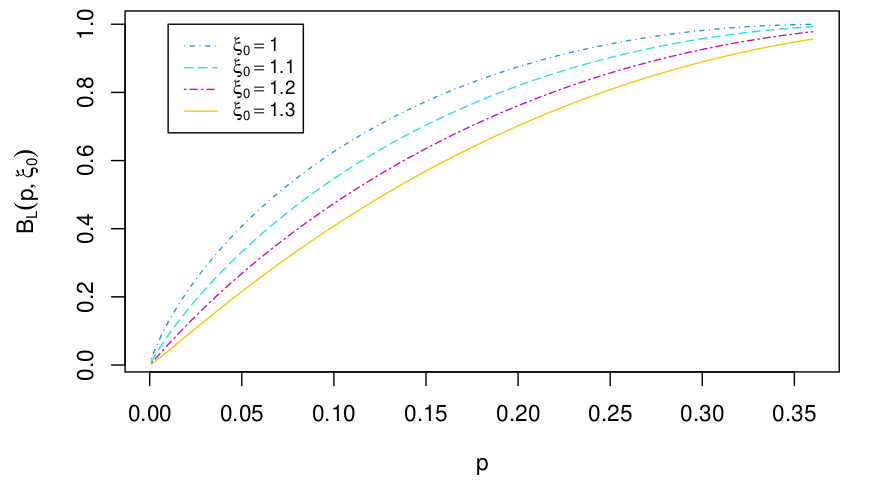
Figure 1: Graph the $RLB_{\xi_{0}}$ for different $\xi_{0}$.

In the sequel, we want to calibrate $RLB_{\xi_{0}}$ such that $RLB_{\xi_{0}}\approx B_{01}$

Lemma 1.

$B_{L}(p_{val},\xi)=-e\cdot\xi\cdot p_{val}^{\xi}\cdot\log(p_{val})\geq e\cdot\xi\cdot p_{val}^{\xi}>p_{val}^{\xi},$   for, $0<p_{val}<e^{-1}$ and $\xi\geq 1$. Note that $B_{L}(p_{val},1)=B_{L}(p_{val})$

Proof.

Let $h(p_{val})=-e\cdot\xi\cdot\log(p_{val})$, then $\dfrac{d[h(p_{val})]}{dp_{val}}=-\dfrac{e\cdot\xi}{p_{val}}<0$, thus $h$ is decreasing with minimum at $\xi=e^{-1}$. So, $h(p_{val})\geq h(e^{-1})=e\cdot\xi$ the which implies $B_{L}(p_{val},\xi)/p_{val}^{\xi}=h(p_{val})\geq e\cdot\xi,$ so $B_{L}(p_{val},\xi)\geq e\cdot\xi\cdot p_{val}^{\xi}>p_{val}^{\xi}$

∎

Theorem 1.

The $\text{RLB}_{\xi}$ is a valid $p$-value, for $\xi\geq 1$, that is,

$$P(B_{L}(p,\xi)\leq\alpha|p\sim f(p|\xi))\leq\alpha,\hskip 5.69046pt\text{for each}\hskip 5.69046pt0\leq\alpha\leq 1.$$

Proof.

First of all it can be seen that $B_{L}(p,\xi)=-e\cdot\xi\cdot p^{\xi}\cdot\log(p)$ is well defined, since $0\leq B_{L}(p,\xi)\leq 1.$

Let $\alpha\in[0,1]$, denote for $D_{B}$ the subset of $R_{p}$ (range of $p$) such that

$$-e\cdot\xi\cdot p^{\xi}\cdot\log(p)\leq\alpha,$$

then

$$(B_{L}(p,\xi)\leq\alpha)=[-e\cdot\xi\cdot p^{\xi}\cdot\log(p)\leq\alpha]=(p\in D_{B})$$

where $(p\in D_{B})$ is the event that consists of all the result $x$ such that the point $p(x)\in D_{B}$. Therefore,

$$F_{B}(\alpha)=P(B_{L}(p,\xi)\leq\alpha|p\sim f(p|\xi)) = P(-e\cdot\xi\cdot p^{\xi}\cdot\log(p)\leq\alpha|p\sim f(p|\xi))$$

$$= P(p\in D_{B}|p\sim f(p|\xi))$$

$$= \int_{D_{B}}f_{p}(p)dp$$

$$= \int_{0}^{\rho}\xi p^{\xi-1}dp$$

$$= \rho^{\xi}$$

where $\rho$ is determined such that

$$0<\rho<\frac{1}{e}\hskip 5.69046pt\text{and}\hskip 5.69046pt\alpha=-e\cdot\xi\cdot\rho^{\xi}\cdot\log(\rho)$$

as shown in the figure 2 in the case $\xi=1$

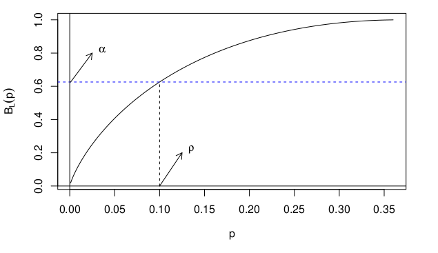
Figure 2: Plot of $B_{L}(p)$ indentifying $\rho$ such that -e$\cdot\rho\cdot\log(\rho)=\alpha$.

now, by Lemma 1 $F_{B}(\alpha)=\rho^{\xi}<-e\cdot\xi\cdot\rho^{\xi}\cdot\log(\rho)=\alpha$. ∎

2 Adaptive $\alpha$ with Strategy PBIC

An adaptive $\alpha$ allows us to adapt the statistical significance with the information, but more importantly, it allows us to arrive at equivalent results with a Bayes factor. In Pérez and Pericchi (2014) this adaptive $\alpha$ based in BIC is presented as:

$$\alpha_{n}(q)=\frac{[\chi_{\alpha}^{2}(q)+q\log(n)]^{\frac{q}{2}-1}}{2^{\frac{q}{2}-1}n^{\frac{q}{2}}\Gamma\left(\frac{q}{2}\right)}\times C_{\alpha}$$ (2)

and in Vélez et al. (2022) a version to nested linear models based in PBIC (Prior-based Bayesian Information Criterion, see Bayarri et al. (2019)) is presented as:

$$\alpha_{(b,n)}(q)=\dfrac{[g_{n,\alpha}(q)+\log(b)+C]^{\frac{q}{2}-1}}{b^{\frac{n-j}{2(n-1)}}\cdot\left(\frac{2(n-1)}{n-j}\right)^{q/2-1}\Gamma\left(\frac{q}{2}\right)}\times\exp\left\{-\frac{n-j}{2(n-1)}\left(g_{n,\alpha}(q)+C\right)\right\},$$ (3)

where $b=\frac{|\mathbf{X}_{j}^{t}\mathbf{X}_{j}|}{|\mathbf{X}_{i}^{t}\mathbf{X}_{i}|}$ and $\mathbf{X}_{i},\mathbf{X}_{j}$ are design matrix and

$$C=2\sum_{m_{i}=1}^{q_{i}}\log\frac{(1-e^{-v_{m_{i}}})}{\sqrt{2}v_{m_{i}}}-2\sum_{m_{j}=1}^{q_{j}}\log\frac{(1-e^{-v_{m_{j}}})}{\sqrt{2}v_{m_{j}}},$$

$v_{m_{l}}=\frac{\hat{\xi}_{m_{l}}}{[d_{m_{l}}(1+n^{e}_{m_{l}})]}$ with $l=i,j$ corresponding to each model. Here $n^{e}_{m_{l}}$, with $l=i,j$, refers to The Effective Sample Size (called TESS) corresponding to that parameter, see (Bayarri et al. (2019)).

If we adjust (2) replacing the constant $C_{\alpha}$ with the PBIC strategy the following expression is obtained

$$\alpha_{n}(q)=\dfrac{[\chi^{2}_{\alpha}(q)+q\log(n)+C]^{\frac{q}{2}-1}}{n^{\frac{q}{2}}2^{\frac{q}{2}-1}\Gamma\left(\frac{q}{2}\right)}\times\exp\left\{-\frac{1}{2}\left(\chi_{\alpha}^{2}(q)+C\right)\right\}.$$ (4)

Note that this adaptive $\alpha$ is still of BIC structure.

2.1 Binomial Models

Consider comparing two binomial models $S_{1}\sim binomial(n_{1},p_{1})$ and $S_{2}\sim binomial(n_{2},p_{2})$ via the test

$$H_{0}:p_{1}=p_{2}\leavevmode\nobreak\ \leavevmode\nobreak\ vs\leavevmode\nobreak\ \leavevmode\nobreak\ H_{1}:p_{1}\neq p_{2}.$$

Defining $n=n_{1}+n_{2}$ and $\hat{p}$ the MLE from $p_{1}-p_{2}$, then the equation (4) is

$$\alpha_{n}=\left[\dfrac{2}{n\pi(\chi^{2}_{\alpha}(1)+\log(n)+C)}\right]^{1/2}\times\exp\left\{-\frac{1}{2}\left(\chi_{\alpha}^{2}(1)+C\right)\right\},$$ (5)

here $\chi_{\alpha}^{2}(1)$ is the quantile $\alpha$ from chi-square with $df=1$, $C=-2\log\dfrac{(1-e^{-v})}{\sqrt{2}v}$, $v=\hat{p}^{2}/[d(1+n^{e})]$, $d=\left(\frac{\sigma_{1}^{2}}{n_{1}}+\frac{\sigma_{2}^{2}}{n_{2}}\right),n^{e}=\max\left\{\frac{n_{1}^{2}}{\sigma_{1}^{2}},\frac{n_{2}^{2}}{\sigma_{2}^{2}}\right\}d$.

The Table 1 shows the behavior $\alpha_{n}$ when $\alpha=0.5$ and $n_{1}$ and $n_{2}$ take different values.

		Adaptive $\alpha$ via PBIC ($\alpha_{n}$)
$n_{1}$	$n_{2}$	$n=n_{1}+n_{2}$
10	10	0.0068
25	25	0.0040
50	50	0.0027
100	50	0.0021
50	100	0.0021
100	100	0.0018

Table 1: Adaptive $\alpha$ via PBIC in equation 5 for testing equality of two proportions.

3 Adjusting $RLB_{\xi}$ with Adaptive $\alpha$

In this section, we use the equation (1) with the adaptive $\alpha$ in equation (3) and in equation (4) for obtaining an approximation to an objective Bayes Factor calibrating the $RLB_{\xi_{0}}$ by The Effective Sample Size (Berger et al. (2014)) and the parameters involved, according to what is established in Pericchi et al. (2017).

Using these ideas, a calibration of (1) when evaluated in (4) results in the following Bayes Factor, which has a simple expression.

$$B(\alpha,q,n,\xi_{0})=-\alpha^{\xi_{0}}\log(\alpha)\Gamma(q/2)^{\xi_{0}}n^{\frac{\xi_{0}q}{2}}\left[\dfrac{2}{\chi^{2}_{\alpha}(q)+q\cdot\log(n)+C}\right]^{\frac{\xi_{0}q}{2}-(\xi_{0}-1)}.$$ (6)

When it comes to a p-value that is not a pseudo p-value $\xi_{0}=1$ and the Bayes factor simplifies to

$$B(\alpha,q,n)=-\alpha\log(\alpha)\Gamma(q/2)n^{\frac{q}{2}}\left[\dfrac{2}{\chi^{2}_{\alpha}(q)+q\cdot\log(n)+C}\right]^{\frac{q}{2}}.$$ (7)

The refined version to linear models, for this calibration is obtained when evaluated in (3)

$$B(\alpha,q,n,b)=-\alpha\log(\alpha)\Gamma(q/2)b^{\frac{n-j}{2(n-1)}}\left[\dfrac{2(n-1)}{(g_{n,\alpha}(q)+\log(b)+C)(n-j)}\right]^{\frac{q}{2}}$$ (8)

in this case only we consider $\xi_{0}=1$ since $\alpha$ take value that are not pseudo p-value.

3.1 Balanced One Way Anova

Suppose we have $k$ groups with $r$ observations each, for a total sample size of $kr$ and let $H_{0}:\mu_{1}=\cdots=\mu_{k}=\mu\;\;vs\;\;H_{1}:\mbox{At least one }\mu_{i}\mbox{ different}$. Then the design matrices for both models are:

$$\mathbf{X}_{1}=\left(\begin{array}[]{c}1\\ 1\\ \vdots\\ 1\\ \end{array}\right)\;,\mathbf{X}_{k}=\left(\begin{matrix}1&0&\ldots&0\\ 1&0&\ldots&0\\ \vdots&\vdots&\ldots&\vdots\\ 1&0&\ldots&0\\ 0&1&\ldots&0\\ 0&1&\ldots&0\\ \vdots&\vdots&\ldots&\vdots\\ 0&1&\ldots&0\\ \vdots&\vdots&\ldots&\vdots\\ 0&0&\ldots&1\\ 0&0&\ldots&1\\ \vdots&\vdots&\ldots&\vdots\\ 0&0&\ldots&1\end{matrix}\right)\;,b=\frac{|\mathbf{X}_{k}^{t}\mathbf{X}_{k}|}{|\mathbf{X}_{1}^{t}\mathbf{X}_{1}|}=k^{-1}r^{k-1},$$

and the adaptive $\alpha$ for linear model in accordance with what was presented in Vélez et al. (2022) is

$$\alpha(k,r)=\dfrac{[g_{r,\alpha}(k-1)-\log(k)+(k-1)\log(r)+C]^{\frac{k-3}{2}}}{\left(k^{-1}r^{k-1}\right)^{\frac{r-1}{2(r-1/k)}}\left(\frac{2(r-1/k)}{r-1}\right)^{\frac{k-3}{2}}\Gamma\left(\frac{k-1}{2}\right)}\times\exp\left\{-\frac{r-1}{2(r-1/k)}\left(g_{r,\alpha}(k-1)+C\right)\right\}.$$

Here, the number of replicas $r$ is The Effective Sample Size (TESS). Therefore, the Bayes factor for this test with respect to equation (8) is:

$$B(\alpha,k,r)=-\alpha\log(\alpha)\Gamma((k-1)/2)\left(k^{-1}r^{k-1}\right)^{\frac{r-1}{2(r-1/k)}}\left[\dfrac{2(r-1/k)}{(g_{r,\alpha}(k-1)-\log(k)+(k-1)\log(r)+C)(r-1)}\right]^{\frac{k-1}{2}}$$

A very important case arises when $k=2$. For this situation, simplifies to

$$B(\alpha,r)=-\alpha\log(\alpha)\left(\dfrac{r}{2}\right)^{\frac{r-1}{2r-1)}}\left[\dfrac{2(r-1)\pi}{(g_{r,\alpha}(1)-\log\left(\dfrac{r}{2}\right)+C)(r-1)}\right]^{\frac{1}{2}}$$

4 Calibrating $P$-Values

In this section we will use (6) and (8) to determine posterior probabilities for the null hypothesis. Since for any Bayes factor $B_{01}$

$$B_{01}\geq B_{L}(p,\xi_{0})\leavevmode\nobreak\ \leavevmode\nobreak\ \leavevmode\nobreak\ \text{con}\leavevmode\nobreak\ \leavevmode\nobreak\ \leavevmode\nobreak\ \xi_{0}\geq 1,\leavevmode\nobreak\ \text{fixed but arbitrary,}$$

a lower bound for the posterior probability of the null hypothesis can be obtained as:

$$\min P(H_{0}|Data)=\left[1+\dfrac{1}{B_{L}(p,\xi_{0})}\right]^{-1}.$$ (9)

The Figure 3 shows these posterior probabilities (called $P_{RLB_{\xi_{0}}}$) for different values of $\xi_{0}$

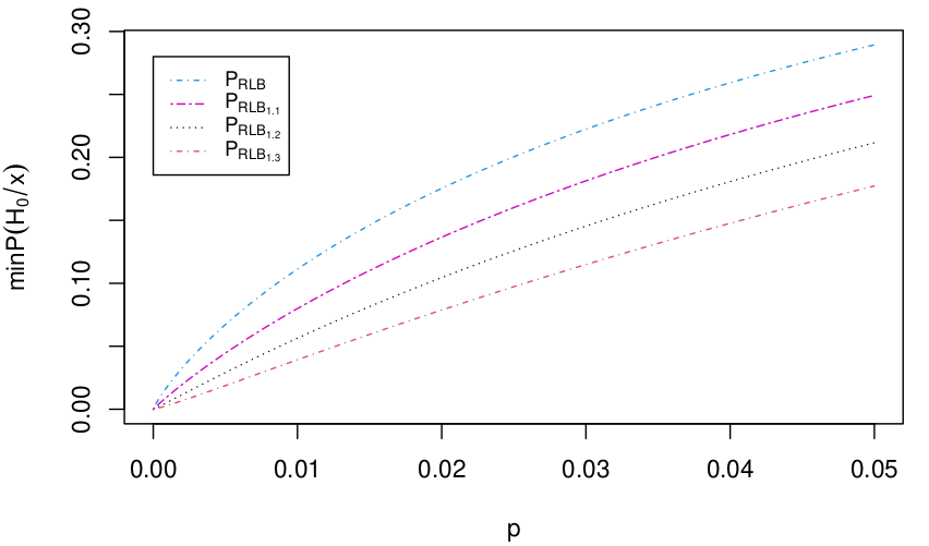
Figure 3: Lower bound for posterior probability for the null hypothesis $H_{0}$ for $\xi_{0}=1,\xi_{0}=1.1,\xi_{0}=1.2,\xi_{0}1.3$.

4.1 Testing Equality of Two Means with Unequal Variances

Consider comparing two normal means via the test

$$H_{0}:\mu_{1}=\mu_{2}\leavevmode\nobreak\ \leavevmode\nobreak\ \text{versus}\leavevmode\nobreak\ \leavevmode\nobreak\ H_{1}:\mu_{1}\neq\mu_{2},$$

where the associated known variances, $\sigma^{2}_{1}$ and $\sigma^{2}_{2}$ are not equal.

$$\mathbf{Y}=\mathbf{X}\mathbb{\mu}+\mathbb{\epsilon}=\begin{pmatrix}1&0\\ \vdots&\vdots\\ 1&0\\ 0&1\\ \vdots&\vdots\\ 0&1\end{pmatrix}\begin{pmatrix}\mu_{1}\\ \mu_{2}\end{pmatrix}+\begin{pmatrix}\epsilon_{11}\\ \vdots\\ \epsilon_{2n_{2}}\end{pmatrix},$$

$$\times\mathcal{\epsilon}\sim N(\mathbf{0},\text{diag}\{\underbrace{\sigma_{1}^{2},...,\sigma_{1}^{2}}_{n_{1}},\underbrace{\sigma_{2}^{2},...,\sigma_{2}^{2}\}}_{n_{2}})$$

Defining $\alpha=(\mu_{1}+\mu_{2})/2$ and $\beta=(\mu_{1}-\mu_{2})/2$ places this in the linear model comparison framework,

$$\mathbf{Y}=\mathbf{B}\binom{\mathbb{\alpha}}{\mathbb{\beta}}+\mathbb{\epsilon}$$

with

$$\mathbf{B}=\begin{pmatrix}1&1\\ \vdots&\vdots\\ 1&1\\ 1&-1\\ \vdots&\vdots\\ 1&-1\end{pmatrix}$$

where we are comparing $M_{0}:\beta=0$ versus $M_{1}:\beta\neq 0$.
So for (8),

$$C=-2\log\frac{(1-e^{-v})}{\sqrt{2}v}$$

$v=\frac{\hat{\beta}^{2}}{d(1+n^{e})},d=\left(\frac{\sigma_{1}^{2}}{n_{1}}+\frac{\sigma_{2}^{2}}{n_{2}}\right),n^{e}=\max\left\{\frac{n_{1}^{2}}{\sigma_{1}^{2}},\frac{n_{2}^{2}}{\sigma_{2}^{2}}\right\}\left(\frac{\sigma_{1}^{2}}{n_{1}}+\frac{\sigma_{2}^{2}}{n_{2}}\right)$.
A special case is the standard test of equality of means when $\sigma_{1}^{2}=\sigma_{2}^{2}=\sigma^{2}$. Then

$$n^{e}=\min\left\{n_{1}\left(1+\frac{n_{1}}{n_{2}}\right),n_{2}\left(1+\frac{n_{2}}{n_{1}}\right)\right\}.$$

For other hand, considering $\mu=\mu_{1}-\mu_{2}$ with $\sigma_{1}^{2}=\sigma_{2}^{2}=\sigma^{2}$

• $H_{0}:\mu_{1}=\mu_{2}\longleftrightarrow\mu=0$

• $H_{0}:\mu_{1}\neq\mu_{2}\longleftrightarrow\mu\neq 0$

Assuming priors

• $\mu|\sigma^{2},H_{1}\sim Normal(0,\sigma^{2}/\tau_{0}),\tau_{0}\in(0,\infty)$

• $\pi(\sigma^{2})\propto 1/\sigma^{2}$ for both $H_{0}$ and $H_{1}$.

The Bayes factor is:

$$BF_{01}=\left(\dfrac{n+\tau_{0}}{\tau_{0}}\right)^{1/2}\left(\dfrac{t^{2}\frac{\tau_{0}}{n+\tau_{0}}+l}{t^{2}+l}\right)^{\frac{l+1}{2}}$$

where

$$t=\frac{|\bar{\mathbf{Y}}|}{s/\sqrt{n}}$$

t-statistic with degrees of freedom $l=n-1$ and $n=n_{1}+n_{2}$ see Roger et al. (2018).

The Figure 4 shows the posterior probability for the null hypothesis $H_{0}$ when $n=50$ and $n=100$ for the Robust Lower Bound with $\xi_{0}=1$ (called $P_{RLB}$), the Bayes factor of the equation (8) (called $P_{PL}$), the Bayes factor of the equation (6) (called $P_{PG_{\xi_{0}}}$ with $\xi_{0}=1$) and for the Bayes factor $BF_{01}$ (called $P_{BF_{0.1}}$). Note that the posterior probability with $BF_{01}$ when $\tau_{0}=6$ looks very similar to the result obtained using the Bayes factors of the equations (6) and (8) .

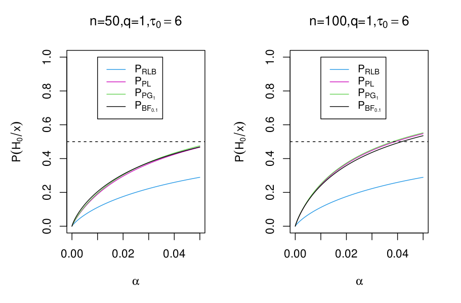
Figure 4: Posterior probability for the null hypothesis $H_{0}$ for $n=50$ and $n=100$ using the Bayes factor $RLB_{\xi_{0}}$ with $\xi_{0}=1$, the Bayes factor $BF_{01}$, the Bayes factor of the equation (7) and equation (8).

4.2 Fisher’s Exact Test

This is an example where the $p$-value is a pseudo $p$-value (see the example 8.3.30 in Casella and Berger (2001)). Let $S_{1}$ and $S_{2}$ be independent observations with $S_{1}\sim binomial(n_{1},p_{1})$ and $S_{2}\sim binomial(n_{2},p_{2})$. Consider testing $H_{0}:p_{1}=p_{2}$ vs $H_{1}:p_{1}\neq p_{2}$.
Under $H_{0}$, if we let $p$ common value of $p_{1}=p_{2}$, the joint pmf of $(S_{1},S_{2})$ is

$$f(s_{1},s_{2}|p)=\binom{n_{1}}{s_{1}}\binom{n_{2}}{s_{2}}p^{s_{1}+s_{2}}(1-p)^{n_{1}+n_{2}-(s_{1}+s_{2})}$$

and the conditional pseudo $p$-value is

$$p(s_{1},s_{2})=\sum_{j=s_{1}}^{\min\{n_{1},s\}}f(j|s),$$ (10)

the sum of hypergeometric probabilities, with $s=s_{1}+s_{2}$.

It is important to note that in Bayesian tests with point null hypothesis it is not possible to use continuous prior densities because this distributions (as well as posterior distributions) will grant zero probability to $p=(p_{1}=p_{2})$. A reasonable approximation will be to give $p=(p_{1}=p_{2})$ a positive probability $\pi_{0}$ and to $p\neq(p_{1}=p_{2})$ the prior distribution $\pi_{1}g_{1}(p)$ where $\pi_{1}=1-\pi_{0}$ and $g_{1}$ proper. One can think of $\pi_{0}$ as the mass that would be assigned to the real null hypothesis, $H_{0}:p\in((p_{1}=p_{2})-b,(p_{1}=p_{2})+b)$, if it had not been preferred to approximate by the null point hypothesis. Therefore, if

$$\pi(p)=\begin{cases}\pi_{0}&p=(p_{1}=p_{2})\\ \pi_{1}g_{1}(p)&p\neq(p_{1}=p_{2})\\ \end{cases}$$

then

$$m(s) = \int_{\Theta}f(s|p)\pi(p)dp$$

$$= f(s|(p_{1}=p_{2}))\pi_{0}+\pi_{1}\int_{p\neq(p_{1}=p_{2})}f(s|p)g_{1}(p)dp$$

$$= f(s|(p_{1}=p_{2}))\pi_{0}+(1-\pi_{0})m_{1}(s)$$

where $m_{1}(s)=\displaystyle\int_{p\neq(p_{1}=p_{2})}f(s|p)g_{1}(p)dp$ is the marginal density of $(S=S_{1}+S_{2})$ with respect to $g_{1}$.

So,

$$\pi((p_{1}=p_{2})|s)=\frac{\pi_{0}f(s|(p_{1}=p_{2}))}{m(s)}$$

thus

odds posterior $$= \dfrac{\pi((p_{1}=p_{2})|s)}{1-\pi((p_{1}=p_{2})|s)}$$

$$= \dfrac{f(s|(p_{1}=p_{2}))\pi_{0}}{m(s)(1-\dfrac{f(s|(p_{1}=p_{2}))\pi_{0}}{m(s)})}$$

$$= \dfrac{f(s|(p_{1}=p_{2}))\pi_{0}}{m(s)-f(s|(p_{1}=p_{2}))\pi_{0}}$$

$$= \dfrac{f(s|(p_{1}=p_{2}))\pi_{0}}{(1-\pi_{0})m_{1}(s)}$$

$$= \dfrac{\pi_{0}f(s|(p_{1}=p_{2}))}{\pi_{1}m_{1}(s)}$$

$$= \text{odds prior}\cdot\dfrac{f(s|(p_{1}=p_{2}))}{m_{1}(s)}$$

and the Bayes Factors is

$$B_{01}=\dfrac{f(s|(p_{1}=p_{2}))}{m_{1}(s)}.$$

Now, if we take $g_{1}(p)=Beta(a,b)$ such that $E(p)=\dfrac{a}{a+b}=(p_{1}=p_{2})$, then

$$BF_{Test}=\dfrac{B(a,b)}{B(s+a,n_{1}+n_{2}-s+b)}p^{s}(1-p)^{n_{1}+n_{2}-s}.$$

the Figure 5 shows the posterior probability for the null hypothesis $H_{0}$ when $n=n_{1}+n_{2}=50$ and $100$ for the Robust Lower Bound with $\xi_{0}=1$, the Bayes factor of the equation (6) (called $P_{PG_{\xi_{0}}}$) and for the Bayes factor $BF_{Test}$ (called $P_{BF_{Test}}$). We can note that all the $P_{PG_{\xi_{0}}}$ are comparable even though in the case $\xi_{0}=1$ it is a $p$-value and not a pseudo $p$-value.

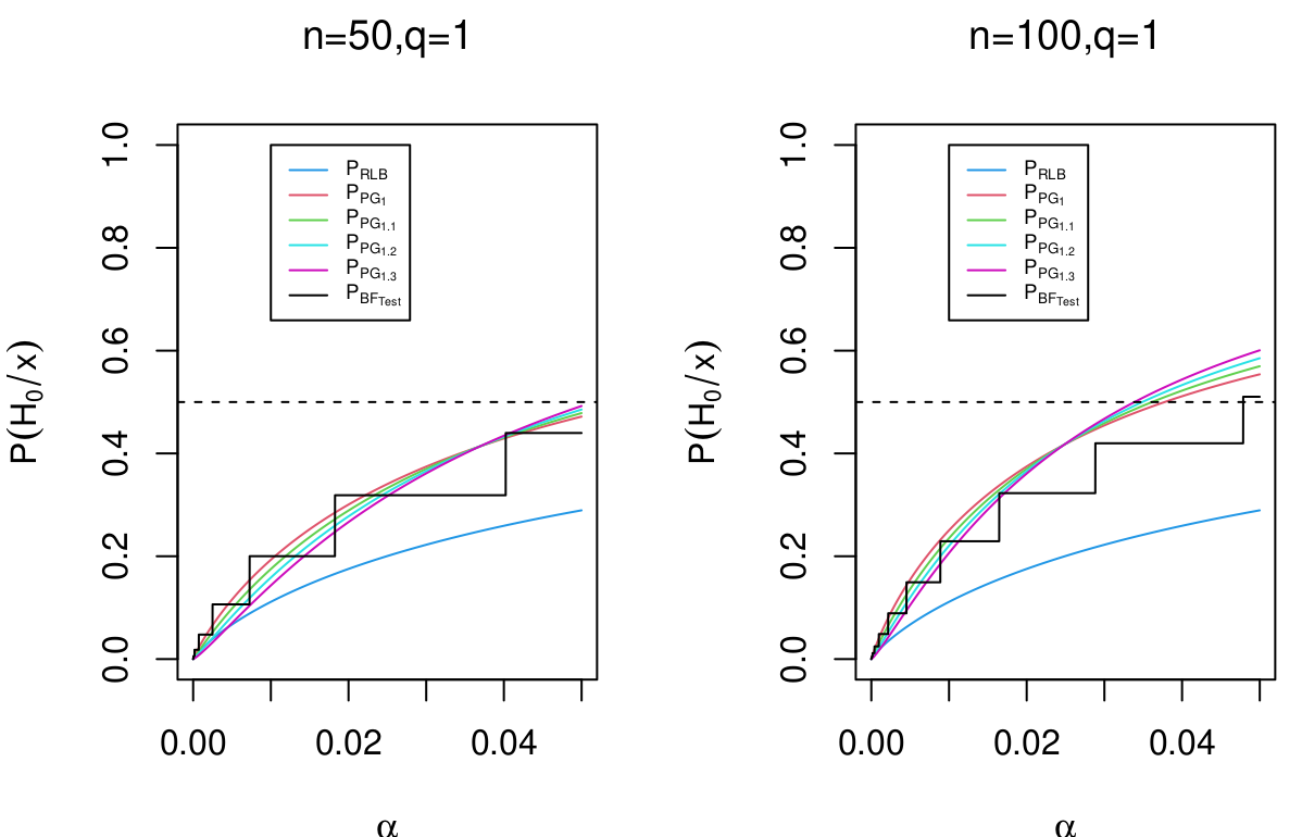
Figure 5: Posterior probability for the null hypothesis $H_{0}$ for $n=50$ and $n=100$ using the Bayes factor $RLB_{\xi_{0}}$ with $\xi_{0}=1$, the Bayes factor $BF_{Test}$ and the Bayes factor of the equation (6).

4.3 Linear Regression Models

Consider comparing two nested linear models $M_{3}:y_{l}=\beta_{1}+\beta_{2}x_{l2}+\beta_{3}x_{l3}+\epsilon_{l}$ with $M_{2}:y_{l}=\beta_{1}+\beta_{2}x_{l2}+\epsilon_{l}$ via the test

$$H_{0}:M_{2}\leavevmode\nobreak\ \leavevmode\nobreak\ \text{versus}\leavevmode\nobreak\ \leavevmode\nobreak\ H_{1}:M_{3},$$

with $1\leq l\leq n$ and the errors $\epsilon_{l}$ are assumed to be independent and normally distributed with unknown residual variance $\sigma^{2}$. According with the equation (3), in Vélez et al. (2022) and in Bayarri et al. (2019)

$$b=(n-1)s_{3}^{2}(1-\rho_{23}^{2}),$$

where $s_{3}^{2}$ is the variance $x_{v3}$ and $\rho_{23}$ is the correlation between $x_{v2}$ and $x_{v3}$, and

$$C=2\log\frac{(1-e^{-v_{2}})}{\sqrt{2}v_{2}}-2\log\frac{(1-e^{-v_{3}})}{\sqrt{2}v_{3}},$$

where $v_{2}=\hat{\beta}_{2}^{2}/[d_{2}(1+n^{e}_{2})]$, $d_{2}=\sigma^{2}/s^{2}_{x_{l2}}$, $n^{e}_{2}=s^{2}_{x_{l2}}/\max_{i}\{(x_{i2}-\bar{x}_{2})^{2}\}$ and $v_{3}=\hat{\beta}_{3}^{2}/[d_{3}(1+n^{e}_{3})]$, $d_{3}=\sigma^{2}(\stackrel{{\scriptstyle\sim}}{{X}}^{t}\stackrel{{\scriptstyle\sim}}{{X}})^{-1}$, $n_{3}^{e}=\stackrel{{\scriptstyle\sim}}{{X}}^{t}\stackrel{{\scriptstyle\sim}}{{X}}/\max_{i}\{|\stackrel{{\scriptstyle\sim}}{{X}}_{i}|^{2}\}$ with $\stackrel{{\scriptstyle\sim}}{{X}}=(\mathbf{I}_{n}-X^{*}(X^{*t}X^{*})^{-1}X^{*})x_{l3}$ and $X^{*}=(\mathbf{1}_{n}|x_{l2})$.

As an example, we analyze a data set taken from Acuna (2015) which can be accessed at http://academic.uprm.edu/eacuna/datos.html. We want to predict the average mileage per gallon (denoted by mpg) of a set of $n=82$ vehicles using four possible predictor variables: cabin capacity in cubic feet (vol), engine power (hp), maximum speed in miles per hour (sp) and vehicle weight in hundreds of pounds (wt).

Through the Bayes factors in (7) and (8) we want to choose the best model to predict the average mileage per gallon by calculating the posterior probability of the null hypothesis of the following test

$H_{0}:M_{2}:$mpg=$\beta_{1}$+$\beta_{2}\text{wt}_{l}$+$\epsilon_{l}$ vs $H_{1}:M_{3}:$mpg=$\beta_{1}$+$\beta_{2}\text{wt}_{l}$+$\beta_{3}\text{sp}_{l}$+$\epsilon_{l}$

with $\alpha=0.05$, $q=1$, $j=3$, the posterior probabilities for the null hypothesis $H_{0}$ are:

$$P_{PL}=0.9253192,P_{PG_{1}}=0.7209449$$

where $P_{PL}$ is the posterior probability associated to Bayes factor in equation (8) and $P_{PG_{1}}$ is the posterior probability associated to Bayes factor in equation (7). The use of this posterior probability in both cases will change the inference, since the $p$-value the F test is $p=0.0325$ whose is smaller than $0.05$.

4.3.1 Findley’s Counterexample

Consider the following simple linear model (Findley, 1991)

$$Y_{i}=\frac{1}{\sqrt{i}}\cdot\theta+\epsilon_{i},\leavevmode\nobreak\ \leavevmode\nobreak\ \text{where}\leavevmode\nobreak\ \epsilon_{i}\sim N(0,1),\\ i=1,2,3,..,n$$

and we are comparing the models $H_{0}:\theta=0$ and $H_{1}:\theta\neq 0$. This is a Classical and challenging counter example against BIC and the Principle of Parsimony. In Bayarri et al. (2019) it is shown the inconsistency of BIC but the consistency of PBIC in this problem.
Here we will show the posterior probabilities of the null hypothesis for this test using the Bayes factors from equations (7) and (8) when $n$ grows and $\alpha=0.05$ and $\alpha=0.01$, we will also show the posterior probabilities when $n$ fixed and $0<\alpha<0.05$. For calculations

$$C=-2\log\frac{(1-e^{-v})}{\sqrt{2}v},v=\frac{\hat{\theta}^{2}}{d(1+n^{e})},d=\left(\sum_{i=1}^{n}\frac{1}{i}\right)^{-1},n^{e}=\sum_{i=1}^{n}\frac{1}{i}$$

The Figure 6 and Figure 7 shows through posterior probability of the null hypothesis $H_{0}$ the consistency of Bayes factor based in PBIC (equation (8)), and the inconsistency of Bayes factor based in BIC (equation (7)).

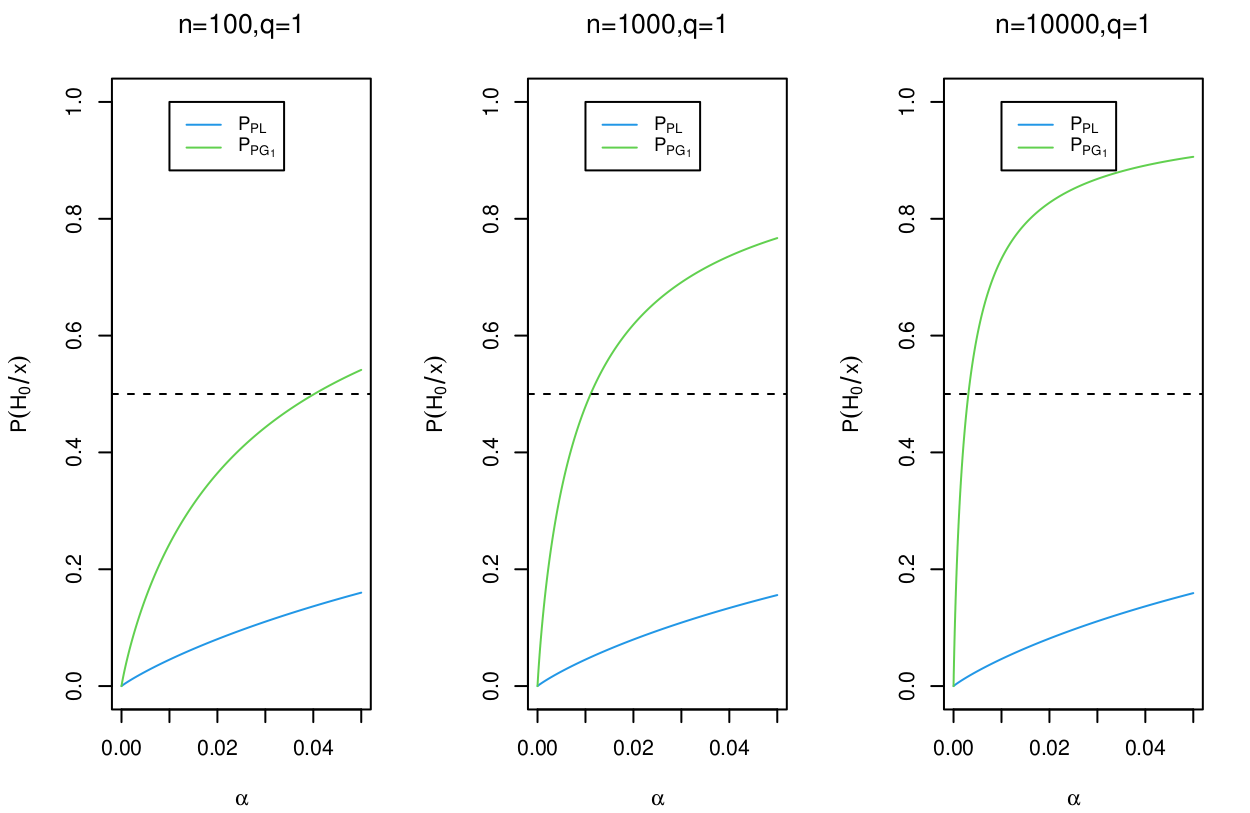
Figure 6: Posterior probability for the null hypothesis $H_{0}$ for $n=100$, $n=1000$ and $n=1000$ using the Bayes factor of the equation (7) and (8).

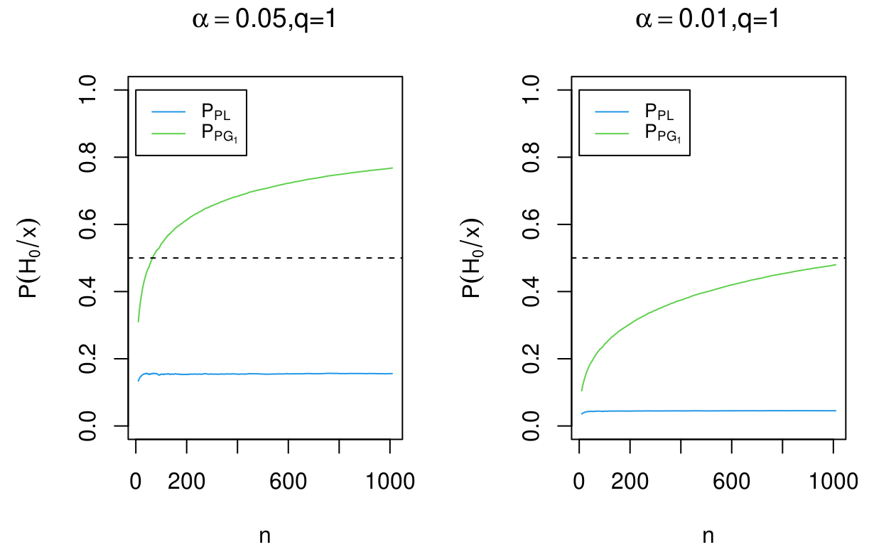
Figure 7: Posterior probability for the null hypothesis $H_{0}$ for $\alpha=0.05$ and $\alpha=0.01$ using the Bayes factor of the equation (7) and (8) when $n$ grows.

5 Discussion and Final Comments

• It will be possible to estimate the appropriate $\xi_{0}$ that best fits the pseudo p-value in (10)

• The Bayes factors (6) and (8) are simple to use and provides results equivalent to the sensitive Bayes factors of hypothesis tests whose p-value may be a pseudo p-value. We hope that this development will give tools to the practice of Statistics.

References

Acuna (2015)
Acuna, E. (2015).
Regresion Aplicada usando R.
Universidad de Puerto Rico en Mayaguez: Departamento de Ciencias
Matematicas.
Bayarri et al. (2019)
Bayarri, M. J., J. O. Berger, W. Jang, S. Ray, L. R. Pericchi, and I. Visser
(2019).
Prior-based bayesian information criterion.
Statistical Theory and Related Fields3(1), 2–13.
Berger
et al. (2014)
Berger, J., M. J. Bayarri, and L. R. Pericchi (2014).
The effective sample size.
Econometric Reviews33(1-4), 197–217.
Casella and
Berger (2001)
Casella, G. and R. Berger (2001).
Statistical Inference (2nd ed.).
Duxbury Resource Center.
Findley (1991)
Findley, D. F. (1991).
Counterexamples to parsimony and BIC.
Ann Inst Stat Math43, 505–514.
Held and Ott (2018)
Held, L. and M. Ott (2018).
On -values and bayes factors.
Annual Review of Statistics and Its Application5,
393–419.
Pérez and
Pericchi (2014)
Pérez, M. E. and L. R. Pericchi (2014).
Changing statistical significance with the amount of information: The
adaptive alfa significance level.
Statistics and Probability Letters85, 20–24.
Pericchi
et al. (2017)
Pericchi, L. R., M. Pérez, and D. Vélez (2017).
Converting p-values in posterior probabilities to increase the
reproducible scientific “finding".
arXiv:1711.06219.
Roger
et al. (2018)
Roger, S. Z., A. Sarkar, R. J. Carroll, and B. K. Mallick (2018).
A powerful bayesian test for equality of means in high dimensions.
Journal of the American Statistical Association113(524), 1733–1741.
Sellke
et al. (2001)
Sellke, T., M. J. Bayarri, and J. O. Berger (2001).
Calibration of p values for testing precise null hypotheses.
The American Statistician55(1), 62–71.
Vélez et al. (2022)
Vélez, D., M. E. Pérez, and L. R. Pericchi (2022, feb).
Increasing the replicability for linear models via adaptive
significance levels.
TEST.
Vovk (1993)
Vovk, V. (1993).
A logic of probability, with application to the foundations of
statistic.
Journal Royal Statistical SocietySeries B(55),
317–351.