Physics-Informed Deep Monte Carlo Quantile Regression method for Interval Multilevel Bayesian Network-based Satellite Heat Reliability Analysis

Abstract

Temperature field reconstruction is essential for analyzing satellite heat reliability. As a representative machine learning model, the deep convolutional neural network (DCNN) is a powerful tool for reconstructing the satellite temperature field. However, DCNN needs a lot of labeled data to learn its parameters, which is contrary to the fact that actual satellite engineering can only acquire noisy unlabeled data. To solve the above problem, this paper proposes an unsupervised method, i.e., the physics-informed deep Monte Carlo quantile regression method, for reconstructing temperature field and quantifying the aleatoric uncertainty caused by data noise. For one thing, the proposed method combines a deep convolutional neural network with the known physics knowledge to reconstruct an accurate temperature field using only monitoring point temperatures. For another thing, the proposed method can quantify the aleatoric uncertainty by the Monte Carlo quantile regression. Based on the reconstructed temperature field and the quantified aleatoric uncertainty, this paper models an interval multilevel Bayesian Network to analyze satellite heat reliability. Two case studies are used to validate the proposed method.

1 Introduction

As an important aircraft in aerospace engineering [1, 2], the components’ working power of satellite will fluctuate due to some uncertainty factors like the manufacture defects, the different orbital environments, etc. Thereby, it will lead to changes in the temperature fields of some satellite subsystems. If the temperature is too high, it will significantly influence the satellite performance and even cause the satellite to malfunction. Therefore, the heat reliability analysis is essential for analyzing the effects of uncertainty factors on the satellite system performance and minimizing the failure risk [3, 4, 5].

In actual satellite engineering, only a limited number of temperature monitoring sensors are placed on satellites to save expensive satellite payloads and rare space on circuit boards. However, only engineers who know the temperature at any point on the satellite component can perform an accurate heat reliability analysis. To solve this problem, the surrogate model needs to be built to reconstruct the temperature field of the entire satellite subsystem based on a limited number of monitoring point temperatures. Then, the temperature at any point on the satellite component is obtained according to the reconstructed temperature field. Many methods have been studied to construct the surrogate model in recent years, such as the polynomial chaos expansion method [6, 7, 8, 9], the Gaussian process regression method [10, 11], the support vector machine method [12, 13, 14], the Kriging method [9, 15, 16], etc. These methods are suitable for low-dimensional regression problems. However, the satellite temperature field reconstruction (TFR) is a high-dimensional image-to-image regression problem in this paper. As a representative machine learning model, the deep convolutional neural network (DCNN) has drawn a lot of researches in many fields [17, 18, 19, 20]. Due to the convolution operation can reduce the amount of calculation by associating some neurons, DCNN can construct an accurate surrogate model for high-dimensional image-to-image regression problems. Thus, this paper uses DCNN to build a surrogate model for reconstructing the temperature field of the satellite subsystem.

In recent years, plenty of methods has been studied for constructing a surrogate model based on DCNN. The DCNN-based surrogate model construction methods mainly include the ship-ship collision risk classification method[18], the time-frequency information signal prediction method[11], the associated remaining useful life estimation method[21], the accident prediction method of highway-rail grade crossing[22], the sensor network modeling method[23], the uncertainty quantification method of blood flow[24], etc. For these methods, the common feature is that they all need a lot of labeled data to learn the parameters of DCNN models. However, due to the high cost of acquiring data labels, some engineering problems only have a small amount of labeled data or even have just some unlabeled data. For satellite engineering, only some monitoring point temperatures can be acquired by a limited number of sensors, and the truth temperature field of the satellite subsystem is hard and expensive to obtain. Therefore, one of the difficulties for the satellite TFR problem is constructing an accurate DCNN model by some monitoring point temperatures.

To overcome the problem of insufficient labeled training data, DCNN combined with the known physical knowledge, such as partial differential equations, boundary and initial conditions, etc., results in a physics-informed DCNN model used to construct surrogate models in different problems. Shen et al.[25] proposed a physics-informed DCNN model by a simple threshold model for bearing fault detection. For solving partial differential equations, Fang [26] developed a hybrid physics-informed DCNN model based on finite volume methods. Besides, Gao et al. [27, 28] proposed a novel physics-informed DCNN learning framework to solve partial differential equations on irregular domains. Combined with the topology optimization knowledge, Zhang et al. [29] studied a topology optimization via neural reparameterization framework using physics-informed DCNN. In summary, the above problems make full use of the known physical knowledge to reduce the amount of labeled data when DCNN is used to construct a high-precision surrogate model. For the satellite TFR problem, the steady-state temperature field satisfies the Laplace equation and some boundary conditions [19]. Besides, the adjacent temperature value in the steady-state temperature field will not mutate sharply, which means that the steady-state temperature field obeys the TV regularization rule [30, 31]. Based on the known physical knowledge, this paper proposes a physics-informed DCNN model to reconstruct the temperature field of the satellite subsystem by some monitoring point temperatures.

In actual satellite engineering, the monitoring point temperatures are measured by temperature sensors. However, the possible measure drift of the sensor will lead to data noise existing in the monitoring point temperatures. Thus, when the physics-informed DCNN model reconstructs the temperature field of the satellite subsystem by the monitoring point temperatures with noises, there is aleatoric uncertainty in the reconstructed temperature field. If the aleatoric uncertainty is ignored, the reconstructed temperature field will not be accurate. Sequentially, the final satellite heat reliability analysis results will also be unbelievable. Thereby, another difficulty for the satellite TFR problem is quantifying the aleatoric uncertainty caused by the data noise. Some researchers have studied the aleatoric uncertainty quantification method. Based on a Gaussian maximum-likelihood formulation of a neural network, Nix and Weigend [32] proposed an architecture for a network with one output unit and one variance unit, where the variance unit is used to quantify aleatoric uncertainty. Based on this method, Kendall and Gal [33] studied aleatoric uncertainty quantification for classification Tasks by DCNN. Both the above two approaches are limited by Gaussian assumption [32]. Combined with quantile regression, Tagasovska and Lopez-Paz [34] proposed a simultaneous quantile regression (SQR) method to estimate aleatoric uncertainty. However, the SQR method is not suitable for the image-to-image regression problem. For the satellite TFR problem, this paper proposes a Monte Carlo quantile regression method to quantify the aleatoric uncertainty caused by data noise based on quantile regression.

In summary, the proposed physics-informed DCNN model combined with the proposed Deep MC-QR method results in a physics-informed deep Monte Carlo quantile regression (Deep MC-QR) method. The main innovations of the proposed physics-informed Deep MC-QR method are twofold: (1) This paper proposes a physics-informed DCNN model to construct a satellite TFR surrogate model using only monitoring point temperatures. (2) This paper proposes a Deep MC-QR method to quantify the aleatoric uncertainty caused by data noise based on the Monte Carlo quantile regression. In this paper, the parameters involved in the physics-informed Deep MC-QR method are learned by the proposed MC iterative training algorithm. After that, the satellite subsystem temperature field and the corresponding aleatoric uncertainty can be estimated by the proposed Satellite TFR and aleatoric uncertainty quantification algorithm.

This paper constructs the interval temperature field using the reconstructed satellite subsystem temperature field and the corresponding aleatoric uncertainty to make the satellite heat reliability analysis more believable. According to the work state thresholds of satellite components, the normal probability intervals of satellite components can be obtained by implementing the Monte Carlo simulation on the trained physics-informed Deep MC-QR model. Many methods have been studied for system reliability inference in recent years, such as Bayesian Network (BN) [4, 35, 36, 37], Universal Generate Function [38, 39], Fault Tree Analysis [40, 41], Binary Decision Diagram [42, 43], etc. This paper chooses BN to infer the satellite heat reliability. According to the components’ normal probability intervals and the satellite subsystem hierarchical structure, the heat reliability inference model is built to be an interval multilevel BN. Then, this paper derives the normal probability interval calculation formula for the child node whose logical relationship is series or parallel, based on which the interval multilevel BN can infer the satellite heat reliability.

The rest of this paper is organized as follows. In section 2, the theoretical bases including DCNN and quantile regression are introduced. Then, the physics-informed Deep MC-QR method for satellite TFR is proposed in section 3. Using the reconstructed temperature field and quantified aleatoric uncertainty, the satellite heat reliability analysis method is proposed based on interval multilevel BN in section 4. In section 5, the first case study is used to validate that the proposed physics-informed Deep MC-QR method can accurately reconstruct satellite temperature field and quantify the aleatoric uncertainty, and the proposed methods are applied to the heat reliability analysis for a satellite subsystem in the second case study.

2 Theoretical bases

2.1 Deep convolutional neural network

Definition of DCNN

DCNN is a deep neural network that includes convolutional layers [44]. The DCNN adopted in this paper uses the two-dimensional convolutional layer. The $l\text{th}$ two-dimensional convolutional layer performs convolution operations on the $l\text{th}$ two-dimensional layer input $\bm{I}^{l}$ and the convolution kernel $\bm{K}^{l}$ and adds a scalar bias $b^{l}$ to obtain the output $\bm{S}^{l}$, i.e.,

$$\bm{S}^{l}\left(i,j\right)=\left(\bm{I}^{l}*\bm{K}^{l}\right)\left(i,j\right)+b^{l}$$ (1)

$$\qquad\quad=\sum\limits_{u}{\sum\limits_{v}{\bm{I^{l}}\left(u,v\right)\bm{K}^{l}\left(i-u,j-v\right)}}+b^{l},$$

where $\bm{S}^{l}\left(i,j\right)$ represents the element in the $i\text{th}$ row and $j\text{th}$ column of $\bm{S}^{l}$, $*$ denotes the convolution operation. Then, the output $\bm{S}^{l}$ is input to the nonlinear activation layer to get the activation value $\bm{H}^{l}$, i.e.,

$$\bm{H}^{l}\left(i,j\right)=g\left[\bm{S}^{l}\left(i,j\right)\right],$$ (2)

where $g$ is the nonlinear activation function [45]. In addition, DCNN usually uses a pooling layer (e.g., max-pooling [46]) to help the representation of layer input be approximately invariant[44].

For a DCNN, the parameters $\bm{\theta}=\left(\bm{K},\bm{b}\right)$ need to be learned by minimizing the loss function $\mathcal{L}\left(\theta\right)$, i.e.,

$$\bm{\theta}^{*}=\arg\min\mathcal{L}\left(\bm{\theta}\right),$$ (3)

where $\mathcal{L}\left(\theta\right)$ can be the mean absolute error or the mean square error[47].

U-net

This paper uses a classical DCNN U-net [20], which can process large images and capture the detailed characteristics of the images. The architecture of U-net is shown in Fig.1, including two parts, i.e., the encoder part (Conv1, Conv2, Conv3, Conv4, Conv5) and the decoder part (Upconv1, Upconv2, Upconv3, Upconv4), where the encoder part extracts the image’s feature, and the decoder part gradually samples the feature image to the target output image’s size. The green cuboid contains convolution calculation, batch normalization, and ReLU [45]. The purple cuboid is the downsample achieved by the max-pooling operation [46]. The orange cuboid is the upsample implemented by the deconvolution operation [48]. The other detailed information of the U-net can refer to this document [20].

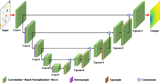
Figure 1: The architecture of U-net.

2.2 Quantile Regression

For a stochastic system $W=f\left(\bm{V}\right)$ with the random input variable $\bm{V}$, supposed that the cumulative distribution function of the output $W$ taking the value $w$ is

$${{F}_{W|\bm{V}=\bm{v}}}\left(w|\bm{v}\right)=P\left(W\leq w\right).$$ (4)

Thus, the $\tau$ quantile of the output $W$ is

$${{Q}_{\tau}}\left(W|\bm{V}=\bm{v}\right)=\arg\inf\left\{w\in\mathbb{R};{{F}_{W|\bm{V}=\bm{v}}}\left(w|\bm{v}\right)>\tau\right\},$$ (5)

where $\tau$ ($0\leq\tau\leq 1$) is the quantile level. If the inverse function of ${{F}_{W|\bm{V}=\bm{v}}}\left(w|\bm{v}\right)$ is $F_{W|\bm{V}=\bm{v}}^{-1}\left(\tau\right)$,

$${{Q}_{\tau}}\left(W|\bm{V}=\bm{v}\right)=F_{W|\bm{V}=\bm{v}}^{-1}\left(\tau\right).$$ (6)

For the quantile level $\tau$, the goal of quantile regression is to build a surrogate model $\hat{W}={{\hat{f}}_{\tau}}\left(\bm{V}\right)$ of $W=f\left(\bm{V}\right)$. Based on the training data set $\left\{\left({{\bm{v}}_{i}},{{w}_{i}}\right)|i=1,2,\cdots,N\right\}$, the pinball loss function [49, 34] was proposed, i.e.,

$${{l}_{\tau}}\left[{{w}_{i}},{{{\hat{f}}}_{\tau}}\left({{\bm{v}}_{i}}\right)\right]=\left\{\begin{matrix}\tau\left({{w}_{i}}-{{{\hat{w}}}_{i}}\right),&{{w}_{i}}\geq{{{\hat{w}}}_{i}}\\ \left(1-\tau\right)\left({{{\hat{w}}}_{i}}-{{w}_{i}}\right),&{{w}_{i}}<{{{\hat{w}}}_{i}}\\ \end{matrix}\right.$$ (7)

$$\mathcal{L}\left[{{w}_{i}},{{{\hat{f}}}_{\tau}}\left(\bm{v}_{i}\right)\right]=\frac{1}{N}\sum\limits_{i=1}^{N}{{{l}_{\tau}}\left[{{w}_{i}},{{{\hat{f}}}_{\tau}}\left({{\bm{v}}_{i}}\right)\right]},$$

where ${{\hat{w}}_{i}}={{\hat{f}}_{\tau}}\left({{\bm{v}}_{i}}\right)$ is the prediction corresponding to the input $\bm{v}_{i}$. By minimizing the loss function, i.e.,

$${{\hat{f}}_{\tau}}\left(\bm{V}\right)=\arg\min\mathcal{L}\left[w,{{{\hat{f}}}_{\tau}}\left(\bm{v}\right)\right],$$ (8)

the surrogate model $\hat{W}={{\hat{f}}_{\tau}}\left(\bm{V}\right)$ can be built to approximate $W=f\left(\bm{V}\right)$.

3 Physics-informed Deep MC-QR method for satellite TFR

3.1 Satellite TFR problem

As shown in Fig.2(a), a satellite subsystem with $n$ components $\left\{C_{s}|s=1,2,\cdots,n\right\}$ is simplified into a two-dimensional square area $\Omega$ with side length $L$, where the powers of $n$ components are $\left\{P_{s}|s=1,2,\cdots,n\right\}$. The gray grid shaded area is adiabatic. Besides, the yellow rectangle with width $\delta$ at the top is the position of the heat sink. The temperature of each point at the junction (red line, denoted as ${\Omega}_{BC}$) of square area $\Omega$ and heat sink is a constant $T_{0}$. In Fig.2(b), the red points are the positions of temperature monitoring sensors. It is noted that the number of temperature monitoring sensors and their locations need to be determined according to the studied specific satellite subsystem.

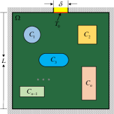
(a) Satellite subsystem component layout

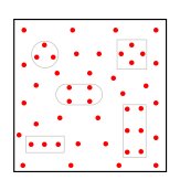
(b) Temperature monitoring point position

Figure 2: Simplified modeling of a satellite subsystem with $n$ components in a two-dimensional square area.

For the heat conduction of two-dimensional square area $\Omega$, its steady state temperature field $\bm{T}$ meets the Laplace equation [19, 31], i.e.,

$$\frac{{{\partial}^{2}}\bm{T}\left(x,y\right)}{\partial{{x}^{2}}}+\frac{{{\partial}^{2}}\bm{T}\left(x,y\right)}{\partial{{y}^{2}}}+\bm{\varphi}\left(x,y\right)=0,\quad\left(x,y\right)\in\Omega,$$ (9)

and the boundary condition

$$\bm{T}\left(x,y\right)={{T}_{0}},\quad\left(x,y\right)\in{{\Omega}_{BC}}$$ (10)

where $\left(x,y\right)$ denotes the position coordinate and $\bm{\varphi}$ is the heat source intensity distribution determined by the component power. For the satellite TFR problem, the heat source intensity distribution $\bm{\varphi}$ is unknown. Thus, the satellite TFR problem only considers the heat conduction in areas without components. The Laplace equation in Eq.(9) can be simplified to

$$\frac{{{\partial}^{2}}\bm{T}\left(x,y\right)}{\partial{{x}^{2}}}+\frac{{{\partial}^{2}}\bm{T}\left(x,y\right)}{\partial{{y}^{2}}}=0,\quad\left(x,y\right)\in{{\Omega}_{NC}},$$ (11)

where ${\Omega}_{NC}$ denotes the area without components.

As shown in Fig.3, the goal of satellite TFR problem is to build a surrogate model $\mathcal{M}\left(\bm{T}_{MP}\right)$ that can reconstruct the temperature field of the satellite subsystem (Fig.2(a)) by the monitoring point (MP) temperature image $\bm{T}_{MP}$ (Fig.2(b)). For the MP temperature image $\bm{T}_{MP}$, the values of the red points are the temperature monitoring sensors’ values, and the other points’ values are all zero.

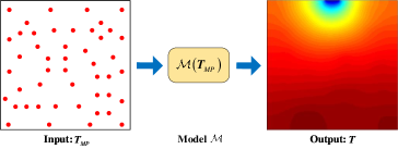
Figure 3: The satellite TFR problem.

3.2 Physics-informed Deep MC-QR model

For the satellite TFR problem, this section proposes a physics-informed Deep MC-QR model to reconstruct the temperature field and quantify the aleatoric uncertainty caused by data noise, as shown in Fig.4. The input $\left({{\bm{T}}_{MP}},\bm{\tau}\right)$ consists of the MP temperature image $\bm{T}_{MP}$ and the quantile level image $\bm{\tau}$. In this paper, the MP temperature image $\bm{T}_{MP}$ is discretized to be a ${{H}_{\Omega}}\times{{W}_{\Omega}}$ two-dimensional array. Besides, the quantile level image ${{H}_{\Omega}}\times{{W}_{\Omega}}$ is also a two-dimensional array $\bm{\tau}$. If $\left(x,y\right)\in{\Omega}_{MP}$, the corresponding position’s value $\bm{\tau}\left(x,y\right)$ is equal to $\tau$ ($\tau\sim U\left(0,1\right)$), i.e.,

$$\forall\left(x,y\right)\in{\Omega}_{MP},\quad\tau\sim U\left(0,1\right),\quad\bm{\tau}\left(x,y\right)={\tau},$$ (12)

where ${\Omega}_{MP}$ denotes the set of temperature monitoring sensors’ positions in the discretized temperature image $\bm{T}_{MP}$. Otherwise, the rest elements of the array $\bm{\tau}$ are equal to zero. As shown in Fig.4, the values of all blue points in the quantile level image $\bm{\tau}$ are equal to $\tau$, and the other points’ values are zero.

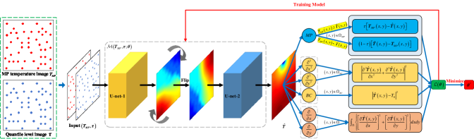
Figure 4: The schematic of physics-informed Deep Monte Carlo quantile regression model.

In Fig.4, the first DCNN U-net-1 extracts the feature map of input $\left({{\bm{T}}_{MP}},\bm{\tau}\right)$. Besides, the feature map is flipped diagonally to ensure the reconstruction accuracy of temperature field in the upside and right-side boundaries [31]. Then, the second DCNN U-net-2 uses the flipped feature map to predict the temperature field $\hat{\bm{T}}$ of the satellite subsystem. Therefore, two U-net models (U-net-1 and U-net-2) and diagonal flip operation build the physics-informed Deep MC-QR model $\mathcal{M}\left(\bm{T}_{MP},\bm{\tau};\bm{\theta}\right)$, where $\bm{\theta}$ are the parameters of two U-net models. The training of model $\mathcal{M}\left(\bm{T}_{MP},\bm{\tau};\bm{\theta}\right)$ is informed by the quantile MP temperature error, the Laplace equation (Eq.(11)), the boundary condition (Eq.(10)), and the total variation (TV) regularization [30, 50].

Supposed that $N_{MP}$ temperature monitoring sensors are placed at the appropriate positions of satellite subsystem in Fig.2(a). Given $N$ MP temperature images $\left\{\bm{T}^{i}_{MP}|i=1,2,\cdots,N\right\}$, the parameters $\bm{\theta}$ are learned by minimizing the proposed physics-informed loss function $\mathcal{L}\left(\theta\right)$, consisting of the quantile MP temperature mean error $\mathcal{L}_{\tau}\left(\bm{\theta}\right)$, the Laplace equation mean squared error $\mathcal{L}_{LE}\left(\bm{\theta}\right)$, the boundary condition mean squared error $\mathcal{L}_{BC}\left(\bm{\theta}\right)$ and the TV regularization $\mathcal{L}_{TV}\left(\bm{\theta}\right)$.

• Quantile MP temperature mean error $\mathcal{L}_{\tau}\left(\bm{\theta}\right)$

For the $i\text{th}$ MP temperature image $\bm{T}^{i}_{MP}$, the predicted temperature field $\hat{\bm{T}}$ of the satellite subsystem is

$${\hat{\bm{T}}_{i}}=\mathcal{M}\left(\bm{T}^{i}_{MP},\bm{\tau}_{i};\bm{\theta}\right).$$ (13)

For $\left(x,y\right)\in{\Omega}_{MP}$, the error ${{l}_{{\tau}_{i}}}\left(x,y;\bm{\theta}\right)$ is

$${{l}_{{\tau}_{i}}}\left(x,y;\bm{\theta}\right)=\left\{\begin{matrix}{\tau}_{i}\left[{{\bm{T}^{i}_{MP}}\left(x,y\right)}-{{\hat{\bm{T}_{i}}}\left(x,y\right)}\right],&{{\bm{T}^{i}_{MP}}\left(x,y\right)}\geq{{\hat{\bm{T}_{i}}}\left(x,y\right)}\\ \left(1-{\tau}_{i}\right)\left({{\hat{\bm{T}_{i}}}\left(x,y\right)}-{{\bm{T}^{i}_{MP}}\left(x,y\right)}\right),&{{\bm{T}^{i}_{MP}}\left(x,y\right)}<{{\hat{\bm{T}_{i}}}\left(x,y\right)}\\ \end{matrix}\right.,$$ (14)

where ${\tau}_{i}\sim U\left(0,1\right)$. For $N$ MP temperature images $\left\{\bm{T}^{i}_{MP}|i=1,2,\cdots,N\right\}$, the quantile MP temperature mean error $\mathcal{L}_{\tau}\left(\bm{\theta}\right)$ is

$$\mathcal{L}_{\tau}\left(\bm{\theta}\right)=\frac{1}{N}\frac{1}{N_{MP}}\sum\limits_{i=1}^{N}{\sum_{\left(x,y\right)\in{\Omega}_{MP}}{{{l}_{{\tau}_{i}}}\left(x,y;\bm{\theta}\right)}}.$$ (15)

• Laplace equation mean squared error $\mathcal{L}_{LE}\left(\bm{\theta}\right)$

Suppose that each discretized MP temperature image $\bm{T}^{i}_{MP}$ has $N_{NC}$ points satisfying the condition $\left(x,y\right)\in{{\Omega}_{NC}}$. According to Eq.(11), the Laplace equation mean squared error $\mathcal{L}_{LE}\left(\bm{\theta}\right)$ for $N$ MP temperature images $\left\{\bm{T}^{i}_{MP}|i=1,2,\cdots,N\right\}$ is

$${{\mathcal{L}}_{LE}}\left(\bm{\theta}\right)=\frac{1}{N}\frac{1}{{{N}_{NC}}}\sum\limits_{i=1}^{N}{\sum\limits_{\left(x,y\right)\in{{\Omega}_{NC}}}{{{\left|\frac{{{\partial}^{2}}\hat{\bm{T}}_{i}\left(x,y\right)}{\partial{{x}^{2}}}+\frac{{{\partial}^{2}}\hat{\bm{T}}_{i}\left(x,y\right)}{\partial{{y}^{2}}}\right|}^{2}}}}.$$ (16)

By discretizing the Laplace equation Eq.(11), the first part ${{\partial}^{2}}\hat{\bm{T}}_{i}\left(x_{j},y_{k}\right)/{\partial{{x}_{j}^{2}}}$ for position coordinate $\left(x_{j},y_{k}\right)$ can be

$$\frac{{{\partial}^{2}}\hat{\bm{T}}_{i}\left(x_{j},y_{k}\right)}{\partial{{x}_{j}^{2}}}=\frac{{\left[\hat{\bm{T}}_{i}\left({{x}_{j+1}},{{y}_{k}}\right)-\hat{\bm{T}}_{i}\left({{x}_{j}},{{y}_{k}}\right)\right]}/{\left({{x}_{j+1}}-{{x}_{j}}\right)-{\left[\hat{\bm{T}}_{i}\left({{x}_{j}},{{y}_{k}}\right)-\hat{\bm{T}}_{i}\left({{x}_{j-1}},{{y}_{k}}\right)\right]}/{\left({{x}_{j}}-{{x}_{j-1}}\right)}\;}\;}{{{x}_{j}}-{{x}_{j-1}}}.$$ (17)

Denoted that $\Delta{{x}_{j}}={{x}_{j}}-{{x}_{j-1}}$ and $\Delta{{\hat{\bm{T}}}^{i}_{j}}=\hat{\bm{T}}_{i}\left({{x}_{j}},{{y}_{k}}\right)-\hat{\bm{T}}_{i}\left({{x}_{j-1}},{{y}_{k}}\right)$. Then, Eq.(17) can be

$$\frac{{{\partial}^{2}}\hat{\bm{T}}_{i}\left(x_{j},y_{k}\right)}{\partial{{x}_{j}^{2}}}=\frac{{\Delta{{{\hat{\bm{T}}}}^{i}_{j+1}}}/{\Delta{{x}_{j+1}}-{\Delta{{{\hat{\bm{T}}}}^{i}_{j}}}/{\Delta{{x}_{j}}}\;}\;}{\Delta{{x}_{j}}}$$ (18)

$$\qquad\qquad\quad\;\,=\frac{\Delta{{{\hat{\bm{T}}}}^{i}_{j+1}}\Delta{{x}_{j}}-\Delta{{{\hat{\bm{T}}}}^{i}_{j}}\Delta{{x}_{j+1}}}{\Delta{{x}_{j+1}}{{\Delta}^{2}}{{x}_{j}}}.$$

Like Eq.(18), the second part ${{\partial}^{2}}\hat{\bm{T}}_{i}\left(x_{j},y_{k}\right)/{\partial{{y}_{k}^{2}}}$ of Eq.(11) can be

$$\frac{{{\partial}^{2}}\hat{\bm{T}}_{i}\left({{x}_{j}},{{y}_{k}}\right)}{y_{k}^{2}}=\frac{{\Delta{{{\hat{\bm{T}}}}^{i}_{k+1}}}/{\Delta{{y}_{k+1}}-{\Delta{{{\hat{\bm{T}}}}^{i}_{k}}}/{\Delta{{y}_{k}}}\;}\;}{\Delta{{y}_{k}}}$$ (19)

$$\qquad\qquad\quad\;\,=\frac{\Delta{{{\hat{\bm{T}}}}^{i}_{k+1}}\Delta{{y}_{k}}-\Delta{{{\hat{\bm{T}}}}^{i}_{k}}\Delta{{y}_{k+1}}}{\Delta{{y}_{k+1}}{{\Delta}^{2}}{{y}_{k}}},$$

where $\Delta{{y}_{k}}={{y}_{k}}-{{y}_{k-1}}$ and $\Delta{{\hat{\bm{T}}}^{i}_{k}}=\hat{\bm{T}}_{i}\left({{x}_{j}},{{y}_{k}}\right)-\hat{\bm{T}}_{i}\left({{x}_{j}},{{y}_{k-1}}\right)$. Refer to Eqs.(18) and (19), Eq.(16) is further transformed into

$${{\mathcal{L}}_{LE}}\left(\bm{\theta}\right)=\frac{1}{N}\frac{1}{{{N}_{NC}}}\sum\limits_{i=1}^{N}{\sum\limits_{\left(x,y\right)\in{{\Omega}_{NC}}}{{{\left|\frac{\Delta{{{\hat{\bm{T}}}}^{i}_{j+1}}\Delta{{x}_{j}}-\Delta{{{\hat{\bm{T}}}}^{i}_{j}}\Delta{{x}_{j+1}}}{\Delta{{x}_{j+1}}{{\Delta}^{2}}{{x}_{j}}}+\frac{\Delta{{{\hat{\bm{T}}}}^{i}_{k+1}}\Delta{{y}_{k}}-\Delta{{{\hat{\bm{T}}}}^{i}_{k}}\Delta{{y}_{k+1}}}{\Delta{{y}_{k+1}}{{\Delta}^{2}}{{y}_{k}}}\right|}^{2}}}}.$$ (20)

• Boundary condition mean squared error $\mathcal{L}_{BC}\left(\bm{\theta}\right)$

Assume that there are $N_{BC}$ points $\left(x,y\right)$ in the area ${{\Omega}_{BC}}$ of each discretized MP temperature image $\bm{T}^{i}_{MP}$. Refer to Eq.(10), the boundary condition mean squared error $\mathcal{L}_{BC}\left(\bm{\theta}\right)$ for $N$ MP temperature images $\left\{\bm{T}^{i}_{MP}|i=1,2,\cdots,N\right\}$ is

$${{\mathcal{L}}_{BC}}\left(\bm{\theta}\right)=\frac{1}{N}\frac{1}{{{N}_{BC}}}\sum\limits_{i=1}^{N}{\sum\limits_{\left(x,y\right)\in{{\Omega}_{BC}}}{{{\left|{{{\hat{\bm{T}}}}_{i}}\left(x,y\right)-{{T}_{0}}\right|}^{2}}}}.$$ (21)

• TV regularization $\mathcal{L}_{TV}\left(\bm{\theta}\right)$

TV regularization [30, 31], as shown in Eq.(22), can maintain the smoothness of the image,

$${{\mathcal{R}}_{{{V}^{\beta}}}}=\int_{\Omega}{{{\left\{{{\left[\frac{\partial f\left(u,v\right)}{\partial u}\right]}^{2}}+{{\left[\frac{\partial f\left(u,v\right)}{\partial v}\right]}^{2}}\right\}}^{\frac{\beta}{2}}}}dudv,$$ (22)

where $f\left(u,v\right)$ is a continuous function. Based on the property that the steady-state temperature field of the satellite subsystem will not mutate sharply, this paper adopts TV regularization to assist the training of model $\mathcal{M}\left(\bm{T}_{MP},\bm{\tau};\bm{\theta}\right)$. By the finite-difference approximation, the TV regularization $\mathcal{L}_{TV}\left(\bm{\theta}\right)$ ($\beta=2$) for $N$ discretized MP temperature images $\left\{\bm{T}^{i}_{MP}|i=1,2,\cdots,N\right\}$ is,

$$\mathcal{L}_{TV}^{x}\left(\bm{\theta}\right)=\frac{1}{{{H}_{\Omega}}\times\left({{W}_{\Omega}}-1\right)}\sum\limits_{k=1}^{{{H}_{\Omega}}}{\sum\limits_{j=1}^{{{W}_{\Omega}}-1}{{{\left[{{{\bm{\hat{T}}}}_{i}}\left({{x}_{j+1}},{{y}_{k}}\right)-{{{\bm{\hat{T}}}}_{i}}\left({{x}_{j}},{{y}_{k}}\right)\right]}^{2}}}},$$ (23)

$$\mathcal{L}_{TV}^{y}\left(\bm{\theta}\right)=\frac{1}{\left({{H}_{\Omega}}-1\right)\times{{W}_{\Omega}}}\sum\limits_{j=1}^{{{W}_{\Omega}}}{\sum\limits_{k=1}^{{{H}_{\Omega}}-1}{{{\left[{{{\bm{\hat{T}}}}_{i}}\left({{x}_{j}},{{y}_{k+1}}\right)-{{{\bm{\hat{T}}}}_{i}}\left({{x}_{j}},{{y}_{k}}\right)\right]}^{2}}}},$$

$${{\mathcal{L}}_{TV}}\left(\bm{\theta}\right)=\frac{1}{N}\sum\limits_{i=1}^{N}{\left[\mathcal{L}_{TV}^{x}\left(\bm{\theta}\right)+\mathcal{L}_{TV}^{y}\left(\bm{\theta}\right)\right]}.$$

Based on the quantile MP temperature mean error $\mathcal{L}_{\tau}\left(\bm{\theta}\right)$, the Laplace equation mean squared error $\mathcal{L}_{LE}\left(\bm{\theta}\right)$, the boundary condition mean squared error $\mathcal{L}_{BC}\left(\bm{\theta}\right)$, and the TV regularization $\mathcal{L}_{TV}\left(\bm{\theta}\right)$, the proposed physics-informed loss function $\mathcal{L}\left(\theta\right)$ for learning the parameters $\bm{\theta}$ of model $\mathcal{M}\left(\bm{T}_{MP},\bm{\tau};\bm{\theta}\right)$ is

$$\mathcal{L}\left(\bm{\theta}\right)={\alpha}_{\tau}{{\mathcal{L}}_{\tau}}\left(\bm{\theta}\right)+{{\alpha}_{LE}}{{\mathcal{L}}_{LE}}\left(\bm{\theta}\right)+{{\alpha}_{BC}}{{\mathcal{L}}_{BC}}\left(\bm{\theta}\right)+{{\alpha}_{TV}}{{\mathcal{L}}_{TV}}\left(\bm{\theta}\right),$$ (24)

where ${\alpha}_{\tau}$, ${\alpha}_{LE}$, ${\alpha}_{BC}$, and ${\alpha}_{TV}$ are hyperparameters.

3.3 Physics-informed Deep MC-QR model MC iterative training algorithm

This section proposes a MC iterative training algorithm for learning the parameters $\bm{\theta}$ of physics-informed Deep MC-QR model $\mathcal{M}\left(\bm{T}_{MP},\bm{\tau};\bm{\theta}\right)$, and its flowchart is shown in Fig.5.

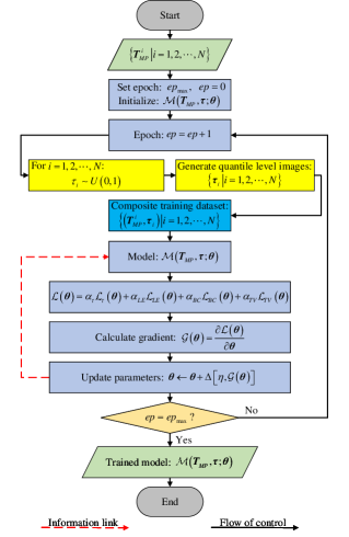
Figure 5: The training flowchart of MC iterative training algorithm

Based on $N$ discretized MP temperature images $\left\{\bm{T}^{i}_{MP}|i=1,2,\cdots,N\right\}$, the corresponding quantile level images $\left\{{{\bm{\tau}}_{i}}\left|i=1,2,\cdots,N\right.\right\}$ can be obtained by Eq.(12) for the $ep\text{th}$ ($ep=1,2,\cdots,ep_{max}$) epoch. For the quantile level image ${{\bm{\tau}}_{i}}$ corresponding to the $i\text{th}$ discretized MP temperature image, the quantile level ${\tau}_{i}$ is randomly sampled from the uniform distribution $U\left(0,1\right)$ in each model training epoch. The training dataset $\left\{\left(\bm{T}_{MP}^{i},{{\bm{\tau}}_{i}}\right)\left|i=1,2,\cdots,N\right.\right\}$ is composited using the discretized MP temperature images $\left\{\bm{T}^{i}_{MP}|i=1,2,\cdots,N\right\}$ and the quantile level images $\left\{{{\bm{\tau}}_{i}}\left|i=1,2,\cdots,N\right.\right\}$. Then, the parameters $\bm{\theta}$ of model $\mathcal{M}\left(\bm{T}_{MP},\bm{\tau};\bm{\theta}\right)$ are learned by minimizing the proposed physics-informed loss function $\mathcal{L}\left(\theta\right)$, i.e.,

$${\bm{\theta}}=\underset{\bm{\theta}}{\mathop{\arg}}\,\min\left[{\alpha}_{\tau}{{\mathcal{L}}_{\tau}}\left(\bm{\theta}\right)+{{\alpha}_{LE}}{{\mathcal{L}}_{LE}}\left(\bm{\theta}\right)+{{\alpha}_{BC}}{{\mathcal{L}}_{BC}}\left(\bm{\theta}\right)+{{\alpha}_{TV}}{{\mathcal{L}}_{TV}}\left(\bm{\theta}\right)\right].$$ (25)

The proposed MC iterative training algorithm uses the Adam algorithm [51] to iteratively solve Eq.(25). Based on the composited training dataset $\left\{\left(\bm{T}_{MP}^{i},{{\bm{\tau}}_{i}}\right)\left|i=1,2,\cdots,N\right.\right\}$, the proposed physics-informed loss function $\mathcal{L}\left(\bm{\theta}\right)$ is calculated by Eq.(24). Therefore, the gradient $\mathcal{G}\left(\bm{\theta}\right)$ is derived by the chain rule for differentiating compositions of functions using automatic differentiation [52], i.e.,

$$\mathcal{G}\left(\bm{\theta}\right)=\frac{\partial\mathcal{L}\left(\bm{\theta}\right)}{\partial\left(\bm{\theta}\right)}.$$ (26)

In the training process, the parameters $\bm{\theta}$ is updated iteratively as follows:

$$\bm{\theta}\leftarrow\bm{\theta}+\Delta\left[\eta,\mathcal{G}\left(\bm{\theta}\right)\right],$$ (27)

where $\eta$ is the learning rate, and $\Delta\left(\cdot\right)$ is the calculation update operator determined by the Adam algorithm [51]. In summary, the pseudo code for training the physics-informed Deep MC-QR model $\mathcal{M}\left(\bm{T}_{MP},\bm{\tau};\bm{\theta}\right)$ is shown in Algorithm 1. In particular, different from the existing DCNN training methods, the key step of the MC iterative training algorithm is that the quantile level images $\left\{{{\bm{\tau}}_{i}}\left|i=1,2,\cdots,N\right.\right\}$ are randomly generated by Eq.(12) in each training epoch.

Input:

  (1) Learning rate $\eta$;

  (2) Maximum training epoch $ep_{max}$;

  (3) Hyperparameters: ${\alpha}_{\tau}$, ${\alpha}_{LE}$, ${\alpha}_{BC}$, ${\alpha}_{TV}$;

  (4) $N$ discretized MP temperature images $\left\{\bm{T}^{i}_{MP}|i=1,2,\cdots,N\right\}$.

Output:

  Trained physics-informed Deep MC-QR model $\mathcal{M}\left(\bm{T}_{MP},\bm{\tau};\bm{\theta}\right)$.

1

2Initialize the physics-informed Deep MC-QR model $\mathcal{M}\left(\bm{T}_{MP},\bm{\tau};\bm{\theta}\right)$;

3 for $ep=1:ep_{max}$ do

4       for $i=1:N$ do

5             Randomly take a sample ${\tau}_{i}$ from uniform distribution $U\left(0,1\right)$;

6             Create a ${{H}_{\Omega}}\times{{W}_{\Omega}}$ two-dimensional array $\bm{\tau}_{i}$ with all zero elements;

7             Perform $\bm{\tau}_{i}\left(x,y\right)={\tau}_{i}$ for $\forall\left(x,y\right)\in{{\Omega}_{MP}}$;

8             Composite training data $\left(\bm{T}_{MP}^{i},{{\bm{\tau}}_{i}}\right)$;

9             Estimate the reconstructed temperature field ${{\hat{\bm{T}}}_{i}}=\mathcal{M}\left(\bm{T}^{i}_{MP},\bm{\tau}_{i};\bm{\theta}\right)$.

10       end for

11      Calculate the quantile MP temperature mean error $\mathcal{L}_{\tau}\left(\bm{\theta}\right)$;

12       Calculate the Laplace equation mean squared error $\mathcal{L}_{LE}\left(\bm{\theta}\right)$;

13       Calculate the boundary condition mean squared error $\mathcal{L}_{BC}\left(\bm{\theta}\right)$;

14       Calculate the TV regularization $\mathcal{L}_{TV}\left(\bm{\theta}\right)$;

15       Calculate the proposed physics-informed loss function $\mathcal{L}\left(\bm{\theta}\right)={\alpha}_{\tau}{{\mathcal{L}}_{\tau}}\left(\bm{\theta}\right)+{{\alpha}_{LE}}{{\mathcal{L}}_{LE}}\left(\bm{\theta}\right)+{{\alpha}_{BC}}{{\mathcal{L}}_{BC}}\left(\bm{\theta}\right)+{{\alpha}_{TV}}{{\mathcal{L}}_{TV}}\left(\bm{\theta}\right)$;

16       Calculate the gradient $\mathcal{G}\left(\bm{\theta}\right)$ of the cost function $\mathcal{J}\left(\bm{\theta}\right)$;

17       Calculate the calculation update operator $\Delta\left[\eta,\mathcal{G}\left(\bm{\theta}\right)\right]$;

18       Update the paramters $\bm{\theta}\leftarrow\bm{\theta}+\Delta\left[\eta,\mathcal{G}\left(\bm{\theta}\right)\right]$.

19 end for

Algorithm 1 Physics-informed Deep MC-QR model MC iterative training algorithm.

3.4 Satellite TFR and aleatoric uncertainty quantification algorithm

Refer to section 3.3, the trained physics-informed Deep MC-QR model $\mathcal{M}\left(\bm{T}_{MP},\bm{\tau};\bm{\theta}\right)$ can be obtained by the proposed MC iterative training algorithm. For the MP temperature image $\bm{T}^{pre}_{MP}$, $N_{pre}$ quantile levels $\left\{{\tau}_{\mathcal{P}}^{pre}|\mathcal{P}=1,2,\cdots,N_{pre}\right\}$ are sampled from uniform distribution $U\left(0,1\right)$. Then, $N_{pre}$ quantile level images $\left\{\bm{\tau}_{\mathcal{P}}^{pre}|\mathcal{P}=1,2,\cdots,N_{pre}\right\}$ are generated by Eq.(12), based on which the prediction dataset $\mathcal{D}_{pre}$, i.e.,

$$\mathcal{D}_{pre}=\left\{\left(\bm{T}^{pre}_{MP},\bm{\tau}_{\mathcal{P}}^{pre}\right)|\mathcal{P}=1,2,\cdots,N_{pre}\right\}$$ (28)

are composited for the MP temperature image $\bm{T}^{pre}_{MP}$. For $\mathcal{P}=1,2,\cdots,N_{pre}$, the temperature field $\hat{\bm{T}}_{\mathcal{P}}^{pre}$ is predicted by the trained physics-informed Deep MC-QR model $\mathcal{M}\left(\bm{T}_{MP},\bm{\tau};\bm{\theta}\right)$, i.e., $\hat{\bm{T}}_{\mathcal{P}}^{pre}=\mathcal{M}\left(\bm{T}^{pre}_{MP},\bm{\tau}_{\mathcal{P}}^{pre};\bm{\theta}\right)$. Thereby, the reconstructed temperature field’s approximation $\hat{\bm{T}}_{pre}$ is predicted by calculating the mean of $N_{pre}$ results $\hat{\bm{T}}_{\mathcal{P}}^{pre}$ ($\mathcal{P}=1,2,\cdots,N_{pre}$), i.e.,

$${{\hat{\bm{T}}}_{pre}}=\frac{1}{N_{pre}}\sum\limits_{\mathcal{P}=1}^{{{N}_{pre}}}{\hat{\bm{T}}_{\mathcal{P}}^{pre}}=\frac{1}{N_{pre}}\sum\limits_{\mathcal{P}=1}^{{{N}_{pre}}}{\mathcal{M}\left(\bm{T}_{MP}^{pre},\bm{\tau}_{\mathcal{P}}^{pre};\bm{\theta}\right)}.$$ (29)

Besides, the aleatoric uncertainty $\bm{\sigma}_{pre}$ of the reconstructed temperature field $\hat{\bm{T}}_{pre}$ can be quantified by calculating the standard deviation of $N_{pre}$ results $\hat{\bm{T}}_{\mathcal{P}}^{pre}$ ($\mathcal{P}=1,2,\cdots,N_{pre}$), i.e.,

$${{\bm{\sigma}}_{pre}}={{\left[\frac{1}{N_{pre}}\sum\limits_{\mathcal{P}=1}^{{{N}_{pre}}}{{{\left(\hat{\bm{T}}_{\mathcal{P}}^{pre}\right)}^{2}}-{{\left({{{\hat{\bm{T}}}}_{pre}}\right)}^{2}}}\right]}^{\frac{1}{2}}}$$ (30)

$$\quad\;\,\,\,={{\left\{\frac{1}{N_{pre}}{{\sum\limits_{\mathcal{P}=1}^{{{N}_{pre}}}{{{\left[\mathcal{M}\left(\bm{T}_{MP}^{pre},\bm{\tau}_{\mathcal{P}}^{pre};\bm{\theta}\right)\right]}^{2}}-\left[\frac{1}{N_{pre}}\sum\limits_{\mathcal{P}=1}^{{{N}_{pre}}}{\mathcal{M}\left(\bm{T}_{MP}^{pre},\bm{\tau}_{\mathcal{P}}^{pre};\bm{\theta}\right)}\right]}}^{2}}\right\}}^{\frac{1}{2}}}$$

$$\quad\;\,\,\,=\frac{1}{{{N}_{pre}^{2}}}{{\left\{{{\sum\limits_{\mathcal{P}=1}^{{{N}_{pre}}}{{{\left[\mathcal{M}\left(\bm{T}_{MP}^{pre},\bm{\tau}_{\mathcal{P}}^{pre};\bm{\theta}\right)\right]}^{2}}-\frac{1}{N_{pre}}\left[\sum\limits_{\mathcal{P}=1}^{{{N}_{pre}}}{\mathcal{M}\left(\bm{T}_{MP}^{pre},\bm{\tau}_{\mathcal{P}}^{pre};\bm{\theta}\right)}\right]}}^{2}}\right\}}^{\frac{1}{2}}}.$$

In summary, the pseudo code for predicting the reconstructed satellite subsystem temperature field and quantifying the aleatoric uncertainty is shown in the following Algorithm 2.

Input:

  (1) MP temperature image $\bm{T}^{pre}_{MP}$;

  (2) The number $N_{pre}$ of quantile levels;

  (3) Trained physics-informed Deep MC-QR model $\mathcal{M}\left(\bm{T}_{MP},\bm{\tau};\bm{\theta}\right)$.

Output:

  (1) Reconstructed satellite subsystem temperature field ${{\hat{\bm{T}}}_{pre}}$;

  (2) Quantified aleatoric uncertainty $\hat{\bm{\sigma}}_{pre}$.

1

2for $\mathcal{P}=1:N_{pre}$ do

3       Randomly take a sample ${\tau}^{pre}_{\mathcal{P}}$ from uniform distribution $U\left(0,1\right)$;

4       Create a ${{H}_{\Omega}}\times{{W}_{\Omega}}$ two-dimensional array $\bm{\tau}^{pre}_{\mathcal{P}}$ with all zero elements;

5       Perform $\bm{\tau}^{pre}_{\mathcal{P}}\left(x,y\right)={\tau}^{pre}_{\mathcal{P}}$ for $\forall\left(x,y\right)\in{{\Omega}_{MP}}$;

6       Composite training data $\left(\bm{T}^{pre}_{MP},\bm{\tau}^{pre}_{\mathcal{P}}\right)$;

7       Predict the reconstructed temperature field ${{\hat{\bm{T}}}^{pre}_{\mathcal{P}}}=\mathcal{M}\left(\bm{T}^{pre}_{MP},\bm{\tau}^{pre}_{\mathcal{P}};\bm{\theta}\right)$.

8 end for

9Calculate the mean ${{\hat{\bm{T}}}_{pre}}$ of $\left\{{{\hat{\bm{T}}}^{pre}_{\mathcal{P}}}|\mathcal{P}=1,2,\cdots,N_{pre}\right\}$ by Eq.(29);

10 Calculate the standard deviation $\hat{\bm{\sigma}}_{pre}$ of $\left\{{{\hat{\bm{\sigma}}}^{pre}_{\mathcal{P}}}|\mathcal{P}=1,2,\cdots,N_{pre}\right\}$ by Eq.(30).

Algorithm 2 Satellite TFR and aleatoric uncertainty quantification algorithm.

Given the test dataset $\left\{\left(\bm{T}^{pre}_{MP,t},\bm{T}_{test}^{t}\right)|t=1,2,\cdots,N_{test}\right\}$, the reconstructed temperature field’s approximations $\left\{\hat{\bm{T}}^{t}_{pre}|t=1,2,\cdots,N_{MCS}\right\}$ can be obtained by the Algorithm 2. In this paper, the prediction performance of the trained model $\mathcal{M}\left(\bm{T}_{MP},\bm{\tau};\bm{\theta}\right)$ is evaluated by the following four indicators, i.e.,

• the average of root mean square error (RMSE)

  $$\overline{RMSE}=\frac{1}{{{N}_{test}}}\sum\limits_{t=1}^{{{N}_{test}}}{\sqrt{\frac{1}{{{H}_{\Omega}}\times{{W}_{\Omega}}}\sum\limits_{\left(x,y\right)\in\Omega}{{{\left[\bm{T}_{test}^{t}\left(x,y\right)-\bm{\hat{T}}_{pre}^{t}\left(x,y\right)\right]}^{2}}}}},$$ (31)

• the average of mean absolute error (MAE)

  $$\overline{MAE}=\frac{1}{{{N}_{test}}}\sum\limits_{t=1}^{{{N}_{test}}}{\frac{1}{{{H}_{\Omega}}\times{{W}_{\Omega}}}\sum\limits_{\left(x,y\right)\in\Omega}{\left|\bm{T}_{test}^{t}\left(x,y\right)-\bm{\hat{T}}_{pre}^{t}\left(x,y\right)\right|}},$$ (32)

• the average of mean relative error (MRE)

  $$\overline{MRE}=\frac{1}{{{N}_{test}}}\sum\limits_{t=1}^{{{N}_{test}}}{\frac{1}{{{H}_{\Omega}}\times{{W}_{\Omega}}}\sum\limits_{\left(x,y\right)\in\Omega}{\frac{\left|\bm{T}_{test}^{t}\left(x,y\right)-\bm{\hat{T}}_{pre}^{t}\left(x,y\right)\right|}{\bm{T}_{test}^{t}\left(x,y\right)}}},$$ (33)

• the average of R square ($R^{2}$)

  $$\bm{\bar{T}}_{pre}^{t}=\frac{1}{{{N}_{test}}}\sum\limits_{t=1}^{{{N}_{test}}}{\bm{\hat{T}}_{pre}^{t}},$$ (34)

  $$\overline{{{R}^{2}}}=\frac{1}{{{N}_{test}}}\sum\limits_{t=1}^{{{N}_{test}}}{\left\{1-{\frac{\sum\limits_{\left(x,y\right)\in\Omega}{{\left[\bm{T}_{test}^{t}\left(x,y\right)-\bm{\hat{T}}_{pre}^{t}\left(x,y\right)\right]}^{2}}}{\sum\limits_{\left(x,y\right)\in\Omega}{{\left[\bm{T}_{test}^{t}\left(x,y\right)-\bm{\bar{T}}_{pre}^{t}\left(x,y\right)\right]}^{2}}}}\right\}}.$$

For the first three indicators $\overline{RMSE}$, $\overline{MAE}$ and $\overline{MRE}$, the closer their values are to 0, the higher the accuracy of the trained model $\mathcal{M}\left(\bm{T}_{MP},\bm{\tau};\bm{\theta}\right)$. For the average of R square, ${{R}^{2}}\to 1$ means that the trained model $\mathcal{M}\left(\bm{T}_{MP},\bm{\tau};\bm{\theta}\right)$ can estimate the reconstructed satellite subsystem temperature field accurately.

4 Satellite heat reliability analysis based on interval multilevel BN

4.1 Aleatoric uncertainty-based satellite component normal probability interval estimation

Due to the approximation $\hat{\bm{T}}_{pre}$ with the aleatoric uncertainty $\bm{\sigma}_{pre}$, the interval temperature field $\widetilde{\bm{T}}_{pre}$ is used to represent the reconstructed temperature field of the MP temperature image $\bm{T}^{pre}_{MP}$, i.e.,

$${{{\hat{\bm{T}}}}_{+}}={{{\hat{\bm{T}}}}_{pre}}+\lambda{{\bm{\sigma}}_{pre}},$$ (35)

$${{{\hat{\bm{T}}}}_{-}}={{{\hat{\bm{T}}}}_{pre}}-\lambda{{\bm{\sigma}}_{pre}},$$

$${{{\bm{\widetilde{T}}}}_{pre}}=\left[{{{\hat{\bm{T}}}}_{-}},{{{\hat{\bm{T}}}}_{+}}\right],$$

where $\lambda$ is the hyperparameter. In Eq.(35), any element in ${{{\hat{\bm{T}}}}_{+}}$ and ${{{\hat{\bm{T}}}}_{-}}$ is greater than or equal to zero, i.e., $\forall\left(x,y\right)\in{\Omega}$, ${{{\hat{\bm{T}}}}_{+}}\left(x,y\right)\geq 0$ and ${{{\hat{\bm{T}}}}_{-}}\left(x,y\right)\geq 0$. Define that ${\Omega}_{C_{s}}$ represents the area where the component $C_{s}$ ($s=1,2,\cdots,n$) is located in $\Omega$ (Fig.2(a)). The interval highest temperature $\widetilde{T}_{s}$ in the area ${\Omega}_{C_{s}}$ is

$${{\widetilde{T}}_{s}}=\left[\underset{\left(x,y\right)\in{{\Omega}_{{{C}_{s}}}}}{\mathop{\max}}\,{{{\hat{\bm{T}}}}_{-}}\left(x,y\right),\underset{\left(x,y\right)\in{{\Omega}_{{{C}_{s}}}}}{\mathop{\max}}\,{{{\hat{\bm{T}}}}_{+}}\left(x,y\right)\right].$$ (36)

The temperature field of the satellite subsystem will change with the different working power of the components, thereby affecting each component’s operating performance. In this paper, ${{C}_{s}}=0$ and ${{C}_{s}}=1$ indicate the component failure and normal, respectively. The working state of component $C_{s}$ depends on the interval highest temperature $T_{s}$ in the area ${\Omega}_{C_{s}}$, and the definitions of two working states are

$$\left\{\begin{aligned} &{{C}_{s}}=0,\qquad{{T}_{s}}\geq T_{lim}^{C_{s}}\\ &{{C}_{s}}=1,\qquad{{T}_{s}}<T_{lim}^{C_{s}}\\ \end{aligned}\right.,$$ (37)

where $T_{lim}^{C_{s}}$ is working state threshold for the component $C_{s}$.

Given $N_{MCS}$ MP temperature images $\left\{\bm{T}^{pre}_{MP,m}|m=1,2,\cdots,N_{MCS}\right\}$, the reconstructed temperature field’s approximations $\left\{\hat{\bm{T}}^{m}_{pre}|m=1,2,\cdots,N_{MCS}\right\}$ and the aleatoric uncertainty $\left\{\bm{\sigma}^{m}_{pre}|m=1,2,\cdots,N_{MCS}\right\}$ are obtained by Eqs.(29) and (30). Then, $N_{MCS}$ interval highest temperatures $\left\{\widetilde{T}^{m}_{s}|m=1,2,\cdots,N_{MCS}\right\}$ are calculated using Eqs.(35) and (36). Thus, the interval highest temperatures’ lower bound set ${\mathcal{T}}^{lower}_{s}$ and upper bound set ${\mathcal{T}}^{upper}_{s}$ respectively are

$${\mathcal{T}}^{lower}_{s}=\left\{\widetilde{T}^{-m}_{s}|m=1,2,\cdots,N_{MCS}\right\},$$ (38)

$${\mathcal{T}}^{upper}_{s}=\left\{\widetilde{T}^{+m}_{s}|m=1,2,\cdots,N_{MCS}\right\},$$

where $\widetilde{T}^{-m}_{s}$ and $\widetilde{T}^{+m}_{s}$ are the lower bound and the upper bound of interval highest temperature $\widetilde{T}^{m}_{s}$, respectively. This section defines a set ${\mathcal{T}}^{\forall}_{s}$, i.e.,

$${\mathcal{T}}^{\forall}_{s}=\left\{T^{m}_{s}|T^{m}_{s}\in{{\widetilde{T}}^{m}_{s}},m=1,2,\cdots,N_{MCS}\right\},$$ (39)

where the set ${\mathcal{T}}^{\forall}_{s}$ satisfies two conditions ${\mathcal{T}}^{\forall}_{s}\neq{\mathcal{T}}^{lower}_{s}$ and ${\mathcal{T}}^{\forall}_{s}\neq{\mathcal{T}}^{upper}_{s}$. Suppose that ${{N}^{-}_{{{C}_{s}}=1}}$, ${{N}^{+}_{{{C}_{s}}=1}}$ and ${{N}^{\forall}_{{{C}_{s}}=1}}$ represent the number of elements satisfying the conditions $\widetilde{T}^{-m}<T_{lim}^{C_{s}}$, $\widetilde{T}^{+m}<T_{lim}^{C_{s}}$ and $T^{m}_{s}<T_{lim}^{C_{s}}$, respectively. Apparently, there is an inequality relationship

$${{N}^{+}_{{{C}_{s}}=1}}\leq{{N}^{\forall}_{{{C}_{s}}=1}}\leq{{N}^{-}_{{{C}_{s}}=1}}.$$ (40)

According to Eq.(37), three normal probabilities ${\Pr}^{-}\left({{C}_{s}}=1\right)$, ${\Pr}^{+}\left({{C}_{s}}=1\right)$ and ${\Pr}^{\forall}\left({{C}_{s}}=1\right)$ are

$${\Pr}^{-}\left({{C}_{s}}=1\right)=\frac{{{N}^{+}_{{{C}_{s}}=1}}}{{{N}_{MCS}}},$$ (41)

$${\Pr}^{+}\left({{C}_{s}}=1\right)=\frac{{{N}^{-}_{{{C}_{s}}=1}}}{{{N}_{MCS}}},$$

$${\Pr}^{\forall}\left({{C}_{s}}=1\right)=\frac{{{N}^{\forall}_{{{C}_{s}}=1}}}{{{N}_{MCS}}},$$

Refer to Eq.(40), three normal probabilities ${\Pr}^{-}\left({{C}_{s}}=1\right)$, ${\Pr}^{+}\left({{C}_{s}}=1\right)$ and ${\Pr}^{\forall}\left({{C}_{s}}=1\right)$ exist an inequality relation

$${\Pr}^{-}\left({{C}_{s}}=1\right)\leq{\Pr}^{\forall}\left({{C}_{s}}=1\right)\leq{\Pr}^{+}\left({{C}_{s}}=1\right).$$ (42)

Therefore, the normal probability interval $\widetilde{\Pr}\left({{C}_{s}}=1\right)$ is

$$\widetilde{\Pr}\left({{C}_{s}}=1\right)=\left[{\Pr}^{-}\left({{C}_{s}}=1\right),{\Pr}^{+}\left({{C}_{s}}=1\right)\right].$$ (43)

In summary, the pseudo code for calculating the satellite component normal probability interval is shown in the following Algorithm 3.

Input:

  (1) Hyperparameter $\lambda$;

  (2) Working state thresholds $\left\{T_{lim}^{C_{s}}|s=1,2,\cdots,n\right\}$ ;

  (3) The number $N_{pre}$ of quantile levels;

  (4) Trained physics-informed Deep MC-QR model $\mathcal{M}\left(\bm{T}_{MP},\bm{\tau};\bm{\theta}\right)$;

  (5) $N_{MCS}$ discretized MP temperature images $\left\{\bm{T}^{pre}_{MP,m}|m=1,2,\cdots,N_{MCS}\right\}$.

Output:

  Satellite component normal probability interval $\left\{\widetilde{\Pr}\left({{C}_{s}=1}\right)|s=1,2,\cdots,n\right\}$.

1

2for $m=1:N_{MCS}$ do

3       Calculate the mean ${{\hat{\bm{T}}}^{m}_{pre}}$ and the standard deviation $\hat{\bm{\sigma}}^{m}_{pre}$ by the Algorithm 2;

4       Calculate the interval highest temperatures $\widetilde{T}^{m}_{s}$ by Eqs.(35) and (36).

5      

6 end for

7for $s=1:n$ do

8       Construct the lower bound set ${\mathcal{T}}^{lower}_{s}=\left\{\widetilde{T}^{-m}_{s}|m=1,2,\cdots,N_{MCS}\right\}$;

9       Construct the upper bound set ${\mathcal{T}}^{upper}_{s}=\left\{\widetilde{T}^{+m}_{s}|m=1,2,\cdots,N_{MCS}\right\}$;

10       Count the number ${{N}^{-}_{{{C}_{s}}=1}}$ of elements in the set ${\mathcal{T}}^{lower}_{s}$ that meet condition $\widetilde{T}^{-m}<T_{lim}^{C_{s}}$;

11       Count the number ${{N}^{+}_{{{C}_{s}}=1}}$ of elements in the set ${\mathcal{T}}^{lower}_{s}$ that meet condition $\widetilde{T}^{+m}<T_{lim}^{C_{s}}$;

12       Calculate the normal probability interval $\widetilde{\Pr}\left({{C}_{s}}=1\right)=\left[{\Pr}^{-}\left({{C}_{s}}=1\right),{\Pr}^{+}\left({{C}_{s}}=1\right)\right]$.

13 end for

Algorithm 3 Satellite component normal probability interval estimation algorithm.

4.2 Interval multilevel BN modeling for satellite heat reliability analysis

As shown in Fig.6, the components of the studied satellite subsystem $S$ in Fig.2(a) can be divided into $\stackrel{{\scriptstyle\frown}}{{m}}$ blocks $\left\{\mathcal{B}_{\stackrel{{\scriptstyle\frown}}{{i}}}|\stackrel{{\scriptstyle\frown}}{{i}}=1,2,\cdots,\stackrel{{\scriptstyle\frown}}{{m}}\right\}$. In Fig.6, ${{\Psi}_{S}}$ denotes the logical relationship between subsystem $S$ and $\stackrel{{\scriptstyle\frown}}{{m}}$ blocks, and ${{\Psi}_{\mathcal{B}_{\stackrel{{\scriptstyle\frown}}{{i}}}}}$ represents the logical relationship between the block $\mathcal{B}_{\stackrel{{\scriptstyle\frown}}{{i}}}$ and its $\stackrel{{\scriptstyle\frown}}{{n}}$ components. For the studied satellite subsystem $S$, the logical relationshipships between components mainly include series and parallel. Thus, the block $\mathcal{B}_{\stackrel{{\scriptstyle\frown}}{{i}}}$ may be series block $\mathcal{B}_{se}$ or parallel block $\mathcal{B}_{pa}$ as shown in Fig.6. Then, the blocks $\left\{\mathcal{B}_{\stackrel{{\scriptstyle\frown}}{{i}}}|\stackrel{{\scriptstyle\frown}}{{i}}=1,2,\cdots,\stackrel{{\scriptstyle\frown}}{{m}}\right\}$ are connected in series or parallel to form the satellite subsystem $S$, i.e. the logical relationship ${{\Psi}_{S}}$ may be series or parallel.

Figure 6: The studied satellite subsystem $S$. The block $\mathcal{B}_{\stackrel{{\scriptstyle\frown}}{{i}}}$ may be series block $\mathcal{B}_{se}$ and parallel block $\mathcal{B}_{pa}$ .

According to Fig.6, this section constructs a interval multilevel BN for analyzing the satellite subsystem $S$ reliability as shown in Fig.7. For the conditional probability table (CPT) of each non-root node, all parent nodes’ state combinations are determined by the format in [3, 4]. For example, the CPT $\Pr\left(S|{\mathcal{B}_{1}},{\mathcal{B}_{2}},\cdots,{\mathcal{B}_{\stackrel{{\scriptstyle\frown}}{{m}}}}\right)$ of the leaf node $S$ is shown in Table 1, where $S=0$ and $S=1$ respectively denote the subsystem failure and normal, the values of variables $\left\{p_{1,1},p_{1,2},\cdots,p_{2^{n},1}p_{2^{n},2}\right\}$ are determined by the logical relationship ${{\Psi}_{S}}$. By the variable elimination algorithm (VE) [53], the interval probability distribution $\widetilde{\Pr}\left(S\right)$ of the child node $S$ can be calculated by Eq.(44).

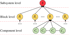
Figure 7: An interval multilevel BN for analyzing the heat reliability of the satellite subsystem

Table 1: The CPT $\Pr\left(S|{\mathcal{B}_{1}},{\mathcal{B}_{2}},\cdots,{\mathcal{B}_{\stackrel{{\scriptstyle\frown}}{{m}}}}\right)$ of the leaf node $S$

$\mathcal{B}_{1}$	$\mathcal{B}_{2}$	$\cdots$	${\mathcal{B}_{\stackrel{{\scriptstyle\frown}}{{m}}-1}}$	$\mathcal{B}_{\stackrel{{\scriptstyle\frown}}{{m}}}$	$\Pr\left(S|{\mathcal{B}_{1}},{\mathcal{B}_{2}},\cdots,{\mathcal{B}_{\stackrel{{\scriptstyle\frown}}{{m}}}}\right)$
					$S=0$	$S=1$
0	0	$\cdots$	0	0	$p_{1,1}$	$p_{1,2}$
0	0	$\cdots$	0	1	$p_{2,1}$	$p_{2,2}$
0	0	$\cdots$	1	0	$p_{3,1}$	$p_{3,2}$
0	0	$\cdots$	1	1	$p_{4,1}$	$p_{4,2}$
$\vdots$	$\vdots$	$\vdots$	$\vdots$	$\vdots$	$\vdots$	$\vdots$
1	1	$\cdots$	0	0	$p_{(2^{\stackrel{{\scriptstyle\frown}}{{m}}}-3),1}$	$p_{(2^{\stackrel{{\scriptstyle\frown}}{{m}}}-3),2}$
1	1	$\cdots$	0	1	$p_{(2^{\stackrel{{\scriptstyle\frown}}{{m}}}-2),1}$	$p_{(2^{\stackrel{{\scriptstyle\frown}}{{m}}}-2),2}$
1	1	$\cdots$	1	0	$p_{(2^{\stackrel{{\scriptstyle\frown}}{{m}}}-1),1}$	$p_{(2^{\stackrel{{\scriptstyle\frown}}{{m}}}-1),2}$
1	1	$\cdots$	1	1	$p_{2^{\stackrel{{\scriptstyle\frown}}{{m}}},1}$	$p_{2^{\stackrel{{\scriptstyle\frown}}{{m}}},2}$

$${\widetilde{\Pr}}\left(S\right)=\sum\limits_{\mathcal{B}_{1}}^{2}{\cdots\sum\limits_{{\mathcal{B}_{\stackrel{{\scriptstyle\frown}}{{m}}-1}}=1}^{2}{\sum\limits_{\mathcal{B}_{\stackrel{{\scriptstyle\frown}}{{m}}}=1}^{2}{{\widetilde{\Pr}}\left({\mathcal{B}_{1}},{\mathcal{B}_{2}},\cdots,{\mathcal{B}_{\stackrel{{\scriptstyle\frown}}{{m}}}},S\right)}}}$$ (44)

$$\qquad\;\;\,=\sum\limits_{{\mathcal{B}_{1}}=1}^{2}{\cdots\sum\limits_{{\mathcal{B}_{\stackrel{{\scriptstyle\frown}}{{m}}-1}}=1}^{2}{\sum\limits_{\mathcal{B}_{\stackrel{{\scriptstyle\frown}}{{m}}}=1}^{2}{{\widetilde{\Pr}}\left({\mathcal{B}_{1}}\right)\cdots{\widetilde{\Pr}}\left({\mathcal{B}_{\stackrel{{\scriptstyle\frown}}{{m}}-1}}\right){\widetilde{\Pr}}\left({\mathcal{B}_{\stackrel{{\scriptstyle\frown}}{{m}}}}\right)\Pr\left(S|{\mathcal{B}_{1}},{\mathcal{B}_{2}},\cdots,{\mathcal{B}_{\stackrel{{\scriptstyle\frown}}{{m}}}}\right)}}}$$

$$\qquad\;\;\,=\sum\limits_{\mathcal{B}_{1}=1}^{2}{{\widetilde{\Pr}}\left({\mathcal{B}_{1}}\right)\cdots\sum\limits_{{\mathcal{B}_{\stackrel{{\scriptstyle\frown}}{{m}}-1}}=1}^{2}{{\widetilde{\Pr}}\left({\mathcal{B}_{\stackrel{{\scriptstyle\frown}}{{m}}-1}}\right)\sum\limits_{\mathcal{B}_{\stackrel{{\scriptstyle\frown}}{{m}}}=1}^{2}{{\widetilde{\Pr}}\left({\mathcal{B}_{\stackrel{{\scriptstyle\frown}}{{m}}}}\right)\Pr\left(S|{\mathcal{B}_{1}},{\mathcal{B}_{2}},\cdots,{\mathcal{B}_{\stackrel{{\scriptstyle\frown}}{{m}}}}\right)}}}$$

For $\stackrel{{\scriptstyle\frown}}{{i}}=1,2,\cdots,\stackrel{{\scriptstyle\frown}}{{m}}$, the interval probability ${\widetilde{\Pr}}\left({\mathcal{B}_{\stackrel{{\scriptstyle\frown}}{{i}}}}\right)$ in Eq.(44) is calculated by

$${\widetilde{\Pr}}\left({\mathcal{B}_{\stackrel{{\scriptstyle\frown}}{{i}}}}\right)=\widetilde{\Pr}\left({{\mathcal{B}}_{se}}\right)$$ (45)

for series logical relationship or calculated by

$${\widetilde{\Pr}}\left({\mathcal{B}_{\stackrel{{\scriptstyle\frown}}{{i}}}}\right)=\widetilde{\Pr}\left({{\mathcal{B}}_{pa}}\right)$$ (46)

for parallel logical relationship, where $\widetilde{\Pr}\left({{\mathcal{B}}_{se}}\right)$ and $\widetilde{\Pr}\left({{\mathcal{B}}_{pa}}\right)$ are calculated as follows.

For the series block $\mathcal{B}_{se}$ in Fig.6, its normal probability interval $\widetilde{\Pr}\left(\mathcal{B}_{se}=1\right)$ is

$$\widetilde{\Pr}\left({{\mathcal{B}}_{se}}=1\right)=\prod\limits_{\mathcal{K}=1}^{\stackrel{{\scriptstyle\frown}}{{n}}}{\widetilde{\Pr}\left({{C}_{\mathcal{K}}}=1\right)}.$$ (47)

For the parallel block $\mathcal{B}_{pa}$ in Fig.6, its normal probability interval $\widetilde{\Pr}\left({{\mathcal{B}}_{pa}}=1\right)$ (See the A for the detailed derivation process.) is

$$\widetilde{\Pr}\left({{\mathcal{B}}_{pa}}=1\right)=1-\prod\limits_{{\mathcal{K}}=1}^{\stackrel{{\scriptstyle\frown}}{{n}}}{\left[1-\widetilde{\Pr}\left({{C}_{\mathcal{K}}}=1\right)\right]}.$$ (48)

Like the calculations of $\widetilde{\Pr}\left({{\mathcal{B}}_{se}}\right)$ and $\widetilde{\Pr}\left({{\mathcal{B}}_{pa}}\right)$, the interval probability $\widetilde{\Pr}\left(S=1\right)$ can be calculated based on Eqs.(44), (47), and (48).

5 Case study

In this section, two case studies are used for verifying the effectiveness of the proposed methods. Two U-nets in the physics-informed Deep MC-QR method are modeled by PyTorch. The first case study is used to validate that the proposed physics-informed Deep MC-QR method can accurately reconstruct the temperature field and precisely quantify the aleatoric uncertainty caused by data noise. The second case study analyzes the heat reliability of a satellite subsystem. For two case studies, the hyperparameters ${\alpha}_{\tau}$, ${\alpha}_{LE}$, ${\alpha}_{BC}$, and ${\alpha}_{TV}$ are equal to $1\times 10^{5}$, $1\times 10^{2}$, $1\times 10^{2}$ and $1\times 10^{4}$, respectively. The relevant codes of the physics-informed Deep MC-QR method by Python are available on this website. In this paper, the unit of temperature is K. In order to facilitate training model, the MP temperature value is normalized by ${(\bm{T}_{MP}-298)}/{50}\;$. In the prediction, the parameter $N_{pre}$ is 200 for two cases.

5.1 Case 1: Physics-informed Deep MC-QR method validation

The first case uses a hypothetical subsystem with 19 components, as shown in Fig.8. The length $L$ is equal to 0.1m, and the width $\delta$ of the heat sink is 0.01m. The probability distributions of all component powers are shown in Table 2. This case uses 280 sensors to monitor the point temperature, where the positions of all sensors are shown in Fig.8.

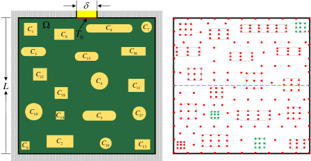
Figure 8: A hypothetical subsystem with 19 components in case 1.

Table 2: All component powers’ probability distributions in case 1.

Component	Mean	Standard deviation	Distribution
$C_{1}$	30000	6000	Gumbel
$C_{2}$	38900	9092	Lognormal
$C_{3}$	35000	5000	Normal
$C_{4}$	41200	9140	Gumbel
$C_{5}$	36000	8024	Lognormal
$C_{6}$	12000	1590	Normal
$C_{8}$	31200	7150	Gumbel
$C_{9}$	40000	5521	Normal
$C_{11}$	31000	4311	Normal
$C_{12}$	28070	6100	Lognormal
$C_{13}$	29800	4321	Normal
$C_{16}$	28900	7216	Gumbel
$C_{17}$	22100	5021	Lognormal
$C_{18}$	22000	2521	Normal
Component	Lower boundary	Upper boundary	Distribution
$C_{7}$	100	12000	Uniform
$C_{10}$	2000	30000	Uniform
$C_{14}$	0	10000	Uniform
$C_{15}$	500	28000	Uniform
$C_{19}$	100	13000	Uniform

5.1.1 Preparing monitoring point temperature data

In this paper, the two-dimensional square area $\Omega$ is divided into a $200\times 200$ grid $\bm{G}$. The values of grid cells in the area ${\Omega}_{C_{s}}$ ($s=1,2,\cdots,19$) are equal to the power $P_{s}$ of the component $C_{s}$, and the values of grid cells in the area ${\Omega}_{NC}$ are equal to zero. According to the component powers’ distributions, 20000 grids $\left\{\bm{G}_{1},\bm{G}_{2},\cdots,\bm{G}_{20000}\right\}$ are sampled by the Latin Hypercube Sampling. Then, 20000 temperature fields $\left\{{\bm{T}}_{1},{\bm{T}}_{2},\cdots,{\bm{T}}_{20000}\right\}$ are generated by the recon-data-generator. Refer to all sensors’ positions, their values are taken from the temperature fields $\left\{{\bm{T}}_{1},{\bm{T}}_{2},\cdots,{\bm{T}}_{20000}\right\}$ to form 20000 MP temperatures $\left\{\bm{T}^{1}_{MP},\bm{T}^{2}_{MP},\cdots,\bm{T}^{20000}_{MP}\right\}$. Based on these MP temperatures, this case prepares three kinds of datasets with Gaussian noises, i.e., $\mathcal{D}_{\varepsilon_{1}}$, $\mathcal{D}_{\varepsilon_{2}}$, and $\mathcal{D}^{b}_{\varepsilon_{1}}$, to validate that the proposed physics-informed Deep MC-QR method can accurately quantify the aleatoric uncertainty caused by data noise. The Gaussian noises ${\varepsilon}_{1}\sim N\left(0,{0.25}^{2}\right)$ and ${\varepsilon}_{2}\sim N\left(0,{0.50}^{2}\right)$ are added to the temperature sensors values of green points in Fig.8 to generate the first two datasets $\mathcal{D}_{\varepsilon_{1}}$ and $\mathcal{D}_{\varepsilon_{2}}$, respectively. The Gaussian noise ${\varepsilon}_{1}\sim N\left(0,{0.25}^{2}\right)$ is added to the temperature values of the measuring points below the blue line in Fig.8 to generate the last dataset $\mathcal{D}^{b}_{\varepsilon_{1}}$, respectively. For 20000 MP temperatures $\left\{\bm{T}^{1}_{MP},\bm{T}^{2}_{MP},\cdots,\bm{\textsc{T}}^{20000}_{MP}\right\}$, 10800 MP temperatures are used to train the physics-informed Deep MC-QR model $\mathcal{M}\left(\bm{T}_{MP},\bm{\tau};\bm{\theta}\right)$, 1200 MP temperatures are used to be the validate data, and the remaining 8000 MP temperatures are used to test the trained model $\mathcal{M}\left(\bm{T}_{MP},\bm{\tau};\bm{\theta}\right)$.

5.1.2 Result analysis

Model accuracy analysis

In this case, the maximum training epoch and the learning rate are set to be 400 and 0.1, respectively. Based on the prepared three kinds of training datasets, three models $\mathcal{M}^{{\varepsilon}_{1}}\left(\bm{T}_{MP},\bm{\tau};\bm{\theta}\right)$, $\mathcal{M}^{{\varepsilon}_{2}}\left(\bm{T}_{MP},\bm{\tau};\bm{\theta}\right)$ and $\mathcal{M}^{b{\varepsilon}_{1}}\left(\bm{T}_{MP},\bm{\tau};\bm{\theta}\right)$ are trained by the Algorithm 1. Then, the temperature fields corresponding for 8000 MP temperatures are reconstructed by the Algorithm 2. According to four indicators in section 3.4, the prediction performance of three trained models $\mathcal{M}^{{\varepsilon}_{1}}\left(\bm{T}_{MP},\bm{\tau};\bm{\theta}\right)$, $\mathcal{M}^{{\varepsilon}_{2}}\left(\bm{T}_{MP},\bm{\tau};\bm{\theta}\right)$ and $\mathcal{M}^{b{\varepsilon}_{1}}\left(\bm{T}_{MP},\bm{\tau};\bm{\theta}\right)$ are shown in Table 3. For three trained models, all three kinds of average errors, i.e., $\overline{RMSE}$, $\overline{MAE}$ and $\overline{MRE}$, are sufficiently small. Besides, the $\overline{R^{2}}$ values of three trained models are almost close to 1. Therefore, the proposed physics-informed Deep MC-QR method can construct an accurate surrogate model to reconstruct the temperature fields of the hypothetical subsystem.

Table 3: The prediction performance of three trained models $\mathcal{M}^{{\varepsilon}_{1}}\left(\bm{T}_{MP},\bm{\tau};\bm{\theta}\right)$, $\mathcal{M}^{{\varepsilon}_{2}}\left(\bm{T}_{MP},\bm{\tau};\bm{\theta}\right)$ and $\mathcal{M}^{b{\varepsilon}_{1}}\left(\bm{T}_{MP},\bm{\tau};\bm{\theta}\right)$ in case 1.

Dataset	Noise variance	Model	$\overline{RMSE}$	$\overline{MAE}$	$\overline{MRE}$	$\overline{R^{2}}$
$\mathcal{D}_{\varepsilon_{1}}$	$0.25^{2}$	$\mathcal{M}^{{\varepsilon}_{1}}\left(\bm{T}_{MP},\bm{\tau};\bm{\theta}\right)$	0.0511	0.0324	0.00009	0.9999
$\mathcal{D}_{\varepsilon_{2}}$	$0.50^{2}$	$\mathcal{M}^{{\varepsilon}_{2}}\left(\bm{T}_{MP},\bm{\tau};\bm{\theta}\right)$	0.0490	0.0306	0.00009	0.9999
$\mathcal{D}^{b}_{\varepsilon_{1}}$	$0.25^{2}$	$\mathcal{M}^{b{\varepsilon}_{1}}\left(\bm{T}_{MP},\bm{\tau};\bm{\theta}\right)$	0.0688	0.0486	0.00014	0.9999

As shown in Fig.9, this case randomly chooses four MP temperatures $\left\{\bm{T}^{1*}_{MP},\bm{T}^{2*}_{MP},\bm{T}^{3*}_{MP},\bm{T}^{4*}_{MP}\right\}$ to show the prediction effectiveness of three trained models $\mathcal{M}^{{\varepsilon}_{1}}\left(\bm{T}_{MP},\bm{\tau};\bm{\theta}\right)$, $\mathcal{M}^{{\varepsilon}_{2}}\left(\bm{T}_{MP},\bm{\tau};\bm{\theta}\right)$ and $\mathcal{M}^{b{\varepsilon}_{1}}\left(\bm{T}_{MP},\bm{\tau};\bm{\theta}\right)$. For four MP temperatures $\left\{\bm{T}^{1*}_{MP},\bm{T}^{2*}_{MP},\bm{T}^{3*}_{MP},\bm{T}^{4*}_{MP}\right\}$, their truth temperature fields $\left\{\bm{T}_{1*},\bm{T}_{2*},\bm{T}_{3*},\bm{T}_{4*}\right\}$ and reconstructed temperature fields by three trained models are presented in Fig.10. For each row, the last three reconstructed temperature fields are basically consistent with the first truth temperature field.

(a) MP temperature $\bm{T}^{1*}_{MP}$

(b) MP temperature $\bm{T}^{2*}_{MP}$

(c) MP temperature $\bm{T}^{3*}_{MP}$

(d) MP temperature $\bm{T}^{4*}_{MP}$

Figure 9: Four MP temperatures $\left\{\bm{T}^{1*}_{MP},\bm{T}^{2*}_{MP},\bm{T}^{3*}_{MP},\bm{T}^{4*}_{MP}\right\}$.

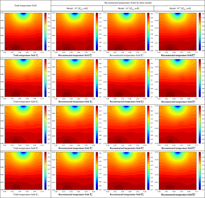
Figure 10: Four MP temperatures $\left\{\bm{T}^{1*}_{MP},\bm{T}^{2*}_{MP},\bm{T}^{3*}_{MP},\bm{T}^{4*}_{MP}\right\}$ and their truth temperature fields $\left\{\bm{T}_{1*},\bm{T}_{2*},\bm{T}_{3*},\bm{T}_{4*}\right\}$. The first column on the left is the truth temperature fields corresponding to four MP temperatures $\left\{\bm{T}^{1*}_{MP},\bm{T}^{2*}_{MP},\bm{T}^{3*}_{MP},\bm{T}^{4*}_{MP}\right\}$. For each row, the last three figures show the temperature fields reconstructed by the three models $\mathcal{M}^{{\varepsilon}_{1}}\left(\bm{T}_{MP},\bm{\tau};\bm{\theta}\right)$, $\mathcal{M}^{{\varepsilon}_{2}}\left(\bm{T}_{MP},\bm{\tau};\bm{\theta}\right)$ and $\mathcal{M}^{b{\varepsilon}_{1}}\left(\bm{T}_{MP},\bm{\tau};\bm{\theta}\right)$ for the same MP temperature.

Aleatoric uncertainty quantification result analysis

For four MP temperatures $\left\{\bm{T}^{1*}_{MP},\bm{T}^{2*}_{MP},\bm{T}^{3*}_{MP},\bm{T}^{4*}_{MP}\right\}$ (Fig.9) with two kinds of Gaussian noises ${\varepsilon}_{1}\sim N\left(0,{0.25}^{2}\right)$ and ${\varepsilon}_{2}\sim N\left(0,{0.50}^{2}\right)$, the corresponding aleatoric uncertainties are quantified based on the models $\mathcal{M}^{{\varepsilon}_{1}}\left(\bm{T}_{MP},\bm{\tau};\bm{\theta}\right)$ and $\mathcal{M}^{{\varepsilon}_{2}}\left(\bm{T}_{MP},\bm{\tau};\bm{\theta}\right)$ as shown in Figs.11 and 12, respectively. According to section 5.1.1, the models $\mathcal{M}^{{\varepsilon}_{1}}\left(\bm{T}_{MP},\bm{\tau};\bm{\theta}\right)$ and $\mathcal{M}^{{\varepsilon}_{2}}\left(\bm{T}_{MP},\bm{\tau};\bm{\theta}\right)$ are trained by the datasets that include the Gaussian noises (${\varepsilon}_{1}\sim N\left(0,{0.25}^{2}\right)$, ${\varepsilon}_{2}\sim N\left(0,{0.50}^{2}\right)$) in the green points in Fig.8. Refer to Figs.11 and 12, the aleatoric uncertainties corresponding to the areas of the green points are much larger than the other areas. For the magnitudes of aleatoric uncertainties in Figs.11 and 12, the maximum values are approximately equal to 0.25 ($\mathcal{M}^{{\varepsilon}_{1}}\left(\bm{T}_{MP},\bm{\tau};\bm{\theta}\right)$) and 0.5 ($\mathcal{M}^{{\varepsilon}_{2}}\left(\bm{T}_{MP},\bm{\tau};\bm{\theta}\right)$), respectively. Apparently, the magnitudes of two aleatoric uncertainties are basically the same as the magnitudes of two Gaussian noises. Therefore, the proposed physics-informed Deep MC-QR method can quantify the aleatoric uncertainty accurately.

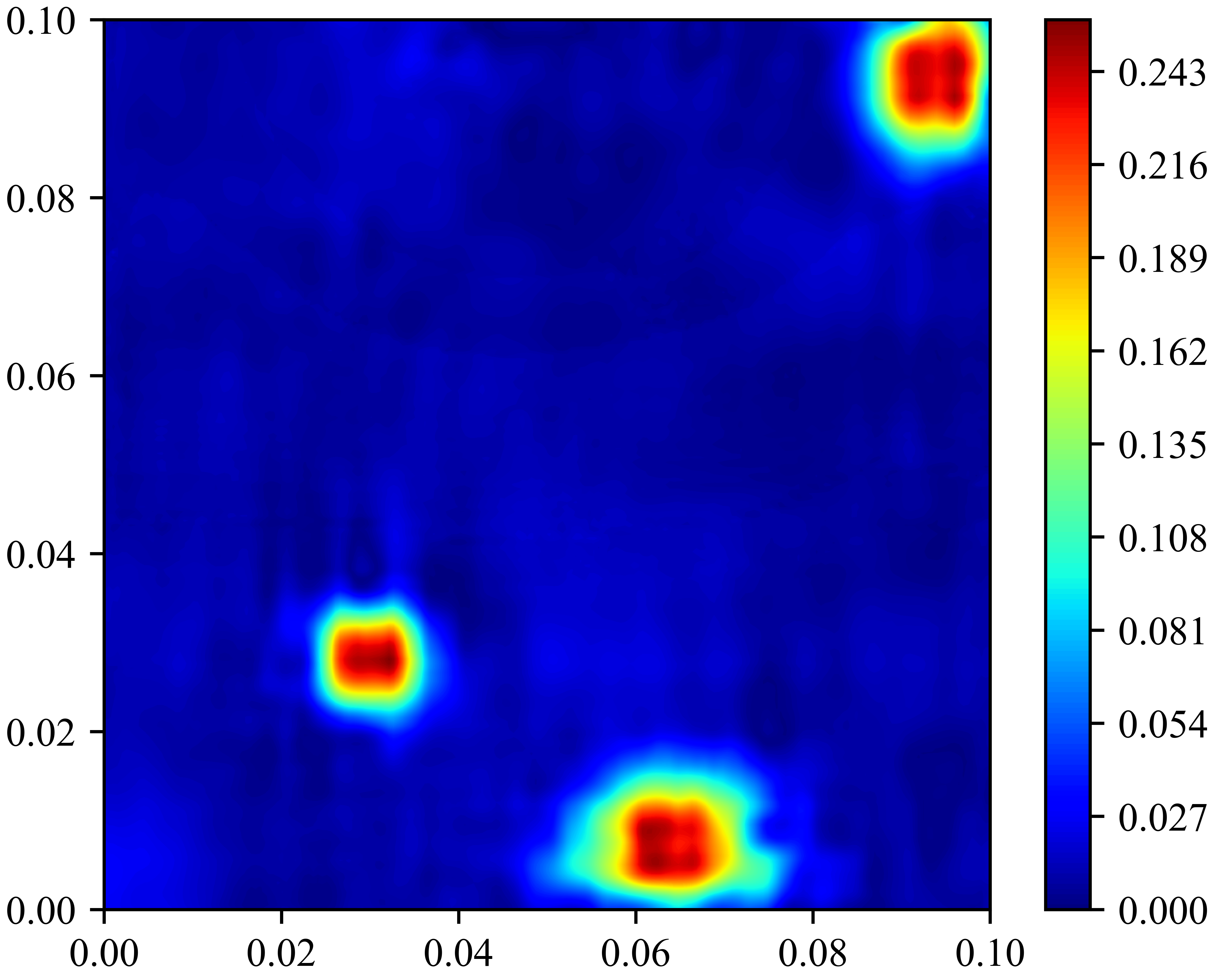
(a) Aleatoric uncertainty $\sigma_{1}^{{\varepsilon}_{1}}$

(b) Aleatoric uncertainty $\sigma_{2}^{{\varepsilon}_{1}}$

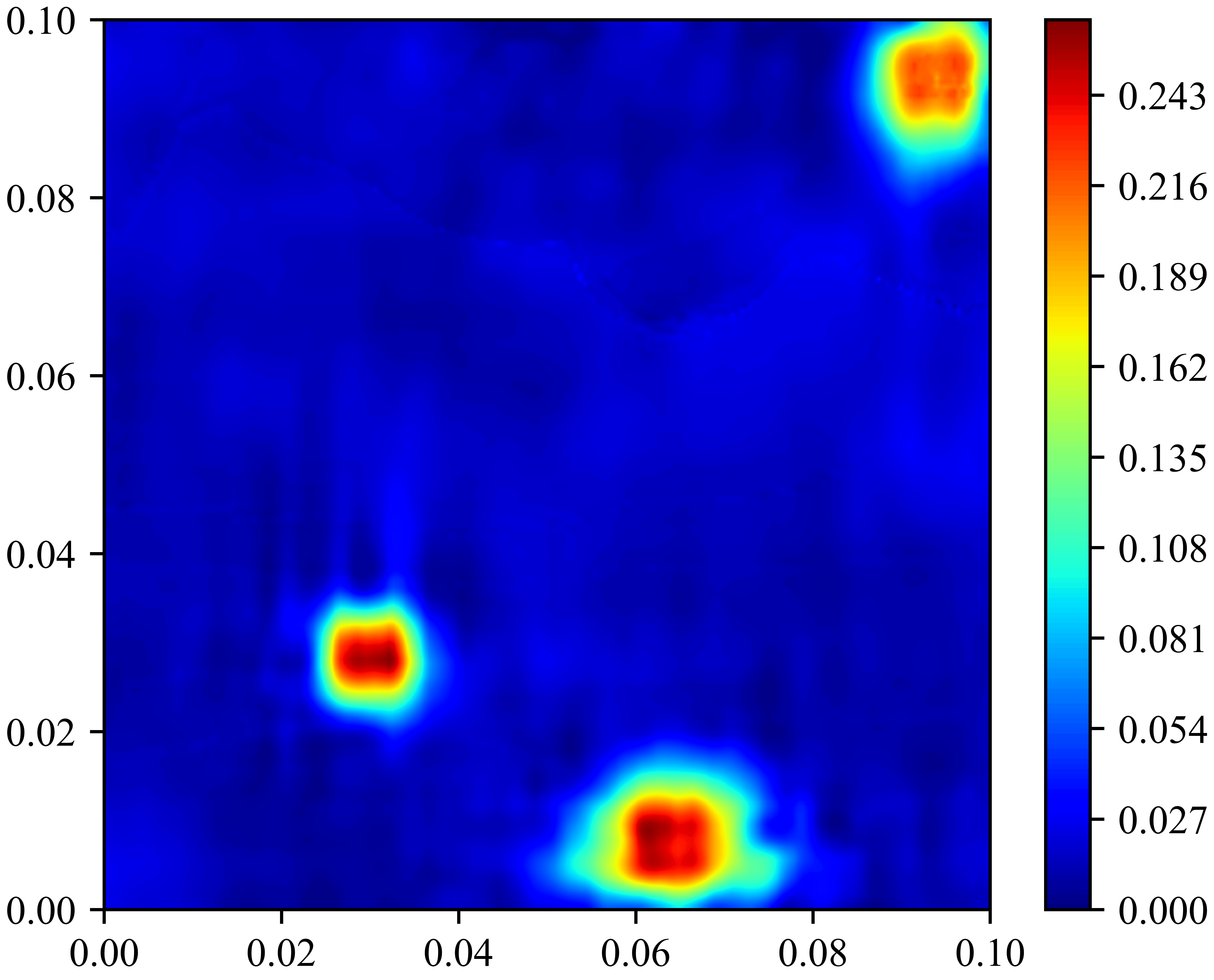
(c) Aleatoric uncertainty $\sigma_{3}^{{\varepsilon}_{1}}$

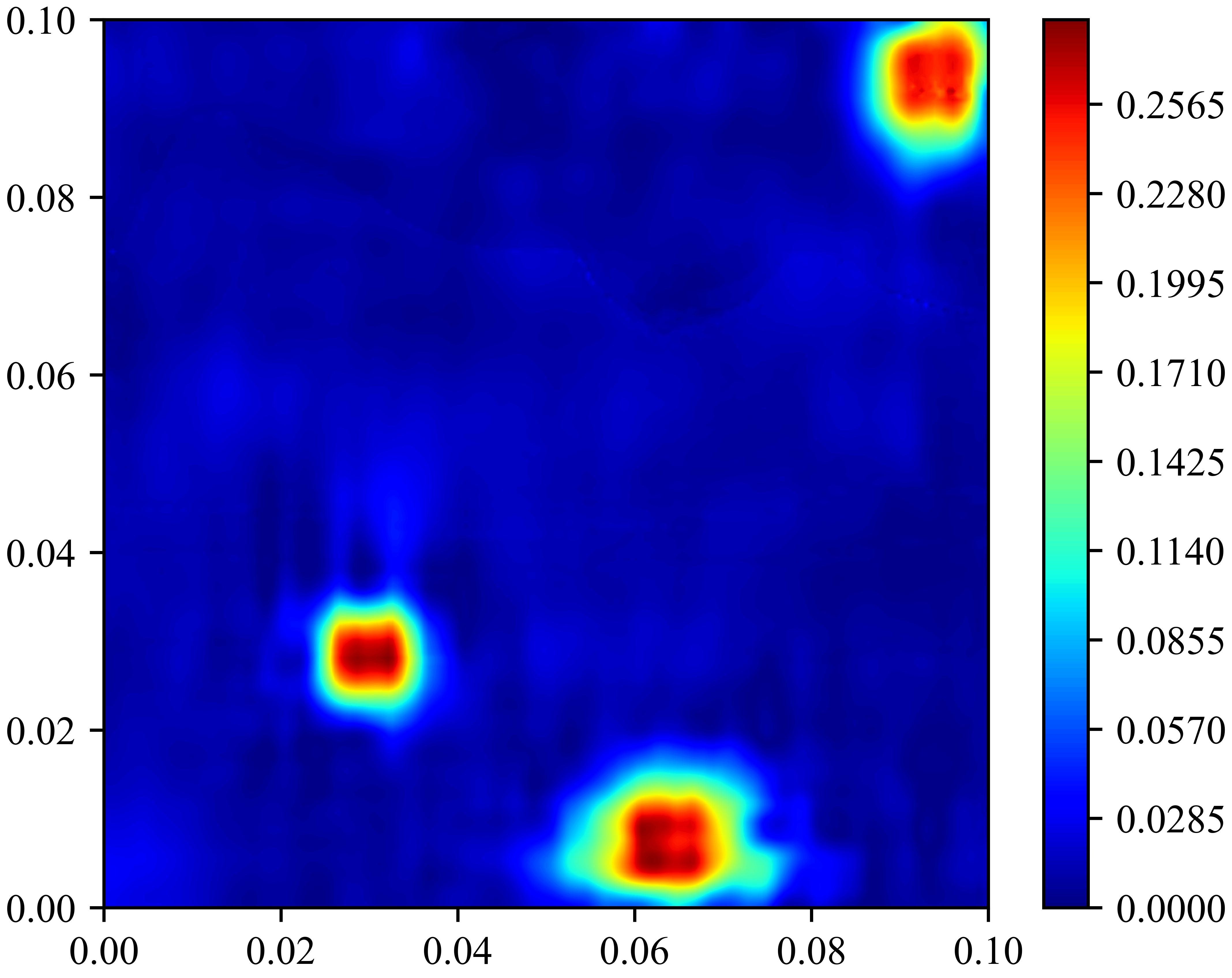
(d) Aleatoric uncertainty $\sigma_{4}^{{\varepsilon}_{1}}$

Figure 11: The quantified aleatoric uncertainties $\left\{\sigma_{1}^{{\varepsilon}_{1}},\sigma_{2}^{{\varepsilon}_{1}},\sigma_{3}^{{\varepsilon}_{1}},\sigma_{4}^{{\varepsilon}_{1}}\right\}$ for four MP temperatures $\left\{\bm{T}^{1*}_{MP},\bm{T}^{2*}_{MP},\bm{T}^{3*}_{MP},\bm{T}^{4*}_{MP}\right\}$ with the noise ${\varepsilon}_{1}\sim N\left(0,{0.25}^{2}\right)$ based on the model $\mathcal{M}^{{\varepsilon}_{1}}\left(\bm{T}_{MP},\bm{\tau};\bm{\theta}\right)$.

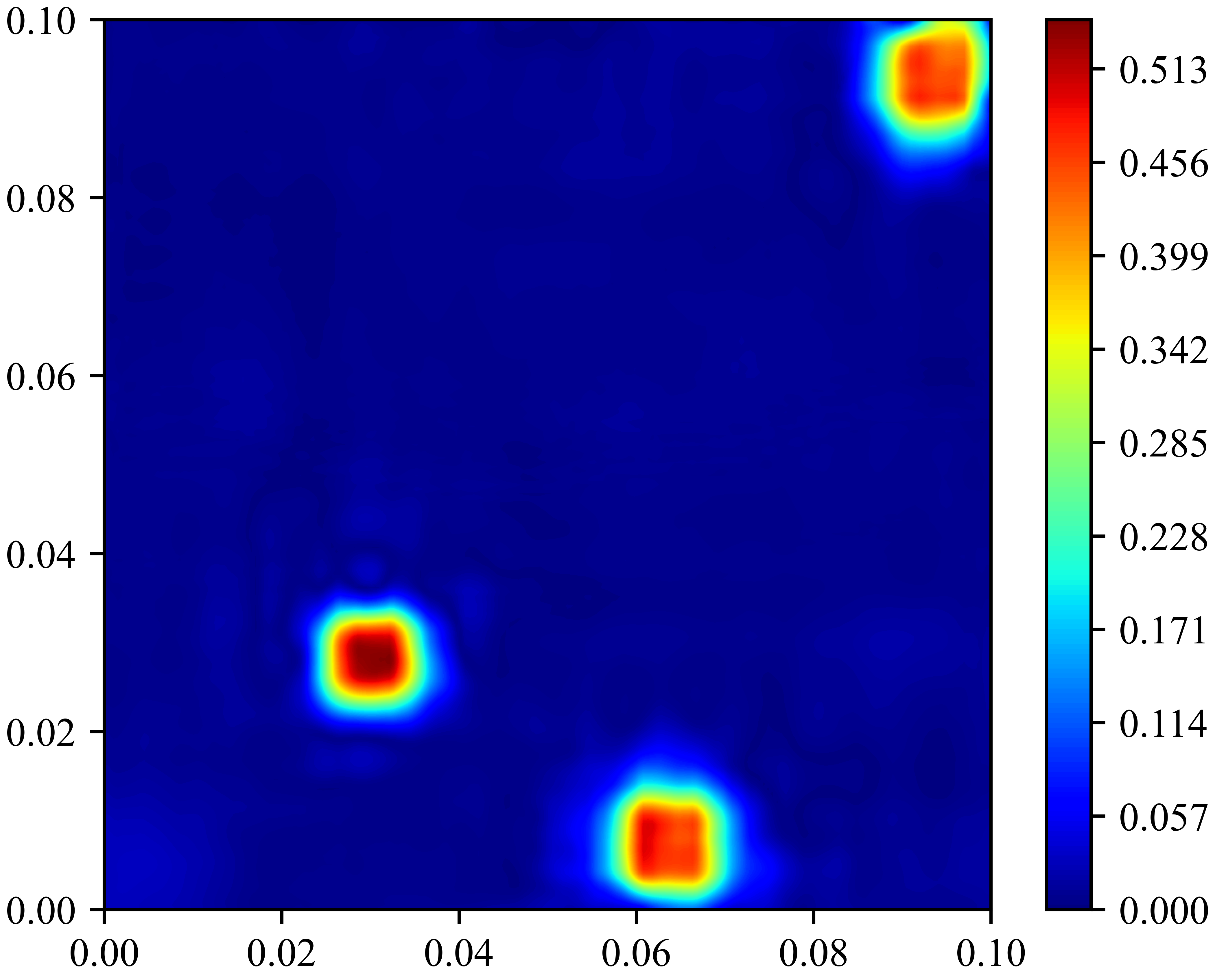
(a) Aleatoric uncertainty $\sigma_{1}^{{\varepsilon}_{2}}$

(b) Aleatoric uncertainty $\sigma_{2}^{{\varepsilon}_{2}}$

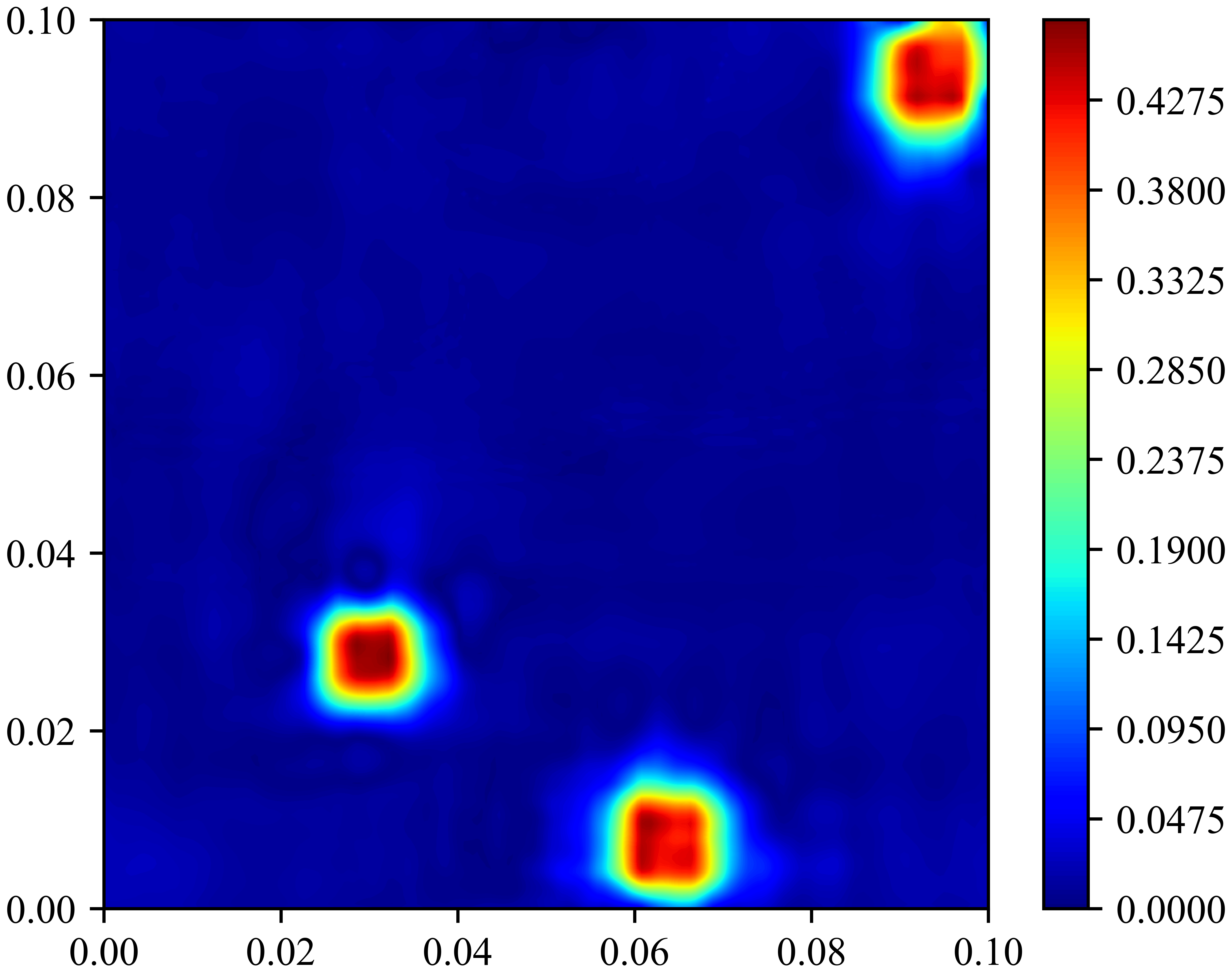
(c) Aleatoric uncertainty $\sigma_{3}^{{\varepsilon}_{2}}$

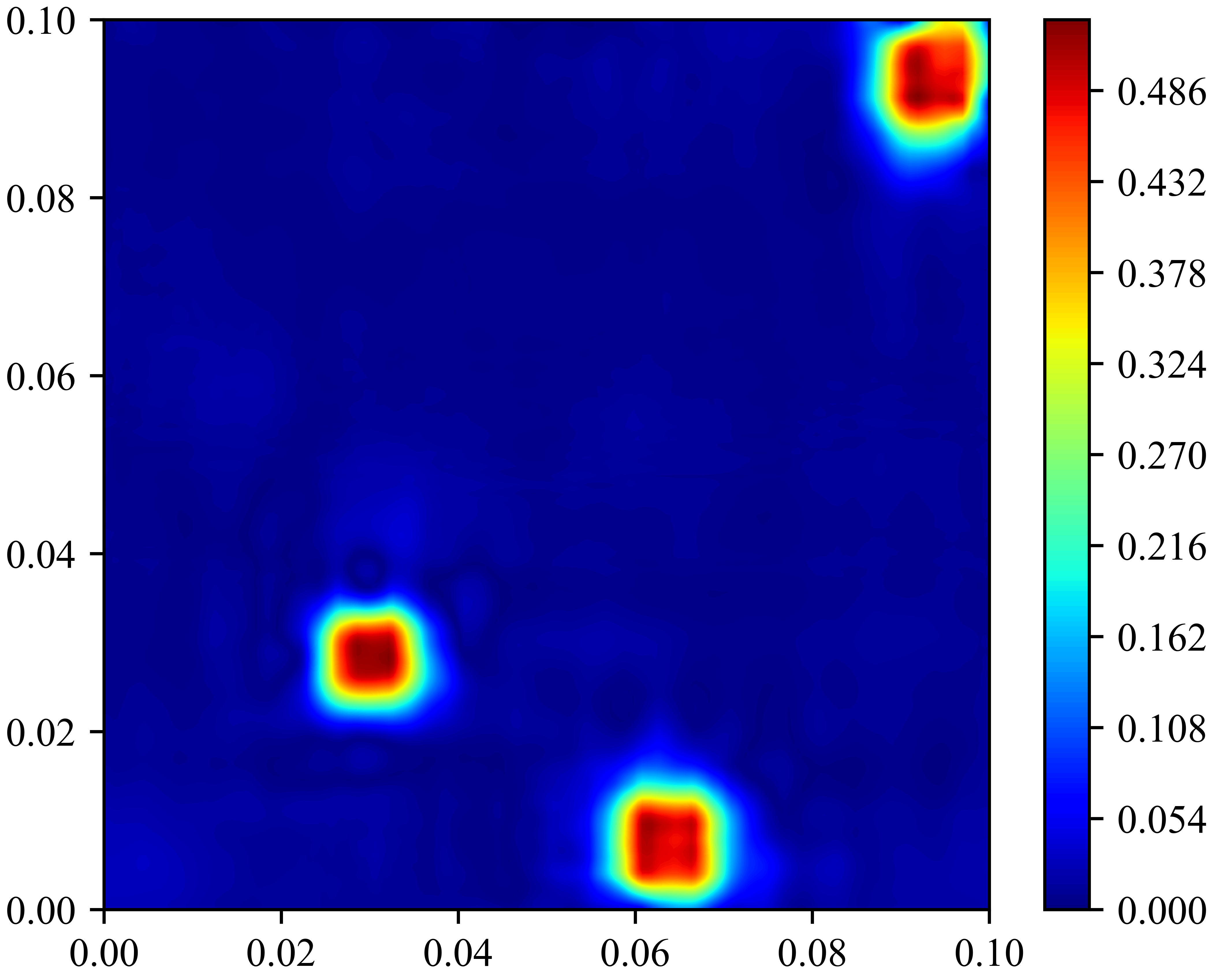
(d) Aleatoric uncertainty $\sigma_{4}^{{\varepsilon}_{2}}$

Figure 12: The quantified aleatoric uncertainties $\left\{\sigma_{1}^{{\varepsilon}_{2}},\sigma_{2}^{{\varepsilon}_{2}},\sigma_{3}^{{\varepsilon}_{2}},\sigma_{4}^{{\varepsilon}_{2}}\right\}$ for four MP temperatures $\left\{\bm{T}^{1*}_{MP},\bm{T}^{2*}_{MP},\bm{T}^{3*}_{MP},\bm{T}^{4*}_{MP}\right\}$ with the noise ${\varepsilon}_{1}\sim N\left(0,{0.5}^{2}\right)$ based on the model $\mathcal{M}^{{\varepsilon}_{2}}\left(\bm{T}_{MP},\bm{\tau};\bm{\theta}\right)$.

Necessity analysis of aleatoric uncertainty quantification

For four MP temperatures (Fig.9) whose monitoring points below the blue line in Fig.8 include the Gaussian noise ${\varepsilon}_{1}\sim N\left(0,{0.25}^{2}\right)$, the corresponding aleatoric uncertainties are quantified based on the model $\mathcal{M}^{b{\varepsilon}_{1}}\left(\bm{T}_{MP},\bm{\tau};\bm{\theta}\right)$ as shown in Figs.13. According to section 5.1.1, the model $\mathcal{M}^{b{\varepsilon}_{1}}\left(\bm{T}_{MP},\bm{\tau};\bm{\theta}\right)$ is trained by the dataset that includes the Gaussian noise ${\varepsilon}_{1}\sim N\left(0,{0.25}^{2}\right)$ in the monitoring points below the blue line in Fig.8.

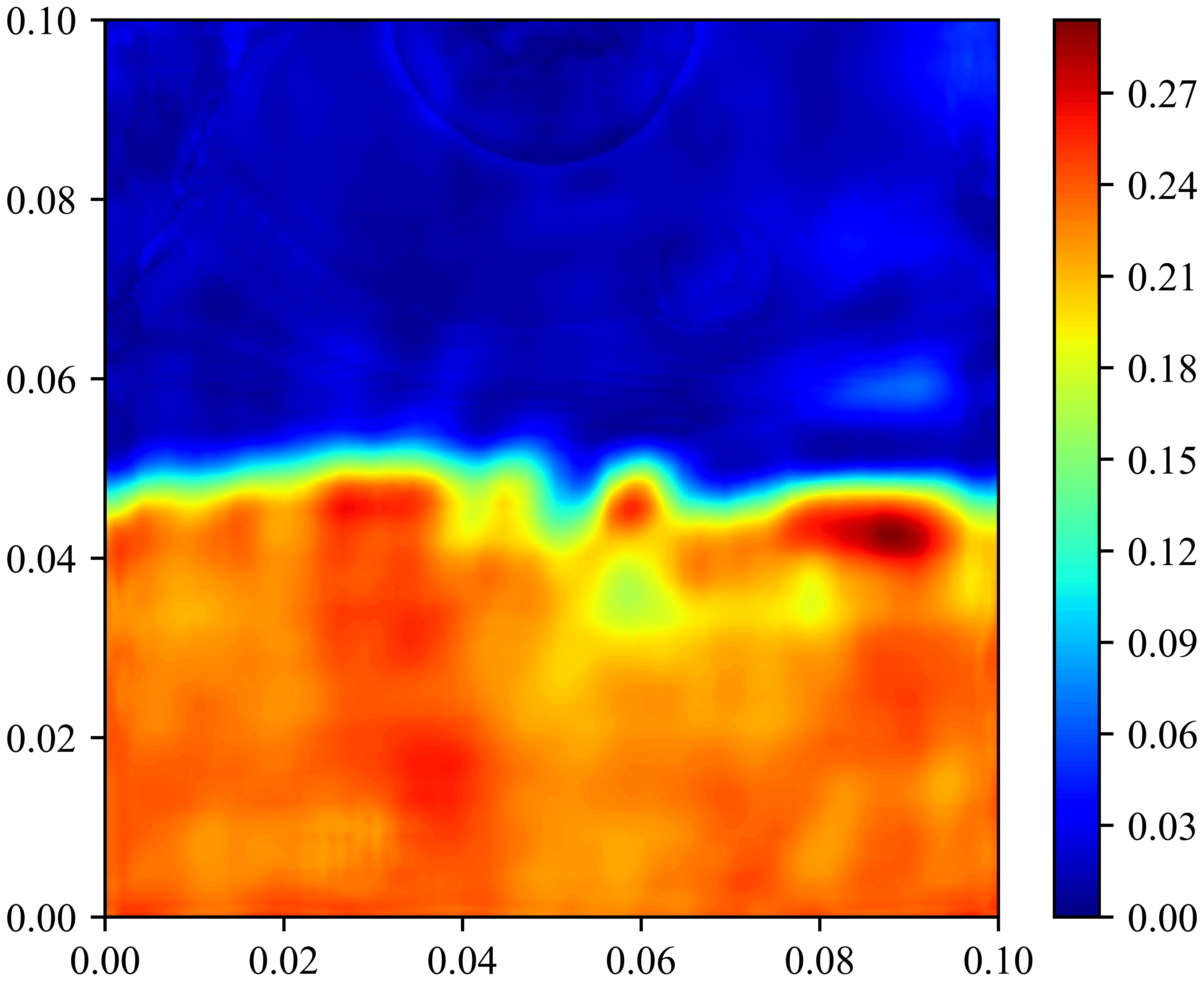
(a) Aleatoric uncertainty $\sigma_{1}^{b{\varepsilon}_{1}}$

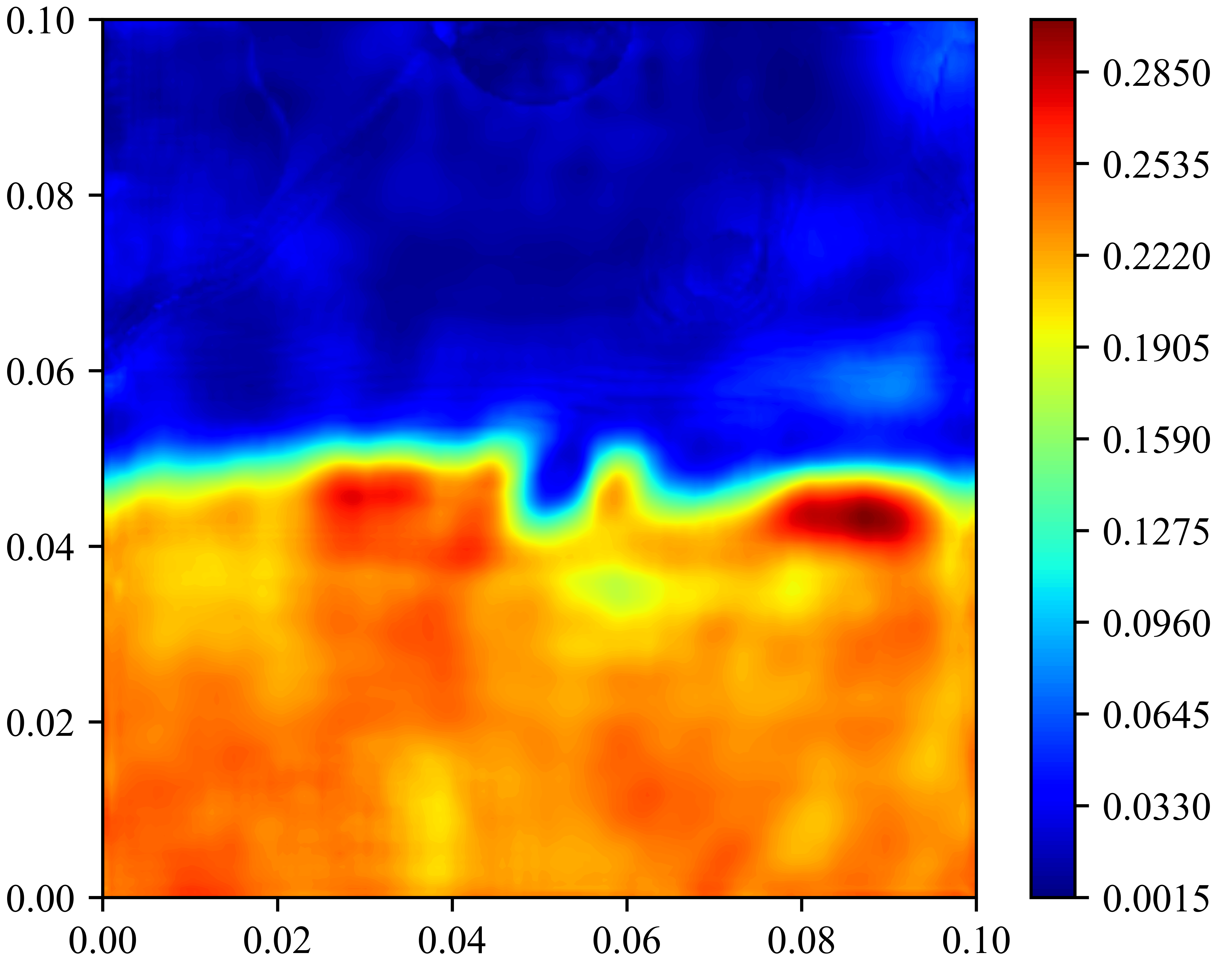
(b) Aleatoric uncertainty $\sigma_{2}^{b{\varepsilon}_{1}}$

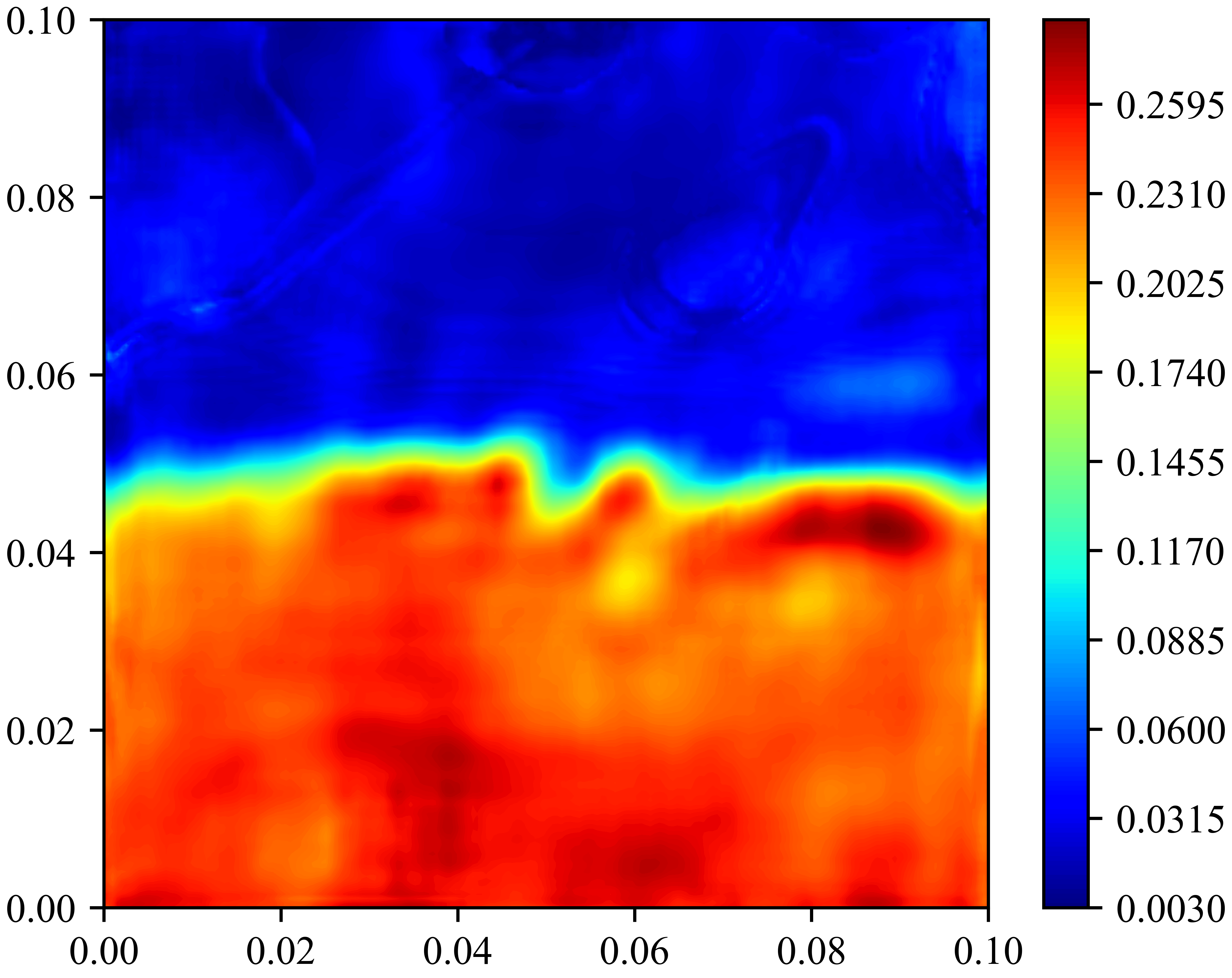
(c) Aleatoric uncertainty $\sigma_{3}^{b{\varepsilon}_{1}}$

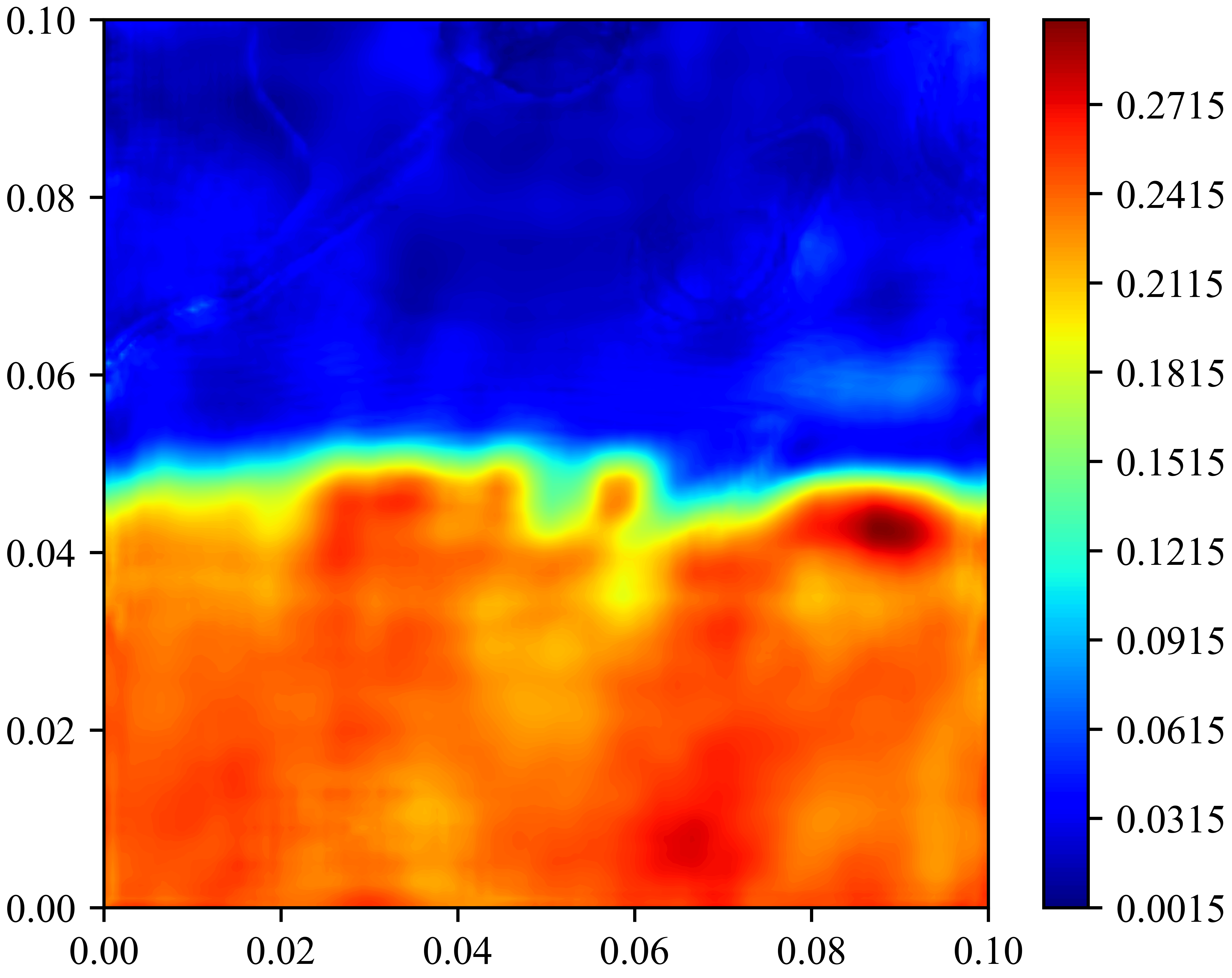
(d) Aleatoric uncertainty $\sigma_{4}^{b{\varepsilon}_{1}}$

Figure 13: The quantified aleatoric uncertainties $\left\{\sigma_{1}^{b{\varepsilon}_{1}},\sigma_{2}^{b{\varepsilon}_{1}},\sigma_{3}^{b{\varepsilon}_{1}},\sigma_{4}^{b{\varepsilon}_{1}}\right\}$ for four MP temperatures $\left\{\bm{T}^{1*}_{MP},\bm{T}^{2*}_{MP},\bm{T}^{3*}_{MP},\bm{T}^{4*}_{MP}\right\}$ with the noise ${\varepsilon}_{1}\sim N\left(0,{0.25}^{2}\right)$ based on the model $\mathcal{M}^{b{\varepsilon}_{1}}\left(\bm{T}_{MP},\bm{\tau};\bm{\theta}\right)$.

Refer to Fig.13, the aleatoric uncertainties corresponding to the area below the blue line are much larger than the area above the blue line. There are three pseudo-abnormal phenomenons in Fig.13 as follows:

(1) The maximum aleatoric uncertainty is abnormal. As shown in Fig.13, the max value of quantified aleatoric uncertainty is approximately equal to 0.3. However, the value of actual Gaussian noise is equal to 0.25.

(2) The aleatoric uncertainties of the non-monitoring point area below the blue line are abnormal. It is noteworthy that the aleatoric uncertainties of the non-monitoring point area below the blue line are also relatively large, as shown in Fig.14. However, the non-monitoring point area below the blue line does not contain Gaussian noise.

(3) It is abnormal for the magnitude of aleatoric uncertainty in some non-monitoring point areas to have large differences. As shown in Fig.14, the aleatoric uncertainty in the green dashed circle is larger than in the red dashed circle for the non-monitoring point area. However, there is no Gaussian noise in these two areas.

In fact, the above three pseudo-abnormal phenomenons are caused by the spread of data noise deviation. For the first pseudo-abnormal phenomenon, the spread of data noise leads to the accumulation of aleatoric uncertainty. Thereby, the maximum aleatoric uncertainty is larger than the actual Gaussian noise. For the second pseudo-abnormal phenomenon, the spread of data noise will transfer the aleatoric uncertainty to the surrounding area. Thus, the non-monitoring point area below the blue line contains aleatoric uncertainty. When the sensor measures temperature, the measured value is sometimes relatively large (positive Gaussian noise), and sometimes the measured value is relatively small (negative Gaussian noise). Thus for the third pseudo-abnormal phenomenon, the accumulation of positive or negative Gaussian noise will lead to the magnitude of aleatoric uncertainty in some non-monitoring point areas to large differences. For one thing, suppose the Gaussian noise of the measuring point in the area around the non-monitoring point is only positive or negative. In that case, the aleatoric uncertainty of the non-monitoring point area will be relatively large. For the other thing, suppose the Gaussian noise of the measuring point in the area around the non-monitoring point contains both positive and negative. In that case, the aleatoric uncertainty of the non-monitoring point area will be relatively small due to partial noise cancellation.

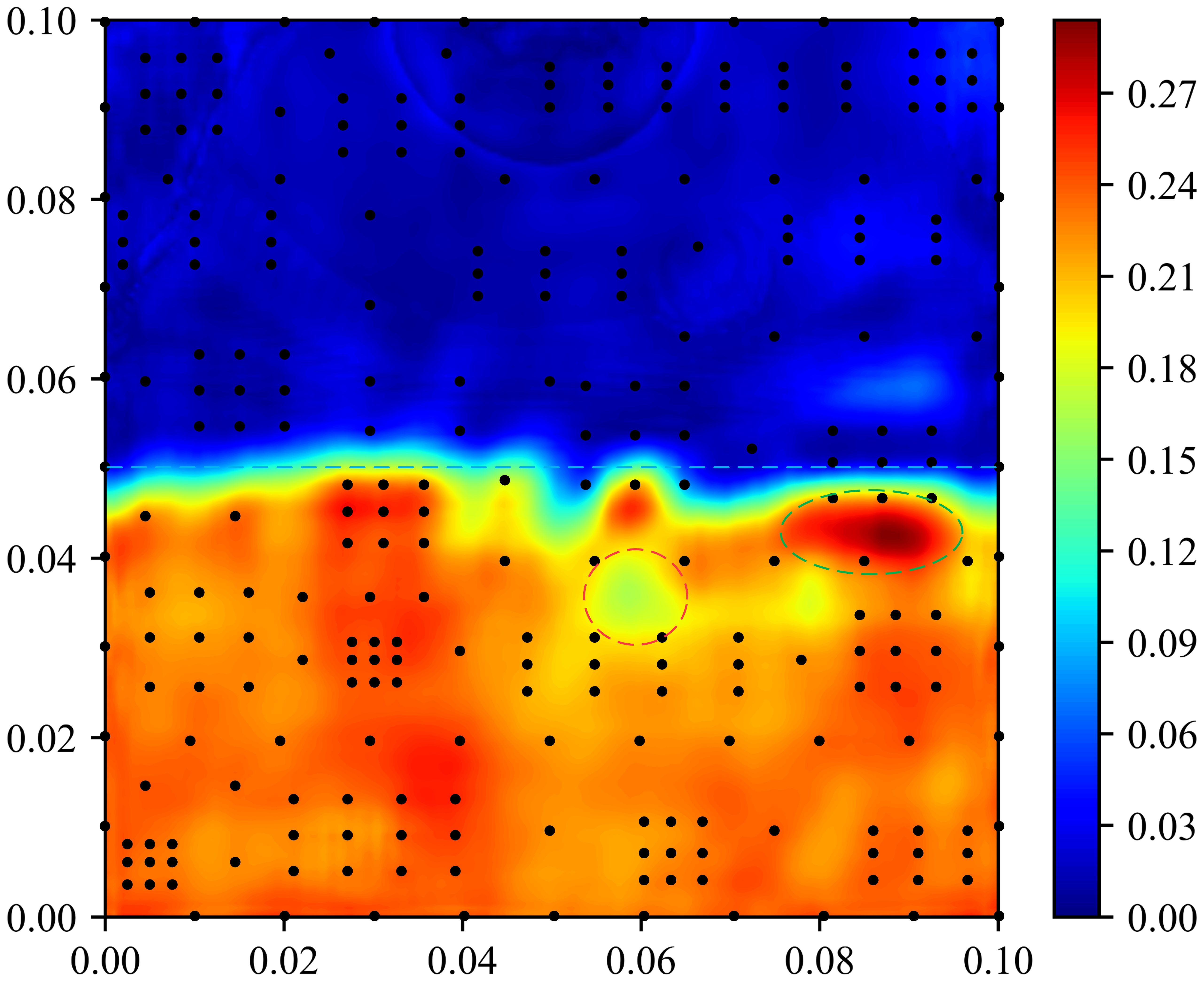
Figure 14: The fusion figure between the monitoring point position (Fig.8) and the quantified aleatoric uncertainty $\sigma_{1}^{b{\varepsilon}_{1}}$ (Fig. 13(a)).

In summary, the data noise of the monitoring point not only causes aleatoric uncertainty in its temperature prediction value but also leads to aleatoric uncertainty in the temperature prediction value of the surrounding area. Therefore, aleatoric uncertainty quantification is essential to ensure the credibility of the reconstructed temperature field for the satellite TFR problem.

5.2 Case 2: A satellite subsystem heat reliability analysis

5.2.1 Case background

The second case analyzes the heat reliability of a satellite subsystem. As shown in Fig.15, Fig.15 (a) is the satellite subsystem circuit board for installing 57 components, and Fig.15 (b) is the satellite component layout. The length $L$ is equal to 0.8m and the width $\delta$ of the heat sink is 0.112m. A total of 313 temperature monitoring points are arranged in this satellite subsystem, where the positions of all temperature monitoring points are shown in Fig.4 (c). As shown in Fig.16, the satellite subsystem $S$ includes 20 blocks, and each block is composed of some satellite components in a certain logical relationship. For example, the block $\mathcal{B}_{1}^{1}$ consists of components $\left\{C_{1},C_{2},C_{3}\right\}$ by the parallel relationship, the block $\mathcal{B}_{5}^{1}$ is composed of components $\left\{C_{16},C_{19}\right\}$ by the series relationships. Especially, the blocks $\mathcal{B}_{1}^{2}$, $\mathcal{B}_{2}^{2}$, and $\mathcal{B}_{3}^{2}$ are composed of blocks $\left\{\mathcal{B}_{1}^{1},\mathcal{B}_{2}^{1},\mathcal{B}_{3}^{1},\mathcal{B}_{4}^{1},\mathcal{B}_{5}^{1},\mathcal{B}_{17}^{1}\right\}$, $\left\{\mathcal{B}_{6}^{1},\mathcal{B}_{7}^{1},\mathcal{B}_{8}^{1},\mathcal{B}_{9}^{1},\mathcal{B}_{10}^{1}\right\}$, and $\left\{\mathcal{B}_{11}^{1},\mathcal{B}_{12}^{1},\mathcal{B}_{13}^{1},\mathcal{B}_{14}^{1},\mathcal{B}_{15}^{1},\mathcal{B}_{16}^{1}\right\}$ in the series relationship, respectively. The satellite subsystem $S$ consists of three blocks $\mathcal{B}_{1}^{2}$, $\mathcal{B}_{2}^{2}$, and $\mathcal{B}_{3}^{2}$ by the parallel relationship. The probability distributions of satellite component powers are shown in Table 4. Besides, the working state thresholds of 57 satellite components are also presented in Table 4.

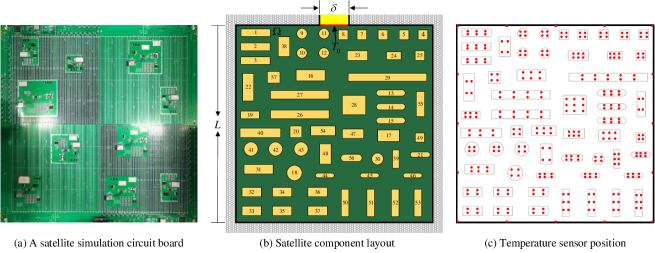
Figure 15: A satellite subsystem with 57 components in case 2.

Table 4: All satellite component powers’ probability distributions and working state thresholds in case 2.

S.C.	Mean	S.D.	Distribution	Threshold	S.C.	Mean	S.D.	Distribution	Threshold
$C_{1}$	195	8.3	Normal	322.60	$C_{31}$	180	6.5	Normal	330.10
$C_{2}$	195	8.3	Normal	322.90	$C_{32}$	197	13.8	Normal	330.80
$C_{3}$	195	8.3	Normal	323.60	$C_{33}$	197	13.8	Normal	333.10
$C_{4}$	136	5.7	Normal	321.05	$C_{34}$	197	13.8	Normal	330.70
$C_{5}$	136	5.7	Normal	320.30	$C_{35}$	197	13.8	Normal	331.00
$C_{6}$	136	5.7	Normal	318.10	$C_{36}$	197	13.8	Normal	330.30
$C_{7}$	136	5.7	Normal	313.82	$C_{37}$	197	13.8	Normal	330.60
$C_{8}$	136	5.7	Normal	308.65	$C_{38}$	164	5.8	Normal	321.00
$C_{13}$	186	8.8	Lognormal	324.30	$C_{39}$	167	5.1	Gumbel	328.60
$C_{14}$	186	8.8	Lognormal	325.40	$C_{41}$	138	2.9	Normal	329.20
$C_{15}$	186	8.8	Lognormal	326.40	$C_{42}$	138	2.9	Normal	329.00
$C_{16}$	172	7.8	Gumbel	322.30	$C_{43}$	138	2.9	Normal	328.90
$C_{17}$	172	7.8	Gumbel	327.50	$C_{47}$	194	6.4	Normal	327.30
$C_{18}$	167	6.3	Normal	330.00	$C_{48}$	87	5.7	Normal	329.00
$C_{20}$	139	5.4	Lognormal	328.00	$C_{49}$	134	2.8	Normal	327.50
$C_{21}$	135	4.1	Normal	328.30	$C_{50}$	193	17.1	Lognormal	330.20
$C_{22}$	96	5.2	Gumbel	325.80	$C_{51}$	193	17.1	Lognormal	330.00
$C_{23}$	168	4.9	Lognormal	317.90	$C_{52}$	193	17.1	Lognormal	329.90
$C_{25}$	141	3.9	Normal	321.90	$C_{53}$	193	17.1	Lognormal	329.70
$C_{26}$	218	6.6	Normal	326.80	$C_{54}$	159	3.5	Normal	327.40
$C_{27}$	218	6.6	Normal	325.30	$C_{55}$	147	4.2	Normal	326.00
$C_{28}$	202	8.9	Normal	325.50	$C_{57}$	137	6.4	Gumbel	324.00
$C_{29}$	313	9.7	Gumbel	323.50
S.C.	L.B.	U.B.	Distribution	Threshold	S.C.	L.B.	U.B.	Distribution	Threshold
$C_{9}$	82	121	Uniform	316.10	$C_{30}$	60	133	Uniform	328.60
$C_{10}$	82	121	Uniform	318.30	$C_{40}$	110	180	Uniform	328.40
$C_{11}$	82	121	Uniform	309.03	$C_{44}$	78	143	Uniform	329.60
$C_{12}$	82	121	Uniform	315.50	$C_{45}$	78	143	Uniform	329.20
$C_{19}$	67	139	Uniform	327.00	$C_{46}$	78	143	Uniform	329.00
$C_{24}$	90	147	Uniform	321.00	$C_{56}$	121	160	Uniform	328.70
S.C. = Satellite component   S.D. = Standard deviation   L.B. = Lower boundary
U.B. = Upper boundary

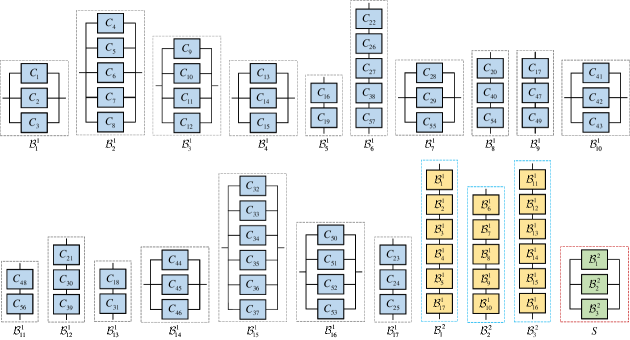
Figure 16: The logical relationships between satellite components ($C$), blocks ($\mathcal{B}$), and satellite subsystem ($S$).

5.2.2 Deep MC-QR model training and results analysis

Preparing data and training model

According to the component powers’ probability distributions, this case samples 10000 sets of component powers by the Latin Hypercube Sampling, and based on this, 10000 satellite subsystem operating conditions are set. Then, 10000 ground simulation experiments are carried out based on a satellite simulation system. For each simulation experiment, these temperature values of all points in Fig.4 (c) are measured by 313 sensors when the satellite simulation system arrives at steady-state. Finally, the ground simulation experiment can obtain 10000 MP temperatures $\left\{\bm{T}^{1}_{MP},\bm{T}^{2}_{MP},\cdots,\bm{T}^{10000}_{MP}\right\}$. The sensor measurement deviation is about $\pm 0.15\text{K}$. In this case, 8100 MP temperatures are used to train the physics-informed Deep MC-QR model $\mathcal{M}\left(\bm{T}_{MP},\bm{\tau};\bm{\theta}\right)$, 900 MP temperatures are used to be the validate data, and the remaining 1000 MP temperatures are used to test the trained model $\mathcal{M}\left(\bm{T}_{MP},\bm{\tau};\bm{\theta}\right)$. For the 1000 testing MP temperatures, the corresponding approximate truth temperature fields can be obtained by the infrared camera. In this case, the maximum training epoch and the learning rate are set to be 80 and 0.1, respectively. Based on the prepared training dataset, the trained model $\mathcal{M}\left(\bm{T}_{MP}\right)$ is obtained by the Algorithm 1.

Predicted results analysis

According to four indicators in section 3.4, three kinds of average errors $\overline{RMSE}$, $\overline{MAE}$ and $\overline{MRE}$ are 0.0524, 0.0414, and 0.0001, respectively. Besides, the $\overline{R^{2}}$ value of the trained model is 0.9999. For the MP temperature in Fig.17(a), its truth temperature field, reconstructed temperature field, and aleatoric uncertainty are shown in Fig.17(b), Fig.17(c), and Fig.17(d), respectively. Comparing Fig.17(b) and Fig.17(c), the reconstructed temperature field is basically consistent with the truth temperature field. For Fig.17(d), the maximum value of quantified aleatoric uncertainty is approximately equal to 0.17. Thereby, the maximum difference between the quantified aleatoric uncertainty and the sensor measurement absolute deviation (0.15) is about 0.02. According to the necessity analysis of aleatoric uncertainty quantification in section 5.1.2, the difference of 0.02 is mainly caused by the spread of data noise deviation. Besides, it is noteworthy that the quantified aleatoric uncertainties in the top heat sink area ($\Omega_{BC}$) and its surrounding non-monitoring point areas are almost equal to 0. Because the loss function (Eq.(24)) of the training model uses boundary condition (Eq.(10)), the temperature value of area $\Omega_{BC}$ is not affected by data noise. Therefore, the aleatoric uncertainties in area $\Omega_{BC}$ and its surrounding non-monitoring point areas are very small.

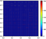
(a) MP temperature

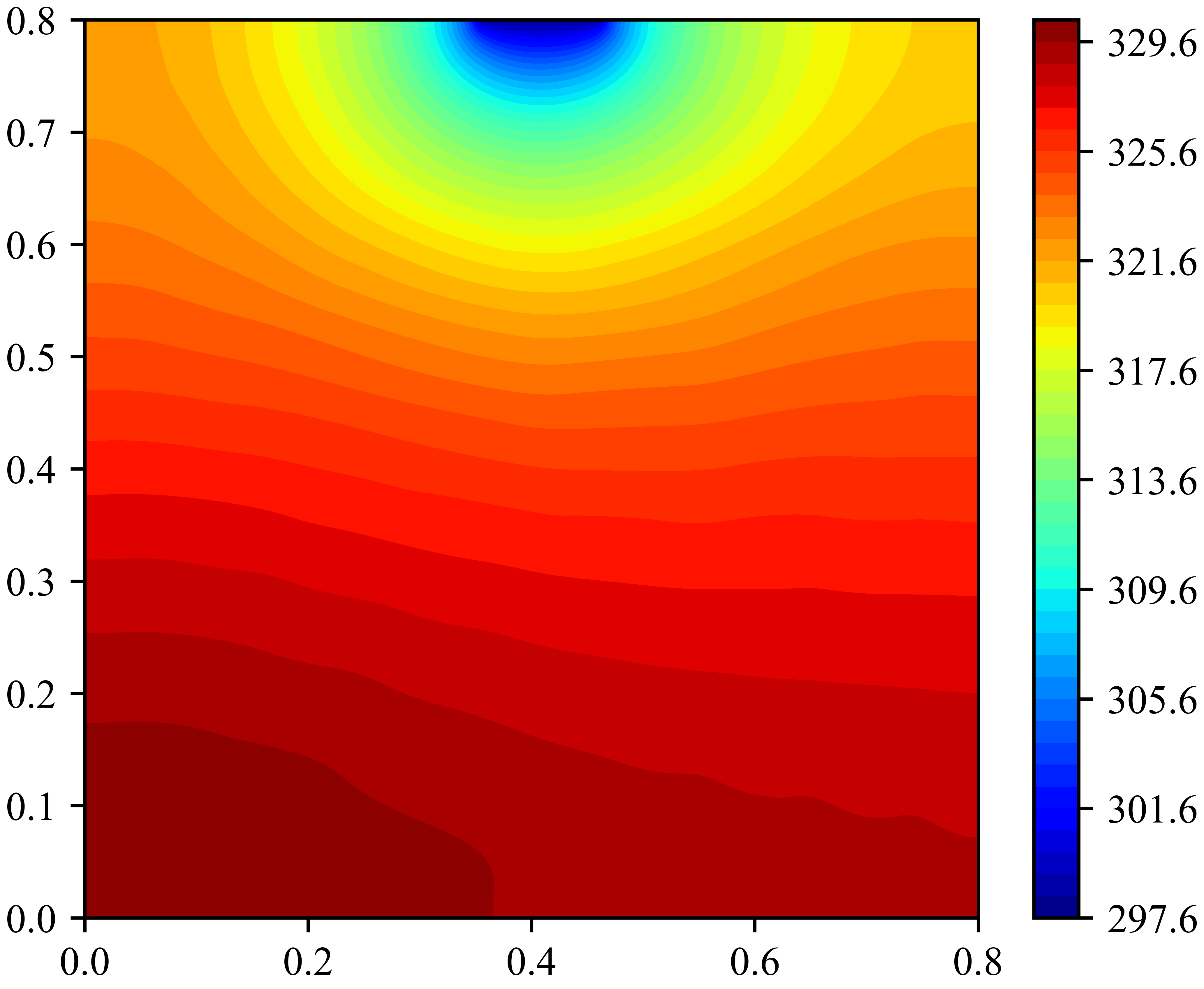
(b) Truth temperature field

(c) Reconstructed temperature field

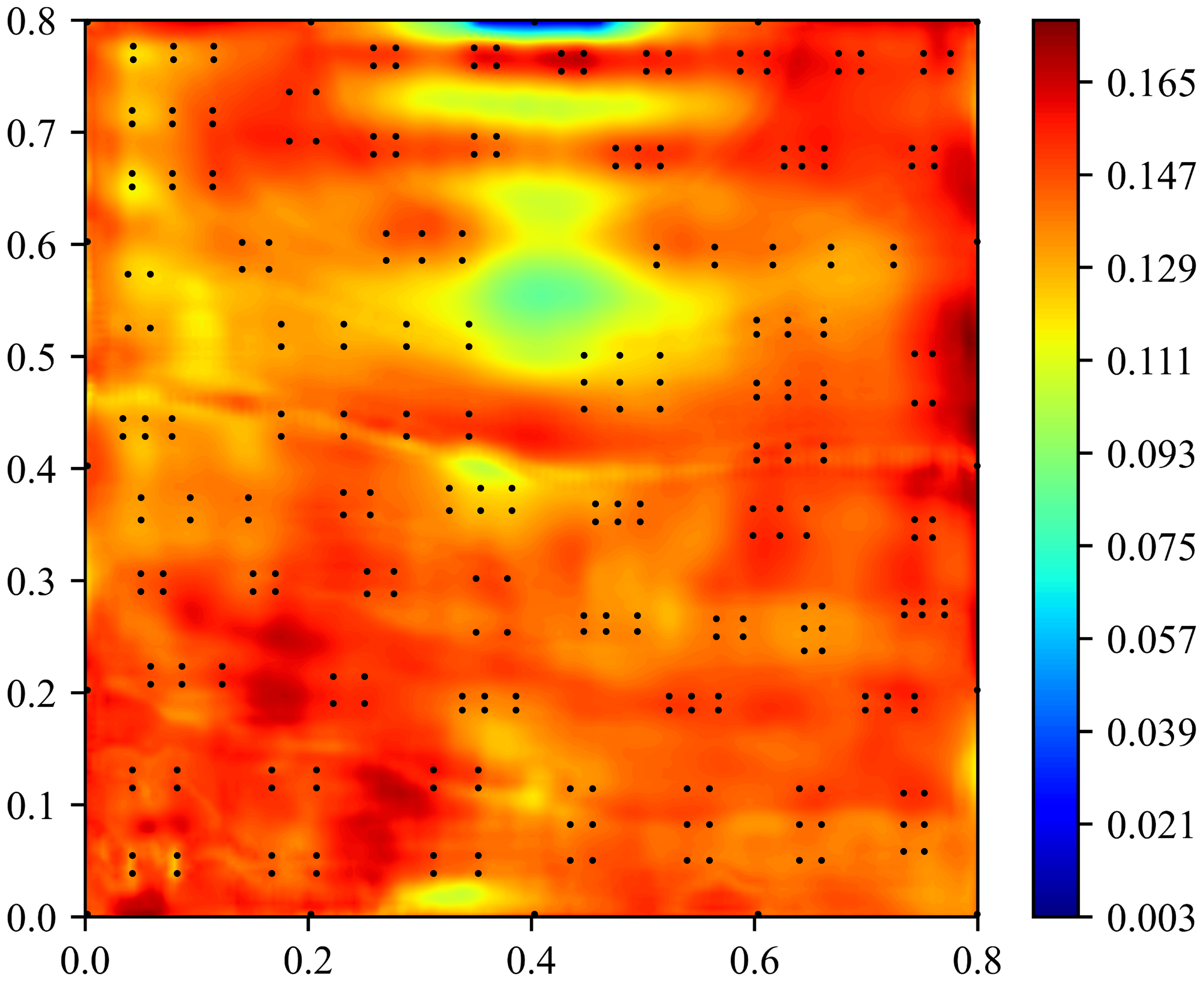
(d) Aleatoric uncertainty

Figure 17: A MP temperature and its truth temperature field, reconstructed temperature field, and aleatoric uncertainty. The black points in (d) are the temperature monitoring points.

In summary, the proposed physics-informed Deep MC-QR method can construct an accurate surrogate model to reconstruct the temperature field of the satellite subsystem and can quantify the aleatoric uncertainty precisely. Thus, the reconstructed temperature field and the quantified aleatoric uncertainty are used to analyze the heat reliability of the satellite subsystem (Fig.15) based on the interval multilevel BN in the following sections.

5.2.3 Interval 4-level BN modeling

For this case, the hyperparameter $\lambda$ is set to be 1.0, i.e., $\lambda=1.0$, and $1\times 10^{5}$ discretized MP temperature images are used to estimate the probability distributions of satellite components, i.e., $N_{MCS}=1\times 10^{5}$. Based on $1\times 10^{5}$ reconstructed temperature fields, the cumulative distribution function of each satellite component can be estimated. For example, the cumulative distribution functions of satellite components $C_{1}$, $C_{10}$, $C_{20}$, $C_{30}$, $C_{40}$, and $C_{57}$ are shown in Fig.18. By Algorithm 3, the satellite components’ normal probability intervals are estimated as shown in Table 5. If the aleatoric uncertainty of the reconstructed temperature field is ignored, i.e., $\lambda=0$, the satellite components’ normal probabilities $\left\{Pr_{\lambda=0}^{C_{s}=1}|s=1,2,\cdots,57\right\}$ are calculated based on the reconstructed temperature fields $\left\{{\hat{\bm{T}}}_{pre}^{m}|m=1,2,\cdots,10^{5}\right\}$ and the working state thresholds, as shown in Table 5.

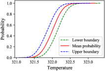
(a) Satellite component $C_{1}$

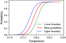
(b) Satellite component $C_{10}$

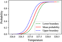
(c) Satellite component $C_{20}$

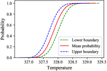
(d) Satellite component $C_{30}$

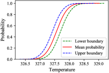
(e) Satellite component $C_{40}$

(f) Satellite component $C_{57}$

Figure 18: The cumulative distribution functions of satellite components $C_{1}$, $C_{10}$, $C_{20}$, $C_{30}$, $C_{40}$, and $C_{57}$.

Table 5: The estimated satellite components’ (interval) normal probabilities in case 2.

S.C.	$Pr_{\lambda=0}^{C_{s}=1}$	N.P. interval	S.C.	$Pr_{\lambda=0}^{C_{s}=1}$	N.P. interval	S.C.	$Pr_{\lambda=0}^{C_{s}=1}$	N.P. interval
$C_{1}$	0.9944	$\left[0.9746,0.9991\right]$	$C_{20}$	0.9987	$\left[0.9926,0.9998\right]$	$C_{39}$	0.9758	$\left[0.9246,0.9942\right]$
$C_{2}$	0.9888	$\left[0.9550,0.9981\right]$	$C_{21}$	0.9967	$\left[0.9850,0.9995\right]$	$C_{40}$	0.9976	$\left[0.9893,0.9997\right]$
$C_{3}$	0.9987	$\left[0.9913,0.9998\right]$	$C_{22}$	0.9984	$\left[0.9890,0.9997\right]$	$C_{41}$	0.9846	$\left[0.9507,0.9965\right]$
$C_{4}$	0.9973	$\left[0.9819,0.9996\right]$	$C_{23}$	0.9973	$\left[0.9778,0.9997\right]$	$C_{42}$	0.9778	$\left[0.9363,0.9945\right]$
$C_{5}$	0.9966	$\left[0.9764,0.9996\right]$	$C_{24}$	0.9980	$\left[0.9857,0.9998\right]$	$C_{43}$	0.9959	$\left[0.9836,0.9994\right]$
$C_{6}$	0.9907	$\left[0.9437,0.9990\right]$	$C_{25}$	0.9879	$\left[0.9437,0.9981\right]$	$C_{44}$	0.9950	$\left[0.9800,0.9992\right]$
$C_{7}$	0.9924	$\left[0.9399,0.9994\right]$	$C_{26}$	0.9916	$\left[0.9685,0.9986\right]$	$C_{45}$	0.9948	$\left[0.9800,0.9991\right]$
$C_{8}$	0.9985	$\left[0.9666,0.9999\right]$	$C_{27}$	0.9975	$\left[0.9850,0.9998\right]$	$C_{46}$	0.9903	$\left[0.9681,0.9979\right]$
$C_{9}$	0.9959	$\left[0.9599,0.9998\right]$	$C_{28}$	0.9980	$\left[0.9885,0.9997\right]$	$C_{47}$	0.9959	$\left[0.9820,0.9993\right]$
$C_{10}$	0.9870	$\left[0.9267,0.9987\right]$	$C_{29}$	0.9911	$\left[0.9644,0.9983\right]$	$C_{48}$	0.9957	$\left[0.9824,0.9993\right]$
$C_{11}$	0.9967	$\left[0.9410,0.9999\right]$	$C_{30}$	0.9957	$\left[0.9818,0.9993\right]$	$C_{49}$	0.9940	$\left[0.9780,0.9987\right]$
$C_{12}$	0.9960	$\left[0.9657,0.9997\right]$	$C_{31}$	0.9930	$\left[0.9759,0.9986\right]$	$C_{50}$	0.9903	$\left[0.9676,0.9978\right]$
$C_{13}$	0.9868	$\left[0.9516,0.9977\right]$	$C_{32}$	0.9915	$\left[0.9699,0.9980\right]$	$C_{51}$	0.9906	$\left[0.9671,0.9982\right]$
$C_{14}$	0.9912	$\left[0.9616,0.9986\right]$	$C_{33}$	0.9952	$\left[0.9833,0.9991\right]$	$C_{52}$	0.9884	$\left[0.9642,0.9972\right]$
$C_{15}$	0.9917	$\left[0.9684,0.9981\right]$	$C_{34}$	0.9968	$\left[0.9865,0.9994\right]$	$C_{53}$	0.9722	$\left[0.9273,0.9908\right]$
$C_{16}$	0.9906	$\left[0.9504,0.9990\right]$	$C_{35}$	0.9978	$\left[0.9904,0.9997\right]$	$C_{54}$	0.9881	$\left[0.9568,0.9979\right]$
$C_{17}$	0.9959	$\left[0.9827,0.9993\right]$	$C_{36}$	0.9915	$\left[0.9711,0.9981\right]$	$C_{55}$	0.9966	$\left[0.9858,0.9991\right]$
$C_{18}$	0.9944	$\left[0.9788,0.9990\right]$	$C_{37}$	0.9943	$\left[0.9768,0.9991\right]$	$C_{56}$	0.9975	$\left[0.9881,0.9996\right]$
$C_{19}$	0.9895	$\left[0.9625,0.9981\right]$	$C_{38}$	0.9951	$\left[0.9703,0.9995\right]$	$C_{57}$	0.9969	$\left[0.9816,0.9997\right]$

According to the logical relationships between satellite components, blocks, and satellite subsystem in Fig.16, this case model an interval 4-level BN for satellite system heat reliability analysis as shown in Fig.19. The interval probability distributions of the root nodes are shown in Table 5. For the child nodes, their CPTs can be obtained by the series or parallel relationships. For example, the CPT of a child node with parallel parent nodes is shown in Table 1. Thereby, the satellite subsystem reliability interval can be inferred based on the interval 4-level BN.

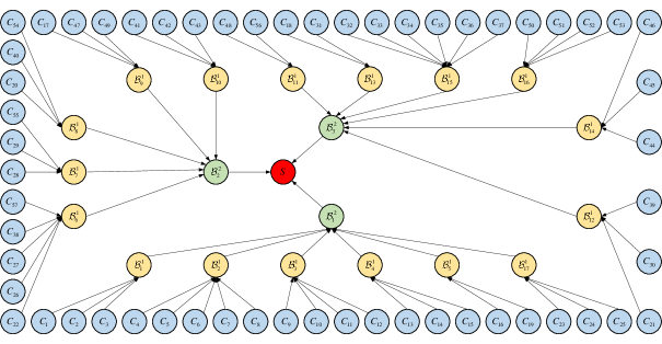
Figure 19: Interval 4-level BN for satellite system heat reliability analysis.

5.2.4 Heat reliability analysis

Inferred by the interval 4-level BN, the normal probability intervals of blocks $\mathcal{B}_{1}^{2}$, $\mathcal{B}_{2}^{2}$ and $\mathcal{B}_{3}^{2}$ are shown in Table 6, and the satellite subsystem interval heat reliability $\widetilde{R}$ is $\left[0.99416447,0.99999952\right]$, i.e., $\widetilde{R}=\left[0.99416447,0.99999952\right]$. If the aleatoric uncertainty of the reconstructed temperature field is ignored ($\lambda=0$), the satellite subsystem heat reliability $R_{\lambda=0}$ is 0.99991071, i.e., $R_{\lambda=0}=0.99991071$. Apparently, $R_{\lambda=0}\in\widetilde{R}$. Suppose that the engineers use the result $R_{\lambda=0}=0.99991071$ to evaluate the satellite subsystem heat reliability. This may lead to the following problems. If the temperature measured by the sensor is a relatively large truth temperature, the result $R_{\lambda=0}=0.99991071$ will be less than the truth heat reliability, i.e., underestimating the satellite subsystem heat reliability. Otherwise, the result $R_{\lambda=0}=0.99991071$ will be more than the truth heat reliability, i.e., overestimating the satellite subsystem heat reliability. However, the above problems will not occur when engineers use $\widetilde{R}=\left[0.99416447,0.99999952\right]$ to evaluate the satellite subsystem heat reliability. Besides, $\widetilde{R}=\left[0.99416447,0.99999952\right]$ contains the lowest and highest heat reliability of the satellite subsystem. Therefore, the interval heat reliability $\widetilde{R}$ can provide engineers with more reliable information to design this satellite subsystem.

Table 6: The normal probability intervals of blocks $\mathcal{B}_{1}^{2}$, $\mathcal{B}_{1}^{2}$ and $\mathcal{B}_{1}^{2}$ in case 2.

Block	$\mathcal{B}_{1}^{2}$	$\mathcal{B}_{2}^{2}$	$\mathcal{B}_{2}^{2}$
N.P. interval	$\left[0.8320,0.9947\right]$	$\left[0.7968,0.9920\right]$	$\left[0.8291,0.9894\right]$

As shown in Table 7, this case studies the influence of the block $\mathcal{B}_{1}^{2}$ ( or $\mathcal{B}_{2}^{2}$, or $\mathcal{B}_{3}^{2}$) failure on satellite subsystem (interval) heat reliability $R^{E}_{\lambda=0}$ ($\widetilde{R}^{E}$). For $\lambda=0$, the heat reliability $R^{E}_{\lambda=0}$ under any piece of evidence in Table 7 is less than $R_{\lambda=0}=0.99991071$. Compared with $\widetilde{R}=\left[0.99416447,0.99999952\right]$, the failure of block $\mathcal{B}_{1}^{2}$ ( or $\mathcal{B}_{2}^{2}$, or $\mathcal{B}_{3}^{2}$) reduces the satellite subsystem interval heat reliability $\widetilde{R}^{E}$. For one thing, according to the interval number size comparison formula [54], the order of three interval numbers in Table 7 is $\left[0.96527106,0.99991542\right]<\left[0.96585417,0.99995774\right]<\left[0.97128373,0.99994403\right]$, which means that the failure of block $\mathcal{B}_{2}^{2}$ has the lowest impact on the satellite subsystem heat reliability. For another thing, judging from the values of $R^{E}_{\lambda=0}$, the satellite subsystem heat reliability is least affected by the failure of block $\mathcal{B}_{3}^{2}$. Apparently, the above two conclusions are contradictory. Detailed comparison shows that $R^{E\left(\mathcal{B}_{2}^{2}=0\right)}_{\lambda=0}=0.99818277$ is very close to $R^{E\left(\mathcal{B}_{3}^{2}=0\right)}_{\lambda=0}=0.99822152$. Due to the presence of data noise, the above second conclusion may not be robust. Thus, it is more believable to use interval numbers to analyze the influence of block failure on satellite subsystem heat reliability.

Table 7: The satellite subsystem (interval) heat reliability $R^{E}_{\lambda=0}$ ($\widetilde{R}^{E}$) under different evidences in case 2.

Evidence	$\mathcal{B}_{1}^{2}=0$	$\mathcal{B}_{2}^{2}=0$	$\mathcal{B}_{3}^{2}=0$
$R^{E}_{\lambda=0}$	0.99753356	0.99818277	0.99822152
$\widetilde{R}^{E}$	$\left[0.96527106,0.99991542\right]$	$\left[0.97128373,0.99994403\right]$	$\left[0.96585417,0.99995774\right]$

6 Conclusions

This paper proposes the physics-informed Deep MC-QR method for reconstructing temperature field and quantifying the aleatoric uncertainty. For one thing, the proposed method combines a deep convolutional neural network with the known physics knowledge to reconstruct an accurate temperature field using some unlabeled monitoring point temperatures. For another thing, the proposed method can quantify the aleatoric uncertainty by the Monte Carlo quantile regression. Based on the reconstructed temperature field and the quantified aleatoric uncertainty, the normal probability interval of each satellite component is obtained by implementing the Monte Carlo simulation on the trained physics-informed Deep MC-QR model. Thereby, this paper models an interval multilevel BN to analyze satellite heat reliability. Two case studies are used for verifying the effectiveness of the proposed methods. The results of the first case study show that the proposed physics-informed Deep MC-QR method can accurately reconstruct the temperature field and precisely quantify the aleatoric uncertainty caused by data noise. The second case study validates that interval heat reliability can provide engineers with more reliable information to design a satellite subsystem.

In summary, this paper has the following three innovations: (1) The proposed physics-informed Deep MC-QR method can reconstruct an accurate temperature field using only monitoring point temperatures combined with the known physics knowledge; (2) Based on the Monte Carlo quantile regression, the proposed physics-informed Deep MC-QR method can precisely quantify the aleatoric uncertainty caused by data noise; (3) The interval multilevel BN can infer the satellite heat reliability using the reconstructed temperature field and the quantified aleatoric uncertainty. Generally, the positions of monitoring points are very important for the TFR problem. Therefore, the authors will explore how to choose the monitoring points’ positions to improve further the accuracy of the reconstructed temperature field in future research.

Appendix A Parallel block’s normal probability interval

For the parallel block $\mathcal{B}_{pa}$ in Fig.6, the state combinations of all components $\left\{{{C}_{\stackrel{{\scriptstyle\frown}}{{s}}}}|{\stackrel{{\scriptstyle\frown}}{{s}}}=1,2,\cdots,\stackrel{{\scriptstyle\frown}}{{n}}\right\}$ are determined by the format in these references [3, 4]. Therefore, the CPT $\Pr\left(\mathcal{B}_{pa}|{C_{1}},{C_{2}},\cdots,{C_{\stackrel{{\scriptstyle\frown}}{{n}}}}\right)$ of parallel block $\mathcal{B}_{pa}$ is shown in Table 1.

Table 1: The CPT $\Pr\left(\mathcal{B}_{pa}|{C_{1}},{C_{2}},\cdots,{C_{\stackrel{{\scriptstyle\frown}}{{n}}}}\right)$ of the parallel block $\mathcal{B}_{pa}$.

$C_{1}$	$C_{2}$	$\cdots$	${C_{\stackrel{{\scriptstyle\frown}}{{n}}-1}}$	$C_{\stackrel{{\scriptstyle\frown}}{{n}}}$	$\Pr\left(\mathcal{B}_{pa}|{C_{1}},{C_{2}},\cdots,{C_{\stackrel{{\scriptstyle\frown}}{{n}}}}\right)$
					$\mathcal{B}_{pa}=0$	$\mathcal{B}_{pa}=1$
0	0	$\cdots$	0	0	1	0
0	0	$\cdots$	0	1	0	1
0	0	$\cdots$	1	0	0	1
0	0	$\cdots$	1	1	0	1
$\vdots$	$\vdots$	$\vdots$	$\vdots$	$\vdots$	$\vdots$	$\vdots$
1	1	$\cdots$	0	0	0	1
1	1	$\cdots$	0	1	0	1
1	1	$\cdots$	1	0	0	1
1	1	$\cdots$	1	1	0	1

Refer to Table 1, the normal conditional probability $\Pr\left(\mathcal{B}_{pa}=1|{C_{1}},{C_{2}},\cdots,{C_{\stackrel{{\scriptstyle\frown}}{{n}}}}\right)$ is denoted as

$$\Pr\left(\mathcal{B}_{pa}=1|{C_{1}},{C_{2}},\cdots,{C_{\stackrel{{\scriptstyle\frown}}{{n}}}}\right)=\left\{0,\underbrace{1,\cdots 1}_{{{2}^{\stackrel{{\scriptstyle\frown}}{{n}}}}-1}\right\}.$$ (49)

For the parallel block $\mathcal{B}_{pa}$ in Fig.6, the calculation formulas (${\stackrel{{\scriptstyle\frown}}{{n}}}=2$ and ${\stackrel{{\scriptstyle\frown}}{{n}}}\geq 3$) of the normal probability interval $\widetilde{\Pr}\left(\mathcal{B}_{pa}=1\right)$ are presented as follows.

If ${\stackrel{{\scriptstyle\frown}}{{n}}}=2$,

$$\widetilde{\Pr}\left({{\mathcal{B}}_{pa}}=1\right)=\widetilde{\Pr}\left({{C}_{1}}=0\right)\widetilde{\Pr}\left({{C}_{2}}=1\right)+\widetilde{\Pr}\left({{C}_{1}}=1\right)$$ (50)

$$\qquad\qquad\quad\;\,=\left[1-\widetilde{\Pr}\left({{C}_{1}}=1\right)\right]\widetilde{\Pr}\left({{C}_{2}}=1\right)+\widetilde{\Pr}\left({{C}_{1}}=1\right)$$

$$\qquad\qquad\quad\;\,=\left[1-\widetilde{\Pr}\left({{C}_{1}}=1\right)\right]\widetilde{\Pr}\left({{C}_{2}}=1\right)-\left[1-\widetilde{\Pr}\left({{C}_{1}}=1\right)\right]+1$$

$$\qquad\qquad\quad\;\,=1-\left[1-\widetilde{\Pr}\left({{C}_{1}}=1\right)\right]\left[1-\widetilde{\Pr}\left({{C}_{2}}=1\right)\right]$$

$$\qquad\qquad\quad\;\,=1-\prod\limits_{{\mathcal{K}}=1}^{2}{\left[1-\widetilde{\Pr}\left({{C}_{\mathcal{K}}}=1\right)\right]}.$$

If ${\stackrel{{\scriptstyle\frown}}{{n}}}\geq 3$, the normal probability interval $\widetilde{\Pr}\left(\mathcal{B}_{pa}=1\right)$ of the block $\mathcal{B}_{pa}$ (Fig.6) is calculated by VE, i.e.,

$$\widetilde{\Pr}\left({{\mathcal{B}}_{pa}}=1\right)=\sum\limits_{{{C}_{1}}=1}^{2}{\widetilde{\Pr}\left({{C}_{1}}\right)\cdots\sum\limits_{{{C}_{{\stackrel{{\scriptstyle\frown}}{{n}}}-1}}=1}^{2}{\widetilde{\Pr}\left({{C}_{{\stackrel{{\scriptstyle\frown}}{{n}}}-1}}\right)\sum\limits_{{{C}_{\stackrel{{\scriptstyle\frown}}{{n}}}}=1}^{2}{\widetilde{\Pr}\left({{C}_{\stackrel{{\scriptstyle\frown}}{{n}}}}\right){\Pr}\left({{\mathcal{B}}_{pa}}=1|{{C}_{1}},{{C}_{2}},\cdots,{{C}_{\stackrel{{\scriptstyle\frown}}{{n}}}}\right)}}}$$ (51)

$$\qquad\qquad\quad\;\;\;\;\vdots$$

$$\qquad\qquad\quad\;\;=\sum\limits_{{{C}_{1}}=1}^{2}{\widetilde{\Pr}\left({{C}_{1}}\right)\cdots\sum\limits_{{{C}_{\stackrel{{\scriptstyle\frown}}{{s}}}}=1}^{2}{\widetilde{\Pr}\left({{C}_{\stackrel{{\scriptstyle\frown}}{{s}}}}\right)\widetilde{\Pr}\left({{\mathcal{B}}_{pa}}=1|{{C}_{1}},{{C}_{2}},\cdots,{{C}_{\stackrel{{\scriptstyle\frown}}{{s}}}}\right)}},$$

where

$$\widetilde{\Pr}\left({{\mathcal{B}}_{pa}}=1|{{C}_{1}},{{C}_{2}},\cdots,{{C}_{\stackrel{{\scriptstyle\frown}}{{s}}}}\right)=\left\{\mathcal{A}_{\stackrel{{\scriptstyle\frown}}{{s}}}^{pa},\underbrace{1,\cdots,1}_{{{2}^{\stackrel{{\scriptstyle\frown}}{{s}}}}-1}\right\},$$ (52)

and

$$\mathcal{A}_{\stackrel{{\scriptstyle\frown}}{{s}}}^{pa}=\sum\limits_{\beta=\stackrel{{\scriptstyle\frown}}{{s}}+1}^{\stackrel{{\scriptstyle\frown}}{{n}}-\stackrel{{\scriptstyle\frown}}{{s}}}{\left[\widetilde{\Pr}\left({{C}_{\beta+1}}=1\right)\left(\prod\limits_{\mathcal{K}=\stackrel{{\scriptstyle\frown}}{{s}}+1}^{\beta}{\left[1-\widetilde{\Pr}\left({{C}_{\mathcal{K}}}=1\right)\right]}\right)\right]}+\widetilde{\Pr}\left({{C}_{\stackrel{{\scriptstyle\frown}}{{s}}+1}}=1\right).$$ (53)

By eliminating nodes $\left\{{{C}_{1}},{{C}_{2}},\cdots,{{C}_{\stackrel{{\scriptstyle\frown}}{{s}}}}\right\}$, Eq.(51) can be further converted to

$$\widetilde{\Pr}\left({{\mathcal{B}}_{pa}}=1\right)=\sum\limits_{{{C}_{1}}=1}^{2}{\widetilde{\Pr}\left({{C}_{1}}\right)\cdots\sum\limits_{{{C}_{\stackrel{{\scriptstyle\frown}}{{s}}}}=1}^{2}{\widetilde{\Pr}\left({{C}_{\stackrel{{\scriptstyle\frown}}{{s}}}}\right)\widetilde{\Pr}\left({{\mathcal{B}}_{pa}}=1|{{C}_{1}},{{C}_{2}},\cdots,{{C}_{\stackrel{{\scriptstyle\frown}}{{s}}}}\right)}}$$ (54)

$$\qquad\qquad\quad\;\;\;\;\vdots$$

$$\qquad\qquad\quad\;\;=\sum\limits_{{{C}_{1}}=1}^{2}{\widetilde{\Pr}\left({{C}_{1}}\right)\widetilde{\Pr}\left({{\mathcal{B}}_{pa}}=1|{{C}_{1}}\right)}$$

$$\qquad\qquad\quad\;\;=\left[1-\widetilde{\Pr}\left({{C}_{1}}=1\right)\right]\mathcal{A}_{1}^{pa}+\widetilde{\Pr}\left({{C}_{1}}=1\right)$$

$$\qquad\qquad\quad\;\;=\sum\limits_{\beta=1}^{\stackrel{{\scriptstyle\frown}}{{n}}-1}{\left\{\widetilde{\Pr}\left({{C}_{\beta+1}}=1\right)\prod\limits_{\mathcal{K}=1}^{\beta}{\left[1-\widetilde{\Pr}\left({{C}_{\mathcal{K}}}=1\right)\right]}\right\}}+\widetilde{\Pr}\left({{C}_{1}}=1\right),$$

where

$$\widetilde{\Pr}\left({{\mathcal{B}}_{pa}}=1|{{C}_{1}}\right)=\left\{\mathcal{A}_{1}^{pa},1\right\},$$ (55)

and

$$\mathcal{A}_{1}^{pa}=\sum\limits_{\beta=2}^{\stackrel{{\scriptstyle\frown}}{{n}}-1}{\left\{\widetilde{\Pr}\left({{C}_{\beta+1}}=1\right)\prod\limits_{\mathcal{K}=2}^{\beta}{\left[1-\widetilde{\Pr}\left({{C}_{\mathcal{K}}}=1\right)\right]}\right\}}+\widetilde{\Pr}\left({{C}_{2}}=1\right).$$ (56)

Then, Eq.(54) can be further converted to

$$\widetilde{\Pr}\left({{\mathcal{B}}_{pa}}=1\right)=\sum\limits_{\beta=1}^{\stackrel{{\scriptstyle\frown}}{{n}}-1}{\left\{\widetilde{\Pr}\left({{C}_{\beta+1}}=1\right)\prod\limits_{\mathcal{K}=1}^{\beta}{\left[1-\widetilde{\Pr}\left({{C}_{\mathcal{K}}}=1\right)\right]}\right\}}+\widetilde{\Pr}\left({{C}_{1}}=1\right)$$ (57)

$$\qquad\qquad\quad\;\,=\sum\limits_{\beta=2}^{\stackrel{{\scriptstyle\frown}}{{n}}-1}{\left\{\widetilde{\Pr}\left({{C}_{\beta+1}}=1\right)\prod\limits_{\mathcal{K}=1}^{\beta}{\left[1-\widetilde{\Pr}\left({{C}_{\mathcal{K}}}=1\right)\right]}\right\}}$$

$$\qquad\qquad\quad\;\;\;\;\;\,+\widetilde{\Pr}\left({{C}_{2}}=1\right)\left[1-\widetilde{\Pr}\left({{C}_{1}}=1\right)\right]-\left[1-\widetilde{\Pr}\left({{C}_{1}}=1\right)\right]+1$$

$$\qquad\qquad\quad\;\,=\sum\limits_{\beta=2}^{\stackrel{{\scriptstyle\frown}}{{n}}-1}{\left\{\widetilde{\Pr}\left({{C}_{\beta+1}}=1\right)\prod\limits_{\mathcal{K}=1}^{\beta}{\left[1-\widetilde{\Pr}\left({{C}_{\mathcal{K}}}=1\right)\right]}\right\}}-\prod\limits_{\mathcal{K}=1}^{2}{\left[1-\widetilde{\Pr}\left({{C}_{\mathcal{K}}}=1\right)\right]}+1$$

$$\qquad\qquad\quad\;\;\;\;\vdots$$

$$\qquad\qquad\quad\;\,=\sum\limits_{\beta=\stackrel{{\scriptstyle\frown}}{{s}}}^{\stackrel{{\scriptstyle\frown}}{{n}}-1}{\left\{\widetilde{\Pr}\left({{C}_{\beta+1}}=1\right)\prod\limits_{\mathcal{K}=1}^{\beta}{\left[1-\widetilde{\Pr}\left({{C}_{\mathcal{K}}}=1\right)\right]}\right\}}-\prod\limits_{\mathcal{K}=1}^{\stackrel{{\scriptstyle\frown}}{{s}}}{\left[1-\widetilde{\Pr}\left({{C}_{\mathcal{K}}}=1\right)\right]}+1$$

$$\qquad\qquad\quad\;\,=\sum\limits_{\beta=\stackrel{{\scriptstyle\frown}}{{s}}+1}^{\stackrel{{\scriptstyle\frown}}{{n}}-1}{\left\{\widetilde{\Pr}\left({{C}_{\beta+1}}=1\right)\prod\limits_{\mathcal{K}=1}^{\beta}{\left[1-\widetilde{\Pr}\left({{C}_{\mathcal{K}}}=1\right)\right]}\right\}}$$

$$\qquad\qquad\quad\;\;\;\;\;\,+\widetilde{\Pr}\left({{C}_{\stackrel{{\scriptstyle\frown}}{{s}}+1}}=1\right)\prod\limits_{\mathcal{K}=1}^{\stackrel{{\scriptstyle\frown}}{{s}}}{\left[1-\widetilde{\Pr}\left({{C}_{\mathcal{K}}}=1\right)\right]}-\prod\limits_{\mathcal{K}=1}^{\stackrel{{\scriptstyle\frown}}{{s}}}{\left[1-\widetilde{\Pr}\left({{C}_{\mathcal{K}}}=1\right)\right]}+1$$

$$\qquad\qquad\quad\;\,=\sum\limits_{\beta=\stackrel{{\scriptstyle\frown}}{{s}}+1}^{\stackrel{{\scriptstyle\frown}}{{n}}-1}{\left\{\widetilde{\Pr}\left({{C}_{\beta+1}}=1\right)\prod\limits_{\mathcal{K}=1}^{\beta}{\left[1-\widetilde{\Pr}\left({{C}_{\mathcal{K}}}=1\right)\right]}\right\}}-\prod\limits_{\mathcal{K}=1}^{\stackrel{{\scriptstyle\frown}}{{s}}+1}{\left[1-\widetilde{\Pr}\left({{C}_{\mathcal{K}}}=1\right)\right]}+1$$

$$\qquad\qquad\quad\;\;\;\;\vdots$$

$$\qquad\qquad\quad\;\,=\widetilde{\Pr}\left({{C}_{\stackrel{{\scriptstyle\frown}}{{n}}}}=1\right)\prod\limits_{\mathcal{K}=1}^{\stackrel{{\scriptstyle\frown}}{{n}}-1}{\left[1-\widetilde{\Pr}\left({{C}_{\mathcal{K}}}=1\right)\right]}-\prod\limits_{\mathcal{K}=1}^{\stackrel{{\scriptstyle\frown}}{{n}}-1}{\left[1-\widetilde{\Pr}\left({{C}_{\mathcal{K}}}=1\right)\right]}+1$$

$$\qquad\qquad\quad\;\,=1-\prod\limits_{\mathcal{K}=1}^{\stackrel{{\scriptstyle\frown}}{{n}}}{\left[1-\widetilde{\Pr}\left({{C}_{\mathcal{K}}}=1\right)\right]}.$$

In summary, the normal probability interval $\widetilde{\Pr}\left(\mathcal{B}_{pa}=1\right)$ of the parallel block $\mathcal{B}_{pa}$ (${\stackrel{{\scriptstyle\frown}}{{n}}}\geq 2$) is calculated by

$$\widetilde{\Pr}\left({{\mathcal{B}}_{pa}}=1\right)=1-\prod\limits_{\mathcal{K}=1}^{\stackrel{{\scriptstyle\frown}}{{n}}}{\left[1-\widetilde{\Pr}\left({{C}_{\mathcal{K}}}=1\right)\right]}.$$ (58)

References

- Yao et al. [2011] Yao, W., Chen, X., Luo, W., van Tooren, M., Guo, J.. Review of uncertainty-based multidisciplinary design optimization methods for aerospace vehicles. Progress in Aerospace Sciences 2011;47(6):450–479. doi:10.1016/j.paerosci.2011.05.001.
- Yao et al. [2013] Yao, W., Chen, X., Huang, Y., Gurdal, Z., van Tooren, M.. Sequential optimization and mixed uncertainty analysis method for reliability-based optimization. AIAA Journal 2013;51(9):2266–2277. doi:10.2514/1.J052327.
- Zheng et al. [2019] Zheng, X., Yao, W., Xu, Y., Chen, X.. Improved compression inference algorithm for reliability analysis of complex multistate satellite system based on multilevel bayesian network. Reliability Engineering & System Safety 2019;189:123–142. doi:10.1016/j.ress.2019.04.011.
- Zheng et al. [2020] Zheng, X., Yao, W., Xu, Y., Chen, X.. Algorithms for bayesian network modeling and reliability inference of complex multistate systems: Part i – independent systems. Reliability Engineering & System Safety 2020;202. doi:10.1016/j.ress.2020.107011.
- Yao et al. [2019] Yao, W., Tang, G., Wang, N., Chen, X.. An improved reliability analysis approach based on combined form and beta-spherical importance sampling in critical region. Structural and Multidisciplinary Optimization 2019;60(1):35–58. doi:10.1007/s00158-019-02193-y.
- Oladyshkin and Nowak [2012] Oladyshkin, S., Nowak, W.. Data-driven uncertainty quantification using the arbitrary polynomial chaos expansion. Reliability Engineering & System Safety 2012;106:179–190. doi:10.1016/j.ress.2012.05.002.
- Pan and Dias [2017] Pan, Q., Dias, D.. Sliced inverse regression-based sparse polynomial chaos expansions for reliability analysis in high dimensions. Reliability Engineering & System Safety 2017;167:484–493. doi:10.1016/j.ress.2017.06.026.
- Xu et al. [2020] Xu, J., Zhang, Y., Dang, C.. A novel hybrid cubature formula with pearson system for efficient moment-based uncertainty propagation analysis. Mechanical Systems and Signal Processing 2020;140. doi:10.1016/j.ymssp.2020.106661.
- Zhang and Xu [2021] Zhang, Y., Xu, J.. Efficient reliability analysis with a cda-based dimension-reduction model and polynomial chaos expansion. Computer Methods in Applied Mechanics and Engineering 2021;373. doi:10.1016/j.cma.2020.113467.
- Veiga and Marrel [2019] Veiga, S.D., Marrel, A.. Gaussian process regression with linear inequality constraints. Reliability Engineering & System Safety 2019;195:106732. doi:10.1016/j.ress.2019.106732.
- Cao et al. [2021] Cao, Q.D., Miles, S.B., Choe, Y.. Infrastructure recovery curve estimation using gaussian process regression on expert elicited data. Reliability Engineering & System Safety 2021;217:108054. doi:10.1016/j.ress.2021.108054.
- Okabe and Otsuka [2021] Okabe, T., Otsuka, Y.. Proposal of a validation method of failure mode analyses based on the stress-strength model with a support vector machine. Reliability Engineering & System Safety 2021;205. doi:10.1016/j.ress.2020.107247.
- Lee [2021] Lee, S.. Monte carlo simulation using support vector machine and kernel density for failure probability estimation. Reliability Engineering & System Safety 2021;209. doi:10.1016/j.ress.2021.107481.
- Khatibinia et al. [2013] Khatibinia, M., Javad Fadaee, M., Salajegheh, J., Salajegheh, E.. Seismic reliability assessment of rc structures including soil–structure interaction using wavelet weighted least squares support vector machine. Reliability Engineering & System Safety 2013;110:22–33. doi:10.1016/j.ress.2012.09.006.
- Wang et al. [2021] Wang, J., Sun, Z., Cao, R.. An efficient and robust kriging-based method for system reliability analysis. Reliability Engineering & System Safety 2021;216. doi:10.1016/j.ress.2021.107953.
- Xiao et al. [2021] Xiao, N.C., Yuan, K., Zhan, H.. System reliability analysis based on dependent kriging predictions and parallel learning strategy. Reliability Engineering & System Safety 2021;218. doi:10.1016/j.ress.2021.108083.
- Li et al. [2017] Li, X., Ding, Q., Sun, J.Q.. Remaining useful life estimation in prognostics using deep convolution neural networks. Reliability Engineering & System Safety 2017;172:1–11. doi:10.1016/j.ress.2017.11.021.
- Zhang et al. [2020] Zhang, W., Feng, X., Goerlandt, F., Liu, Q.. Towards a convolutional neural network model for classifying regional ship collision risk levels for waterway risk analysis. Reliability Engineering & System Safety 2020;204:107127. doi:10.1016/j.ress.2020.107127.
- Zhao et al. [2021] Zhao, X., Gong, Z., Zhang, J., Yao, W., Chen, X.. A surrogate model with data augmentation and deep transfer learning for temperature field prediction of heat source layout. Structural and Multidisciplinary Optimization 2021;doi:10.1007/s00158-021-02983-3.
- Ronneberger et al. [2015] Ronneberger, O., Fischer, P., Brox, T.. U-net: Convolutional networks for biomedical image segmentation. In: Medical Image Computing and Computer-Assisted Intervention. Springer International Publishing; 2015, p. 234–241. doi:10.1007/978-3-319-24574-4_28.
- Li et al. [2019] Li, X., Zhang, W., Ding, Q.. Deep learning-based remaining useful life estimation of bearings using multi-scale feature extraction. Reliability Engineering & System Safety 2019;182:208–218. doi:10.1016/j.ress.2018.11.011.
- Gao et al. [2021a] Gao, L., Lu, P., Ren, Y.. A deep learning approach for imbalanced crash data in predicting highway-rail grade crossings accidents. Reliability Engineering & System Safety 2021a;216. doi:10.1016/j.ress.2021.108019.
- Li et al. [2021] Li, T., Zhao, Z., Sun, C., Yan, R., Chen, X.. Hierarchical attention graph convolutional network to fuse multi-sensor signals for remaining useful life prediction. Reliability Engineering & System Safety 2021;215. doi:10.1016/j.ress.2021.107878.
- Ye et al. [2021] Ye, D., Nikishova, A., Veen, L., Zun, P., Hoekstra, A.G.. Non-intrusive and semi-intrusive uncertainty quantification of a multiscale in-stent restenosis model. Reliability Engineering & System Safety 2021;214. doi:10.1016/j.ress.2021.107734.
- Shen et al. [2021] Shen, S., Lu, H., Sadoughi, M., Hu, C., Nemani, V., Thelen, A., et al. A physics-informed deep learning approach for bearing fault detection. Engineering Applications of Artificial Intelligence 2021;103. doi:10.1016/j.engappai.2021.104295.
- Fang [2021] Fang, Z.. A high-efficient hybrid physics-informed neural networks based on convolutional neural network. IEEE Transactions on Neural Networks and Learning System 2021;99:1–13. doi:10.1109/TNNLS.2021.3070878.
- Gao et al. [2021b] Gao, H., Sun, L., Wang, J.X.. Phygeonet: Physics-informed geometry-adaptive convolutional neural networks for solving parameterized steady-state pdes on irregular domain. Journal of Computational Physics 2021b;428:110079. doi:10.1016/j.jcp.2020.110079.
- Gao et al. [2021c] Gao, H., Sun, L.N., Wang, J.X.. Super-resolution and denoising of fluid flow using physics-informed convolutional neural networks without high-resolution labels. PHYSICS OF FLUIDS 2021c;33(7). doi:10.1063/5.0054312.
- Zhang et al. [2021] Zhang, Z., Li, Y., Zhou, W., Chen, X., Yao, W., Zhao, Y.. Tonr: An exploration for a novel way combining neural network with topology optimization. Computer Methods in Applied Mechanics and Engineering 2021;386:114083. doi:10.1016/j.cma.2021.114083.
- Rudin et al. [1992] Rudin, L.I., Osher, S., Fatemi, E.. Nonlinear total variation based noise removal algorithms. Physica D: Nonlinear Phenomena 1992;60(1):259–268. doi:https://doi.org/10.1016/0167-2789(92)90242-F.
- Gong et al. [2021] Gong, Z., Zhou, W., Zhang, J., Peng, W., Yao, W.. Physics-informed deep reversible regression model for temperature field reconstruction of heat-source systems 2021;URL: arXiv:2106.11929v2.
- Nix and Weigend [1994] Nix, D.A., Weigend, A.S.. Estimating the mean and variance of the target probability distribution. In: Proceedings of IEEE International Conference on Neural Networks; vol. 1. 1994, p. 55–60. doi:10.1109/ICNN.1994.374138.
- Kendall and Gal [2017] Kendall, A., Gal, Y.. What uncertainties do we need in bayesian deep learning for computer vision? In: The 31st Conference on Neural Information Processing Systems. 2017, p. 1–12.
- Tagasovska and Lopez-Paz [2019] Tagasovska, N., Lopez-Paz, D.. Single-model uncertainties for deep learning. In: 33rd Conference on Neural Information Processing Systems. 2019,.
- Mi et al. [2017] Mi, J., Li, Y., Peng, W., Huang, H.. Reliability modeling and analysis of complex multi-state system based on interval fuzzy bayesian network. SCIENTIA SINICA Physica, Mechanica & Astronomica 2017;48(1). doi:10.1360/sspma2016-00521.
- Mi et al. [2018] Mi, J., Li, Y.F., Peng, W., Huang, H.Z.. Reliability analysis of complex multi-state system with common cause failure based on evidential networks. Reliability Engineering & System Safety 2018;174:71–81. doi:10.1016/j.ress.2018.02.021.
- Mi et al. [2020] Mi, J., Beer, M., Li, Y.F., Broggi, M., Cheng, Y.. Reliability and importance analysis of uncertain system with common cause failures based on survival signature. Reliability Engineering & System Safety 2020;201:106988. doi:10.1016/j.ress.2020.106988.
- Levitin [2004] Levitin, G.. A universal generating function approach for the analysis of multi-state systems with dependent elements. Reliability Engineering & System Safety 2004;84(3):285–292. doi:10.1016/j.ress.2003.12.002.
- Mi et al. [2015] Mi, J., Li, Y.F., Liu, Y., Yang, Y.J., Huang, H.Z.. Belief universal generating function analysis of multi-state systems under epistemic uncertainty and common cause failures. IEEE Transactions on Reliability 2015;64(4):1–10.
- Jung et al. [2020] Jung, S., Yoo, J., Lee, Y.J.. A software fault tree analysis technique for formal requirement specifications of nuclear reactor protection systems. Reliability Engineering & System Safety 2020;203:107064. doi:10.1016/j.ress.2020.107064.
- Ding et al. [2021] Ding, R., Liu, Z., Xu, J., Meng, F., Sui, Y., Men, X.. A novel approach for reliability assessment of residual heat removal system for hpr1000 based on failure mode and effect analysis, fault tree analysis, and fuzzy bayesian network methods. Reliability Engineering & System Safety 2021;216:107911. doi:10.1016/j.ress.2021.107911.
- Reed [2017] Reed, S.. An efficient algorithm for exact computation of system and survival signatures using binary decision diagrams. Reliability Engineering & System Safety 2017;165:257–267. doi:10.1016/j.ress.2017.03.036.
- Kawahara et al. [2019] Kawahara, J., Sonoda, K., Inoue, T., Kasahara, S.. Efficient construction of binary decision diagrams for network reliability with imperfect vertices. Reliability Engineering & System Safety 2019;188:142–154. doi:10.1016/j.ress.2019.03.026.
- Goodfellow et al. [2016] Goodfellow, I., Bengio, Y., Courville, A.. Deep Learning. The MIT Press; 2016.
- Nair and Hinton [2010] Nair, V., Hinton, G.. Rectified linear units improve restricted boltzmann machines vinod nair. In: Proceedings of the 27th International Conference on Machine Learning. 2010, p. 1–8.
- Zhou and Chellappa [1988] Zhou, Y., Chellappa, R.. Computation of optical flow using a neural network. In: IEEE International Conference on Neural Networks; vol. 2. 1988, p. 71–78. doi:10.1109/ICNN.1988.23914.
- Girshick [2015] Girshick, R.. Fast r-cnn. In: International Conference on Computer Vision. 2015,.
- Zeiler et al. [2011] Zeiler, M.D., Taylor, G.W., Fergus, R.. Adaptive deconvolutional networks for mid and high level feature learning. In: International Conference on Computer Vision. 2011, p. 2018–2025. doi:10.1109/ICCV.2011.6126474.
- Takeuchi et al. [2006] Takeuchi, I., Le, Q.V., Sears, T.D., Smola, A.J.. Nonparametric quantile estimation. Journal of Machine Learning Research 2006;7:1231–1264.
- Mahendran and Vedaldi [2015] Mahendran, A., Vedaldi, A.. Understanding deep image representations by inverting them. In: IEEE Conference on Computer Vision and Pattern Recognition. 2015, p. 5188–5196. doi:10.1109/CVPR.2015.7299155.
- Kingma and Ba [2015] Kingma, D.P., Ba, J.. Adam: A method for stochastic optimization. In: International Conference on Learning Representations. 2015,.
- Baydin et al. [2015] Baydin, A.G., Pearlmutter, B.A., Radul, A.A.. Automatic differentiation in machine learning: a survey. ArXiv preprint 2015;arXiv: 1502.05767.
- Dechter [1998] Dechter, R.. Bucket Elimination: A Unifying Framework for Probabilistic Inference. Springer Netherlands; 1998.
- Nakahara et al. [1992] Nakahara, Y., Sasaki, M., Gen, M.. On the linear programming problems with interval coefficients. Computers & Industrial Engineering 1992;23(1):301–304.