Memory Efficient Tries for Sequential Pattern Mining

Abstract

The rapid and continuous growth of data has increased the need for scalable mining algorithms in unsupervised learning and knowledge discovery. In this paper, we focus on Sequential Pattern Mining (SPM), a fundamental topic in knowledge discovery that faces a well-known memory bottleneck. We examine generic dataset modeling techniques and show how they can be used to improve SPM algorithms in time and memory usage. In particular, we develop trie-based dataset models and associated mining algorithms that can represent as well as effectively mine orders of magnitude larger datasets compared to the state of the art. Numerical results on real-life large-size test instances show that our algorithms are also faster and more memory efficient in practice.

Keywords Sequential pattern mining, Trie-based dataset models, Memory efficiency, Large-scale mining, Association rule mining.

1 Introduction

Sequential Pattern Mining (SPM) is a prominent topic in unsupervised learning that aims at finding frequent patterns of events in sequential datasets. Frequent patterns have a wide range of applications and are used, for example, to develop novel association rules, aid supervised learners in prediction tasks, and design effective recommender systems.

While supervised learning algorithms have enjoyed great success in using large-size datasets for better prediction accuracy, unsupervised algorithms such as SPM are still faced with challenges in scalability and memory requirement. In particular, the two dominant SPM methodologies, Apriori (Agrawal et al., 1994) and prefix-projection (Han et al., 2001), suffer from the explosion of candidate patterns or require to fit in memory the entire large-size training dataset. This memory bottleneck is aggravated by the steady increase of dataset size in recent years, which may contain a larger and richer set of frequent patterns to be investigated. It is thus vital for the success of SPM algorithms that they adapt to their rapidly growing data environment.

This paper investigates the role of dataset models in the time and memory efficiency of SPM algorithms. Dataset models specify the structure and encoding of the dataset, dictating the way datasets are stored and mined (Teorey, 1999). In SPM, the dominant approach is to model the dataset via a relational or tabular-based model, for example, such as the ones used in the state-of-the-art algorithms discussed in Fournier-Viger et al. (2017). Despite the popularity of tabular-based models, other approaches such as network or trie-based models have been shown to provide benefits. For example, trie-based models have been used for faster item-set mining (Han et al., 2004; Pyun et al., 2014; Borah and Nath, 2018), effective Apriori and candidate pattern storage (Ivancsy and Vajk, 2005; Pyun et al., 2014; Huang et al., 2008; Fumarola et al., 2016; Antunes and Oliveira, 2004; Wang et al., 2006; Bodon and Rónyai, 2003; Masseglia et al., 2000), effective web access mining (Yang et al., 2007; Pei et al., 2000; Lu and Ezeife, 2003), mining long biological sequences (Liao and Chen, 2014), up-down SPM (Chen, 2009), incorporating constraints into SPM (Masseglia et al., 2009; Hosseininasab et al., 2019), progressive SPM (Huang et al., 2006; El-Sayed et al., 2004), and faster SPM (Rizvee et al., 2020).

The advantage of trie-based models is their concise representation of the dataset which enables better time and memory efficiency for the mining algorithm (see, for example, the experiments detailed in Mabroukeh and Ezeife (2010)). The challenge, however, is determining how trie-based models are mined in the search for frequent patterns. Unlike tabular-based models which can be mined by scanning sequences of the dataset individually, trie-based algorithms must scan the paths of their trie that share subpaths and cannot be mined individually. In fact, how these paths are traversed and mined is the distinguishing factor between the many trie-based models of the literature. However, in almost all such methods the focus has been to improve time efficiency, often with the expense of using more memory.

For example, in web access mining, Pei et al. (2000) propose to use a hash table of linked nodes to traverse and scan their trie-based dataset model. Using hash tables, the dataset is recursively projected onto conditional smaller tries and mined accordingly. The disadvantage of this approach is the memory overhead of the hash table and the memory and time spent constructing the conditional tries. Instead of constructing conditional tries, Lu and Ezeife (2003) propose to store at each node of the trie-based model an integer position value and Yang et al. (2007) propose to recursively generate sub-header tables in the mining algorithm. Such integer position values grow exponentially with the size of the trie, and similarly, the generation of many sub-header tables leads to higher memory consumption.

Following works in web access mining, Rizvee et al. (2020) extend trie-based dataset models to accommodate SPM. This is a nontrivial task, due to the different structural properties of datasets in SPM compared to web access mining. Their TreeMiner algorithm uses a similar idea to hash tables, and stores at each node of the trie a matrix of links that are used to traverse and mine the trie. Although this improves the time efficiency of the TreeMiner algorithm, storing such rich information at each node of the trie-based model is expensive in memory usage.

To the best of our knowledge, the only approach to hedge against the memory bottleneck of SPM algorithms is to parallelize the mining task (Gan et al., 2019; Huynh et al., 2018; Chen et al., 2017; Yu et al., 2019; Saleti and Subramanyam, 2019; Chen et al., 2013). Although parallel SPM algorithms have been successful in accommodating larger datasets, they are harder to model and implement, require specialized and more hardware, have high processing overhead, and are still subject to challenges in scalability.

In this paper, we focus on simple and generic techniques that can be used to lower memory requirements in large-scale SPM algorithms. In particular, we examine how dataset flattening, filtering, and trie-based modeling can be used to effectively decrease the size of the dataset kept in memory. As our main contribution, we develop a novel Binary Data trie (BDTrie) model of the dataset and an associated SPM algorithm that can model and effectively mine orders of magnitude larger datasets than the state of the art. Our techniques and models are not limited to any specialized algorithm, and can be used to enhance, or be enhanced by the many of the advancements made in the rich literature of SPM. In particular, our objective is not to improve upon any specialized SPM algorithm, and is rather on developing techniques that can be used to enhance those algorithms. For example, dataset flattening and filtering techniques can be used to lower memory requirements of any SPM algorithm. BDTries may be used as a substitute for tabular-based datasets to lower memory requirements and increase time efficiency. Similarly, our models and methods complement parallel SPM algorithms by decreasing the memory requirement of the dataset partitions at each node of the parallel architecture, leading to higher mining efficiency and lower time and memory overhead.

The rest of the paper is organized as follows. We begin by discussing the preliminaries of SPM in §2, and examine the role of flattening and filtering techniques and trie-based models of the literature on memory efficiency. We then develop two novel trie-based dataset models and associated mining algorithms in §3, and provide theoretical memory bounds on their size. Numerical results on real-life large-size datasets are given in §4, and the paper is concluded in §5.

2 Dataset Modeling Techniques in SPM

Let $\mathbb{E}=\{e_{1},\dots,e_{|\mathbb{E}|}\}$ be a finite set of literals, representing the possible events or items within an application of interest. An itemset $\mathbb{I}=\{e_{1},\dots,e_{|\mathbb{I}|}\}$ is an unordered set of events such that $\mathbb{I}\subseteq\mathbb{E}$. Although events of an itemset can be of any order, they are generally assumed to satisfy a monotone property (Han et al., 2001). A sequence $\mathcal{S}_{i}=\langle\mathbb{I}_{i}^{1},\dots,\mathbb{I}_{i}^{|\mathcal{S}_{i}|}\rangle$ is an ordered list of itemsets. An event $e\in\mathbb{E}$ can occur at most once in an itemset $\mathbb{I}$, but the same itemset can occur multiple times in a sequence. A sequential dataset $\mathcal{SD}$ is a set of $N$ sequences $\mathcal{SD}:=\{\mathcal{S}_{1},\dots,\mathcal{S}_{N}\}$. The size of a sequential dataset is characterized by its number of sequences $N$, and its largest size sequences defined as $M:=\max_{i\in\{1,\dots,N\}}\sum_{j=1}^{|\mathcal{S}_{i}|}\mathbb{I}_{i}^{j}$.

A sequence $\mathcal{S}_{j}$ is said to be a subsequence of another sequence $\mathcal{S}_{i}$, denote $\mathcal{S}_{j}\sqsubseteq\mathcal{S}_{i}$, if there exists integers $k_{1}<\dots<k_{|\mathcal{S}_{j}|}$ such that $\mathbb{I}_{j}^{t}\subseteq\mathbb{I}_{i}^{k_{t}}$ for all $t=1,\dots,|\mathcal{S}_{j}|$. A prefix $\mathcal{\bar{S}}_{i}$ is a contiguous subsequence of $\mathcal{S}_{i}$, that is, when $k_{1}=1$ and $k_{t+1}=k_{t}+1$ for all $t=1,\dots,|\mathcal{\bar{S}}_{i}|-1$. Note that a prefix $\mathcal{\bar{S}}_{i}=\mathcal{S}_{i}$ when $|\mathcal{\bar{S}}_{i}|=|\mathcal{S}_{i}|$.

The SPM task involves finding the set of frequent patterns within a sequential dataset $\mathcal{SD}$. A pattern $\mathcal{P}$ is a sequence that satisfies $\mathcal{P}\sqsubseteq\mathcal{S}_{i}$ for at least one sequence $\mathcal{S}_{i}\in\mathcal{SD}$. The support $supp(\mathcal{P})\in\mathbb{Z}_{\geq 0}$ of a pattern $\mathcal{P}$ is the number of distinct sequences for which $\mathcal{P}\sqsubseteq\mathcal{S}_{i}$. A pattern is considered frequent if $supp(\mathcal{P})\geq\theta\times N$, where $0<\theta\leq 1$ is a minimum support threshold. Example 1 presents an running example of a sequential dataset that we use throughout this paper.

Example 1.

Consider a sequential dataset depicted in Table 1(a). The sequential dataset is composed of $N=5$ sequences $\mathcal{S}_{1},\dots,\mathcal{S}_{5}$ with events $\mathbb{E}:=\{\text{a,b,c}\}$. The maximum length of sequences in $\mathcal{SD}$ is $M=4$. The pattern $\mathcal{P}=\langle\{a\},\{c\}\rangle$ has a support of $supp(\mathcal{P})=2$, as it is the subsequences of sequences $\mathcal{S}_{2},\mathcal{S}_{4}$ with $k_{1}=1,k_{2}=2$ for both sequences.

Table 1: A sequential dataset $\mathcal{SD}$ with classical encoding, flattened via separating literals, and flattened via transformed events.

(a) Classical encoding

$\mathcal{S}_{1}$	$\langle\{a,b\},\{a\},\{b\}\rangle$
$\mathcal{S}_{2}$	$\langle\{a,b,c\},\{c\}\rangle$
$\mathcal{S}_{3}$	$\langle\{a\},\{b\}\rangle$
$\mathcal{S}_{4}$	$\langle\{a,c\},\{a,c\}\rangle$
$\mathcal{S}_{5}$	$\langle\{a,b,c\}\rangle$

(b) Separating literal $*$

$\mathcal{S}_{1}$	$\langle*,a,b,*,a,*,b,*\rangle$
$\mathcal{S}_{2}$	$\langle*,a,b,c,*,c,*\rangle$
$\mathcal{S}_{3}$	$\langle*,a,*,b,*\rangle$
$\mathcal{S}_{4}$	$\langle*,a,c,*,a,c,*\rangle$
$\mathcal{S}_{5}$	$\langle*,a,b,c,*\rangle$

(c) Transformed events

$\mathcal{S}_{1}$	$\langle\bar{a},b,\bar{a},\bar{b}\rangle$
$\mathcal{S}_{2}$	$\langle\bar{a},b,c,\bar{c}\rangle$
$\mathcal{S}_{3}$	$\langle\bar{a},\bar{b}\rangle$
$\mathcal{S}_{4}$	$\langle\bar{a},c,\bar{a},c\rangle$
$\mathcal{S}_{5}$	$\langle\bar{a},b,c\rangle$

Mining a dataset modeled by the traditional tabular-based encoding of Table 1(a) can be expensive in memory usage. This is particularly the case for large-scale SPM and in prefix-projection methods which require to store the entire dataset in memory. Although large-scale SPM has not been explicitly studied in the literature, there are implicit methods used in the literature that can be used to lower its memory requirement. We next examine a number of such techniques, including flattening and filtering the dataset, and using trie-based dataset models to compress the sequential dataset.

2.1 Flattening the Tabular-based Sequential Dataset

The classical approach to represent a sequential dataset $\mathcal{SD}$ is to use a three dimensional matrix (Han et al., 2001) as illustrated in Table 1(a). Here, the first dimension is used to store sequences $\mathcal{S}_{i}\in\mathcal{SD}$, the second dimension stores itemsets $\mathbb{I}_{i}\in\mathcal{S}_{i}$, and the third stores events $e\in\mathbb{I}_{i}$. In practice, three dimensional matrices are undesirable due to their higher memory overhead.

An alternative approach is to flatten the second and third dimensions into a single dimension, where the start and end of an itemset is specified using a distinct literal such as “$*$” (Ivancsy and Vajk, 2005). The flattened sequential dataset is thus a two dimensional matrix, where the first dimension stores sequences $\mathcal{S}_{i}\in\mathcal{SD}$, and the second dimension stores events $e\in\mathbb{E}$ separated into itemsets by literals $*$. Table 1(b) illustrates the flattened dataset of the sequential dataset given in 1(a) via separating literals. Note that the first and last separating literals in each sequence are redundant and can be removed without loss of generality. Nonetheless, introducing additional literals in large-size datasets increases the size of each sequence by as much as two-fold, reducing memory efficiency.

A more efficient dataset flattening technique is to combine the separating literal with the first event of an itemsets $\mathbb{I}_{i}\in\mathcal{S}_{i}$. For example, we can transform the first event $e_{1}\in\mathbb{I}_{i}^{j}$ of an itemset $\mathbb{I}_{i}^{j}\in\mathcal{S}_{i}$ to $\bar{e}_{1}$. An event $\bar{e}$ then represents both the start of an itemset and the original event $e$ without using an additional memory cell for the separating literal, as displayed in Table 1(c). To retrieve the original event literal, we define the operator $\lVert.\rVert$ where $\lVert\bar{e}\rVert=e$. Traversing a transformed event $\bar{e}$ in the mining algorithm is thus equivalent to traversing a separating literal $*$ and event $\lVert\bar{e}\rVert$. Although the literature does not explicitly state such a transformation technique, we suspect it is used in practice when memory savings is required.

For the remainder of this paper, unless specifically noted, we consider the tabular dataset to be flattened via transformed events. We update our notations accordingly and define the set of events as $\bar{\mathbb{E}}:=\mathbb{E}\cup\bar{e}$ for all $\bar{e}:e\in\mathbb{E}$. An event $e\in\bar{\mathbb{E}}$ is a transformed event $\bar{e}$ if $\lVert e\rVert\neq e$, and an original event $e$ otherwise.

2.2 Support-based Filtering of the Sequential Dataset

The SPM task involves finding frequent patterns $\mathcal{P}$ that satisfy $supp(\mathcal{P})\geq\theta\times N$. Due to the anti-monotone property of the support values (Han et al., 2001), any event $e\in\mathcal{P}$ of a frequent pattern $\mathcal{P}$ must also satisfy the minimum support threshold $supp(e)\geq\theta\times N$. In other words, any infrequent event $e\in\mathbb{E}:supp(e)<\theta\times N$ cannot be part of a frequent pattern and is redundant in the SPM search. Such infrequent events can thus be removed from the sequential dataset without affecting the generation of frequent patterns. We refer to this procedure as support-based filtering of the dataset. Table 2 shows the result of filtering the dataset of our running example under a minimum support threshold of $\theta=80\%$.

Table 2: Result of filtering the dataset under a support threshold of $\theta=80\%$.

(a) Original dataset

$\mathcal{S}_{1}$	$\langle\bar{a},b,\bar{a},\bar{b}\rangle$
$\mathcal{S}_{2}$	$\langle\bar{a},b,c,\bar{c}\rangle$
$\mathcal{S}_{3}$	$\langle\bar{a},\bar{b}\rangle$
$\mathcal{S}_{4}$	$\langle\bar{a},c,\bar{a},c\rangle$
$\mathcal{S}_{5}$	$\langle\bar{a},b,c\rangle$

(b) Filtered dataset

$\mathcal{S}_{1}$	$\langle\bar{a},b,\bar{a},\bar{b}\rangle$
$\mathcal{S}_{2}$	$\langle\bar{a},b\rangle$
$\mathcal{S}_{3}$	$\langle\bar{a},\bar{b}\rangle$
$\mathcal{S}_{4}$	$\langle\bar{a},\bar{a}\rangle$
$\mathcal{S}_{5}$	$\langle\bar{a},b\rangle$

Support-based filtering can lead to smaller-size datasets, possibly reducing both the number of sequences $N$ and the size of sequences $|\mathcal{S}_{i}|$ in $\mathcal{SD}$. This results in lower memory requirement to store the sequential dataset, and a faster mining algorithm due to the smaller search space. In fact, support-based filtering has been used in specialized web access mining algorithms of Pei et al. (2000) and Lu and Ezeife (2003) leading to smaller sized trie-based models of the dataset. Surprisingly, filtering techniques are generally overlooked in the SPM literature. For example, the state-of-the-art algorithm of Rizvee et al. (2020) does not include support-based filtering despite its considerable benefits in memory and time efficiency that we show for TreeMiner in our numerical results. This may be due to the computational overhead of support-based filtering which involves a single dataset scan to calculate support values $supp(e),\forall e\in\mathbb{E}$. While this overhead may be compensated by faster mining due to the smaller search space of the dataset, it may still lead to an overall higher computational time in SPM. This is especially the case for the smaller-sized datasets considered in the SPM literature. However, as we show in our numerical tests, the benefits of support-based filtering for large-size datasets outweighs the initial cost of a single dataset scan.

2.3 Trie-based Models of the Sequential Dataset

Trie-based dataset models are another potential approach to conserve memory in SPM, and have been used in specialized algorithms for web access mining (Yang et al., 2007; Pei et al., 2000; Lu and Ezeife, 2003) and SPM (Rizvee et al., 2020). For a sequential dataset $\mathcal{SD}$, let $\mathcal{TD}:=(\mathcal{N},\mathcal{A},\mathcal{L})$ be a labeled trie with node set $\mathcal{N}$, arc set $\mathcal{A}$, and a set of labels $\mathcal{L}$. The node set $\mathcal{N}$ may be partitioned into $M+1$ subsets $\mathcal{N}_{0},\dots,\mathcal{N}_{M}$ referred to as layers. Layer $\mathcal{N}_{0}:=\{{\bf{r}}\}$ is a singleton containing an auxiliary root node ${\bf{r}}$, and the remaining $j=1,\dots,M$ layers model the events of sequences $\mathcal{S}_{i}\in\mathcal{SD}$. Accordingly, each node $n\in\mathcal{N}\setminus\{{\bf{r}}\}$ is associated to an event label $e_{n}\in\mathcal{L}$ which denotes the event literal $e\in\bar{\mathbb{E}}$ modeled by node $n$.

By definition of a trie, a trie-based dataset model contains a unique path ${\mathbf{P}}\in\mathcal{TD}$ that models any prefix $\mathcal{\bar{S}}_{i}\in\mathcal{SD}$. A path ${\mathbf{P}}=({\bf{r}},n_{1},\dots,n_{|{\mathbf{P}}|})$ models a sequence $\mathcal{S}_{i}$ if there exists a transformation function $\mathbf{TF}$, such that $\mathbf{TF}({\mathbf{P}})=\mathcal{S}_{i}$. For example, given transformation function $\mathbf{TF}({\mathbf{P}})=\langle e_{n_{1}},\dots,e_{n_{|{\mathbf{P}}|}}\rangle$ and sequence $\mathcal{S}_{i}=\langle e_{1},\dots,e_{|\mathcal{S}|}\rangle$, path ${\mathbf{P}}$ models $\mathcal{S}_{i}$ if $|{\mathbf{P}}|=|\mathcal{S}_{i}|$ and $e_{n_{j}}=\mathcal{S}_{i}[j],\forall j\in\{1,\dots,|\mathcal{S}|\}$, where $\mathcal{S}_{i}[j]$ denotes the j-th event of sequence $\mathcal{S}_{i}$. Unless specifically stated, the above transformation function is implied when claiming a path ${\mathbf{P}}$ models a sequence $\mathcal{S}$ in the remainder of this paper.

The main advantage of a trie-based dataset model is its ability to model identical prefixes $\mathcal{\bar{S}}_{i}\in\mathcal{SD}$ using only a single path ${\mathbf{P}}$. To specify the number of such prefixes modeled by path ${\mathbf{P}}$, nodes $n\in\mathcal{N}\setminus\{{\bf{r}}\}$ are associated to a positive integer frequency label $f_{n}\in\mathcal{L}$. Example 2 illustrates the trie-based model of the sequential dataset used in our running example.

Example 2.

Figure 1 depicts the trie-based structure of the sequential dataset in Table 1(c). Event labels are displayed inside each node, frequency labels are given above each node, and node layers are given above each column of nodes. The trie models the 5 sequences of the sequential dataset which have a total of $\sum_{i=1}^{5}|\mathcal{S}_{i}|=17$ entries, using 4 maximal paths and a total of $|\mathcal{N}|=14$ nodes.

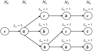
Figure 1: General trie-based dataset model of the sequential dataset in Table 1(c).

Foregoing the differences between application domains, the trie-based models of Yang et al. (2007); Pei et al. (2000); Lu and Ezeife (2003); Rizvee et al. (2020) are identical in their trie-based structure $(\mathcal{N},\mathcal{A})$. In fact, by definition of a trie, the trie-based dataset model $\mathcal{TD}$ of a sequential dataset $\mathcal{SD}$ is unique and of minimum-size in $(\mathcal{N},\mathcal{A})$. The distinguishing factor between different trie-based models of the literature is the additional labels defined for each node that are used to mine the trie. For example, the label set of the trie-based models used in web-access mining and their corresponding mining algorithms do not generalize to SPM, as they do not distinguish itemsets $\mathbb{I}_{i}^{j}\in\mathcal{S}_{i}$.

In order to model and mine sequential datasets in SPM, Rizvee et al. (2020) expand the label set $\mathcal{L}$ of each node $n\in\mathcal{N}$ by three additional labels. The first “event number” label is an integer that stores the position $j$ of itemset $\mathbb{I}_{i}^{j}:e_{n}\in\mathbb{I}_{i}^{j}$ of the prefix defined by path $({\bf{r}},\dots,n)$. The second “next links” label is a matrix of node pointers, where each row corresponds to an event $e\in\mathbb{E}$, and each column points to the first node $n^{\prime}:e_{n^{\prime}}=e$ for each path $(n,\dots,n^{\prime})$ spanning from node $n$. The last “parent info” label is a bitset that determines which events $e\in\mathbb{E}$ fall into the same itemset as event $e_{n}$ on the path $({\bf{r}},\dots,n)$. These labels are used in a tailored mining algorithm, TreeMiner, to mine all sequential patterns. Figure 2 shows the trie-based dataset model updated with next links and parent info for our running example.

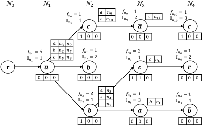
Figure 2: Trie-based dataset model used in TreeMiner (Rizvee et al., 2020). The matrix next to each node shows the next links, the vector under each node shows parent info, and the labels $\mathbb{I}$ give the event number labels.

TreeMiner traverses its trie-based dataset model using next links and mines sequential patterns using event number and patent info labels. Although these labels can enable faster traversal of the trie and SPM of the dataset, storing them at each node of the trie-based model is expensive in memory usage. In particular, the memory required to store the next link matrix and and parent info bitset labels at each node $n\in\mathcal{N}$ is bounded by $\mathcal{O}(|\mathbb{E}|^{2})$ and $\mathcal{O}(|\mathbb{E}|)$, respectively. This memory requirement decreases the effectiveness of the TreeMiner algorithm when the number of events $|\mathbb{E}|$ is large. Moreover, generating the next link label information introduces an computational overhead which may not be compensated by the faster traversal of the trie-based dataset model in the SPM algorithm. For a more memory-efficient SPM algorithm, we develop Sequential Data tries (SDTrie) and Binary Data tries (BDTries) that store a constant-size label set $\mathcal{L}$ at each node of a trie-based dataset model.

3 Sequential and Binary Data Tries for Memory Efficient SPM

An SDTrie is a trie-based model of the dataset with updated set of node labels $\mathcal{L}$. Specifically, in addition to event and frequency labels of general trie-based models, SDTries store at each node $n\in\mathcal{N}$ an itemset label $\mathbb{I}_{n}$ and an ancestor label $a_{n}$. The itemset label $\mathbb{I}_{n}$ is an integer identical to the event number label of Rizvee et al. (2020). The ancestor label $a_{n}$ is a pointer to a node, such that path $(a_{n},\dots,n)$ is the shortest path in $\mathcal{TD}$ that satisfies $\lVert e_{a_{n}}\rVert=\lVert e_{n}\rVert$. In other words, $a_{n}$ is the first prior node to node $n$ that has the same event label $\lVert e_{a_{n}}\rVert=\lVert e_{n}\rVert$. If no such node exists, the ancestor label is set to the root node $a_{n}={\bf{r}}$. Itemset and ancestor labels are the only required information to effectively mine sequential patterns from an SDTrie, and can be efficiently generated during construction as detailed in Algorithm 1. Example 3 demonstrates ancestor labels for our running example.

Example 3.

Consider the SDTrie model given in Figure 3(a). The ancestor label of node $n_{3}$ is $a_{n_{3}}=n_{1}$, as path $(n_{1},n_{2},n_{3})$ is the shortest path in the SDTrie such that $\lVert n_{1}\rVert=\lVert n_{3}\rVert=a$. Similarly, we have $a_{n_{6}}=n_{5}$ or $a_{n_{9}}=n_{1}$. The ancestor of node $n_{5}$ is $a_{n_{5}}={\bf{r}}$, as no prior node with the same event label $\lVert n_{5}\rVert=c$ exists on path $({\bf{r}},\dots,n_{5})$.

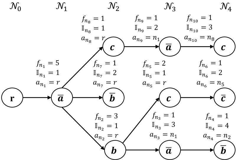
(a) SDTrie dataset model

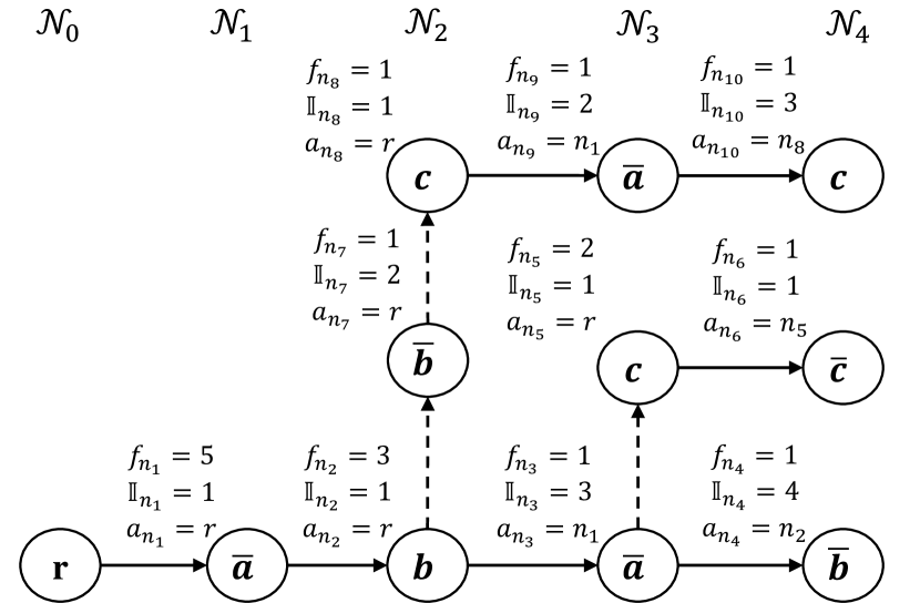
(b) BDTrie dataset model

Figure 3: The SDTrie and BDTrie models of the sequential dataset of Table 1(c). Sibling nodes are displayed by connected dashed arcs in the BDTrie.

Algorithm 1 Incremental Compilation of SDTries.

1:Initialize SDTrie with $\mathcal{N}:=\{{\bf{r}}\}$, $\mathcal{A}:=\emptyset$

2:Let $n={\bf{r}}$

3:for each $\mathcal{S}_{i}\in\mathcal{SD}$ do

4:     Let Anct$(e)={\bf{r}}$ for all $e\in\mathbb{E}$.

5:     Let ItmSet = 0.

6:     for $j\in\{1,\dots,|\mathcal{S}_{i}|\}$ do

7:         if there exists $(n,n^{\prime})\in\mathcal{A}$ such that $e_{n^{\prime}}=\mathcal{S}_{i}[j]$ then

8:              Update $f_{n}=f_{n}+1$,

9:              Let $n=n^{\prime}$.

10:         else

11:              Add $n^{\prime}:e_{n^{\prime}}=\mathcal{S}_{i}[j],f_{n^{\prime}}=1,a_{n^{\prime}}=\text{Anct}(\lVert\mathcal{S}_{i}[j]\rVert),\mathbb{I}_{n^{\prime}}=\text{ItmSet}$ to $\mathcal{N}_{j}$.

12:              Add $(n,n^{\prime})$ to $\mathcal{A}$.          

13:         if $\lVert\mathcal{S}_{i}[j]\rVert\neq\mathcal{S}_{i}[j]$ then

14:              Update ItmSet = ItmSet + 1.          

15:         Update Anct$(\lVert\mathcal{S}_{i}[j]\rVert)=n^{\prime}$.      

16:return SDTrie.

Although SDTries are more efficient than the trie-based models of the dataset in the SPM literature, we can still improve memory efficiency by redesigning their trie-based structure. In a trie-based model such as SDTries, a node $n\in\mathcal{TD}$ is connected to its children $n^{\prime}$ via arcs $(n,n^{\prime})$. Consequently, a node $n\in\mathcal{N}$ is required to store a pointer to each of its children. As the number of children for a node is unknown prior to the construction of a trie-based model, pointers to a node’s children must be stored via dynamic sized data structures. Unfortunately, dynamic data structures store overhead information which increases their memory requirement. Although this memory overhead is small and often overlooked, it can accumulate to higher memory usage in large-scale SPM as we show in our numerical results.

For better memory efficiency, we develop BDTries which are identical to SDTries in node and label sets $(\mathcal{N},\mathcal{L})$ but have a binary-trie data structure for arc set $\mathcal{A}$. In a BDTrie, a node $n$ has at most one child node $chl(n)$ and one sibling node $sib(n)$ which are used to model the entire set of its original children. Specifically, the first child of a node $n$ is connected to $n$ via arc $\left(n,chl(n)\right)$, and the remaining children are connected as contiguous siblings to child node $chl(n)$. Example 4 shows the child-sibling relationship of BDTries in our running example, and Algorithm 2 gives the incremental procedure of constructing BDTries.

Example 4.

Consider the BDTrie of our running example given in Figure 3(b). Nodes $n_{2},n_{7},n_{8}$ are all siblings and thus have the same parent $n_{1}$. This is indicated by the parent of the first sibling node $n_{2}$ which is the child node of $n_{1}$. Similarly, nodes $n_{3}$ and $n5$ are siblings with parent node $n_{2}$.

The challenge in using BDTries is determining how paths of the binary-trie represent sequences $\mathcal{S}_{i}\in\mathcal{SD}$. Recall that in trie-based models such as SDTries, there is a one-to-one correspondence between nodes of a path ${\mathbf{P}}=(n_{1},n_{2},\dots n_{j})$ and the events of its modeled sequences $\mathbf{TF}({\mathbf{P}})=\langle e_{n_{1}},e_{n_{2}},\dots,e_{n_{j}}\rangle$. This is no longer valid in BDTries, due to the presence of sibling arcs. To derive the sequence modeled by a path of a BDTries, we define a new transformation function $\mathbf{TF}^{B}({\mathbf{P}})$ as follows. For a path ${\mathbf{P}}=({\bf{r}},n_{1},\dots,n_{|{\mathbf{P}}|})$, the sequence modeled by ${\mathbf{P}}$ is given by $\mathbf{TF}^{B}({\mathbf{P}})=\langle e_{n_{1}},\dots,e_{n_{j}},\dots,e_{n_{|{\mathbf{P}}|}}\rangle$ where $e_{n_{j}}\in\mathbf{TF}^{B}({\mathbf{P}})$ if either $j=1$, $j=|{\mathbf{P}}|$, or $(n_{j},chl(n_{j}))\in{\mathbf{P}}$. In other words, the transformation function $\mathbf{TF}^{B}({\mathbf{P}})$ outputs the event of the first and last nodes $n_{1},n_{|{\mathbf{P}}|}\in{\mathbf{P}}$, and any node $n_{j}$ that is connected to its next immediate node $n_{j+1}$ via a child relationship in ${\mathbf{P}}$. Example 5 demonstrates this transformation function on our running example.

Example 5.

Consider the path ${\mathbf{P}}=({\bf{r}},n_{1},n_{2},n_{7},n_{8},n_{9})$ in the BDTrie of Figure 3(b). The transformation function gives $\mathbf{TF}^{B}({\mathbf{P}})=\langle e_{n_{1}},e_{n_{8}},e_{n_{9}}\rangle$. Here, nodes $n_{1},n_{9}$ are the first and last nodes in ${\mathbf{P}}$ and so events $e_{n_{1}},e_{n_{9}}$ are included in $\mathbf{TF}^{B}({\mathbf{P}})$. Event $e_{n_{8}}$ is also included in the transformation function due to the child relationship of arc $(n_{8},n_{9})\in{\mathbf{P}}$. Nodes $n_{2},n_{7}$ are excluded from the transformation as they are connected to their next immediate node in ${\mathbf{P}}$ via a sibling relationship.

Algorithm 2 Incremental Compilation of BDTries.

1:Initialize BDTrie with $\mathcal{N}:=\{{\bf{r}}\}$, $\mathcal{A}:=\emptyset$

2:Let $n={\bf{r}}$

3:for each $\mathcal{S}_{i}\in\mathcal{SD}$ do

4:     Let Anct$(e)={\bf{r}}$ for all $e\in\mathbb{E}$.

5:     Let ItmSet = 0.

6:     for $j\in\{1,\dots,|\mathcal{S}_{i}|\}$ do

7:         if node $n$ has a child $n^{\prime}=chl(n)$ then

8:              while $e_{n^{\prime}}\neq\mathcal{S}_{i}[j]$ and $n^{\prime}$ has a sibling node $n^{\prime\prime}=sib(n^{\prime})$ do

9:                  Let $n=n^{\prime}$,

10:                  Let $n^{\prime}=n^{\prime\prime}$.               

11:              if $e_{n^{\prime}}=\mathcal{S}_{i}[j]$ then

12:                  Update $f_{n^{\prime}}=f_{n^{\prime}}+1$, and set $n=n^{\prime}$.

13:              else

14:                  Add $n^{\prime}:e_{n^{\prime}}=\mathcal{S}_{i}[j],f_{n^{\prime}}=1,a_{n^{\prime}}=\text{Anct}(\lVert\mathcal{S}_{i}[j]\rVert),\mathbb{I}_{n^{\prime}}=\text{ItmSet}$ to $\mathcal{N}_{j}$.

15:                  Add sibling arc $(n,n^{\prime})$ to $\mathcal{A}$.               

16:         else

17:              Add $n^{\prime}:e_{n^{\prime}}=\mathcal{S}_{i}[j],f_{n^{\prime}}=1,a_{n^{\prime}}=\text{Anct}(\lVert\mathcal{S}_{i}[j]\rVert),\mathbb{I}_{n^{\prime}}=\text{ItmSet}$ to $\mathcal{N}_{j}$.

18:              Add child arc $(n,n^{\prime})$ to $\mathcal{A}$.          

19:         if $\lVert\mathcal{S}_{i}[j]\rVert\neq\mathcal{S}_{i}[j]$ then

20:              Update ItmSet = ItmSet + 1.          

21:         Update Anct$(\lVert\mathcal{S}_{i}[j]\rVert)=n^{\prime}$.      

22:return BDTrie.

The advantage of BDTries over SDTries and other trie-based models is that the number of arcs spanning from a node $n\in\mathcal{N}$ of a BDTrie is constant and binary. Dynamic data structures are thus no longer required to be stored at each node of the trie-based model, leading to higher memory efficiency. As we show in our numerical tests, BDTries consistently outperform SDTries and TreeMiner on memory usage as well as computational time in the mining algorithm.

3.1 Mining SDTries and BDTries

Given a sequential dataset, the SPM task involves finding all patterns $\mathcal{P}$ such that $supp(\mathcal{P})\geq\theta\times N$. This is generally done in recursive fashion, where at each iteration a pattern $\mathcal{P}$ is extended by an event $e\in\bar{\mathbb{E}}$ to $\langle\mathcal{P},e\rangle$, and checked to satisfy $supp(\langle\mathcal{P},e\rangle)\geq\theta\times N$. A Pattern extension can be categorized into an itemset extension or a sequence extension. In an itemset extension, a pattern $\mathcal{P}$ is extended to $\langle\mathcal{P},e\rangle$ and satisfies $\lVert e\rVert=e$. In other words, event $e$ is added to the last itemset of pattern $\mathcal{P}$. In a sequence extension, a pattern is extended to $\langle\mathcal{P},\bar{e}\rangle$ and has $\lVert\bar{e}\rVert=e$. In other words, event $\bar{e}$ extends pattern $\mathcal{P}$ by a new itemset $\mathbb{I}=\{\bar{e}\}$.

For tabular-based datasets, the mining algorithm starts with frequent patterns containing a single event, that is, frequent events $\bar{e}\in\bar{\mathbb{E}}$ (note that the first event of any pattern must be a transformed event $\bar{e}$), and maintains a tuple of pattern-position pairs $\left(\mathcal{P},\{(i,j)\}_{i\in\{1,\dots,N\}}\right)$. Here, a position pair $(i,j)$ specifies a minimum-size prefix $\mathcal{\bar{S}}_{i}=\langle\mathcal{S}_{i}[1],\dots,\mathcal{S}_{i}[j]\rangle$ that contains $\mathcal{P}$ as a subsequence. The prefix is minimum-size in that no other prefix $\mathcal{\bar{S}}_{i}^{\prime}:|\mathcal{\bar{S}}_{i}^{\prime}|<|\mathcal{\bar{S}}_{i}|,\mathcal{P}\sqsubseteq\mathcal{\bar{S}}_{i}^{\prime}$ exists for sequence $\mathcal{S}_{i}$. At each iteration, the mining algorithm takes a tuple $(\mathcal{P},\{(i,j)\}_{i\in\{1,\dots,N\}})$ and attempts to extend $\mathcal{P}$ by a single scan of events in $\langle\mathcal{S}_{i}[j],\dots,\mathcal{S}_{i}[|\mathcal{S}_{i}|]\rangle$. If $\mathcal{S}_{i}[j^{\prime}]$ is the first occurrence of an event $e$ in $\langle\mathcal{S}_{i}[j],\dots,\mathcal{S}_{i}[|\mathcal{S}_{i}|]\rangle$, position pair $(i,j^{\prime})$ is added to the tuple of pattern $\langle\mathcal{P},e\rangle$. If an event $e\in\bar{\mathbb{E}}$ is found in more than $\theta\times N$ of such sequences, then $\langle\mathcal{P},e\rangle$ is a frequent pattern. This algorithm is commonly known as the pseudo-projection algorithm (Han et al., 2001).

Mining SDTries or BDTries is done by traversing their paths in DFS manner. Similar to pseudo-projection on tabular-based models, our mining algorithm maintains a set of pattern-node pairs $(\mathcal{P},\mathcal{N}(\mathcal{P}))$. Here, set $\mathcal{N}(\mathcal{P})$ contains the terminal nodes of all paths ${\mathbf{P}}\in\mathcal{TD}$ that model a minimum-sized prefix $\mathbf{TF}({\mathbf{P}}):\mathcal{P}\sqsubseteq\mathbf{TF}({\mathbf{P}})$, or in the case of BDTries $\mathbf{TF}^{B}({\mathbf{P}}):\mathcal{P}\sqsubseteq\mathbf{TF}^{B}({\mathbf{P}})$. Following the logic of prefix-projection algorithms (Han et al., 2000), minimum-sized prefixes are found by finding the first occurrence of events $e\in\bar{\mathbb{E}}$ in the sub-tries rooted at nodes $n\in\mathcal{N}(\mathcal{P})$. If $\sum_{n\in\mathcal{N}(\langle\mathcal{P},e\rangle)}f_{n}\geq\theta\times N$ then $\langle\mathcal{P},e\rangle$ is a frequent pattern. The main task of mining trie-based datasets thus involves effectively finding sets $\mathcal{N}(\mathcal{P})$. That is, determining whether a traversed node $n$ is the first occurrence of event $e_{n}$ during the mining algorithm. Theorem 6 provides a necessary and sufficient condition using itemset and ancestor labels.

Theorem 6.

Let node $n^{\prime}\in\mathcal{N}$ be a node traversed when searching the sub-trie rooted at a node $n\in\mathcal{N}(\mathcal{P})$. Node $n^{\prime}$ belongs to set $\mathcal{N}\left(\langle\mathcal{P},e_{n^{\prime}}\rangle\right)$ if and only if:

• For a sequence extension $\langle\mathcal{P},\bar{e}_{n^{\prime}}\rangle$ we have $\mathbb{I}_{a_{n^{\prime}}}\leq\mathbb{I}_{n}$,

• For an itemset extension $\langle\mathcal{P},e_{n^{\prime}}\rangle$ we have either:

  • $\mathbb{I}_{a_{n^{\prime}}}<\mathbb{I}_{n}$ or,

  • For all nodes $n^{\prime\prime}$ on the path ${\mathbf{P}}=(n,\dots,n^{\prime})$, $n^{\prime\prime}\notin\mathcal{N}\left(\langle\mathcal{P},e_{n^{\prime}}\rangle\right)$.

Proof.

By definition, node $n^{\prime}$ belongs to $\mathcal{N}\left(\langle\mathcal{P},e_{n^{\prime}}\rangle\right)$ if and only if it is the first occurrence of event $e_{n^{\prime}}$ in the path ${\mathbf{P}}=(n,\dots,n^{\prime})$. The proof thus reduces to proving that node $n^{\prime}$ is the first occurrence of event $e_{n^{\prime}}$ on the path $(n,\dots,n^{\prime})$.

Consider the case where $\mathbb{I}_{a_{n^{\prime}}}<\mathbb{I}_{n}$, that is, when $a_{n^{\prime}}$ occurs prior to node $n$. The path from the root node to node $n^{\prime}$ is thus of the form $({\bf{r}},\dots,a_{n^{\prime}},\dots,n,\dots,n^{\prime})$. By definition of ancestor labels, path $(a_{n^{\prime}},\dots,n^{\prime})$ is the shortest path in the trie such that $\lVert e_{a_{n^{\prime}}}\rVert=\lVert e_{n^{\prime}}\rVert$. Therefore, $n^{\prime}$ is the first occurrence of event $e_{n^{\prime}}$ on path $(n,\dots,n^{\prime})$.

Consider the case where $\mathbb{I}_{a_{n^{\prime}}}=\mathbb{I}_{n}$. The path from the root node to node $n^{\prime}$ is either of the form $({\bf{r}},\dots,a_{n^{\prime}},\dots,n,\dots,n^{\prime})$ or of the form $({\bf{r}},\dots,n,\dots,a_{n^{\prime}},\dots,n^{\prime})$. In the former, as discussed above, node $n^{\prime}$ is the first occurrence of event $e_{n^{\prime}}$ on path $(n,\dots,n^{\prime})$. In the latter, $n^{\prime}$ is the second occurrence of event $e_{n^{\prime}}$ on path $(n,\dots,n^{\prime})$, after node $a_{n^{\prime}}$. However, as nodes $n$ and $a_{n^{\prime}}$ model events from the same itemset, $a_{n^{\prime}}$ cannot be used for a sequence extension of pattern $\mathcal{P}$. This means Node $n^{\prime}$ is the first occurrence of event $e_{n^{\prime}}$ on path $(n,\dots,n^{\prime})$ that can be used for a sequence extension, but not an itemset extension.

Lastly, assume by contradiction that $\exists n^{\prime\prime}\in\mathcal{N}\left(\langle\mathcal{P},e_{n^{\prime}}\rangle\right)$ on the path $(n,\dots,n^{\prime})$, and that node $n^{\prime}$ is the first occurrence of event $e_{n^{\prime}}$. This trivially means that $n^{\prime\prime}$ (and not $n^{\prime}$) is the first occurrence of event $e_{n^{\prime\prime}}=e_{n^{\prime}}$ on the path $(n,\dots,n^{\prime})$, a contradiction. ∎

At each iteration, our mining algorithm takes a tuple $(\mathcal{P},\mathcal{N}(\mathcal{P}))$ and attempts to extend $\mathcal{P}$ by a single scan of the sub-tries rooted at nodes $n\in\mathcal{N}(\mathcal{P})$. For a node $n\in\mathcal{N}(\mathcal{P})$, the search is performed in two phases. In the first phase, we search the paths rooted at node $n$ up until the first node $n^{\prime}:\lVert e_{n^{\prime}}\rVert\neq e_{n^{\prime}}$, that is, a transformed event $\bar{e}_{n^{\prime}}$. Note that such paths $(n,\dots,n^{\prime})$ model the events of the same itemset, and no two events can be the same within the same itemset. Therefore, any node $n^{\prime\prime}\in(n,\dots,n^{\prime})$ corresponds to the first occurrence of an event $e_{n^{\prime\prime}}$ and already satisfies the conditions of Theorem 6 for an itemset extension. Moreover, nodes $n^{\prime}$ correspond to the first occurrence of an event $\bar{e}_{n^{\prime}}$ and represent a valid sequence extension. In the second phase, we mine the sub-tries rooted at nodes $n^{\prime}$ and determine valid sequence and itemset extensions using the conditions of Theorem 6. The complete mining algorithm is given in Algorithm 3, and exemplified in Example 7.

Algorithm 3 SPM of SDTrie and BDTrie Dataset Models.

1:Initialize pattern-node pairs $\left\{\left(\mathcal{P},\mathcal{N}(\mathcal{P})\right):=\mathcal{P}=\langle\bar{e}\rangle,\;\forall\bar{e}\in\bar{\mathbb{E}}:supp(\bar{e})\geq\theta\times N\right\}$.

2:for each pair $(\mathcal{P},\mathcal{N}(\mathcal{P}))$ do

3:     Let $\mathcal{N}\left(\langle\mathcal{P},e\rangle\right)=\emptyset$ for all $e\in\bar{\mathbb{E}}$, and $j=\max_{j}:\lVert\mathcal{P}[j]\rVert\neq\mathcal{P}[j]$.

4:     for each $n\in\mathcal{N}(\mathcal{P})$ do

5:         Initialize DFS queues $Q^{1}_{\mathcal{N}}=\langle n\rangle$, $Q^{2}_{\mathcal{N}}=\langle\rangle$, $Q^{2}_{\mathbb{I}}=\langle\rangle$.

6:         while $Q^{1}_{\mathcal{N}}$ is nonempty do

7:              Take $n^{\prime}$ from the front of queue $Q^{1}_{\mathcal{N}}$.

8:              for each child (or child-sibling) node $n^{\prime\prime}$ of node $n^{\prime}$ do

9:                  if $\lVert e_{n^{\prime\prime}}\rVert=e_{n^{\prime\prime}}$ then

10:                       Add node $n^{\prime\prime}$ to $\mathcal{N}\left(\langle\mathcal{P},e_{n^{\prime\prime}}\rangle\right)$ as an itemset extension,

11:                       Add node $n^{\prime\prime}$ to the front of queue $Q^{1}_{\mathcal{N}}$.

12:                  else

13:                       Add node $n^{\prime\prime}$ to $\mathcal{N}\left(\langle\mathcal{P},\bar{e}_{n^{\prime\prime}}\rangle\right)$ as a sequence extension,

14:                       Add node $n^{\prime\prime}$ to the front of queue $Q^{2}_{\mathcal{N}}$.

15:                       if $e_{n^{\prime\prime}}=\mathcal{P}[j]$ then

16:                           Add 1 to the front of queue $Q^{2}_{\mathbb{I}}$.

17:                       else

18:                           Add 0 to the front of queue $Q^{2}_{\mathbb{I}}$.                                                                 

19:         while $Q^{2}_{\mathcal{N}}$ is nonempty do

20:              Take $n^{\prime}$ from the front of queue $Q^{2}_{\mathcal{N}}$, and integer $k$ from front of queue $Q^{2}_{\mathbb{I}}$.

21:              for each child (or child-sibling) node $n^{\prime\prime}$ of node $n^{\prime}$ do

22:                  if $\lVert e_{n^{\prime\prime}}\rVert=e_{n^{\prime\prime}}$ then

23:                       if $k=|\mathcal{P}|-j$ and conditions of Theorem 6 are satisfied then

24:                           Add node $n^{\prime\prime}$ to $\mathcal{N}\left(\langle\mathcal{P},e_{n^{\prime\prime}}\rangle\right)$ as an itemset extension.                        

25:                       if Conditions of Theorem 6 are satisfied then

26:                           Add node $n^{\prime\prime}$ to $\mathcal{N}\left(\langle\mathcal{P},\bar{e}_{n^{\prime\prime}}\rangle\right)$ as a sequence extension.                        

27:                       Add node $n^{\prime\prime}$ to the front of queue $Q^{2}_{\mathcal{N}}$.

28:                       if $k<|\mathcal{P}|-j$ and $e_{n^{\prime\prime}}=\mathcal{P}[k+j]$ then

29:                           Add k + 1 to the front of queue $Q^{2}_{\mathbb{I}}$.

30:                       else

31:                           Add k to the front of queue $Q^{2}_{\mathbb{I}}$.                        

32:                  else

33:                       if conditions of Theorem 6 are satisfied then

34:                           Add node $n^{\prime\prime}$ to $\mathcal{N}\left(\langle\mathcal{P},\bar{e}_{n}\rangle\right)$ as a sequence extension.                        

35:                       Add node $n^{\prime\prime}$ to the front of queue $Q^{2}_{\mathcal{N}}$.

36:                       if $e_{n^{\prime\prime}}=\mathcal{P}[j]$ then

37:                           Add 1 to the front of queue $Q^{2}_{\mathbb{I}}$.

38:                       else

39:                           Add 0 to the front of queue $Q^{2}_{\mathbb{I}}$.                                                                      

40:     for each $e\in\bar{\mathbb{E}}$ do

41:         if $\sum_{n\in\mathcal{N}\left(\langle\mathcal{P},e\rangle\right)}f_{n}\geq\theta\times N$ then

42:              Add $\left(\langle\mathcal{P},e\rangle,\mathcal{N}\left(\langle\mathcal{P},e\rangle\right)\right)$ to the set of pattern-node pairs.               

43:return Set of frequent patterns $\mathcal{P}:\sum_{n\in\mathcal{N}\left(\mathcal{P}\right)}f_{n}\geq\theta\times N$.

Example 7.

SPM over the SDTrie model depicted in Figure 3(a) initializes with pattern-node pairs $(\langle\bar{a}\rangle,\{n_{1}\}),(\langle\bar{b}\rangle,\{n_{2},n_{7}\}),(\langle\bar{c}\rangle,\{n_{5},n_{8}\})$. The mining algorithm takes a pattern-node pair, for example, $(\langle\bar{a}\rangle,\{n_{1}\})$, and in the first phase searches the sub-trie rooted at node $n_{1}$ to find the first occurrence of events $\bar{e}\in\bar{\mathbb{E}}$, that is, nodes $n_{3},n_{6},n_{7},n_{9}$. This search results in finding pattern-node pairs $\left(\langle\bar{a},\bar{a}\rangle,\{n_{3},n_{9}\}),(\langle\bar{a},b\rangle,\{n_{2}\}),(\langle\bar{a},\bar{b}\rangle,\{n_{7}\}),(\langle\bar{a},c\rangle,\{n_{5},n_{8}\}),(\langle\bar{a},\bar{c}\rangle,\{n_{6}\})\right)$. In the second phase, search is initiated from nodes $n_{3},n_{6},n_{7},n_{9}$. Searching the sub-trie rooted at node $n_{3}$ traverses node $n_{4}$, which has $e_{n_{4}}=\bar{a}$ and thus corresponds to a sequence extension. Furthermore, we have $\mathbb{I}_{n_{1}}=\mathbb{I}_{a_{n_{4}}}$ which satisfies the sequence extension condition of Theorem 6. The corresponding pattern-node pair is thus updated to $(\langle\bar{a},\bar{b}\rangle,\{n_{4},n_{7}\})$. Searching the sub-trie rooted at node $n_{9}$ traverses node $n_{10}$, which has $e_{n_{10}}=c$ and can correspond to an itemset or a sequence extension. We have $\mathbb{I}_{n_{1}}=\mathbb{I}_{a_{n_{10}}}$, which violates the itemset extension condition of Theorem 6, but satisfies its sequence extension condition. The corresponding pattern-node pair is thus updated to $\left(\langle\bar{a},\bar{c}\rangle,\{n_{6},n_{10}\})\right)$. The support of any pattern is given by $\sum_{n\in\mathcal{N}(\mathcal{P})}f_{n}$. For example, pattern $\langle\bar{a},\bar{a}\rangle$ has support $supp(\langle\bar{a},\bar{c}\rangle)=f_{n_{5}}+f_{n_{10}}=3$. The process is repeated for any frequent pattern-node pair until all found pairs are verified.

Mining a pattern $\mathcal{P}$ from an SDTrie or BDTrie dataset model is $|\mathcal{N}(\mathcal{P})|/\sum_{n\in\mathcal{N}(\mathcal{P})}f_{n}$ times more memory efficient than mining $\mathcal{P}$ from a tabular-based dataset as proved in Proposition 8. In the worst-case, we have $f_{n}=1,\forall n\in\mathcal{N}(\mathcal{P})$, and the mining algorithms store the same number of position pairs $|\mathcal{N}(\mathcal{P})|=\sum_{n\in\mathcal{N}(\mathcal{P})}f_{n}$. Therefore, our mining algorithm is in the worst-case as memory efficient as mining a tabular-based model. Note that this efficiency concerns only the mining algorithm and does not include the memory savings of storing a trie-based model compared to a tabular-based dataset detailed in the next section.

Proposition 8.

Mining a frequent pattern $\mathcal{P}$ from an SDTrie or BDTrie via Algorithm 3 is $\mathcal{O}(|\mathcal{N}(\mathcal{P})|/\sum_{n\in\mathcal{N}(\mathcal{P})}f_{n})$ times more memory efficient than mining $\mathcal{P}$ from a tabular-based dataset model via pseudo-projection.

Proof.

Mining SDTries or BDTries involves storing $|\mathcal{N}(\mathcal{P})|$ pointers to nodes at each iteration, while mining a tabular-based dataset involves storing $\sum_{n\in\mathcal{N}(\mathcal{P})}f_{n}$ pairs of integers. For any pattern $\mathcal{P}$, mining a trie-based dataset is thus $\mathcal{O}(|\mathcal{N}(\mathcal{P})|/\sum_{n\in\mathcal{N}}f_{n})$ times more memory efficient than mining its tabular-based counterfeit. ∎

3.2 Space Complexity of SDTries and BDTries

This section analyzes the worst-case space complexity of SDTries and BDTries. For brevity, and without loss of generality, we assume that events $e$ are represented by positive integers, events $\bar{e}$ are represented by negative integers, and $|\mathbb{E}|,M\leq N$. For a thorough analysis of large-size datasets, we further consider that representing any integer $j$ has $\log(|j|)$ space complexity (Papadimitriou and Steiglitz, 1998). We later discuss the relaxation of this consideration, and assume constant memory consumption for reasonably-sized integers.

The size of a sequential dataset $\mathcal{SD}$ is in the order of its total number of entries, that is, $|\mathcal{SD}|:=\mathcal{O}\left(\sum_{i=1}^{N}|\mathcal{S}_{i}|\right)$. The worst-case space complexity of a tabular model $|\mathcal{SD}|$ is thus bounded by $\mathcal{O}\left(NM\log(|\mathbb{E}|)\right)$. The size of an SDTrie or BDTrie is in the order of their total number of nodes, that is, $\mathcal{O}\left(|\mathcal{N}|\right)$. It thus suffices to determine the space complexity of a single node $n\in\mathcal{N}$, given in Lemma 9, and the total number of nodes in a trie-based model, given in Lemma 10.

Lemma 9.

The space complexity an SDTrie node is bounded by $\mathcal{O}\left(|\mathbb{E}|+\log(N)\right)$; and the space complexity a BDTrie node is bounded by $\mathcal{O}\left(\log(N)\right)$.

Proof.

A node $n$ in an SDTrie stores integer values $f_{n}$, $e_{n}$, $\mathbb{I}_{n}$, a pointer $a_{n}$, and one pointer for each of its children. Each integer can be at most $N$ and takes $\mathcal{O}\left(\log(N)\right)$ space. By definition, a node $n\in\mathcal{N}$ has at most $|\bar{\mathbb{E}}|=2|\mathbb{E}|$ children. The space complexity of an SDTrie node is thus $\mathcal{O}\left(|\mathbb{E}|+\log(N)\right)$.

The space complexity of a node $n$ in a BDTrie is similar to a node $n$ in an SDTrie, with the exception of having one pointer per its child and sibling nodes instead of the $2|\mathbb{E}|$ pointers for its children. The space complexity of a BDTrie node $n$ is thus $\mathcal{O}\left(\log(N)\right)$. ∎

Lemma 10.

The total number of nodes in a trie-based model is bounded by $\mathcal{O}\left(\min\{N,|\mathbb{E}|^{M}\}M\right)$

Proof.

By definition, a node $n\in\mathcal{N}$ has at most $2|\mathbb{E}|$ children. The maximum number of children for a layer $\mathcal{N}_{j}$ is thus $\left(2|\mathbb{E}|\right)^{|\mathcal{N}_{j}|}$. As $|\mathcal{N}_{0}|=1$, the maximum number of nodes for any layer is $\left(2|\mathbb{E}|\right)^{M}$. On the other hand, we can have at most $N$ nodes at any layer of a trie-based model of a sequential dataset, where each sequence $\mathcal{S}_{i}\in\mathcal{SD}$ is represented by exactly one path. The maximum number of nodes for all $M+1$ number of layers in a trie-based model is thus bounded by $\mathcal{O}\left(\min\{N,|\mathbb{E}|^{M}\}M\right)$ ∎

Using Lemmas 9 and 10, the worst-case space complexity of SDTries and BDTries is given by Theorem 11.

Theorem 11.

The worst-case space complexity of SDTries and BDTries is bounded by
$\mathcal{O}\left(\min\{N,|\mathbb{E}|^{M}\}M(|\mathbb{E}|+\log(N))\right)$ and $\mathcal{O}\left(\min\{N,|\mathbb{E}|^{M}\}M\log(N)\right)$, respectively.

Proof.

The proof trivially follows from Lemmas 9 and 10. ∎

In the best case for SDTries and BDTries, we have $|\mathbb{E}|=1$ and a space complexity in the order of $M\log(N)$, leading to $N/\log(N)$ times more efficient memory consumption than a tabular model. In the worst case, SDTries and BDTries use $\left(|\mathbb{E}|+\log(N)\right)/\log(|\mathbb{E}|)$ and $\log(N)/\log(|\mathbb{E}|)$ times more memory to store the trie-based model of the dataset, respectively.

In practice, reasonably sized integer values consume constant memory. In such cases, the space complexity of tabular models reduces to $\mathcal{O}\left(NM\right)$, and the space complexity of SDTries and BDTries reduce to $\mathcal{O}\left(\min\{N,|\mathbb{E}|^{M}\}M|\mathbb{E}|\right)$ and $\mathcal{O}\left(\min\{N,|\mathbb{E}|^{M}\}M\right)$, respectively. This means that, asymptotically, BDTries are never larger than tabular-based dataset models and in the worst-case grow with the same rate in $N,M$. Moreover, when bounded by $\mathcal{O}(M|\mathbb{E}|^{M})$, SDTries and BDTries practically enjoy a capped memory requirement despite an arbitrary increase in $N$. This is especially significant for large-size applications of SPM where $N$ is typically orders of magnitudes larger than both $|\mathbb{E}|$ and $M$. For such applications, SDTries and BDTries are expected to be orders of magnitude more memory efficient than a tabular model of the dataset. We indeed observe such savings in our numerical results.

4 Numerical Results

For our numerical tests we evaluate the effect of different dataset models on the performance of state-of-the-art mining algorithms in large-scale SPM. We emphasize that we do not seek to improve upon any specialized SPM algorithm. As previously discussed, our techniques and models are generic and can be applied to, or enhanced by, the many advancements made in the rich literature of SPM. We thus focus our attention to the two algorithms of PrefixSpan by Han et al. (2001) which forms the basis of many state-of-the-art tabular-based prefix-projection algorithms, and TreeMiner (Rizvee et al., 2020) which is the state-of-the-art in trie-based models for SPM.

We start by describing our datasets and experimental setup in §4.1 and perform our numerical tests in three phases. We first examine in §4.2 the effect of dataset flattening techniques on the PrefixSpan algorithm. We then evaluate in §4.3 the effect of support-based filtering on the best performing PrefixSpan algorithm in §4.2, and the TreeMiner algorithm. Lastly, we conclude our numerical tests in §4.4 by comparing SDTries and BDTries to the best performing tabular-based and trie-based algorithms found in §4.3.

4.1 Data and Experimental Setup

Table 3: Five real-life datasets and their attributes.

Dataset	$N$	$|\mathbb{E}|$	$M$	$avg(|\mathcal{S}|)$*	$max(|\mathbb{I}|)$	$avg(|\mathbb{I}|)$*	$\sum_{\mathcal{S}\in\mathcal{SD}}|\mathcal{S}|$
Twitch	15,524,308	790,100	456	30.3	170	1.2	469,655,703
Amazon	42,796,890	28	1,081	3.7	23	1.3	159,409,747
Spotify	124,950,054	5	20	2.4	5	1.1	294,302,842
Kosarak	990,002	41,270	2,498	8.1	1	1	8,019,015
MSNBC	989,818	17	14,795	4.8	1	1	4,698,794
*Denotes average value.

We perform our numerical tests over five large-size real-life datasets detailed in Table 3. Two of our datasets, Kosarak and MSNBC, are benchmark click-stream instances in SPM (Fournier-Viger et al., 2016), despite the fact that the literature often considers a much smaller subset of these instances. The remaining three datasets are larger and more recent datasets that demonstrate the need for scalability in SPM. The Twitch dataset (Rappaz et al., 2021) is a dataset of users consuming streaming content on the live streaming platform Twitch. Here, events $e\in\mathbb{E}$ are defined as a unique streamer, and consecutive streamers watched by a user form a sequence $\mathcal{S}_{i}\in\mathcal{SD}$. Two consecutive events are assumed to be in the same itemset if they are visited by the user within a one hour time frame. The Amazon dataset (Ni et al., 2019) is a collection of user reviews for items purchased on the E-commerce platform Amazon. We transform the data into a sequential dataset by assuming that reviews were made within a month of their product purchase, and thus act as a substitute for a product purchase event. An event $e\in\mathbb{E}$ is defined to be the category of the product purchased by a user. Products purchased within the same month are considered to be in the same itemset. The Spotify dataset (Brost et al., 2019) is a collection of user music consumption on the media streaming platform Spotify. Events $e\in\mathbb{E}$ are considered to be the time-signature (refer to Brost et al. (2019) for definition of time-signature) of consumed media. Events are considered to be in different itemsets if a context switch (refer to Brost et al. (2019) for definition of a context switch) occurs between them.

All algorithms are coded in C++ and executed on a PC with an Intel Xeon processor W-2255, 128GB of memory, and Ubuntu 20.04.1 as the operating system. We limit all tests to use one core of the CPU. All instances are mined under a minimum support threshold $\theta\in\{10\%,8\%,6\%,4\%,2\%,0.5\%\}$.

4.2 Effects of Dataset Flattening Techniques

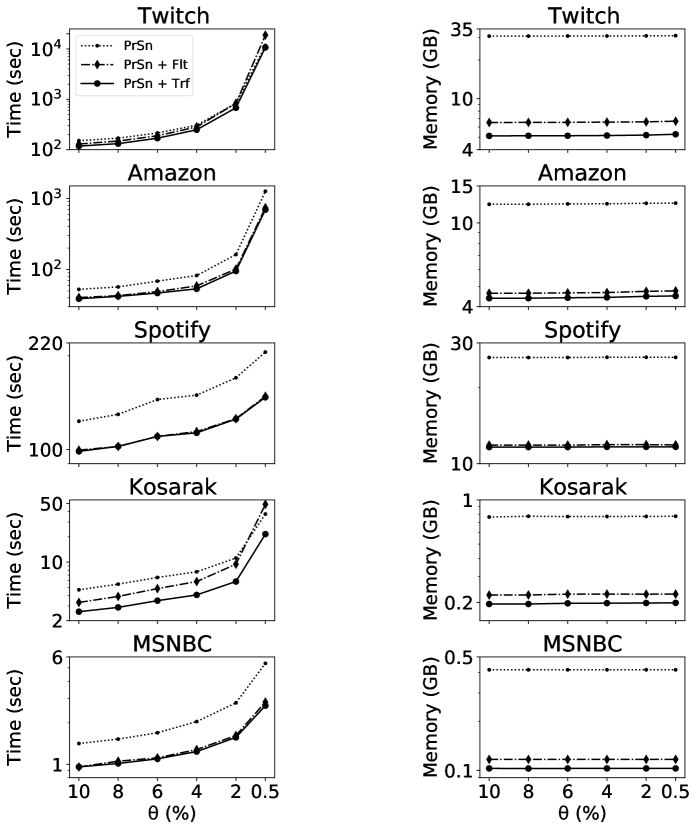
Figure 4: Total computational time and peak memory usage of the PrefixSpan algorithm on datasets without flattening (PrSn), flattened via separating literals (PrSn + Flt), and flattened via transformed events (PrSn + Trf).

Figure 4 gives the total computational time and peak memory usage of the PrefixSpan algorithm under the three different dataset flattening techniques: 1. The original PrefixSpan algorithm without any dataset flattening technique (PrSn), 2. PrefixSpan on datasets flattened via separating literals (PrSn + Flt), and 3. PrefixSpan on datasets flattened via transformed events (PrSn + Trf).

Results show considerable improvements in memory usage and faster mining when flattening techniques are used compared to the original PrefixSpan algorithm. Flattening the dataset by transformed events is slightly more effective compared to using a separating literal, in particular, when sequences are longer on average such as in the Twitch dataset. For our next set of numerical tests, we thus use PrefixSpan on a flattened dataset via transformed events (PrSn + Trf) as the best performing tabular-based SPM algorithm.

4.3 Effects of Support-based Filtering

While SDTries and BDTries include dataset flattening and support-based filtering in their design, support-based filtering of the dataset is not performed in the PrefixSpan and TreeMiner algorithms. For a fairer comparison to SDTries and BDTries, we first test whether support-based filtering can benefit such state-of-the-art algorithms on total computational time and peak memory usage.

Table 4: Dataset attributes with support-based filtering.

Dataset	$\theta$ (%)	$\theta\times N$	$N$	$|\mathbb{E}|$	$M$	$avg(|\mathcal{S}|)$	$max(|\mathbb{I}|)$	$avg(|\mathbb{I}|)$	$\sum_{\mathcal{S}\in\mathcal{SD}}|\mathcal{S}|$
Twitch	10	1,552,431	4,554,694	3	47	3.9	3	1	17,623,769
	8	1,241,945	4,554,694	3	47	3.9	3	1	17,623,769
	6	931,458	5,950,368	7	65	4.5	5	1	27,069,846
	4	620,972	6,863,408	14	100	5.9	6	1	40,168,541
	2	310,486	9,295,847	49	161	8.1	12	1.1	75,339,296
	0.5	77,622	12,813,843	356	234	13.7	44	1.1	175,978,595
Amazon	10	4,279,689	36,456,711	7	551	3.1	7	1.2	111,243,567
	8	3,423,751	39,182,652	10	690	3.3	10	1.2	128,803,295
	6	2,567,813	40,530,143	13	891	3.5	13	1.2	141,263,553
	4	1,711,876	41,547,233	15	914	3.6	15	1.3	148,453,509
	2	855,938	42,364,478	19	1,033	3.7	19	1.3	155,147,709
	0.5	213,984	42,769,800	26	1,078	3.7	23	1.3	159,195,936
Spotify	10	12,495,005	124,943,444	3	20	2.3	3	1.1	284,947,678
	8	9,996,004	124,943,444	3	20	2.3	3	1.1	284,947,678
	6	7,497,003	124,944,864	4	20	2.4	4	1.1	293,972,062
	4	4,998,002	124,944,864	4	20	2.4	4	1.1	293,972,062
	2	2,499,001	124,944,864	4	20	2.4	4	1.1	293,972,062
	0.5	624,750	124,944,864	4	20	2.4	4	1.1	293,972,062
Kosarak	10	99,000	843,959	4	4	1.9	1	1	1,612,992
	8	79,200	854,232	6	6	2.1	1	1	1,788,488
	6	59,400	882,799	10	10	2.3	1	1	2,074,053
	4	39,600	892,085	13	13	2.5	1	1	2,208,696
	2	19,800	909,195	27	25	2.8	1	1	2,559,408
	0.5	4,950	931,167	156	145	3.9	1	1	3,617,201
MSNBC	10	98,982	816,098	7	14,795	3.8	1	1	3,062,259
	8	79,185	921,804	10	14,795	4.3	1	1	4,003,886
	6	59,389	961,805	11	14,795	4.4	1	1	4,220,011
	4	39,593	981,468	13	14,795	4.5	1	1	4,448,588
	2	19,796	988,592	15	14,795	4.7	1	1	4,656,573
	0.5	4,949	989,562	16	14,795	4.7	1	1	4,673,545

Table 4 shows the change in attributes of our considered datasets with support-based filtering. Note that for correct SPM over filtered datasets $\theta\times N$ is calculated based on the original number of sequences $N$ given in Table 3. Results show that support-based filtering often results in considerable reduction of the dataset size, particularly for higher values of $\theta$. Figure 5 gives the results of SPM over filtered datasets for the PrefixSpan + Trf and TreeMiner algorithms. Results show that support-based filtering lowers memory usage in almost all instances, particularly for higher values of $\theta$. Memory savings are higher for datasets with a higher number of events $|\mathbb{E}|$, for example, in the Twitter and Kosarak instances. Such datasets have higher potential of containing infrequent events $e:supp(e)<\theta\times N$, and thus a higher potential for space saving via support-based filtering. Support-based filtering is especially beneficial for TreeMiner, often leading to orders of magnitude lower memory requirements. In fact, without support-based filtering, TreeMiner cannot fit the Twitch dataset in 128GB of memory.

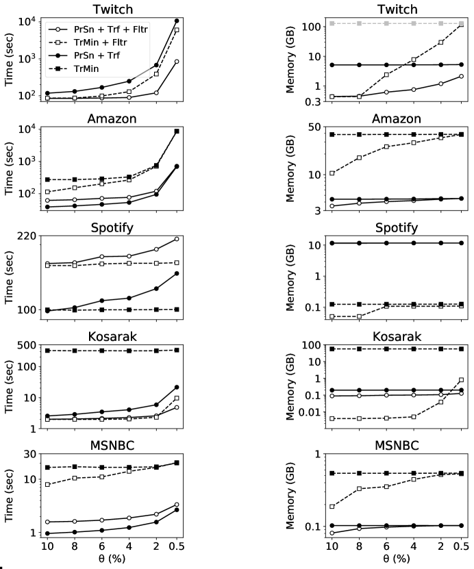
Figure 5: Total computational time and peak memory usage of PrefixSpan with transformed events (PrSn + Trf), PrefixSpan with transformed events and support-based filtering (PrSn + Trf + Fltr), TreeMiner (TrMin), and TreeMiner with support-based filtering (TrMin + Fltr).

In terms of computation time, support-based filtering adds an overhead of a single dataset scan in SPM. This overhead is mostly compensated with a faster mining algorithm due to the smaller search space, such as in the Twitch and Kosarak datasets. For example, PrefixSpan is an order of magnitude faster when support-based filtering is performed on the twitch dataset with $\theta=0.5\%$. Support-based filtering may lead to higher overall mining time when the number of infrequent events $e:supp(e)<\theta\times N$ is low, e.g, in the Spotify and MSNBC datasets. However, this overhead is generally a matter of seconds. We conclude that in general, the benefits of support-based outweigh its computational time overhead.

4.4 Comparison of Tabular-based and Trie-based Dataset Models

In our last set of numerical tests, we compare SDTries and BDTries to the PrifixSpan algorithm performed on datasets flattened via transformed events and filtered using support-based filtering (PrSn + Trf + Fltr), and the TreeMiner algorithm performed over datasets filtered via support-based filtering (TrMin + Fltr). Here, SDTries, BDTries, and the PrefixSpan algorithm only differ on their dataset model and are otherwise identical. Therefore, any difference in their performance is strictly due to their dataset model, and not due to any particular mining technique or enhancement. Comparison of SDTries and BDTries to TreeMiner + Fltr evaluates the effects of their trie-based structure on the SPM algorithm. Note however, that TreeMiner uses a number additional mining techniques such as event co-occurrence information (Fournier-Viger et al., 2014) for faster SPM, which are not implemented in our mining algorithm.

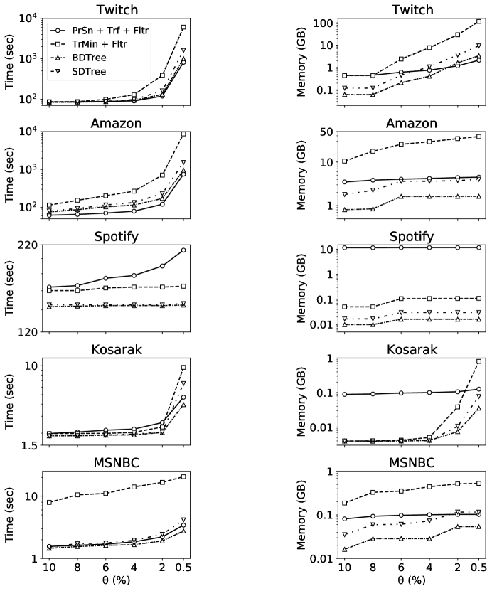
Figure 6: Total computational time and peak memory usage of BDTries, SDTries, the TreeMiner algorithm enhanced by support-based filtering (TrMin + Fltr), and the PrefixSpan algorithm enhanced by event transformation and support-based filtering (PrSn + Trf + Fltr).

Figure 6 gives the results of our comparison. In all datasets and test instances, BDTries are the most memory efficient dataset model, generally outperforming PrSn + Trf + Fltr and TreeMiner + Fltr by orders of magnitude. For example, BDTries are orders of magnitude more memory efficient than a flattened and filtered tabular-based model in the Twitch, Spotify, Kosarak, and MSNBC datasets. Trie-based models including BDTries, SDTries, and TreeMiner perform best at higher support values, benefiting more from support-based filtering. On the other hand, the memory usage of PrSn + Trf + Fltr remains relatively constant for different values of $\theta\times N$, as most of its peak memory usage is due to storing the tabular-based dataset. The memory usage of TreeMiner increases at a higher rate than SDTries or BDTries when increasing $|\mathbb{E}|$, mainly due to the increase in size of the rich information kept at each node of its trie-based model.

BDTries are not always more memory efficient than a flattened and filtered tabular-based dataset model. For example, all trie-based methods use more memory in the Twitch dataset with low minimum thresholds $\theta<2\%$. In such cases, less compression $1-|\mathcal{N}|/\sum_{\mathcal{S}_{i}\in\mathcal{SD}}|\mathcal{S}_{i}|$ is provided by trie-based models as $|\mathbb{E}|$ and $M$ are high and $N<|\mathbb{E}|^{M}$. When compression is low, for example, less than 40% as shown for the Twitch dataset in Figure 7, the memory overhead of modeling events by trie nodes is not compensated by the lower number of trie nodes. This leads to higher memory usage by trie-based models compared to tabular-based models. On the other hand, when compression is high, as shown in the remaining instances in Figure 7, trie-based methods can be considerably more memory-efficient for SPM.

In terms of total computational time, results show that PrSn + Trf + Fltr, SDTries, and BDTries are relatively competitive in all instances with the difference being a matter of seconds. Mining BDTries is slightly faster than SDTries, and in all instances faster than TreeMiner by as much as an order of magnitude on the Twitch, Amazon, and MSNBC datasets. PrSn + Trf + Fltr is the fastest approach on the Amazon dataset. This is because tabular-based models use contiguous blocks of memory to store sequences $\mathcal{S}\in\mathcal{SD}$, which is fast for lookup operations but expensive in memory usage.

We conclude that on our considered datasets, BDTries are more efficient in memory usage than SDTries, TreeMiner, and tabular-based models such as PrefixSpan, and are competitive with tabular-based models and superior to TreeMiner in terms of computational time.

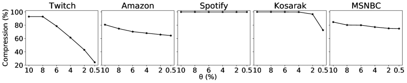
Figure 7: Total compression $\left(1-|\mathcal{N}|/\sum_{\mathcal{S}_{i}\in\mathcal{SD}}|\mathcal{S}_{i}|\right)$ provided by trie-based models, compared to tabular-based models.

5 Conclusion

In this paper, we studied memory efficient techniques for large-scale SPM. We discussed flattening and filtering techniques along with trie-based models of the dataset that can be used to lower the peak memory usage of SPM algorithms. We showed how these techniques can be used to improve both the time and memory efficiency of SPM algorithms used in the literature, with as high as an order of magnitude more memory efficiency on test instances. We developed novel SDTrie and BDTrie models of the dataset and associated mining algorithms and proved upper bounds on their memory requirements. We showed that BDTries can be orders of magnitude more memory efficient in practice compared to state-of-the-art tabular-based and trie-based mining algorithms of the literature, while remaining competitive or superior in computational time.

References

- Agrawal et al. (1994) Agrawal, R., Srikant, R., et al. Fast algorithms for mining association rules. In Proc. 20th int. conf. very large data bases, VLDB, volume 1215, pages 487–499, 1994.
- Antunes and Oliveira (2004) Antunes, C. and Oliveira, A. Sequential pattern mining algorithms: trade-offs between speed and memory, 2004.
- Bodon and Rónyai (2003) Bodon, F. and Rónyai, L. Trie: an alternative data structure for data mining algorithms. Mathematical and Computer Modelling, 38(7-9):739–751, 2003.
- Borah and Nath (2018) Borah, A. and Nath, B. Fp-tree and its variants: Towards solving the pattern mining challenges. In Proceedings of First International Conference on Smart System, Innovations and Computing, pages 535–543. Springer, 2018.
- Brost et al. (2019) Brost, B., Mehrotra, R., and Jehan, T. The music streaming sessions dataset. In The World Wide Web Conference, pages 2594–2600, 2019.
- Chen et al. (2013) Chen, C.-C., Tseng, C.-Y., and Chen, M.-S. Highly scalable sequential pattern mining based on mapreduce model on the cloud. In 2013 IEEE International Congress on Big Data, pages 310–317. IEEE, 2013.
- Chen et al. (2017) Chen, C.-C., Shuai, H.-H., and Chen, M.-S. Distributed and scalable sequential pattern mining through stream processing. Knowledge and Information Systems, 53(2):365–390, 2017.
- Chen (2009) Chen, J. An updown directed acyclic graph approach for sequential pattern mining. IEEE transactions on knowledge and data engineering, 22(7):913–928, 2009.
- El-Sayed et al. (2004) El-Sayed, M., Ruiz, C., and Rundensteiner, E. A. Fs-miner: efficient and incremental mining of frequent sequence patterns in web logs. In Proceedings of the 6th annual ACM international workshop on web information and data management, pages 128–135, 2004.
- Fournier-Viger et al. (2014) Fournier-Viger, P., Gomariz, A., Campos, M., and Thomas, R. Fast vertical mining of sequential patterns using co-occurrence information. In Pacific-Asia Conference on Knowledge Discovery and Data Mining, pages 40–52. Springer, 2014.
- Fournier-Viger et al. (2016) Fournier-Viger, P., Lin, J. C.-W., Gomariz, A., Gueniche, T., Soltani, A., Deng, Z., and Lam, H. T. The spmf open-source data mining library version 2. In Joint European conference on machine learning and knowledge discovery in databases, pages 36–40. Springer, 2016.
- Fournier-Viger et al. (2017) Fournier-Viger, P., Lin, J. C.-W., Kiran, R. U., Koh, Y. S., and Thomas, R. A survey of sequential pattern mining. Data Science and Pattern Recognition, 1(1):54–77, 2017.
- Fumarola et al. (2016) Fumarola, F., Lanotte, P. F., Ceci, M., and Malerba, D. Clofast: closed sequential pattern mining using sparse and vertical id-lists. Knowledge and Information Systems, 48(2):429–463, 2016.
- Gan et al. (2019) Gan, W., Lin, J. C.-W., Fournier-Viger, P., Chao, H.-C., and Yu, P. S. A survey of parallel sequential pattern mining. ACM Transactions on Knowledge Discovery from Data (TKDD), 13(3):1–34, 2019.
- Han et al. (2000) Han, J., Pei, J., Mortazavi-Asl, B., Chen, Q., Dayal, U., and Hsu, M. C. Freespan: frequent pattern-projected sequential pattern mining. In Proceedings of the Sixth ACM SIGKDD International Conference on Knowledge Discovery and Data Mining (KDD-2001), pages 355–359, 2000.
- Han et al. (2001) Han, J., Pei, J., Mortazavi-Asl, B., Pinto, H., Chen, Q., Dayal, U., and Hsu, M. Prefixspan: Mining sequential patterns efficiently by prefix-projected pattern growth. In proceedings of the 17th international conference on data engineering, pages 215–224, 2001.
- Han et al. (2004) Han, J., Pei, J., Yin, Y., and Mao, R. Mining frequent patterns without candidate generation: A frequent-pattern tree approach. Data mining and knowledge discovery, 8(1):53–87, 2004.
- Hosseininasab et al. (2019) Hosseininasab, A., van Hoeve, W.-J., and Cire, A. A. Constraint-based sequential pattern mining with decision diagrams. In Proceedings of the AAAI Conference on Artificial Intelligence, volume 33, pages 1495–1502, 2019.
- Huang et al. (2006) Huang, J.-W., Tseng, C.-Y., Ou, J.-C., and Chen, M.-S. On progressive sequential pattern mining. In Proceedings of the 15th ACM international conference on Information and knowledge management, pages 850–851, 2006.
- Huang et al. (2008) Huang, J.-W., Tseng, C.-Y., Ou, J.-C., and Chen, M.-S. A general model for sequential pattern mining with a progressive database. IEEE Transactions on Knowledge and Data Engineering, 20(9):1153–1167, 2008.
- Huynh et al. (2018) Huynh, B., Trinh, C., Huynh, H., Van, T.-T., Vo, B., and Snasel, V. An efficient approach for mining sequential patterns using multiple threads on very large databases. Engineering Applications of Artificial Intelligence, 74:242–251, 2018.
- Ivancsy and Vajk (2005) Ivancsy, R. and Vajk, I. Efficient sequential pattern mining algorithms. WSEAS Transactions on Computers, 4(2):96–101, 2005.
- Liao and Chen (2014) Liao, V. C.-C. and Chen, M.-S. Dfsp: a depth-first spelling algorithm for sequential pattern mining of biological sequences. Knowledge and information systems, 38(3):623–639, 2014.
- Lu and Ezeife (2003) Lu, Y. and Ezeife, C. I. Position coded pre-order linked wap-tree for web log sequential pattern mining. In Pacific-asia conference on knowledge discovery and data mining, pages 337–349. Springer, 2003.
- Mabroukeh and Ezeife (2010) Mabroukeh, N. R. and Ezeife, C. I. A taxonomy of sequential pattern mining algorithms. ACM Computing Surveys (CSUR), 43(1):1–41, 2010.
- Masseglia et al. (2000) Masseglia, F., Poncelet, P., and Cicchetti, R. An efficient algorithm for web usage mining. Networking and Information Systems Journal, 2(5/6):571–604, 2000.
- Masseglia et al. (2009) Masseglia, F., Poncelet, P., and Teisseire, M. Efficient mining of sequential patterns with time constraints: Reducing the combinations. Expert Systems with Applications, 36(2):2677–2690, 2009.
- Ni et al. (2019) Ni, J., Li, J., and McAuley, J. Justifying recommendations using distantly-labeled reviews and fine-grained aspects. In Proceedings of the 2019 Conference on Empirical Methods in Natural Language Processing and the 9th International Joint Conference on Natural Language Processing (EMNLP-IJCNLP), pages 188–197, 2019.
- Papadimitriou and Steiglitz (1998) Papadimitriou, C. H. and Steiglitz, K. Combinatorial optimization: algorithms and complexity. Courier Corporation, 1998.
- Pei et al. (2000) Pei, J., Han, J., Mortazavi-Asl, B., and Zhu, H. Mining access patterns efficiently from web logs. In Pacific-Asia Conference on Knowledge Discovery and Data Mining, pages 396–407. Springer, 2000.
- Pyun et al. (2014) Pyun, G., Yun, U., and Ryu, K. H. Efficient frequent pattern mining based on linear prefix tree. Knowledge-Based Systems, 55:125–139, 2014.
- Rappaz et al. (2021) Rappaz, J., McAuley, J., and Aberer, K. Recommendation on live-streaming platforms: Dynamic availability and repeat consumption. In Fifteenth ACM Conference on Recommender Systems, pages 390–399, 2021.
- Rizvee et al. (2020) Rizvee, R. A., Arefin, M. F., and Ahmed, C. F. Tree-miner: mining sequential patterns from sp-tree. Advances in Knowledge Discovery and Data Mining, 12085:44, 2020.
- Saleti and Subramanyam (2019) Saleti, S. and Subramanyam, R. A novel mapreduce algorithm for distributed mining of sequential patterns using co-occurrence information. Applied Intelligence, 49(1):150–171, 2019.
- Teorey (1999) Teorey, T. J. Database modeling and design. Morgan Kaufmann, 1999.
- Wang et al. (2006) Wang, J., Asanuma, Y., Kodama, E., and Takata, T. A scalable sequential pattern mining algorithm. In IEEE International Conference on Computer Systems and Applications, 2006., pages 437–444. IEEE Computer Society, 2006.
- Yang et al. (2007) Yang, S., Guo, J., and Zhu, Y. An efficient algorithm for web access pattern mining. In Fourth International Conference on Fuzzy Systems and Knowledge Discovery (FSKD 2007), volume 2, pages 726–729. IEEE, 2007.
- Yu et al. (2019) Yu, X., Li, Q., and Liu, J. Scalable and parallel sequential pattern mining using spark. World Wide Web, 22(1):295–324, 2019.