On the Convergence of SARSA with Linear Function Approximation

Abstract

SARSA, a classical on-policy control algorithm for reinforcement learning, is known to chatter when combined with linear function approximation: SARSA does not diverge but oscillates in a bounded region. However, little is known about how fast SARSA converges to that region and how large the region is. In this paper, we make progress towards this open problem by showing the convergence rate of projected SARSA to a bounded region. Importantly, the region is much smaller than the region that we project into, provided that the magnitude of the reward is not too large. Existing works regarding the convergence of linear SARSA to a fixed point all require the Lipschitz constant of SARSA’s policy improvement operator to be sufficiently small; our analysis instead applies to arbitrary Lipschitz constants and thus characterizes the behavior of linear SARSA for a new regime.

*

1 Introduction

SARSA is a classical on-policy control algorithm for reinforcement learning (RL, Sutton & Barto (2018)) dating back to Rummery & Niranjan (1994). The key idea of SARSA is to update the estimate for action values with data generated by following an exploratory and greedy policy (e.g., an $\epsilon$-greedy policy) derived from the estimate itself. In this paper, we refer to the operator used for deriving such a policy from the action value estimate as the policy improvement operator.

The study of SARSA begins in the tabular setting, where the action value estimates are stored in the form of a look-up table. For example, Singh et al. (2000) confirm the asymptotic convergence of SARSA to the optimal policy provided that the policies from the policy improvement operator satisfy the “greedy in the limit with infinite exploration” condition. Tabular methods, however, are not preferred when the state space is large and generalization is required across states. One possible solution is linear function approximation, which approximates the action values via the inner product of state-action features and a learnable weight vector. The behavior of SARSA with linear function approximation (linear SARSA) is, however, less understood.

	Gordon	Perkins & Precup	Melo et al.	Zou et al.	Ours
convergence	to a region	to a point	to a point	to a point	to a region
per-step policy improvement	✗	✗	✓	✓	✓
any Lipschitz constant	✓	✓∗	✗	✗	✓
convergence rate	✗	✗	✗	✓	✓

Table 1: Comparison with existing works. ✓^∗ indicates that the corresponding property is not explicitly documented in the original work. “Per-step policy improvement” means that the policy improvement operator is applied every time step.

Gordon (1996) and Bertsekas & Tsitsiklis (1996) empirically observe that linear SARSA can chatter: the weight vector does not go to infinity (i.e., it does not diverge) but oscillates in a bounded region. Importantly, this chattering behavior remains even if a decaying learning rate is used. Gordon (2001) further proves that trajectory-based linear SARSA with an $\epsilon$-greedy policy improvement operator converges to a bounded region asymptotically. Unlike standard linear SARSA, where the policy improvement operator is invoked every step to generate a new policy for action selection in the next step, trajectory-based linear SARSA generates a policy at the beginning of each episode and the policy remains fixed during the episode. Intuitively, within an episode, trajectory-based linear SARSA is just linear Temporal Difference (TD, Sutton (1988)) learning for evaluating action values. It, therefore, converges to an approximation of the action value function of the policy generated at the beginning of the episode (Tsitsiklis & Roy, 1996). Since the number of all possible $\epsilon$-greedy policies is finite in a finite Markov Decision Process with a fixed $\epsilon$, trajectory-based linear SARSA oscillates among the (approximate) action value functions of those $\epsilon$-greedy policies, which form a bounded region. Later, Perkins & Precup (2002) prove the asymptotic convergence of fitted linear SARSA (a.k.a. model-free approximate policy iteration) to a fixed point. Similar to trajectory-based SARSA, fitted SARSA alternates between thorough TD learning for policy evaluation under a fixed policy and the application of the policy improvement operator. In other words, it involves bi-level optimization. Then assuming the Lipschitz constant of the policy improvement operator is sufficiently small such that the composition of the policy improvement operator and some other function becomes contractive, convergence of fitted SARSA is obtained thanks to Banach’s fixed point theorem. Despite this progress, the asymptotic behavior of standard linear SARSA, which invokes the policy improvement operator every time step, still remains unclear, as does a potential convergence rate. Understanding the behavior of linear SARSA is one of the four open theoretical questions in RL raised by Sutton (1999).

Several efforts have been made to analyze linear SARSA. Melo et al. (2008) prove the asymptotic convergence of linear SARSA. Zou et al. (2019) further provide a convergence rate of a projected linear SARSA, which uses an additional projection operator in the canonical linear SARSA update. Unlike Gordon (2001), the convergence in Melo et al. (2008); Zou et al. (2019) is to a fixed point instead of a bounded region. Although convergence to a fixed point is preferred, Melo et al. (2008); Zou et al. (2019) require that SARSA’s policy improvement operator is Lipschitz continuous and the Lipschitz constant is sufficiently small. It remains an open problem how linear SARSA behaves when the Lipschitz constant is large.

This problem is of interest because to our knowledge, most meaningful empirical results using SARSA for control consider an $\epsilon$-greedy policy or a softmax policy. The former behaves similarly to a Lipschitz continuous policy improvement operator with a very large Lipschitz constant. The latter is usually tuned such that its Lipschitz constant is reasonably large. We refer the reader to Section 2 for more discussion about those two classes of policy improvement operators and now name a few notable empirical results. In the tabular setting, Sutton & Barto (2018) use an $\epsilon$-greedy policy with $\epsilon=0.1$ in the Windy GridWorld. With linear function approximation, Rummery & Niranjan (1994) use a softmax policy in a robot control problem with the temperature decaying from $0.05$ to $0.01$ such that the softmax policy has a reasonably large Lipschitz constant. Liang et al. (2015) use an $\epsilon$-greedy policy with $\epsilon=0.01$ to play all Atari games (Bellemare et al., 2013). In deep RL, Mnih et al. (2016) use $\epsilon$-greedy policies with decaying $\epsilon$ in their asynchronous methods for playing Atari games. Besides the aforementioned interest from the empirical side, this problem has also been recognized as an important theoretical open problem in Perkins & Precup (2002); Zou et al. (2019).

In this paper, we make contributions to this open problem. In particular, we study the projected linear SARSA (Zou et al., 2019) and show that it converges to a bounded region regardless of the magnitude of the Lipschitz constant of the policy improvement operator. Importantly, the bounded region is much smaller than the region we project into provided that the magnitude of rewards is not too large. The differences between our work and existing works are summarized in Table 1.

2 Background

In this paper, all vectors are column. We use ${\left<x,y\right>}\doteq x^{\top}y$ to denote the standard inner product in Euclidean spaces. For a positive definite matrix $D$, we use $\norm{x}_{D}\doteq\sqrt{x^{\top}Dx}$ to denote the vector norm induced by $D$. We overload $\norm{\cdot}_{D}$ to also denote the induced matrix norm. We write $\norm{\cdot}$ as shorthand for $\norm{\cdot}_{I}$, where $I$ is the identity matrix, i.e., $\norm{\cdot}$ denotes the standard $\ell_{2}$ norm. When it does not cause confusion, we use vectors and functions interchangeably. For example, if $f$ is a function $\mathcal{S}\to\mathbb{R}$, we also use $f$ to denote the vector in $\mathbb{R}^{{|\mathcal{S}|}}$ whose $s$-indexed element is $f(s)$.

We consider an infinite horizon Markov Decision Process (MDP, Puterman (2014)) with a finite state space $\mathcal{S}$, a finite action space $\mathcal{A}$, a transition kernel $p:\mathcal{S}\times\mathcal{S}\times\mathcal{A}\to[0,1]$, a reward function $r:\mathcal{S}\times\mathcal{A}\to[-r_{max},r_{max}]$, a discount factor $\gamma$, and an initial distribution $p_{0}:\mathcal{S}\to[0,1]$. At time step $t=0$, an initial state $S_{0}$ is sampled from $p_{0}(\cdot)$. At time step $t$, an agent at a state $S_{t}$ takes an action $A_{t}\sim\pi(\cdot|S_{t})$ according to a policy $\pi:\mathcal{A}\times\mathcal{S}\to[0,1]$. The agent then receives a reward $R_{t+1}\doteq r(S_{t},A_{t})$ and proceeds to a successor state $S_{t+1}\sim p(\cdot|S_{t},A_{t})$. The return at time step $t$ is defined as $G_{t}\doteq\sum_{i=0}^{\infty}\gamma^{i}R_{t+i+1}$, which allows us to define the action value function as

$$\textstyle q_{\pi}(s,a)\doteq\mathbb{E}\left[G_{t}|S_{t}=s,A_{t}=a,\pi,p\right].$$ (1)

The action value function $q_{\pi}$ is closely related to the Bellman operator $\mathcal{T}_{\pi}$, which is defined as $\mathcal{T}_{\pi}q\doteq r+\gamma P_{\pi}q$, where $P_{\pi}\in\mathbb{R}^{{|\mathcal{S}\times\mathcal{A}|}\times{|\mathcal{S}\times\mathcal{A}|}}$ is the state-action pair transition matrix, i.e., $P_{\pi}\left((s,a),(s^{\prime},a^{\prime})\right)\doteq p(a^{\prime}|s,a)\pi(a^{\prime}|s^{\prime})$. In particular, $q_{\pi}$ is the only vector $q\in\mathbb{R}^{|\mathcal{S}\times\mathcal{A}|}$ satisfying $q=\mathcal{T}_{\pi}q$. The goal of control is to find an optimal policy $\pi_{*}$ such that $\forall\pi,s,a$, $q_{\pi_{*}}(s,a)\geq q_{\pi}(s,a)$. All optimal policies share the same action value function, which is referred to as $q_{*}$. One classical approach for finding $q_{*}$ is SARSA, which updates an estimate $q\in\mathbb{R}^{|\mathcal{S}\times\mathcal{A}|}$ iteratively as

$$A_{t+1} \sim\pi_{q}(\cdot|S_{t+1}),$$ (2)

$$\delta_{t} \leftarrow R_{t+1}+\gamma q(S_{t+1},A_{t+1})-q(S_{t},A_{t})$$ (3)

$$q(S_{t},A_{t}) \leftarrow q(S_{t},A_{t})+\alpha_{t}\delta_{t},$$ (4)

where $\quantity{\alpha_{t}}$ is a sequence of learning rates and $\pi_{q}$ denotes that the policy $\pi$ is parameterized by the action value estimate $q$. A commonly used $\pi_{q}$ is an $\epsilon$-greedy policy, i.e.,

$$\pi_{q}(a|s)=\begin{cases}\frac{\epsilon}{\absolutevalue{\mathcal{A}}},\quad a\neq\arg\max_{b\in\mathcal{A}}q(s,b)\\ 1-\epsilon+\frac{\epsilon}{\absolutevalue{\mathcal{A}}},\mbox{\quad otherwise\quad}\end{cases},$$ (5)

where $\epsilon\in[0,1]$ is a hyperparameter. Another common example is an $\epsilon$-softmax policy, i.e.,

$$\textstyle\pi_{q}(a|s)=\frac{\epsilon}{{|\mathcal{A}|}}+(1-\epsilon)\frac{\exp(q(s,a)/\iota)}{\sum_{b}\exp(q(s,b)/\iota)},$$ (6)

where $\iota\in(0,\infty)$ is the temperature of the softmax function. This $\pi_{q}$ is exactly the policy improvement operator discussed in Section 1: it maps an action value estimate $q$ to a new policy; it is “improvement” in that it usually has greedification over the action value estimate to some extent. The $\epsilon$-softmax policy $\pi_{q}$ in (6) is Lipschitz continuous in $q$ with the Lipschitz constant being $\frac{1-\epsilon}{\iota}$. When the temperature $\iota$ approaches $0$, the $\epsilon$-softmax policy approaches the $\epsilon$-greedy policy. Therefore, despite the $\epsilon$-greedy policy is not even continuous, it is the limit of a sequence of Lipschitz continuous policies with the Lipschitz constants approaching infinity. We, therefore, argue that an $\epsilon$-greedy policy would empiricially behave similarly to a Lipschitz continuous policy with a very large Lipschitz constant.

So far we have considered only time-homogeneous policies. One can also consider time-inhomogeneous policies, e.g., a policy $\pi_{q,t}(a|s)$ that depends on both the action value estimate $q$ and the time step $t$. Singh et al. (2000) show that if the time-inhomogeneous policies $\pi_{q,t}$ satisfy the “greedy in the limit with infinite exploration” (GLIE) condition then the iterates generated by (2) converge to $q_{*}$ almost surely.

It is, however, not always practical to use a look-up table for storing our action value estimates, especially when the state space is large or generalization is required across states. One natural solution is linear function approximation, where the action value estimate $q(s,a)$ is parameterized as $x(s,a)^{\top}w$. Here $x:\mathcal{S}\times\mathcal{A}\to\mathbb{R}^{K}$ is the feature function which maps a state-action pair to a $K$-dimensional vector and $w\in\mathbb{R}^{K}$ is the learnable weight vector. We use $X\in\mathbb{R}^{{|\mathcal{S}\times\mathcal{A}|}\times K}$ to denote the feature matrix, whose $(s,a)$-indexed row is $x(s,a)^{\top}$. We use as shorthand

$$\textstyle\pi_{w}\doteq\pi_{Xw},\,x_{t}\doteq x(S_{t},A_{t}),\,x_{max}\doteq\max_{s,a}\norm{x(s,a)}.$$ (7)

  Initialize $w_{0}$ such that $\norm{w_{0}}\leq C_{\Gamma}$

  $S_{0}\sim p_{0}(\cdot),A_{0}\sim\pi_{w_{0}}(\cdot|S_{0})$

  $t\leftarrow 0$

  while true do

     Execute $A_{t}$, get $R_{t+1},S_{t+1}$  

     Sample $A_{t+1}\sim\pi_{w_{t}}(\cdot|S_{t+1})$  

     $\delta_{t}\leftarrow R_{t+1}+\gamma x_{t+1}^{\top}w_{t}-x_{t}^{\top}w_{t}$  

     $w_{t+1}\leftarrow\Gamma\left(w_{t}+\alpha_{t}\delta_{t}x_{t}\right)$  

     $t\leftarrow t+1$  

  end while

Algorithm 1 SARSA with linear function approximation

SARSA (Algorithm 1) is a commonly used algorithm for learning $w$. In Algorithm 1, $\Gamma:\mathbb{R}^{K}\to\mathbb{R}^{K}$ is a projection operator onto a ball of radius $C_{\Gamma}$, i.e.,

$$\textstyle\Gamma(w)\doteq\begin{cases}w,&\norm{w}\leq C_{\Gamma},\\ C_{\Gamma}\frac{w}{\norm{w}},&\norm{w}>C_{\Gamma}\end{cases}.$$ (8)

For now we consider the setting where $C_{\Gamma}=\infty$, i.e., $\Gamma$ is an identity mapping. If the iterates $\quantity{w_{t}}$ generated by SARSA converged to some vector $w_{*}$, the expected update at $w_{*}$ would have to diminish, i.e.,

$$\mathbb{E}_{S_{t},A_{t}\sim d_{\pi_{w_{*}}}}\left[\left(R_{t+1}+\gamma x_{t+1}^{\top}w_{*}-x_{t}^{\top}w_{*}\right)x_{t}\right]=0,$$ (9)

where for a policy $\pi$, we use $d_{\pi}\in\mathbb{R}^{|\mathcal{S}\times\mathcal{A}|}$ to denote the stationary state action pair distribution of the chain in $\mathcal{S}\times\mathcal{A}$ induced by $\pi$ (assuming it exists). We can equivalently write (9) in a matrix form as

$$X^{\top}D_{\pi_{w_{*}}}(r+\gamma P_{\pi_{w_{*}}}Xw_{*}-Xw_{*})=0,$$ (10)

where for a policy $\pi$, we use $D_{\pi}\in\mathbb{R}^{{|\mathcal{S}\times\mathcal{A}|}\times{|\mathcal{S}\times\mathcal{A}|}}$ to denote a diagonal matrix whose diagonal entry is $d_{\pi}$. By defining

$$A_{\pi}\doteq X^{\top}D_{\pi}(\gamma P_{\pi}-I)X,\,b_{\pi}\doteq X^{\top}D_{\pi}r,$$ (11)

(10) becomes $A_{\pi_{w_{*}}}w_{*}+b_{\pi_{w_{*}}}=0$. It is known (see, e.g., Tsitsiklis & Roy (1996)) that $A_{\pi}$ is negative definite under mild conditions. We define a projection operator $\Pi_{D_{\pi}}$ mapping a vector in $\mathbb{R}^{|\mathcal{S}\times\mathcal{A}|}$ to the column space of $X$ as

$$\textstyle\Pi_{D_{\pi}}q\doteq\arg\min_{\hat{q}\in col(X)}\norm{\hat{q}-q}_{D_{\pi}}^{2},$$ (12)

where $col(X)$ denotes the column space of $X$. It can be computed that $\Pi_{D_{\pi}}=X\left(X^{\top}D_{\pi}X\right)^{-1}X^{\top}D_{\pi}$ and it is known (see, e.g., De Farias & Van Roy (2000)) that (10) holds if and only if $\Pi_{D_{\pi_{w_{*}}}}\mathcal{T}_{\pi_{w_{*}}}Xw_{*}=Xw_{*}$. In other words, $Xw_{*}$ is a fixed point of the operator $\mathcal{H}(q)\doteq\Pi_{D_{\pi_{q}}}\mathcal{T}_{\pi_{q}}q$. The operator $\mathcal{H}$ is referred to as the approximate policy iteration operator and SARSA is an incremental, stochastic method to find a fixed point of approximate policy iteration. Unfortunately, when $\pi_{q}(a|s)$ is not continuous in $q$ (e.g., $\pi_{q}$ is an $\epsilon$-greedy policy, c.f. (5)), $\mathcal{H}$ does not necessarily have a fixed point (De Farias & Van Roy, 2000). Conversely, when $\pi_{q}(a|s)$ is continuous in $q$, De Farias & Van Roy (2000) show that $\mathcal{H}$ has at least one fixed point.

Perkins & Precup (2002) assume $\pi_{q}$ is Lipschitz continuous in $q$ and study a form of fitted SARSA, which is a model-free variant of approximate policy iteration. At the $k$-th iteration, Perkins & Precup (2002) first invoke TD for learning the action value function of $\pi_{k}$, which converges to $w_{k}=A^{-1}_{\pi_{k}}b_{\pi_{k}}$ after infinitely many steps. Then the policy for the $(k+1)$-th iteration is obtained via invoking the policy improvement operator, i.e., $\pi_{k+1}\doteq\pi_{w_{k}}$. Perkins & Precup (2002) show that

$$\textstyle\norm{\pi_{A_{\hat{\pi}}^{-1}b_{\hat{\pi}}}-\pi_{A_{\pi^{\prime}}^{-1}b_{\pi^{\prime}}}}\leq\mathcal{O}\left(L_{\pi}\right)\norm{\hat{\pi}-\pi^{\prime}},$$ (13)

where the policies $\hat{\pi}$ and $\pi^{\prime}$ should be interpreted as vectors in $\mathbb{R}^{{|\mathcal{S}\times\mathcal{A}|}}$ whose $(s,a)$-indexed element is $\pi(a|s)$ when computing $\norm{\hat{\pi}-\pi^{\prime}}$ and $L_{\pi}$ denotes the Lipschitz constant of the policy improvement operator $\pi_{w}$, i.e., $\forall s,a$,

$$\absolutevalue{\pi_{w_{1}}(a|s)-\pi_{w_{2}}(a|s)}\leq L_{\pi}\norm{w_{1}-w_{2}}.$$ (14)

Consequently, if $L_{\pi}$ is sufficiently small, the function $x\to\pi_{A^{-1}_{x}b_{x}}$, which maps $\pi_{k}$ to $\pi_{k+1}$, becomes a contraction. Banach’s fixed point theorem then confirms the convergence of fitted SARSA. From the definition of $A_{\pi}$ and $b_{\pi}$ in (11), it is easy to see that (13) can also be expressed as

$$\norm{\pi_{A_{\hat{\pi}}^{-1}b_{\hat{\pi}}}-\pi_{A_{\pi^{\prime}}^{-1}b_{\pi^{\prime}}}}\leq\mathcal{O}\left(L_{\pi}\norm{r}\right)\norm{\hat{\pi}-\pi^{\prime}}$$ (15)

because $r$ is a multiplier in the definition of $b_{\pi}$. Hence, for any $L_{\pi}$, if the magnitude of the reward $\norm{r}$ is small enough, the function $x\to\pi_{A^{-1}_{x}b_{x}}$ is contractive and fitted SARSA remains convergent. Nevertheless, Perkins & Precup (2002) share the same spirit as Gordon (2001) by holding the policy fixed for sufficiently (possibly infinitely) many steps to wait for the policy evaluation to complete.

When it comes to standard linear SARSA that updates the policy every time step, Melo et al. (2008) consider, for a fixed point $w_{*}$,

$$\textstyle C_{w_{*}}\doteq\sup_{w}\norm{A_{\pi_{w}}-A_{\pi_{w_{*}}}}+\sup_{w\neq w_{*}}\frac{\norm{b_{\pi_{w}}-b_{\pi_{w_{*}}}}}{\norm{w-w_{*}}}.$$ (16)

They show that $C_{w_{*}}=\mathcal{O}\left(L_{\pi}\right)$ and if $L_{\pi}$ is small enough such that

$$A_{\pi_{w_{*}}}+C_{w_{*}}I$$ (17)

is negative definite, SARSA converge to $w_{*}$. The convergence of SARSA in Perkins & Precup (2002); Melo et al. (2008) does not require the projection operator (i.e., $C_{\Gamma}=\infty$) but is only asymptotic, Zou et al. (2019) further provide a convergence rate of SARSA using some $C_{\Gamma}<\infty$, assuming $L_{\pi}$ is small enough such that

$$A_{\pi_{w_{*}}}+\mathcal{O}\left(L_{\pi}\left(r_{max}+2x_{max}C_{\Gamma}\right)\right)I$$ (18)

is negative definite. It is easy to see that if $L_{\pi}$ is not small enough, neither (17) nor (18) can be guaranteed to be negative definite no matter how small $\norm{r}$ is. This is because the $\sup_{w}\norm{A_{\pi_{w}}-A_{\pi_{w_{*}}}}$ term in $C_{w_{*}}$ and the $2x_{max}C_{\Gamma}$ term in (18) are independent of $r$. In other words, unlike Perkins & Precup (2002), where the requirement for a sufficiently small $L_{\pi}$ is not necessary when the magnitude of the reward is enough, a sufficiently small $L_{\pi}$ is an essential requirement for the analysis of Melo et al. (2008); Zou et al. (2019). We, however, note that requring a finite $C_{\Gamma}$ and a sufficiently small $L_{\pi}$ can be restrictive. To see this, consider the $\epsilon$-softmax policy in (6). On the one hand, for this parameterization, we have $L_{\pi}=\frac{1-\epsilon}{\iota}$. For $L_{\pi}$ to be sufficiently small, we have to ensure the temperature $\iota$ to be sufficiently large. On the other hand, a finte $C_{\Gamma}$ ensures that the action value estimate $q(s,a)$ inside $\exp(\cdot)$ is bounded. Combining the two facts together, it is easy to see that the $\epsilon$-softmax policy cannot be much different from a uniformly random policy. Or more formally speaking, the probability of any action is at most

$$\frac{\epsilon}{{|\mathcal{A}|}}+\frac{1-\epsilon}{1+\left({|\mathcal{A}|}-1\right)\exp\left(-\frac{2x_{max}C_{\Gamma}}{\iota}\right)}.$$ (19)

When $\iota$ is too large, the above probability approaches $\frac{1}{{|\mathcal{A}|}}$, making it hard to ensure sufficient exploitation. The behavior of SARSA with a large $L_{\pi}$, however, remains an open problem.

3 Stochastic Approximation with Rapidly Changing Markov Chains

To prepare us for the analysis of SARSA, we show, in this section, a convergence rate (to a bounded region) of a generic stochastic approximation algorithm. More precisely, we consider the following iterative updates:

$$w_{t+1}\doteq\Gamma\left(w_{t}+\alpha_{t}\left(F_{\theta_{t}}(w_{t},Y_{t})-w_{t}\right)\right).$$ (20)

Here $\quantity{w_{t}\in\mathbb{R}^{K}}$ are the iterates generated by the stochastic approximation algorithm, $\quantity{Y_{t}}$ is a sequence of random variables evolving in a finite space $\mathcal{Y}$, $\quantity{\theta_{t}\in\mathbb{R}^{L}}$ is a sequence of random variables controlling the transition of $\quantity{Y_{t}}$, $F_{\theta}$ is a function from $\mathbb{R}^{K}\times\mathcal{Y}$ to $\mathbb{R}^{K}$ parameterized by $\theta$, and $\Gamma$ is the projection operator defined in (8). Importantly, we consider the setting where

$$\forall t,\theta_{t}\equiv w_{t}.$$ (21)

In other words, there is only a single iterate in our setting. To ease presentation, we use $\quantity{w_{t}}$ and $\quantity{\theta_{t}}$ to denote the same quantity. This emphasizes their different roles as the iterates of interest and as the controller of the transition kernel.

Our analysis is a natural extension of Chen et al. (2021) and Zhang et al. (2022) but has significant differences to theirs. Chen et al. (2021) consider a time-homogeneous Markov chain (i.e., $\forall t,\theta_{t}\equiv\theta_{0}$). Consequently, their results are naturally applicable to policy evaluation problems. Zhang et al. (2022) consider a time-inhomogeneous Markov chain, where the iterates $\quantity{w_{t}}$ are different from the sequence $\quantity{\theta_{t}}$. More importantly, Zhang et al. (2022) assume that $\quantity{\theta_{t}}$ changes sufficiently slowly, i.e., there exists another sequence $\quantity{\beta_{t}}$ such that

$$\norm{\theta_{t+1}-\theta_{t}}=\mathcal{O}\left(\beta_{t}\right),\,\lim_{t\to\infty}\frac{\beta_{t}}{\alpha_{t}}=0.$$ (22)

This is the classical two-timescale setting (see, e.g., Borkar (2009)) and their analysis naturally applies to actor-critic algorithms (Konda & Tsitsiklis, 1999) with $\quantity{w_{t}}$ and $\quantity{\theta_{t}}$ interpreted as critic and actor respectively. We instead consider the setting where $\forall t,\theta_{t}=w_{t}$. In other words, the time-inhomogeneous Markov chain we consider changes rapidly, which is the main challenge of our analysis. As a consequence, we introduce the projection operator $\Gamma$, not required in Chen et al. (2021); Zhang et al. (2022). The price is that we only show convergence to a bounded region while Chen et al. (2021); Zhang et al. (2022) show convergence to points. Convergence to a bounded region is, however, sufficient for our purpose of understanding the behavior of SARSA since it matches what practitioners have observed. Furthermore, we believe our analysis might be applicable to other RL algorithms and might also have independent interest beyond RL. We now state our assumptions.

Assumption 3.1.

(Time-inhomogeneous Markov chain) There exists a family of parameterized transition matrices $\Lambda_{P}\doteq\quantity{P_{\theta}\in\mathbb{R}^{|\mathcal{Y}|\times|\mathcal{Y}|}|\theta\in\mathbb{R}^{L}}$ such that

$$\Pr(Y_{t+1}=y)=P_{\theta_{t+1}}(Y_{t},y).$$ (23)

Assumption 3.2.

(Uniform ergodicity) Let $\bar{\Lambda}_{P}$ be the closure of $\Lambda_{P}$. For any $P\in\bar{\Lambda}_{P}$, the chain induced by $P$ is ergodic. We use $d_{\theta}$ to denote the invariant distribution of the chain induced by $P_{\theta}$.

Those two assumptions are identical to those of Zhang et al. (2022). Assumption 3.1 states that the random process $\quantity{Y_{t}}$ is a time-inhomogeneous Markov chain. Assumption 3.2 states the ergodicity of the Markov chains. Assumption 3.2 is also used in the analysis of RL algorithms in both on-policy (Marbach & Tsitsiklis, 2001) and off-policy (Zhang et al., 2022, 2021) settings. We later show how SARSA($\lambda$) can trivially fulfill Assumption 3.2. The uniform ergodicity in Assumption 3.2 immediately implies uniform mixing.

Lemma 3.3.

(Lemma 1 of Zhang et al. (2022)) Let Assumption 3.2 hold. Then, there exist constants $C_{M}>0$ and $\tau\in(0,1)$, independent of $\theta$, such that for any $n>0$,

$$\textstyle\sup_{y,\theta}\sum_{y^{\prime}}\absolutevalue{P^{n}_{\theta}(y,y^{\prime})-d_{\theta}(y^{\prime})}\leq C_{M}\tau^{n}.$$ (24)

As noted in Zhang et al. (2022), the uniform mixing property in Lemma 3.3 is usually a direct technical assumption in previous works (e.g., Zou et al. (2019); Wu et al. (2020)).

Assumption 3.4.

(Uniform pseudo-contraction) Let

$$\bar{F}_{\theta}(w) \doteq\sum_{y\in\mathcal{Y}}d_{\theta}(y)F_{\theta}(w,y),$$ (25)

$$f^{\alpha}_{\theta}(w) \doteq w+\alpha\left(\bar{F}_{\theta}(w)-w\right).$$ (26)

Then,

1. For any $\theta$, $\bar{F}_{\theta}$ has a unique fixed point, i.e., there exists a unique $w^{*}_{\theta}$ such that

   $$\bar{F}_{\theta}(w^{*}_{\theta})=w^{*}_{\theta}.$$ (27)

2. There exists a constant $\bar{\alpha}>0$ such that for all $\alpha\in(0,\bar{\alpha})$, $f^{\alpha}_{\theta}$ is a uniform pseudo-contraction, i.e., there exists a constant $\kappa_{\alpha}\in(0,1)$ (depending on $\alpha$), such that for all $\theta,w$,

   $$\norm{f^{\alpha}_{\theta}(w)-w^{*}_{\theta}}\leq\kappa_{\alpha}\norm{w-w^{*}_{\theta}}.$$ (28)

Assumption 3.4 is another difference from Chen et al. (2021); Zhang et al. (2022). Namely, Chen et al. (2021); Zhang et al. (2022) require $\bar{F}_{\theta}$ to be a contraction while we only require $f_{\theta}^{\alpha}$ to be a pseudo-contraction. It is easy to see that the contraction of $\bar{F}_{\theta}$ immediately implies the pseudo-contraction of $f_{\theta}^{\alpha}$ but not in the opposite direction. In other words, our assumption is weaker.

Assumption 3.5.

(Continuity and boundedness) There exist constants $L_{F},L_{F}^{\prime},L_{F}^{\prime\prime},U_{F},U_{F}^{\prime},U_{F}^{\prime\prime},L_{w},U_{w},L_{P}$ such that for any $w,w^{\prime},y,y^{\prime},\theta,\theta^{\prime}$,

1. $\norm{F_{\theta}(w,y)-F_{\theta}(w^{\prime},y)}\leq L_{F}\norm{w-w^{\prime}}$

2. $\norm{F_{\theta}(w,y)-F_{\theta^{\prime}}(w,y)}\leq L_{F}^{\prime}\norm{\theta-\theta^{\prime}}(\norm{w}+U_{F}^{\prime})$

3. $\norm{F_{\theta}(0,y)}\leq U_{F}$

4. $\norm{\bar{F}_{\theta}(w)-\bar{F}_{\theta^{\prime}}(w)}\leq L_{F}^{\prime\prime}\norm{\theta-\theta^{\prime}}(\norm{w}+U_{F}^{\prime\prime})$

5. $\norm{w^{*}_{\theta}-w^{*}_{\theta^{\prime}}}\leq L_{w}\norm{\theta-\theta^{\prime}}$

6. $\sup_{\theta}\norm{w^{*}_{\theta}}\leq U_{w}$

7. $\absolutevalue{P_{\theta}(y,y^{\prime})-P_{\theta^{\prime}}(y,y^{\prime})}\leq L_{P}\norm{\theta-\theta^{\prime}}$

Assumption 3.5 states some regularity conditions for the functions we consider and is identical to that of Zhang et al. (2022).

Assumption 3.6.

(Projection)

1. $\norm{w_{0}}\leq C_{\Gamma},U_{w}\leq C_{\Gamma}$.

2. For any $\theta,w,y$, we have

   $$P_{\theta} =P_{\Gamma(\theta)},\,F_{\theta}(w,y)=F_{\Gamma(\theta)}(w,y),$$ (29)

   $$w^{*}_{\theta} =w^{*}_{\Gamma(\theta)}.$$ (30)

Assumption 3.6 requires that some of the functions we consider are invariant to the projection operator. We will later show that SARSA($\lambda$) trivially satisfies this assumption.

Assumption 3.7.

The learning rates $\quantity{\alpha_{t}}$ have the form

$$\textstyle\alpha_{t}\doteq\frac{c_{\alpha}}{(t_{0}+t)^{\epsilon_{\alpha}}},$$ (31)

where $c_{\alpha}>0,\epsilon_{\alpha}\in(0,1],t_{0}>0$ are constants to be tuned.

Assumption 3.7 is just one of many possible forms of learning rates; we use this particular one to ease presentation. Importantly, the learning rates $\quantity{\alpha_{t}}$ here do not verify the Robbins-Monro’s condition (Robbins & Monro, 1951) when $\epsilon_{\alpha}\leq 0.5$, neither do the learning rates in Wu et al. (2020); Chen et al. (2021).

We now present our analysis. Given the sequences $\quantity{\theta_{t}}$ (i.e., $\quantity{w_{t}}$) and $\quantity{Y_{t}}$ in (20), we define an auxiliary sequence $\quantity{u_{t}}$ as

$$u_{0}\doteq w_{0},$$ (32)

$$u_{t+1}\doteq \Gamma(u_{t})+\alpha_{t}(F_{\theta_{t}}(\Gamma(u_{t}),Y_{t})-\Gamma(u_{t})).$$ (33)

Lemma 3.8.

Let Assumption 3.6 hold. Then for any $t$, $w_{t}=\Gamma(u_{t})$.

Proof.

It follows immediately from induction. ∎

Intuitively, $\quantity{u_{t}}$ is simply the pre-projection version of $\quantity{w_{t}}$. We are interested in $\quantity{u_{t}}$ because it has the following nice property.

Theorem 3.9.

Let Assumptions 3.1 - 3.7 hold. If $t_{0}$ is sufficiently large, then the iterates $\quantity{u_{t}}$ generated by (33) satisfy

$$\mathbb{E}\left[\norm{u_{t+1}-w^{*}_{\theta_{t+1}}}^{2}\right]$$ (34)

$$\leq \left(1-2\left(1-\kappa_{\alpha_{t}}-\mathcal{O}\left(\alpha_{t}^{2}\log^{2}\alpha_{t}\right)\right)\right)\mathbb{E}\left[\norm{\Gamma(u_{t})-w^{*}_{\theta_{t}}}^{2}\right]$$ (35)

$$+2L_{w}L_{\theta}\alpha_{t}\mathbb{E}\left[\norm{\Gamma(u_{t})-w^{*}_{\theta_{t}}}\right]+\mathcal{O}\left(\alpha_{t}^{2}\log^{2}\alpha_{t}\right),$$ (36)

where $L_{\theta}\doteq U_{F}+(L_{F}+1)C_{\Gamma}$.

See Section A.1 for the proof of Theorem 3.9, where the constants hidden by $\mathcal{O}\left(\cdot\right)$ and how large $t_{0}$ is are also explicitly documented. Theorem 3.9 gives a recursive form of some error terms. We, however, cannot go further unless we have the domain knowledge of $\kappa_{\alpha}$.

Corollary 3.10.

Let Assumptions 3.1 - 3.7 hold. Assume $\kappa_{\alpha}=\sqrt{1-\eta\alpha}$ for some positive constant $\eta>0$. If $t_{0}$ is sufficiently large, then the iterates $\quantity{w_{t}}$ generated by (20) satisfy

$$\mathbb{E}\left[\norm{w_{t}-w^{*}_{w_{t}}}^{2}\right]=\frac{72L_{w}^{2}L_{\theta}^{2}}{\eta^{2}}$$ (37)

$$+ \begin{cases}\mathcal{O}\left(t^{-\frac{\eta c_{\alpha}}{3}}\log^{2}t\right),&\epsilon_{\alpha}=1,\eta c_{\alpha}\in(0,3)\\ \mathcal{O}\left(\frac{\log^{3}t}{t}\right),&\epsilon_{\alpha}=1,\eta c_{\alpha}=3\\ \mathcal{O}\left(\frac{\log^{2}t}{t}\right),&\epsilon_{\alpha}=1,\eta c_{\alpha}\in(3,\infty)\\ \mathcal{O}\left(\frac{\log^{2}t}{t^{\epsilon_{\alpha}}}\right),&\epsilon_{\alpha}\in(0,1)\end{cases}.$$ (38)

See Section A.2 for the proof of Corollary 3.10, as well as the constants hidden by $\mathcal{O}\left(\cdot\right)$ and how large $t_{0}$ is. Due to the projection operator, we have the bound

$$\textstyle\mathbb{E}\left[\norm{w_{t}-w^{*}_{w_{t}}}^{2}\right]\leq 4C_{\Gamma}^{2}.$$ (39)

So Corollary 3.10 is informative only if

$$\textstyle\frac{72L_{w}^{2}L_{\theta}^{2}}{\eta^{2}}\leq 4C_{\Gamma}^{2}.$$ (40)

This is where we need more domain knowledge and the analysis in the next section provides an example.

4 SARSA with Linear Function Approximation

We first analyze SARSA and expected SARSA with the following assumptions.

Assumption 4.1.

(Lipschitz continuity) There exists $L_{\pi}>0$ such that $\forall w,w^{\prime},a,s$,

$$\norm{\pi_{w}(a|s)-\pi_{w^{\prime}}(a|s)} \leq L_{\pi}\norm{w-w^{\prime}}.$$ (41)

Assumption 4.2.

(Uniform ergodicity) Let $\bar{\Lambda}_{\pi}$ be the closure of $\quantity{\pi_{w}\mid w\in\mathbb{R}^{|\mathcal{S}\times\mathcal{A}|}}$. For any $\pi\in\bar{\Lambda}_{\pi}$, the chain induced by $\pi$ is ergodic and $\pi(a|s)>0$.

Assumption 4.3.

(Linear independence) The feature matrix $X$ has full column rank.

Assumption 4.1 is also used in Perkins & Precup (2002); Melo et al. (2008); Zou et al. (2019). As noted by Zhang et al. (2022), Assumption 4.2 is easy to fulfill especially when the chain induced by a uniformly random policy is ergodic, which we believe is a fairly weak assumption. An example policy satisfying those two assumptions is the $\epsilon$-softmax policy in (6) with any $\epsilon\in(0,1]$, provided that the chain induced by a uniformly random policy is ergodic. Assumption 4.3 is standard in the literature regarding RL with linear function approximation (see, e.g., Tsitsiklis & Roy (1996)).

As discussed in (11), if SARSA, as well as expected SARSA, converged to some vector $w_{*}$, that vector would verify

$$w_{*}=A_{\pi_{w_{*}}}^{-1}b_{\pi_{w_{*}}}.$$ (42)

This inspires us to define the error function

$$e(w)$$ (43)

$$\textstyle\doteq \norm{w-\left(X^{\top}D_{\pi_{\Gamma(w)}}\left(\gamma P_{\pi_{\Gamma(w)}}-I\right)X\right)^{-1}X^{\top}D_{\pi_{\Gamma(w)}}r}^{2}$$ (44)

to study the behavior of SARSA. Here we have included the projection operator $\Gamma$ in the definition of $e(w)$ because we use a finite $C_{\Gamma}$ in Algorithm 1.

Theorem 4.4.

Let Assumptions 3.7 and 4.1 - 4.3 hold. Assume $\norm{X}=1$ and $r_{max}$ is not so large such that

$$L_{w}\doteq\mathcal{O}\left(L_{\pi}r_{max}\right)<1.$$ (45)

Assume $C_{\Gamma}$ is large enough such that

$$U_{w}\doteq\mathcal{O}\left(r_{max}\right)\leq C_{\Gamma}.$$ (46)

Let $t_{0}$ be sufficiently large. Then the iterates $\quantity{w_{t}}$ generated by Algorithm 1 satisfy

$$\mathbb{E}\left[\norm{w_{t}-w_{*}}\right]=\frac{6\sqrt{2}L_{w}\left(1+4C_{\Gamma}\right)}{\eta(1-L_{w})}$$ (47)

$$+\begin{cases}\mathcal{O}\left(t^{-\frac{\eta c_{\alpha}}{6}}\log t\right),&\epsilon_{\alpha}=1,\eta c_{\alpha}\in(0,3)\\ \mathcal{O}\left(t^{-\frac{1}{2}}\log^{\frac{3}{2}}t\right),&\epsilon_{\alpha}=1,\eta c_{\alpha}=3\\ \mathcal{O}\left(t^{-\frac{1}{2}}\log t\right),&\epsilon_{\alpha}=1,\eta c_{\alpha}\in(3,\infty)\\ \mathcal{O}\left(t^{-\frac{\epsilon_{\alpha}}{2}}\log t\right),&\epsilon_{\alpha}\in(0,1)\end{cases},$$ (48)

where $\eta$ is a positive constant and $w_{*}$ is the unique vector such that $e(w_{*})=0$.

We prove Theorem 4.4 mainly by invoking Corollary 3.10. See Section B.1 for more details. The exact expressions of $L_{w},U_{w},\eta$ are detailed in (182), (184), (158) in the proof, all of which are independent of $C_{\Gamma}$.

Significance of Theorem 4.4.

Theorem 4.4 ensures that the iterates $\quantity{w_{t}}$ converge, in expectation, to a ball of size

$$\textstyle R_{*}\doteq\frac{6\sqrt{2}L_{w}\left(1+4C_{\Gamma}\right)}{\eta(1-L_{w})},$$ (49)

centered at $w_{*}$. Due to the use of projection, one can also trivially claim that the iterates always stay in a ball of size $2C_{\Gamma}$, centered at $w_{*}$. Thus Theorem 4.4 is informative only if

$$\textstyle\frac{R_{*}}{2C_{\Gamma}}=\frac{24\sqrt{2}L_{w}}{\eta(1-L_{w})}\times\frac{1+4C_{\Gamma}}{4C_{\Gamma}}<1.$$ (50)

The term $\frac{1+4C_{\Gamma}}{4C_{\Gamma}}$ monotonically decreases when the size of the ball for projection increases and eventually converges to $1$. So this ratio is essentially determined by the first term $\frac{24\sqrt{2}L_{w}}{\eta(1-L_{w})}$, which can be arbitrarily small as long as $L_{w}$ is small. In other words, suppose $L_{w}$ is small enough, no matter how large the ball used for projection is (practitioners usually use a very large ball for projection), the iterates generated by linear SARSA asymptotically only visit a small portion of the ball. The exact portion is determined by the relative magnitude of $L_{w}$ and other properties of the problem and can be arbitrarily small when $L_{w}$ is small enough. Here we want to compare with $Q$-learning (Watkins, 1989) with linear function approximation. As demonstrated in Baird’s counterexample (Baird, 1995), the $Q$-learning iterates can diverge to infinity. This essentially means that if we apply a ball for projection in linear $Q$-learning, the iterates can asymptotically visit every part of the ball. By contrast, Theorem 4.4 proves that the iterates generated by linear SARSA visit asymptotically only a possibly small portion of the ball, on some problems. In those problems, Theorem 4.4, to our best knowledge, is the first to characterize the fundamentally different behaviors between linear SARSA and linear $Q$-learning. We regard this as the most important contribution of this work. This difference demonstrates the challenge in off-policy learning compared with on-policy learning.

Limitation of Theorem 4.4.

That being said, there are a few things that Theorem 4.4 does not offer.

First, Theorem 4.4 is solely about the magnitude of the iterates and is not about the performance of the corresponding policy. In other words, this work does not fully address the question raised by Sutton (1999). Addressing that question requires to understand (a) how linear SARSA iterates behave asymptotically and (b) why such behavior generates good performance. This work contributes to the former but does not contribute to the latter.

Second, the ball of size $R_{*}$ specified in Theorem 4.4 is small only when compared with the the ball for projection on some problems. If we compare $R_{*}$ with some other quantities of the problem, it is indeed very large. On some problems where $L_{w}$ is not small enough, the ball is also quite large. In other words, even for (a), we only address it in some problems with a very coarse bound. On problems where $L_{w}$ does not meet our condition, Theorem 4.4 simply does not apply. Theorem 4.4 is not meant to be a general result that applies to all problems. We, however, argue that this is still, to our knowledge, the best result regarding the question in Sutton (1999).

Third, even if we step back to the tabular setting, Theorem 4.4 is still convergence to only a ball instead of a fixed point. This indicates the fundamental limit of the techniques employed therein. This might seem disappointing at first glance but less so when taking a holistic view of the history of SARSA. The best result regarding tabular SARSA for control, to our knowledge, is Singh et al. (2000), which proves that if the $\epsilon$ decays properly in the $\epsilon$-greedy policy, tabular SARSA converges to an optimal policy. That being said, to implement the decay, it is required to maintain a counter of the state-action visitations and the policy itself is non-Markovian in that it is a function of the current time step. When it comes to the canonical Markovian policies that depend only on current states, we still know nothing about the behavior of tabular SARSA for control.

5 Related Work

Comparison with Zou et al. (2019).

The most similar result to our work is Zou et al. (2019). Assuming $L_{\pi}$ is small enough, Zou et al. (2019) give a finite sample analysis of the convergence of $\quantity{w_{t}}$ to $w_{*}$. Theorem 4.4 requires $L_{w}$ to be sufficiently small. This holds when either $L_{\pi}$ or $r_{max}$ is sufficiently small. In the case where $L_{\pi}$ is sufficiently small, our result is indeed weaker than Zou et al. (2019) because Zou et al. (2019) show convergence to a point while we show convergence to only a region. Thus the only scenario that our result is preferred over Zou et al. (2019) is when $L_{\pi}$ is large but $r_{max}$ is small. In this scenario, our result still apply but Zou et al. (2019) do not apply. The reason is that in Theorem 4.4, our condition is related to the product $L_{\pi}r_{max}$. So the role of $L_{\pi}$ and $r_{max}$ is interchangeable and a small $L_{\pi}$ is only a sufficient condition for the product to be small. However, Zou et al. (2019) essentially consider a condition in the form of $L_{\pi}r_{max}+L_{\pi}C_{\Gamma}$ (see (18) or Assumption 2 in Zou et al. (2019)). For this summation to be sufficiently small, a small $L_{\pi}$ is a necessary condition. This means although our convergence is weaker than Zou et al. (2019), our result applies to much more problems than Zou et al. (2019). In particular, in the case where $L_{\pi}$ is large but $r_{max}$ is small, our result applies but Zou et al. (2019) do not. More importantly, due to the existence of $L_{\pi}C_{\Gamma}$, $L_{\pi}$ in Zou et al. (2019) is at most the order of $\mathcal{O}\left(\frac{1}{C_{\Gamma}}\right)$. Since practitioners usually use a very large, possibly infinite, ball for projection, the $L_{\pi}$ in Zou et al. (2019) has to be really small. By contrast, our $L_{w}=\mathcal{O}\left(L_{\pi}r_{max}\right)$ does not have any dependence on $C_{\Gamma}$. In other words, if $C_{\Gamma}$ is really large, our result applies to much more $L_{\pi}$ than Zou et al. (2019). We regard the broader settings as an improvement, and thus a contribution, over Zou et al. (2019). To our best knowledge, we do not know how to make Zou et al. (2019) work in such broader settings.

A concurrent work (Gopalan & Thoppe, 2022) prove that the iterates in their linear SARSA is bounded almost surely. In particular, they do not have projection but their result is only asymptotic without finite sample analysis. The most significant restriction is that they require i.i.d. samples, i.e., at each time step, the state $S_{t}$ is assumed to be sampled from the stationary distribution $d_{\pi_{w_{t}}}$ of the current policy $\pi_{w_{t}}$. Since the policy $w_{t}$ changes rapidly every time step, we argue that such i.i.d. samples are hard to obtain in practice.

Our results regarding the finite sample analysis of the general stochastic approximation algorithm in Section 3 rely on the pseudo contraction property and follow from Chen et al. (2021); Zhang et al. (2022). Another family of convergent results regarding stochastic approximation algorithms is usually based on the analysis of the corresponding ordinary differential equations (see, e.g., Benveniste et al. (1990); Kushner & Yin (2003); Borkar (2009)). See Chen et al. (2021) and references therein for more details.

SARSA is an extension of TD for control. The convergence of linear TD, which aims at estimating the value of a fixed policy, is an active research area, see, e.g., Tsitsiklis & Roy (1996); Dalal et al. (2018); Lakshminarayanan & Szepesvári (2018); Bhandari et al. (2018); Srikant & Ying (2019). Analyzing SARSA is more challenging than TD because the policy SARSA considers changes every step.

SARSA is an incremental and stochastic way to implement approximate policy iteration. Other variants of approximate policy iteration include Lagoudakis & Parr (2003); Antos et al. (2008); Farahmand et al. (2010); Lazaric et al. (2012, 2016).

6 Experiments

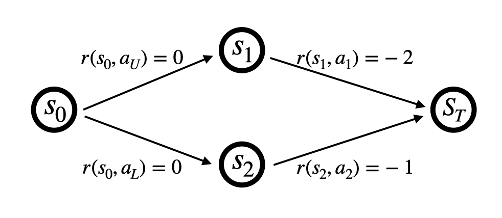
Figure 1: A diagnostic MDP from Gordon (1996). The state $s_{0}$ is the initial state with two actions $a_{U}$ and $a_{L}$ available, both of which yield a 0 reward. At $s_{1}$, only one action $a_{1}$ is available, which yields a reward -2. At $s_{2}$, the action $a_{2}$ yields a reward -1. Both $a_{1}$ and $a_{2}$ leads to the terminal state $S_{T}$.

We use a diagnostic MDP from Gordon (1996) (Figure 1) to illustrate the chattering of linear SARSA. Gordon (1996) tested the $\epsilon$-greedy policy (5), which is not continuous. We further test the $\epsilon$-softmax policy (6), whose Lipschitz constant is inversely proportional to the temperature $\iota$. When $\iota$ approaches $0$, the $\epsilon$-softmax policy approaches the $\epsilon$-greedy policy. We run Algorithm 1 in this MDP with $C_{\Gamma}=\infty$, i.e., there is no projection. Following Gordon (1996), we set $\epsilon=0.1,\gamma=1.0$, and $\alpha_{t}=0.01\,\forall t$. As discussed in Gordon (1996), using a smaller discount factor or a decaying learning rate only slows down the chattering but the chattering always occurs. Following Gordon (1996), we use the following feature function:

$$x(s_{0},a_{U}) =[1,0,0]^{\top},\,x(s_{0},a_{L})=[0,1,0]^{\top},$$ (51)

$$x(s_{1},a_{1}) =x(s_{2},a_{2})=[0,0,1]^{\top}.$$ (52)

In other words, it is essentially state aggregation.

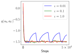
Figure 2: The action value of $a_{U}$ during training under different temperatures.

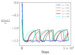
Figure 3: The $\alpha_{r}$-normalized action value of $a_{U}$ during training with a fixed temperature $\iota=0.01$. The reward of the MDP in Figure 1 is scaled via $\alpha_{r}$, e.g., the reward for the action $a_{1}$ is now $-2\alpha_{r}$.

As shown in Figure 2, when the temperature is small (i.e., $\iota=0.01$), linear SARSA chatters. We further fix $\iota$ to be $0.01$ and test reward with different magnitudes. To this end, we multiply the reward with a multiplier $\alpha_{r}$. We stress that this is just a simple way to get MDPs with rewards of different magnitudes. It does not mean that one should artificially scale the reward down when Theorem 4.4 does not apply. As shown in Figure 3, the chattering behavior disappears with $\alpha_{r}=0.1$. This suggests that our results might be improved such that when the magnitude of the rewards is small enough we can also achieve convergence to a fixed point, instead of a bounded region. We, however, leave this for future work. When we set $\alpha_{r}=4.0$, the iterates still only chatter but do not diverge. This suggests that our requirement for $r_{max}$ might be only sufficient and not necessary. We, however, leave the development of a necessary condition for future work. All the curves in Figures 2 and 3 are from a single run. Due to the randomness in the policy and the initialization of the weight, we find the peaks and valleys can sometimes average each other out when we average over multiple runs.

7 Conclusion

The behavior of linear SARSA is a long-standing open problem in the RL community. Despite the progress made in this work, there are still many open problems regarding the behavior of linear SARSA. To name a few: how does linear SARSA behave if the policy improvement operator is merely continuous but not Lipschitz continuous? How does linear SARSA behave if both the Lipschitz constant and the magnitude of the rewards are not small? Can we get a convergence rate without using any projection? We hope this work can draw more attention to the convergence of linear SARSA, arguably one of the most fundamental RL algorithms.

Appendix A Proofs of Section 3

A.1 Proof of Theorem 3.9

See 3.9

Proof.

We consider a Lyapunov function

$$M(x)\doteq\frac{1}{2}\norm{x}^{2}.$$ (53)

It is well-known that for any $x,x^{\prime}$,

$$M(x^{\prime})\leq M(x)+{\left<\nabla M(x),x^{\prime}-x\right>}+\frac{1}{2}\norm{x-x^{\prime}}^{2}.$$ (54)

Using $x^{\prime}=u_{t+1}-w^{*}_{\theta_{t+1}}$ and $x=\Gamma(u_{t})-w^{*}_{\theta_{t}}$ in the above inequality and recalling the update (33)

$$u_{t+1}= \Gamma(u_{t})+\alpha_{t}(F_{\theta_{t}}(\Gamma(u_{t}),Y_{t})-\Gamma(u_{t}))$$ (55)

$$= f_{\theta_{t}}^{\alpha_{t}}(\Gamma(u_{t}))+\alpha_{t}\left(F_{\theta_{t}}(\Gamma(u_{t}),Y_{t})-\bar{F}_{\theta_{t}}(\Gamma(u_{t}))\right)$$ (56)

yield

$$\frac{1}{2}\norm{u_{t+1}-w^{*}_{\theta_{t+1}}}^{2}$$ (57)

$$\leq \frac{1}{2}\norm{\Gamma(u_{t})-w^{*}_{\theta_{t}}}^{2}+{\left<\Gamma(u_{t})-w^{*}_{\theta_{t}},u_{t+1}-\Gamma(u_{t})+w^{*}_{\theta_{t}}-w^{*}_{\theta_{t+1}}\right>}$$ (58)

$$+\frac{1}{2}\norm{u_{t+1}-\Gamma(u_{t})+w^{*}_{\theta_{t}}-w^{*}_{\theta_{t+1}}}^{2}$$ (59)

$$= \frac{1}{2}\norm{\Gamma(u_{t})-w^{*}_{\theta_{t}}}^{2}$$ (60)

$$+\underbrace{{\left<\Gamma(u_{t})-w^{*}_{\theta_{t}},w^{*}_{\theta_{t}}-w^{*}_{\theta_{t+1}}\right>}}_{T_{1}}$$ (61)

$$+\underbrace{{\left<\Gamma(u_{t})-w^{*}_{\theta_{t}},f^{\alpha_{t}}_{\theta_{t}}(\Gamma(u_{t}))-\Gamma(u_{t})\right>}}_{T_{2}}$$ (62)

$$+\alpha_{t}\underbrace{{\left<\Gamma(u_{t})-w^{*}_{\theta_{t}},F_{\theta_{t}}(\Gamma(u_{t}),Y_{t})-\bar{F}_{\theta_{t}}(\Gamma(u_{t}))\right>}}_{T_{3}}$$ (63)

$$+\alpha_{t}^{2}\underbrace{\norm{F_{\theta_{t}}(\Gamma(u_{t}),Y_{t})-\Gamma(u_{t})}^{2}}_{T_{5}}$$ (64)

$$+\underbrace{\norm{w^{*}_{\theta_{t}}-w^{*}_{\theta_{t+1}}}^{2}}_{T_{6}}.$$ (65)

Here we do not have $T_{4}$ because the counterpart in Zhang et al. (2022) is now 0. To further decompose $T_{3}$, we define a function $\tau_{\alpha}$ of $\alpha$ as

$$\tau_{\alpha}\doteq\min\quantity{n\geq 0\mid C_{M}\tau^{n}\leq\alpha},$$ (66)

where the constants $C_{M}$ and $\tau$ are given in Lemma 3.3. In particular, $\tau_{\alpha_{t}}$ denotes the number of steps the chain needs to mix to an accuracy of $\alpha_{t}$. It is easy to see

$$\tau_{\alpha}=\mathcal{O}\left(-\log\alpha\right),\,\lim_{\alpha\to 0}\alpha\tau_{\alpha}=0.$$ (67)

We now decompose $T_{3}$ as

$$T_{3}= {\left<\Gamma(u_{t})-w^{*}_{\theta_{t}},F_{\theta_{t}}(\Gamma(u_{t}),Y_{t})-\bar{F}_{\theta_{t}}(\Gamma(u_{t}))\right>}$$ (68)

$$= \underbrace{{\left<\Gamma(u_{t})-w^{*}_{\theta_{t}}-\left(\Gamma(u_{t-\tau_{\alpha_{t}}})-w^{*}_{\theta_{t-\tau_{\alpha_{t}}}}\right),F_{\theta_{t}}(\Gamma(u_{t}),Y_{t})-\bar{F}_{\theta_{t}}(\Gamma(u_{t}))\right>}}_{T_{31}}$$ (69)

$$+\underbrace{{\left<\Gamma(u_{t-\tau_{\alpha_{t}}})-w^{*}_{\theta_{t-\tau_{\alpha_{t}}}},F_{\theta_{t}}(\Gamma(u_{t}),Y_{t})-F_{\theta_{t}}(\Gamma(u_{t-\tau_{\alpha_{t}}}),Y_{t})+\bar{F}_{\theta_{t}}(\Gamma(u_{t-\tau_{\alpha_{t}}}))-\bar{F}_{\theta_{t}}(\Gamma(u_{t}))\right>}}_{T_{32}}$$ (70)

$$+\underbrace{{\left<\Gamma(u_{t-\tau_{\alpha_{t}}})-w^{*}_{\theta_{t-\tau_{\alpha_{t}}}},F_{\theta_{t}}(\Gamma(u_{t-\tau_{\alpha_{t}}}),Y_{t})-\bar{F}_{\theta_{t}}(\Gamma(u_{t-\tau_{\alpha_{t}}}))\right>}}_{T_{33}}.$$ (71)

We further decompose $T_{33}$ as

$$T_{33}= {\left<\Gamma(u_{t-\tau_{\alpha_{t}}})-w^{*}_{\theta_{t-\tau_{\alpha_{t}}}},F_{\theta_{t}}(\Gamma(u_{t-\tau_{\alpha_{t}}}),Y_{t})-\bar{F}_{\theta_{t}}(\Gamma(u_{t-\tau_{\alpha_{t}}}))\right>}$$ (72)

$$= \underbrace{{\left<\Gamma(u_{t-\tau_{\alpha_{t}}})-w^{*}_{\theta_{t-\tau_{\alpha_{t}}}},F_{\theta_{t-\tau_{\alpha_{t}}}}(\Gamma(u_{t-\tau_{\alpha_{t}}}),\tilde{Y}_{t})-\bar{F}_{\theta_{t-\tau_{\alpha_{t}}}}(\Gamma(u_{t-\tau_{\alpha_{t}}}))\right>}}_{T_{331}}+$$ (73)

$$\underbrace{{\left<\Gamma(u_{t-\tau_{\alpha_{t}}})-w^{*}_{\theta_{t-\tau_{\alpha_{t}}}},F_{\theta_{t-\tau_{\alpha_{t}}}}(\Gamma(u_{t-\tau_{\alpha_{t}}}),Y_{t})-F_{\theta_{t-\tau_{\alpha_{t}}}}(\Gamma(u_{t-\tau_{\alpha_{t}}}),\tilde{Y}_{t})\right>}}_{T_{332}}+$$ (74)

$$\underbrace{{\left<\Gamma(u_{t-\tau_{\alpha_{t}}})-w^{*}_{\theta_{t-\tau_{\alpha_{t}}}},F_{\theta_{t}}(\Gamma(u_{t-\tau_{\alpha_{t}}}),Y_{t})-F_{\theta_{t-\tau_{\alpha_{t}}}}(\Gamma(u_{t-\tau_{\alpha_{t}}}),Y_{t})\right>}}_{T_{333}}+$$ (75)

$$\underbrace{{\left<\Gamma(u_{t-\tau_{\alpha_{t}}})-w^{*}_{\theta_{t-\tau_{\alpha_{t}}}},\bar{F}_{\theta_{t-\tau_{\alpha_{t}}}}(\Gamma(u_{t-\tau_{\alpha_{t}}}))-\bar{F}_{\theta_{t}}(\Gamma(u_{t-\tau_{\alpha_{t}}}))\right>}}_{T_{334}}.$$ (76)

Here $\quantity{\tilde{Y}_{t}}$ is an auxiliary chain inspired from Zou et al. (2019). Before time $t-\tau_{\alpha_{t}}-1$, $\quantity{\tilde{Y}_{t}}$ is exactly the same as $\quantity{Y_{t}}$. After time $t-\tau_{\alpha_{t}}-1$, $\tilde{Y}_{t}$ evolves according to the fixed kernel $P_{\theta_{t-\tau_{\alpha_{t}}}}$ while $Y_{t}$ evolves according the changing kernel $P_{\theta_{t-\tau_{\alpha_{t}}}},P_{\theta_{k-\tau_{\alpha_{t}}+1}},\dots$.

$$\quantity{\tilde{Y}_{t}} :\dots\to Y_{t-\tau_{\alpha_{t}}-1}\underbrace{\to}_{P_{\theta_{t-\tau_{\alpha_{t}}}}}Y_{t-\tau_{\alpha_{t}}}\underbrace{\to}_{P_{\theta_{t-\tau_{\alpha_{t}}}}}\tilde{Y}_{t-\tau_{\alpha_{t}}+1}\underbrace{\to}_{P_{\theta_{t-\tau_{\alpha_{t}}}}}\tilde{Y}_{t-\tau_{\alpha_{t}}+2}\to\dots$$ (77)

$$\quantity{Y_{t}} :\dots\to Y_{t-\tau_{\alpha_{t}}-1}\underbrace{\to}_{P_{\theta_{t-\tau_{\alpha_{t}}}}}Y_{t-\tau_{\alpha_{t}}}\underbrace{\to}_{P_{\theta_{t-\tau_{\alpha_{t}}+1}}}Y_{t-\tau_{\alpha_{t}}+1}\underbrace{\to}_{P_{\theta_{t-\tau_{\alpha_{t}}+2}}}Y_{t-\tau_{\alpha_{t}}+2}\to\dots.$$ (78)

We are now ready to present bounds for each of the above terms. To begin, we define some shorthand:

$$A \doteq 2L_{F}+1,\quad B\doteq U_{F},\quad C\doteq AU_{w}+B+A+A(1+U_{F}^{\prime}+U_{F}^{\prime\prime}),\,\alpha_{i:j}\doteq\sum_{t=i}^{j}\alpha_{t}.$$ (79)

According to (67), we can select a sufficiently large $t_{0}$ such that

$$\alpha_{t-\tau_{\alpha_{t}},t-1}\leq\frac{1}{4A}$$ (80)

holds for all $t$. This condition is crucial for Lemma C.2, which plays an important role in the following bounds.

Lemma A.1.

(Bound of $T_{1}$)

$$T_{1}\leq L_{w}L_{\theta}\alpha_{t}\norm{\Gamma(u_{t})-w^{*}_{\theta_{t}}}.$$ (81)

The proof of Lemma A.1 is provided in Section D.1.

Lemma A.2.

(Bound of $T_{2}$)

$$T_{2}\leq-(1-\kappa_{\alpha_{t}})\norm{\Gamma(u_{t})-w^{*}_{\theta_{t}}}^{2}.$$ (82)

The proof of Lemma A.2 is provided in Section D.2.

Lemma A.3.

(Bound of $T_{31}$)

$$T_{31}\leq 8(L_{w}L_{\theta}+1)\alpha_{t-\tau_{\alpha_{t}},t-1}\left(A^{2}\norm{\Gamma(u_{t})-w^{*}_{\theta_{t}}}^{2}+C^{2}\right).$$ (83)

The proof of Lemma A.3 is provided in Section D.3.

Lemma A.4.

(Bound of $T_{32}$)

$$T_{32}\leq 16\alpha_{t-\tau_{\alpha_{t}},t-1}(1+L_{w}L_{\theta}\alpha_{t-\tau_{\alpha_{t}},t-1})\left(A^{2}\norm{\Gamma(u_{t})-w^{*}_{\theta_{t}}}^{2}+C^{2}\right).$$ (84)

The proof of Lemma A.4 is provided in Section D.4.

Lemma A.5.

(Bound of $T_{331}$)

$$\mathbb{E}\left[T_{331}\right]\leq \frac{8\alpha_{t}(1+L_{w}L_{\theta}\alpha_{t-\tau_{\alpha_{t}},t-1})}{A}\left(A^{2}\mathbb{E}\left[\norm{\Gamma(u_{t})-w^{*}_{\theta_{t}}}^{2}\right]+C^{2}\right).$$ (85)

The proof of Lemma A.5 is provided in Section D.5.

Lemma A.6.

(Bound of $T_{332}$)

$$\mathbb{E}\left[T_{332}\right]\leq\frac{8{|\mathcal{Y}|}L_{P}L_{\theta}\sum_{j=t-\tau_{\alpha_{t}}}^{t-1}\alpha_{t-\tau_{\alpha_{t}},j}(1+L_{w}L_{\theta}\alpha_{t-\tau_{\alpha_{t}},t-1})}{A}\left(A^{2}\mathbb{E}\left[\norm{\Gamma(u_{t})-w^{*}_{\theta_{t}}}^{2}\right]+C^{2}\right).$$ (86)

The proof of Lemma A.6 is provided in Section D.6.

Lemma A.7.

(Bound of $T_{333}$)

$$T_{333}\leq\frac{4L_{F}^{\prime}L_{\theta}\alpha_{t-\tau_{\alpha_{t}},t-1}(1+L_{w}L_{\theta}\alpha_{t-\tau_{\alpha_{t}},t-1})}{A^{2}}\left(A^{2}\norm{\Gamma(u_{t})-w^{*}_{\theta_{t}}}^{2}+C^{2}\right).$$ (87)

The proof of Lemma A.7 is provided in Section D.7.

Lemma A.8.

(Bound of $T_{334}$)

$$T_{334}\leq\frac{4L_{F}^{\prime\prime}L_{\theta}\alpha_{t-\tau_{\alpha_{t}},t-1}(1+L_{w}L_{\theta}\alpha_{t-\tau_{\alpha_{t}},t-1})}{A^{2}}\left(A^{2}\norm{\Gamma(u_{t})-w^{*}_{\theta_{t}}}^{2}+C^{2}\right).$$ (88)

The proof of Lemma A.8 is provided in Section D.8.

Lemma A.9.

(Bound of $T_{5}$)

$$T_{5}\leq 2\left(A^{2}\norm{\Gamma(u_{t})-w^{*}_{\theta_{t}}}^{2}+C^{2}\right).$$ (89)

The proof of Lemma A.9 is provided in Section D.9.

Lemma A.10.

(Bound of $T_{6}$)

$$T_{6}=\norm{w^{*}_{\theta_{t}}-w^{*}_{\theta_{t+1}}}^{2}\leq L_{w}^{2}L_{\theta}^{2}\alpha_{t}^{2}.$$ (90)

Lemma A.10 follows immediately from Lemma C.5.

We now assemble the bounds in Lemmas A.1 - A.10 back into (57). Define

$$L_{\alpha,t}\doteq \left(\sum_{j=t-\tau_{\alpha_{t}}}^{t}\alpha_{t-\tau_{\alpha_{t}},j}\right)(1+L_{w}L_{\theta}\max\quantity{1,\alpha_{t-\tau_{\alpha_{t}},t}}),$$ (91)

$$C_{0}\doteq \max\quantity{A^{2},C^{2}}\max\quantity{16,L_{w}^{2}L_{\theta}^{2},8{|\mathcal{Y}|}L_{P}L_{\theta},4L_{F}^{\prime}L_{\theta},4L_{F}^{\prime\prime}L_{\theta}},$$ (92)

Using $A>1$ and Lemmas A.3 - A.10, it is easy to see

$$\mathbb{E}\left[T_{3}\right]\leq C_{0}L_{\alpha,t}\left(\mathbb{E}\left[\norm{\Gamma(u_{t})-w^{*}_{\theta_{t}}}^{2}\right]+1\right),$$ (93)

$$\alpha_{t}\mathbb{E}\left[T_{3}\right]\leq C_{0}\alpha_{t}L_{\alpha,t}\left(\mathbb{E}\left[\norm{\Gamma(u_{t})-w^{*}_{\theta_{t}}}^{2}\right]+1\right),$$ (94)

$$\mathbb{E}\left[T_{5}\right]\leq C_{0}\left(\mathbb{E}\left[\norm{\Gamma(u_{t})-w^{*}_{\theta_{t}}}^{2}\right]+1\right),$$ (95)

$$\alpha_{t}^{2}\mathbb{E}\left[T_{5}\right]\leq C_{0}\alpha_{t}^{2}\left(\mathbb{E}\left[\norm{\Gamma(u_{t})-w^{*}_{\theta_{t}}}^{2}\right]+1\right),$$ (96)

$$\mathbb{E}\left[T_{6}\right]\leq C_{0}\alpha_{t}^{2}.$$ (97)

Then we have

$$\frac{1}{2}\mathbb{E}\left[\norm{u_{t+1}-w^{*}_{\theta_{t+1}}}^{2}\right]$$ (98)

$$\leq \frac{1}{2}\mathbb{E}\left[\norm{\Gamma(u_{t})-w^{*}_{\theta_{t}}}^{2}\right]+L_{w}L_{\theta}\alpha_{t}\mathbb{E}\left[\norm{\Gamma(u_{t})-w^{*}_{\theta_{t}}}\right]-(1-\kappa_{\alpha_{t}})\mathbb{E}\left[\norm{\Gamma(u_{t})-w^{*}_{\theta_{t}}}^{2}\right]$$ (99)

$$+C_{0}\alpha_{t}L_{\alpha,t}\left(\mathbb{E}\left[\norm{\Gamma(u_{t})-w^{*}_{\theta_{t}}}^{2}\right]+1\right)+C_{0}\alpha_{t}^{2}\left(\mathbb{E}\left[\norm{\Gamma(u_{t})-w^{*}_{\theta_{t}}}^{2}\right]+1\right)$$ (100)

$$+C_{0}\alpha_{t}^{2},$$ (101)

implying

$$\mathbb{E}\left[\norm{u_{t+1}-w^{*}_{\theta_{t+1}}}^{2}\right]\leq \left(1-2\left(1-\kappa_{\alpha_{t}}-C_{0}\alpha_{t}L_{\alpha,t}-C_{0}\alpha_{t}^{2}\right)\right)\mathbb{E}\left[\norm{\Gamma(u_{t})-w^{*}_{\theta_{t}}}^{2}\right]$$ (102)

$$+2L_{w}L_{\theta}\alpha_{t}\mathbb{E}\left[\norm{\Gamma(u_{t})-w^{*}_{\theta_{t}}}\right]+2C_{0}\alpha_{t}L_{\alpha,t}+4C_{0}\alpha_{t}^{2}.$$ (103)

Observing that

$$L_{\alpha,t}=\mathcal{O}\left(\alpha_{t}\log^{2}\alpha_{t}\right)$$ (104)

then completes the proof. ∎

A.2 Proof of Corollary 3.10

See 3.10

Proof.

According to Theorem 3.9, we have

$$\mathbb{E}\left[\norm{u_{t+1}-w^{*}_{\theta_{t+1}}}^{2}\right]\leq \left(1-2\left(1-\kappa_{\alpha_{t}}-C_{0}\alpha_{t}L_{\alpha,t}-C_{0}\alpha_{t}^{2}\right)\right)\mathbb{E}\left[\norm{\Gamma(u_{t})-w^{*}_{\theta_{t}}}^{2}\right]$$ (105)

$$+2L_{w}L_{\theta}\alpha_{t}\mathbb{E}\left[\norm{\Gamma(u_{t})-w^{*}_{\theta_{t}}}\right]+2C_{0}\alpha_{t}L_{\alpha,t}+4C_{0}\alpha_{t}^{2}.$$ (106)

Since $L_{\alpha,t}=\mathcal{O}\left(\alpha_{t}\log^{2}\alpha_{t}\right)$, we conclude that there exists a constant $C_{1}>0$ such that

$$\mathbb{E}\left[\norm{u_{t+1}-w^{*}_{\theta_{t+1}}}^{2}\right]\leq \left(1-2\left(1-\sqrt{1-\eta\alpha_{t}}-C_{1}\alpha_{t}^{2}\log^{2}\alpha_{t}\right)\right)\mathbb{E}\left[\norm{\Gamma(u_{t})-w^{*}_{\theta_{t}}}^{2}\right]$$ (107)

$$+2L_{w}L_{\theta}\alpha_{t}\mathbb{E}\left[\norm{\Gamma(u_{t})-w^{*}_{\theta_{t}}}\right]+C_{1}\alpha_{t}^{2}\log^{2}\alpha_{t}.$$ (108)

When $t_{0}$ is sufficiently large, we have $\forall t$,

$$1-2\left(1-\sqrt{1-\eta\alpha_{t}}-C_{1}\alpha_{t}^{2}\log^{2}\alpha_{t}\right)>0.$$ (109)

Using

$$\norm{\Gamma(u_{t})-w^{*}_{\theta_{t}}}=\norm{\Gamma(u_{t})-\Gamma(w^{*}_{\theta_{t}})}\leq\norm{u_{t}-w^{*}_{\theta_{t}}}$$ (110)

then yields

$$\mathbb{E}\left[\norm{u_{t+1}-w^{*}_{\theta_{t+1}}}^{2}\right]$$ (111)

$$\leq \left(1-2\left(1-\sqrt{1-\eta\alpha_{t}}-C_{1}\alpha_{t}^{2}\log^{2}\alpha_{t}\right)\right)\mathbb{E}\left[\norm{u_{t}-w^{*}_{\theta_{t}}}^{2}\right]$$ (112)

$$+2L_{w}L_{\theta}\alpha_{t}\mathbb{E}\left[\norm{u_{t}-w^{*}_{\theta_{t}}}\right]+C_{1}\alpha_{t}^{2}\log^{2}\alpha_{t}$$ (113)

$$\leq \left(1-2\left(1-\sqrt{1-\eta\alpha_{t}}-C_{1}\alpha_{t}^{2}\log^{2}\alpha_{t}\right)\right)\mathbb{E}\left[\norm{u_{t}-w^{*}_{\theta_{t}}}^{2}\right]$$ (114)

$$+2L_{w}L_{\theta}\alpha_{t}\sqrt{\mathbb{E}\left[\norm{u_{t}-w^{*}_{\theta_{t}}}^{2}\right]}+C_{1}\alpha_{t}^{2}\log^{2}\alpha_{t}\mbox{\quad(Jensen's inequality)\quad}.$$ (115)

Since

$$\lim_{\alpha\to 0}\frac{1-\sqrt{1-\eta\alpha}}{\frac{\eta}{2}\alpha}=1,$$ (116)

we conclude that when $t_{0}$ is sufficiently large, $\forall t$,

$$1-\sqrt{1-\eta\alpha_{t}}-C_{1}\alpha_{t}^{2}\log^{2}\alpha_{t}\geq\frac{\eta}{3}\alpha_{t}-C_{1}\alpha_{t}^{2}\log^{2}\alpha_{t}^{2}\geq\frac{\eta}{4}\alpha_{t}.$$ (117)

With

$$z_{t}\doteq\sqrt{\mathbb{E}\left[\norm{u_{t}-w^{*}_{\theta_{t}}}^{2}\right]},$$ (118)

we then get

$$z_{t+1}^{2}\leq\left(1-\frac{\eta}{2}\alpha_{t}\right)z_{t}^{2}+2L_{w}L_{\theta}\alpha_{t}z_{t}+C_{1}\alpha_{t}^{2}\log^{2}\alpha_{t}.$$ (119)

If

$$\left(1-\frac{\eta}{2}\alpha_{t}\right)z_{t}^{2}+2L_{w}L_{\theta}\alpha_{t}z_{t} \leq(1-\frac{\eta}{3}\alpha_{t})z_{t}^{2},$$ (120)

$$\iff\frac{12L_{w}L_{\theta}}{\eta} \leq z_{t},$$ (121)

we have

$$z_{t+1}^{2}\leq(1-\frac{\eta}{3}\alpha_{t})z_{t}^{2}+C_{1}\alpha_{t}^{2}\log^{2}\alpha_{t}.$$ (122)

If

$$\frac{12L_{w}L_{\theta}}{\eta} \geq z_{t},$$ (123)

we have

$$z_{t+1}^{2}\leq \left(1-\frac{\eta}{2}\alpha_{t}\right)z_{t}^{2}+2L_{w}L_{\theta}\alpha_{t}z_{t}+C_{1}\alpha_{t}^{2}\log^{2}\alpha_{t}$$ (124)

$$\leq \left(1-\frac{\eta}{2}\alpha_{t}\right)z_{t}^{2}+\frac{24L_{w}^{2}L_{\theta}^{2}}{\eta}\alpha_{t}+C_{1}\alpha_{t}^{2}\log^{2}\alpha_{t}.$$ (125)

Since for any time $t$, one of (121) and (123) must hold, we always have

$$z_{t+1}^{2}\leq \left(1-\frac{\eta}{3}\alpha_{t}\right)z_{t}^{2}+\frac{24L_{w}^{2}L_{\theta}^{2}}{\eta}\alpha_{t}+C_{1}\alpha_{t}^{2}\log^{2}\alpha_{t}.$$ (126)

Telescoping the above inequality from $t_{0}$ to $t$ yields

$$z_{t}^{2}\leq \underbrace{\prod_{i=t_{0}}^{t-1}\left(1-\frac{\eta}{3}\alpha_{i}\right)}_{E_{1}}z_{t_{0}}^{2}+\frac{24L_{w}^{2}L_{\theta}^{2}}{\eta}\underbrace{\sum_{i=t_{0}}^{t-1}\prod_{j=i+1}^{t-1}\left(1-\frac{\eta}{3}\alpha_{j}\right)\alpha_{i}}_{E_{2}}$$ (127)

$$+C_{1}\underbrace{\sum_{i=t_{0}}^{t-1}\prod_{j=i+1}^{t-1}\left(1-\frac{\eta}{3}\alpha_{j}\right)\alpha_{i}^{2}\log^{2}\alpha_{i}}_{E_{3}},$$ (128)

where we adopt the convention that $\prod_{x=i}^{j}\left(\cdot\right)=1$ if $i>j$. For $E_{1}$, using $1+x\leq\exp x$ yields

$$E_{1}\leq \exp\left(-\frac{\eta}{3}\sum_{i=t_{0}}^{t-1}\alpha_{i}\right)\leq\exp\left(-\frac{\eta}{3}\int_{x=t_{0}}^{t}\frac{c_{\alpha}}{(t_{0}+x)^{\epsilon_{\alpha}}}dx\right)$$ (129)

$$= \begin{cases}\left(\frac{2t_{0}}{t_{0}+t}\right)^{\frac{\eta c_{\alpha}}{3}},&\epsilon_{\alpha}=1\\ \exp\left(\frac{\eta c_{\alpha}}{3(1-\epsilon_{\alpha})}\left((2t_{0})^{1-\epsilon_{\alpha}}-(t_{0}+t)^{1-\epsilon_{\alpha}}\right)\right),&\epsilon_{\alpha}\in(0,1)\end{cases}.$$ (130)

For $E_{2}$, define

$$B_{t}\doteq\sum_{i=0}^{t}\prod_{j=i+1}^{t}\left(1-\frac{\eta}{3}\alpha_{j}\right)\alpha_{i}.$$ (131)

Then we have

$$B_{t}=\alpha_{t}+(1-\frac{\eta}{3}\alpha_{t})B_{t-1}.$$ (132)

When $t_{0}$ is sufficiently large such that

$$1-\frac{\eta}{3}\alpha_{t}>0,$$ (133)

it is easy to see

$$B_{t-1}\leq\frac{3}{\eta}\implies B_{t}\leq\frac{3}{\eta}.$$ (134)

As $B_{0}=\alpha_{0}$, we have $B_{0}<\frac{3}{\eta}$ for sufficiently large $t_{0}$. We, therefore, conclude by induction that $\forall t$,

$$B_{t}\leq\frac{3}{\eta}.$$ (135)

Consequently,

$$E_{2}\leq B_{t-1}\leq\frac{3}{\eta}.$$ (136)

For $E_{3}$, we have

$$E_{3}\leq \log^{2}\alpha_{t}\underbrace{\sum_{i=t_{0}}^{t-1}\prod_{j=i+1}^{t-1}\left(1-\frac{\eta}{3}\alpha_{j}\right)\alpha_{i}^{2}}_{E_{4}}.$$ (137)

If $\epsilon_{\alpha}=1$, we have

$$E_{4}\leq \sum_{i=t_{0}}^{t-1}\exp\left(-\frac{\eta}{3}\int_{x=i+1}^{t}\frac{c_{\alpha}}{(t_{0}+x)^{\epsilon_{\alpha}}}dx\right)\frac{c_{\alpha}^{2}}{(t_{0}+i)^{2\epsilon_{\alpha}}}$$ (138)

$$= \sum_{i=t_{0}}^{t-1}\left(\frac{t_{0}+i+1}{t+t_{0}}\right)^{\frac{\eta c_{\alpha}}{3}}\frac{c_{\alpha}^{2}}{(t_{0}+i)^{2}}$$ (139)

$$= \sum_{i=t_{0}}^{t-1}\left(\frac{t_{0}+i+1}{t+t_{0}}\right)^{\frac{\eta c_{\alpha}}{3}}\frac{c_{\alpha}^{2}}{(t_{0}+i+1)^{2}}\left(\frac{t_{0}+i+1}{t_{0}+i}\right)^{2}$$ (140)

$$\leq \frac{4c_{\alpha}^{2}}{(t+t_{0})^{\frac{\eta c_{\alpha}}{3}}}\sum_{i=t_{0}}^{t-1}\frac{1}{(t_{0}+i+1)^{2-\frac{\eta c_{\alpha}}{3}}}$$ (141)

$$= \begin{cases}\mathcal{O}\left(t^{-\frac{\eta c_{\alpha}}{3}}\right),&\eta c_{\alpha}\in(0,3)\\ \mathcal{O}\left(\frac{\log t}{t}\right),&\eta c_{\alpha}=3\\ \mathcal{O}\left(\frac{1}{t}\right),&\eta c_{\alpha}\in(3,\infty)\end{cases}.$$ (142)

If $\epsilon_{\alpha}\in(0,1)$, when $t_{0}$ is sufficiently large, we can use induction (see, e.g., Section A.3.7 of Chen et al. (2021)) to show that

$$E_{4}=\mathcal{O}\left(\frac{1}{t^{\epsilon_{\alpha}}}\right).$$ (143)

Putting the bounds in (129) , (136), and (137) back into (126) yields

$$z_{t}^{2}=\frac{72L_{w}^{2}L_{\theta}^{2}}{\eta^{2}}+\begin{cases}\mathcal{O}\left(t^{-\frac{\eta c_{\alpha}}{3}}\log^{2}t\right),&\epsilon_{\alpha}=1,\eta c_{\alpha}\in(0,3)\\ \mathcal{O}\left(\frac{\log^{3}t}{t}\right),&\epsilon_{\alpha}=1,\eta c_{\alpha}=3\\ \mathcal{O}\left(\frac{\log^{2}t}{t}\right),&\epsilon_{\alpha}=1,\eta c_{\alpha}\in(3,\infty)\\ \mathcal{O}\left(\frac{\log^{2}t}{t^{\epsilon_{\alpha}}}\right),&\epsilon_{\alpha}\in(0,1)\end{cases}.$$ (144)

Here we have used the fact that $E_{3}$ always dominates $E_{1}$ for any $\epsilon_{\alpha},c_{\alpha}$. Using

$$\mathbb{E}\left[\norm{w_{t}-w^{*}_{w_{t}}}^{2}\right]=\mathbb{E}\left[\norm{\Gamma(u_{t})-\Gamma(w^{*}_{w_{t}})}^{2}\right]\leq\mathbb{E}\left[\norm{u_{t}-w^{*}_{w_{t}}}^{2}\right]=z_{t}^{2}$$ (145)

then completes the proof. ∎

Appendix B Proofs of Section 4

B.1 Proof of Theorem 4.4

See 4.4

Proof.

To start with, define

$$\mathcal{Y} \doteq\quantity{(s,a,s^{\prime},a^{\prime})\mid s\in\mathcal{S},a\in\mathcal{A},s^{\prime}\in\mathcal{S},p(s^{\prime}|s,a)>0},$$ (146)

$$Y_{t} \doteq(S_{t},A_{t},S_{t+1},A_{t+1}),$$ (147)

$$y \doteq(s,a,s^{\prime},a^{\prime}),$$ (148)

$$\tilde{\pi}_{\theta}(a|s) \doteq\pi_{\Gamma(\theta)}(a|s),$$ (149)

$$P_{\theta}((s_{1},a_{1},s_{1}^{\prime},a_{1}^{\prime}),(s_{2},a_{2},s_{2}^{\prime},a_{2}^{\prime})) \doteq\begin{cases}0&(s_{1}^{\prime},a_{1}^{\prime})\neq(s_{2},a_{2})\\ p(s_{2}^{\prime}|s_{2},a_{2})\tilde{\pi}_{\theta}(a_{2}^{\prime}|s_{2}^{\prime})&(s_{1}^{\prime},a_{1}^{\prime})=(s_{2},a_{2})\end{cases},$$ (150)

$$F_{\theta}(w,y)\doteq \left(r(s,a)+\gamma x(s^{\prime},a^{\prime})^{\top}w-x(s,a)^{\top}w\right)x(s,a)+w.$$ (151)

Here our $F_{\theta}(w,y)$ is actually independent of $\theta$.

The update of $\quantity{w_{t}}$ in Algorithm 1 with $\lambda=0$ can then be expressed as

$$w_{t+1}=\Gamma\left(w_{t}+\alpha_{t}\left(F_{\theta_{t}}(w_{t},Y_{t})-w_{t}\right)\right).$$ (152)

According to the action selection rule for $A_{t+1}$ specified in Algorithm 1, we have

$$\Pr(Y_{t+1}=y)=P_{\theta_{t+1}}(Y_{t},y),$$ (153)

Assumption 3.1 is then fulfilled.

Assumption 3.2 is immediately implied by Assumption 4.2. In particular, for any $\theta$, the invariant distribution of the chain induced by $P_{\theta}$ is $d_{\tilde{\pi}_{\theta}}(s)\tilde{\pi}_{\theta}(a|s)p(s^{\prime}|s,a)\tilde{\pi}_{\theta}(a^{\prime}|s^{\prime})$.

For Assumption 3.4, it is easy to see

$$\bar{F}_{\theta}(w)= X^{\top}D_{\tilde{\pi}_{\theta}}(\gamma P_{\tilde{\pi}_{\theta}}-I)Xw+X^{\top}D_{\tilde{\pi}_{\theta}}r+w,$$ (154)

$$f^{\alpha}_{\theta}(w)= w+\alpha\left(X^{\top}D_{\tilde{\pi}_{\theta}}(\gamma P_{\tilde{\pi}_{\theta}}-I)Xw+X^{\top}D_{\tilde{\pi}_{\theta}}r\right).$$ (155)

Define

$$w^{*}_{\theta}\doteq-\left(X^{\top}D_{\tilde{\pi}_{\theta}}(\gamma P_{\tilde{\pi}_{\theta}}-I)X\right)^{-1}X^{\top}D_{\tilde{\pi}_{\theta}}r.$$ (156)

It is then easy to see that $w^{*}_{\theta}$ is the unique fixed point of $\bar{F}_{\theta}(w)$. The uniform pseudo-contraction is verified by Lemma C.6. In particular, we have

$$\kappa_{\alpha}\doteq \sqrt{1-\eta\alpha},$$ (157)

$$\eta\doteq (1-\gamma)\inf_{\theta}\lambda_{min}\left(X^{\top}D_{\pi_{\theta}}X\right)>0,$$ (158)

where $\lambda_{min}(\cdot)$ denotes the minimum eigenvalue of a symmetric positive definite matrix.

We now verify Assumption 3.5. To verify Assumption 3.5 (i), we have

$$\norm{F_{\theta}(w,y)-F_{\theta}(w^{\prime},y)}$$ (159)

$$\leq \norm{\gamma x(s,a)x(s^{\prime},a^{\prime})^{\top}-x(s,a)x(s,a)^{\top}+I}\norm{w-w^{\prime}}$$ (160)

$$\leq \underbrace{\left((1+\gamma)x_{max}^{2}+1\right)}_{L_{F}}\norm{w-w^{\prime}}.$$ (161)

Assumption 3.5 (ii) immediately holds since our $F_{\theta}(w,y)$ is independent of $\theta$.

To verify Assumption 3.5 (iii), we have

$$\norm{F_{\theta}(0,y)}=\norm{r(s,a)x(s,a)}\leq\underbrace{r_{max}x_{max}}_{U_{F}}.$$ (162)

To verify Assumption 3.5 (iv), we have

$$\norm{\bar{F}_{\theta}(w)-\bar{F}_{\theta^{\prime}}(w)}_{\infty}$$ (163)

$$= \norm{X^{\top}\left(D_{\tilde{\pi}_{\theta}}(\gamma P_{\tilde{\pi}_{\theta}}-I)-D_{\tilde{\pi}_{\theta^{\prime}}}(\gamma P_{\tilde{\pi}_{\theta^{\prime}}}-I)\right)Xw+X^{\top}\left(D_{\tilde{\pi}_{\theta}}-D_{\tilde{\pi}_{\theta^{\prime}}}\right)r}_{\infty}$$ (164)

$$\leq \norm{X}_{\infty}^{2}\norm{D_{\tilde{\pi}_{\theta}}(\gamma P_{\tilde{\pi}_{\theta}}-I)-D_{\tilde{\pi}_{\theta^{\prime}}}(\gamma P_{\tilde{\pi}_{\theta^{\prime}}}-I)}_{\infty}\norm{w}_{\infty}+\norm{X}_{\infty}\norm{D_{\tilde{\pi}_{\theta}}-D_{\tilde{\pi}_{\theta^{\prime}}}}_{\infty}\norm{r}_{\infty}.$$ (165)

Lemma C.3 asserts that $D_{\pi_{\theta}}$ is Lipschitz continuous in $\theta$. We then conclude, by Lemma C.1, that there exist positive constants $L_{DP}>0,L_{D}>0$ such that

$$\norm{D_{\pi_{\theta}}(\gamma P_{\pi_{\theta}}-I)-D_{\pi_{\theta^{\prime}}}(\gamma P_{\pi_{\theta^{\prime}}}-I)}_{\infty}\leq L_{DP}L_{\pi}\norm{\theta-\theta}_{\infty},$$ (166)

$$\norm{D_{\pi_{\theta}}-D_{\pi_{\theta^{\prime}}}}_{\infty}\leq L_{D}L_{\pi}\norm{\theta-\theta^{\prime}}_{\infty}.$$ (167)

Importantly, $L_{DP}$ and $L_{D}$ do not depend on $C_{\Gamma}$. It is then easy to see that

$$\norm{\bar{F}_{\theta}(w)-\bar{F}_{\theta^{\prime}}(w)}_{\infty}\leq \left(\norm{X}_{\infty}^{2}L_{DP}L_{\pi}\norm{w}_{\infty}+\norm{X}_{\infty}\norm{r}_{\infty}L_{D}L_{\pi}\right)\norm{\Gamma(\theta)-\Gamma(\theta^{\prime})}_{\infty}$$ (168)

$$\leq \left(\norm{X}_{\infty}^{2}L_{DP}L_{\pi}\norm{w}+\norm{X}_{\infty}\norm{r}_{\infty}L_{D}L_{\pi}\right)\norm{\Gamma(\theta)-\Gamma(\theta^{\prime})}$$ (169)

$$\leq \left(\norm{X}_{\infty}^{2}L_{DP}L_{\pi}\norm{w}+\norm{X}_{\infty}\norm{r}_{\infty}L_{D}L_{\pi}\right)\norm{\theta-\theta^{\prime}}.$$ (170)

It follow immediately that

$$\norm{\bar{F}_{\theta}(w)-\bar{F}_{\theta^{\prime}}(w)}\leq \sqrt{K}\left(\norm{X}_{\infty}^{2}L_{DP}L_{\pi}\norm{w}+\norm{X}_{\infty}\norm{r}_{\infty}L_{D}L_{\pi}\right)\norm{\theta-\theta^{\prime}}.$$ (171)

To verify Assumption 3.5 (v), we first use Lemma C.4 to get

$$\norm{\left(X^{\top}D_{\tilde{\pi}_{\theta}}(\gamma P_{\tilde{\pi}_{\theta}}-I)X\right)^{-1}-\left(X^{\top}D_{\tilde{\pi}_{\theta^{\prime}}}(\gamma P_{\tilde{\pi}_{\theta^{\prime}}}-I)X\right)^{-1}}_{\infty}$$ (172)

$$\leq \norm{\left(X^{\top}D_{\tilde{\pi}_{\theta}}(\gamma P_{\tilde{\pi}_{\theta}}-I)X\right)^{-1}}_{\infty}\norm{\left(X^{\top}D_{\tilde{\pi}_{\theta^{\prime}}}(\gamma P_{\tilde{\pi}_{\theta^{\prime}}}-I)X\right)^{-1}}_{\infty}$$ (173)

$$\times\norm{X^{\top}D_{\tilde{\pi}_{\theta}}(\gamma P_{\tilde{\pi}_{\theta}}-I)X-X^{\top}D_{\tilde{\pi}_{\theta^{\prime}}}(\gamma P_{\tilde{\pi}_{\theta^{\prime}}}-I)X}_{\infty}.$$ (174)

Thanks to Assumption 4.2, for any $\theta$,

$$\left(X^{\top}D_{\pi_{\theta}}(\gamma P_{\pi_{\theta}}-I)X\right)^{-1}$$ (175)

is well-defined. Since $\bar{\Lambda}_{\pi}$ is a compact set, we conclude, by the extreme value theorem, that there exists a constant $U_{inv}>0$, independent of $C_{\Gamma}$, such that

$$\sup_{\theta}\norm{\left(X^{\top}D_{\pi_{\theta}}(\gamma P_{\pi_{\theta}}-I)X\right)^{-1}}_{\infty}<U_{inv}.$$ (176)

Recalling that $\tilde{\pi}_{\theta}(a|s)=\pi_{\Gamma(\theta)}(a|s)$ then yields

$$\sup_{\theta}\norm{\left(X^{\top}D_{\tilde{\pi}_{\theta}}(\gamma P_{\tilde{\pi}_{\theta}}-I)X\right)^{-1}}_{\infty}<U_{inv}.$$ (177)

It then follows immediately that

$$\norm{\left(X^{\top}D_{\tilde{\pi}_{\theta}}(\gamma P_{\tilde{\pi}_{\theta}}-I)X\right)^{-1}-\left(X^{\top}D_{\tilde{\pi}_{\theta^{\prime}}}(\gamma P_{\tilde{\pi}_{\theta^{\prime}}}-I)X\right)^{-1}}_{\infty}\leq U_{inv}^{2}\norm{X}_{\infty}^{2}L_{DP}L_{\pi}\norm{\theta-\theta^{\prime}}_{\infty}.$$ (178)

It is also easy to see that

$$\norm{X^{\top}D_{\tilde{\pi}_{\theta}}r}_{\infty} \leq\norm{X}_{\infty}\norm{r}_{\infty},$$ (179)

$$\norm{X^{\top}D_{\tilde{\pi}_{\theta}}r-X^{\top}D_{\tilde{\pi}_{\theta^{\prime}}}r}_{\infty} \leq\norm{X}_{\infty}L_{D}L_{\pi}\norm{r}_{\infty}.$$ (180)

Using Lemma C.1 again yields

$$\norm{w^{*}_{\theta}-w^{*}_{\theta^{\prime}}}_{\infty}\leq\left(U_{inv}^{2}\norm{X}_{\infty}^{2}L_{DP}\norm{X}_{\infty}+U_{inv}\norm{X}_{\infty}L_{D}\right)L_{\pi}\norm{r}_{\infty}\norm{\theta-\theta^{\prime}}_{\infty}.$$ (181)

It follows immediately that

$$\norm{w^{*}_{\theta}-w^{*}_{\theta^{\prime}}}\leq\underbrace{\sqrt{K}\left(U_{inv}^{2}\norm{X}_{\infty}^{2}L_{DP}\norm{X}_{\infty}+U_{inv}\norm{X}_{\infty}L_{D}\right)L_{\pi}\norm{r}_{\infty}}_{L_{w}}\norm{\theta-\theta^{\prime}}.$$ (182)

To verify Assumption 3.5 (vi), we have

$$\sup_{\theta}\norm{w^{*}_{\theta}}_{\infty}\leq U_{inv}\norm{X}_{\infty}\norm{r}_{\infty}.$$ (183)

It follows immediately that

$$\sup_{\theta}\norm{w^{*}_{\theta}}\leq\underbrace{\sqrt{K}U_{inv}\norm{X}_{\infty}\norm{r}_{\infty}}_{U_{w}}.$$ (184)

Assumption 3.5 (vii) follows immediately from Assumption 4.1.

We now verify Assumption 3.6. Assumption 3.6 (i) is fulfilled by our selection of $C_{\Gamma}$. It is easy to see

$$\tilde{\pi}_{\theta}(a|s)=\tilde{\pi}_{\Gamma(\theta)}(a|s),$$ (185)

Assumption 3.6 (ii) then follows immediately.

With Assumptions 3.1 - 3.6 satisfied, we conclude by Corollary 3.10 that the iterates $\quantity{w_{t}}$ generated by Algorithm 1 with $\lambda=0$ satisfy

$$\mathbb{E}\left[\norm{w_{t}-w^{*}_{w_{t}}}^{2}\right]=\frac{72L_{w}^{2}L_{\theta}^{2}}{\eta^{2}}+\begin{cases}\mathcal{O}\left(t^{-\frac{\eta c_{\alpha}}{3}}\log^{2}t\right),&\epsilon_{\alpha}=1,\eta c_{\alpha}\in(0,3)\\ \mathcal{O}\left(\frac{\log^{3}t}{t}\right),&\epsilon_{\alpha}=1,\eta c_{\alpha}=3\\ \mathcal{O}\left(\frac{\log^{2}t}{t}\right),&\epsilon_{\alpha}=1,\eta c_{\alpha}\in(3,\infty)\\ \mathcal{O}\left(\frac{\log^{2}t}{t^{\epsilon_{\alpha}}}\right),&\epsilon_{\alpha}\in(0,1)\end{cases}.$$ (186)

where

$$L_{\theta}\doteq U_{F}+(L_{F}+1)C_{\Gamma}=\left(r_{max}x_{max}+\left((1+\gamma)x_{max}^{2}+2\right)C_{\Gamma}\right)$$ (187)

$$\leq 1+4C_{\Gamma}.$$ (188)

Consequently,

$$\mathbb{E}\left[\norm{w_{t}-w^{*}_{w_{t}}}\right]\leq \sqrt{\mathbb{E}\left[\norm{w_{t}-w^{*}_{w_{t}}}^{2}\right]}$$ (189)

$$= \frac{6\sqrt{2}L_{w}L_{\theta}}{\eta}+\begin{cases}\mathcal{O}\left(t^{-\frac{\eta c_{\alpha}}{6}}\log t\right),&\epsilon_{\alpha}=1,\eta c_{\alpha}\in(0,3)\\ \mathcal{O}\left(t^{-\frac{1}{2}}\log^{\frac{3}{2}}t\right),&\epsilon_{\alpha}=1,\eta c_{\alpha}=3\\ \mathcal{O}\left(t^{-\frac{1}{2}}\log t\right),&\epsilon_{\alpha}=1,\eta c_{\alpha}\in(3,\infty)\\ \mathcal{O}\left(t^{-\frac{\epsilon_{\alpha}}{2}}\log t\right),&\epsilon_{\alpha}\in(0,1)\end{cases}.$$ (190)

If

$$\norm{r}_{\infty}<\frac{1}{\sqrt{K}\left(U_{inv}^{2}\norm{X}_{\infty}^{2}L_{DP}\norm{X}_{\infty}+U_{inv}\norm{X}_{\infty}L_{D}\right)},$$ (191)

we get

$$L_{w}<1.$$ (192)

Since

$$\mathbb{E}\left[\norm{w_{t}-w_{*}}\right]$$ (193)

$$= \mathbb{E}\left[\norm{w_{t}-w^{*}_{w_{*}}}\right]$$ (194)

$$\leq \mathbb{E}\left[\norm{w_{t}-w^{*}_{w_{t}}}\right]+\mathbb{E}\left[\norm{w^{*}_{w_{t}}-w^{*}_{w_{*}}}\right]$$ (195)

$$\leq \mathbb{E}\left[\norm{w_{t}-w^{*}_{w_{t}}}\right]+L_{w}\mathbb{E}\left[\norm{w_{t}-w_{*}}\right],$$ (196)

we conclude that

$$\mathbb{E}\left[\norm{w_{t}-w_{*}}\right]\leq \frac{1}{1-L_{w}}\mathbb{E}\left[\norm{w_{t}-w^{*}_{w_{t}}}\right]$$ (197)

$$= \frac{6\sqrt{2}L_{w}\left(1+4C_{\Gamma}\right)}{\eta(1-L_{w})}+\begin{cases}\mathcal{O}\left(t^{-\frac{\eta c_{\alpha}}{6}}\log t\right),&\epsilon_{\alpha}=1,\eta c_{\alpha}\in(0,3)\\ \mathcal{O}\left(t^{-\frac{1}{2}}\log^{\frac{3}{2}}t\right),&\epsilon_{\alpha}=1,\eta c_{\alpha}=3\\ \mathcal{O}\left(t^{-\frac{1}{2}}\log t\right),&\epsilon_{\alpha}=1,\eta c_{\alpha}\in(3,\infty)\\ \mathcal{O}\left(t^{-\frac{\epsilon_{\alpha}}{2}}\log t\right),&\epsilon_{\alpha}\in(0,1)\end{cases},$$ (198)

which completes the proof.

∎

Appendix C Technical Lemmas

Lemma C.1.

Let $f_{1}(x),f_{2}(x)$ be two Lipschitz continuous functions with Lipschitz constants $L_{1},L_{2}$. Assume $\norm{f_{1}(x)}\leq U_{1},\norm{f_{2}(x)}\leq U_{2}$, then $L_{1}U_{2}+L_{2}U_{1}$ is a Lipschitz constant of $f(x)\doteq f_{1}(x)f_{2}(x)$.

Proof.

$$\norm{f_{1}(x)f_{2}(x)-f_{1}(y)f_{2}(y)}$$ (199)

$$\leq \norm{f_{1}(x)}\norm{f_{2}(x)-f_{2}(y)}+\norm{f_{2}(y)}\norm{f_{1}(x)-f_{1}(y)}$$ (200)

$$\leq (U_{1}L_{2}+U_{2}L_{1})\norm{x-y}.$$ (201)

∎

Lemma C.2.

Given positive integers $t_{1}<t_{2}$ satisfying

$$\alpha_{t_{1},t_{2}-1}\leq\frac{1}{4A},$$ (202)

we have, for any $t\in[t_{1},t_{2}]$,

$$\norm{\Gamma(u_{t})-\Gamma(u_{t_{1}})} \leq 2\alpha_{t_{1},t_{2}-1}(A\norm{\Gamma(u_{t_{1}})}+B),$$ (203)

$$\norm{\Gamma(u_{t})-\Gamma(u_{t_{1}})} \leq 4\alpha_{t_{1},t_{2}-1}(A\norm{\Gamma(u_{t_{2}})}+B),$$ (204)

$$\norm{\Gamma(u_{t})-\Gamma(u_{t_{1}})} \leq\min\quantity{\norm{\Gamma(u_{t_{1}})},\norm{\Gamma(u_{t_{2}})}}+\frac{B}{A}.$$ (205)

Proof.

Notice that

$$\norm{\Gamma(u_{t+1})}-\norm{\Gamma(u_{t})}$$ (206)

$$\leq \norm{\Gamma(u_{t+1})-\Gamma(u_{t})}$$ (207)

$$= \norm{\Gamma(u_{t+1})-\Gamma(\Gamma(u_{t}))}$$ (208)

$$\leq \norm{u_{t+1}-\Gamma(u_{t})}$$ (209)

$$= \alpha_{t}\norm{F_{\theta_{t}}(\Gamma(u_{t}),Y_{t})-\Gamma(u_{t})}$$ (210)

$$\leq \alpha_{t}\left(\norm{F_{\theta_{t}}(\Gamma(u_{t}),Y_{t})}+\norm{\Gamma(u_{t})}\right)$$ (211)

$$\leq \alpha_{t}(U_{F}+(L_{F}+1)\norm{\Gamma(u_{t})}\mbox{\quad(Lemma~{}\ref{lem bound of fxy})\quad}$$ (212)

$$\leq \alpha_{t}(A\norm{\Gamma(u_{t})}+B)\mbox{\quad(Using \eqref{eq shorthand a and b})\quad}$$ (213)

The rest of the proof follows from the proof of Lemma A.2 of Chen et al. (2021) up to changes of notations. We include it for completeness. Rearranging terms of the above inequality yields

$$\norm{\Gamma(u_{t+1})}+\frac{B}{A}\leq(1+\alpha_{t}A)\left(\norm{\Gamma(u_{t})}+\frac{B}{A}\right),$$ (214)

implying that for any $t\in(t_{1},t_{2}]$,

$$\norm{\Gamma(u_{t})}+\frac{B}{A}\leq\prod_{j=t_{1}}^{t-1}(1+A\alpha_{j})\left(\norm{\Gamma(u_{t_{1}})}+\frac{B}{A}\right).$$ (215)

Notice that for any $x\in[0,\frac{1}{2}]$, $1+x\leq\exp(x)\leq 1+2x$ always hold. Hence

$$\alpha_{t_{1},t_{2}-1}\leq\frac{1}{4A}$$ (216)

implies

$$\prod_{j=t_{1}}^{t-1}(1+A\alpha_{j})\leq\exp(A\alpha_{t_{1},t-1})\leq 1+2A\alpha_{t_{1},t-1}.$$ (217)

Consequently, for any $t\in(t_{1},t_{2}]$, we have

$$\norm{\Gamma(u_{t})}+\frac{B}{A} \leq\left(1+2A\alpha_{t_{1},t-1}\right)\left(\norm{\Gamma(u_{t_{1}})}+\frac{B}{A}\right)$$ (218)

$$\implies\norm{\Gamma(u_{t})} \leq\left(1+2A\alpha_{t_{1},t-1}\right)\norm{\Gamma(u_{t_{1}})}+2B\alpha_{t_{1},t-1},$$ (219)

which together with (213) yields that for any $t\in(t_{1},t_{2}-1]$

$$\norm{\Gamma(u_{t+1})-\Gamma(u_{t})} \leq\alpha_{t}\left(A\norm{\Gamma(u_{t})}+B\right)$$ (220)

$$\leq\alpha_{t}\left(A\left(1+2A\alpha_{t_{1},t-1}\right)\norm{\Gamma(u_{t_{1}})}+2AB\alpha_{t_{1},t-1}+B\right)$$ (221)

$$\leq 2\alpha_{t}(A\norm{\Gamma(u_{t_{1}})}+B)\mbox{\quad(Using $\alpha_{t_{1},t-1}\leq\frac{1}{4A}$)\quad}.$$ (222)

Consequently, for any $t\in(t_{1},t_{2}]$, we have

$$\norm{\Gamma(u_{t})-\Gamma(u_{t_{1}})} \leq\sum_{j=t_{1}}^{t-1}\norm{\Gamma(w_{j+1})-\Gamma(w_{j})}\leq\sum_{j=t_{1}}^{t-1}2\alpha_{j}(A\norm{\Gamma(u_{t_{1}})}+B)$$ (223)

$$=2\alpha_{t_{1},t-1}(A\norm{\Gamma(u_{t_{1}})}+B)\leq 2\alpha_{t_{1},t_{2}-1}(A\norm{\Gamma(u_{t_{1}})}+B),$$ (224)

which completes the proof of (203). For (204), we have from the above inequality

$$\norm{\Gamma(u_{t_{2}})-\Gamma(u_{t_{1}})}\leq 2\alpha_{t_{1},t_{2}-1}(A\norm{\Gamma(u_{t_{1}})}+B)$$ (225)

$$\leq 2\alpha_{t_{1},t_{2}-1}(A\norm{\Gamma(u_{t_{1}})-\Gamma(u_{t_{2}})}+A\norm{\Gamma(u_{t_{2}})}+B)$$ (226)

$$\leq \frac{1}{2}\norm{\Gamma(u_{t_{1}})-\Gamma(u_{t_{2}})}+2\alpha_{t_{1},t_{2}-1}(A\norm{\Gamma(u_{t_{2}})}+B),$$ (227)

implying

$$\norm{\Gamma(u_{t_{2}})-\Gamma(u_{t_{1}})}\leq 4\alpha_{t_{1},t_{2}-1}(A\norm{\Gamma(u_{t_{2}})}+B).$$ (228)

Consequently, for any $t\in[t_{1},t_{2}]$,

$$\norm{\Gamma(u_{t})-\Gamma(u_{t_{1}})}\leq 2\alpha_{t_{1},t_{2}-1}(A\norm{\Gamma(u_{t_{1}})}+B)$$ (229)

$$\leq 2\alpha_{t_{1},t_{2}-1}(A\norm{\Gamma(u_{t_{1}})-\Gamma(u_{t_{2}})}+A\norm{\Gamma(u_{t_{2}})}+B)$$ (230)

$$\leq 2\alpha_{t_{1},t_{2}-1}\left(A4\alpha_{t_{1},t_{2}-1}(A\norm{\Gamma(u_{t_{2}})}+B)+A\norm{\Gamma(u_{t_{2}})}+B\right)$$ (231)

$$\leq 4\alpha_{t_{1},t_{2}-1}(A\norm{\Gamma(u_{t_{2}})}+B)\mbox{\quad(Using $\alpha_{t_{1},t_{2}-1}\leq\frac{1}{4A}$)\quad},$$ (232)

which completes the proof of (204). (203) implies

$$\norm{\Gamma(u_{t})-\Gamma(u_{t_{1}})}\leq\norm{\Gamma(u_{t_{1}})}+\frac{B}{A},$$ (233)

(204) implies

$$\norm{\Gamma(u_{t})-\Gamma(u_{t_{1}})}\leq\norm{\Gamma(u_{t_{2}})}+\frac{B}{A},$$ (234)

then (205) follows immediately, which completes the proof. ∎

Lemma C.3.

Let Assumptions 4.1 and 4.2 hold. Then there exists a constant $L_{\pi}^{\prime}$ such that $\forall\theta,\theta^{\prime},a,s$,

$$\absolutevalue{d_{\pi_{\theta}}(s,a)-d_{\pi_{\theta^{\prime}}}(s,a)}\leq L_{\pi}^{\prime}\norm{\theta-\theta^{\prime}}_{\infty}.$$ (235)

Proof.

See, e.g., Lemma 9 of Zhang et al. (2021). ∎

Lemma C.4.

For any $\norm{\cdot}$, we have

$$\norm{X^{-1}-Y^{-1}}\leq\norm{X^{-1}}\norm{X-Y}\norm{Y^{-1}}.$$ (236)

Proof.

$$\norm{X^{-1}-Y^{-1}} =\norm{X^{-1}YY^{-1}-X^{-1}XY^{-1}}\leq\norm{X^{-1}}\norm{X-Y}\norm{Y^{-1}}.$$ (237)

∎

Lemma C.5.

Recall that

$$L_{\theta}=U_{F}+(L_{F}+1)C_{\Gamma},$$ (238)

then for any $j>i,y,y^{\prime},w$,

$$\norm{w^{*}_{\theta_{j}}-w^{*}_{\theta_{i}}}\leq L_{w}L_{\theta}\alpha_{i,j-1},$$ (239)

$$\absolutevalue{P_{\theta_{j}}(y,y^{\prime})-P_{\theta_{i}}(y,y^{\prime})}\leq L_{P}L_{\theta}\alpha_{i,j-1},$$ (240)

$$\norm{F_{\theta_{j}}(w,y)-F_{\theta_{i}}(w,y)}\leq L_{F}^{\prime}L_{\theta}\alpha_{i,j-1}\left(\norm{w}+U_{F}^{\prime}\right),$$ (241)

$$\norm{\bar{F}_{\theta_{j}}(w)-\bar{F}_{\theta_{i}}(w)}\leq L_{F}^{\prime\prime}L_{\theta}\alpha_{i,j-1}\left(\norm{w}+U_{F}^{\prime\prime}\right).$$ (242)

Proof.

$$\norm{w^{*}_{\theta_{j}}-w^{*}_{\theta_{i}}}\leq \sum_{k=i}^{j-1}\norm{w^{*}_{\theta_{k+1}}-w^{*}_{\theta_{k}}}$$ (243)

$$\leq \sum_{k=i}^{j-1}\norm{w^{*}_{\theta_{k+1}}-w^{*}_{\Gamma(\theta_{k})}}\mbox{\quad(Assumption~{}\ref{assu projection})\quad}$$ (244)

$$\leq \sum_{k=i}^{j-1}L_{w}\norm{\theta_{k+1}-\Gamma(\theta_{k})}$$ (245)

$$= \sum_{k=i}^{j-1}L_{w}\norm{w_{k+1}-\Gamma(w_{k})}$$ (246)

$$= \sum_{k=i}^{j-1}L_{w}\norm{\Gamma(u_{k+1})-\Gamma(\Gamma(u_{k}))}\mbox{\quad(Lemma~{}\ref{lem transform})\quad}$$ (247)

$$\leq \sum_{k=i}^{j-1}L_{w}\norm{u_{k+1}-\Gamma(u_{k})}$$ (248)

$$= \sum_{k=i}^{j-1}L_{w}\alpha_{k}\norm{F_{\theta_{k}}(\Gamma(u_{k}),Y_{k})-\Gamma(u_{k})}$$ (249)

$$\leq \sum_{k=i}^{j-1}L_{w}\alpha_{k}\left(U_{F}+L_{F}\norm{\Gamma(u_{k})}+\norm{\Gamma(u_{k})}\right)\mbox{\quad(Lemma~{}\ref{lem bound of fxy})\quad}$$ (250)

$$\leq \sum_{k=i}^{j-1}L_{w}\alpha_{k}\left(U_{F}+L_{F}C_{\Gamma}+C_{\Gamma}\right)$$ (251)

$$= L_{w}L_{\theta}\alpha_{i,j-1}.$$ (252)

Similarly we can get

$$\absolutevalue{P_{\theta_{j}}(y,y^{\prime})-P_{\theta_{i}}(y,y^{\prime})}\leq L_{P}L_{\theta}\alpha_{i,j-1}.$$ (253)

Moreover,

$$\norm{F_{\theta_{j}}(w,y)-F_{\theta_{i}}(w,y)}\leq \sum_{k=i}^{j-1}\norm{F_{\theta_{k+1}}(w,y)-F_{\theta_{k}}(w,y)}$$ (254)

$$\leq \sum_{k=i}^{j-1}\norm{F_{\theta_{k+1}}(w,y)-F_{\Gamma(\theta_{k})}(w,y)}\mbox{\quad(Assumption~{}\ref{assu projection})\quad}$$ (255)

$$\leq \sum_{k=i}^{j-1}L_{F}^{\prime}\norm{\theta_{k+1}-\Gamma(\theta_{k})}\left(\norm{w}+U_{F}^{\prime}\right)$$ (256)

$$\leq L_{F}^{\prime}L_{\theta}\alpha_{i,j-1}\left(\norm{w}+U_{F}^{\prime}\right).$$ (257)

Since $P_{\theta}=P_{\Gamma(\theta)}$, it is easy to see $d_{\theta}(y)=d_{\Gamma(\theta)}(y)$. Consequently, $\bar{F}_{\theta}(w)=\bar{F}_{\Gamma(\theta)}(w)$. We can then similarly get

$$\norm{\bar{F}_{\theta_{j}}(w)-\bar{F}_{\theta_{i}}(w)}\leq L_{F}^{\prime\prime}L_{\theta}\alpha_{i,j-1}\left(\norm{w}+U_{F}^{\prime\prime}\right),$$ (258)

which completes the proof. ∎

Lemma C.6.

(Lemma 5.4 of De Farias & Van Roy (2000)) There exists an $\bar{\alpha}$ such that for all $\alpha\in(0,\bar{\alpha})$ and all $\theta$,

$$\norm{f^{\alpha}_{\theta}(w)-w^{*}_{\theta}}\leq\kappa_{\alpha}\norm{w-w^{*}_{\theta}},$$ (259)

where

$$\kappa_{\alpha}\doteq\sqrt{1-(1-\gamma)\inf_{\theta}\lambda_{min}\left(X^{\top}D_{\pi_{\theta}}X\right)\alpha}<1.$$ (260)

Here $\lambda_{min}(\cdot)$ denotes the minimum eigenvalue of a symmetric positive definite matrix.

Proof.

The proof is due to De Farias & Van Roy (2000); we rewrite it in our notation for completeness. We first recall

$$f^{\alpha}_{\theta}(w)= w+\alpha\left(X^{\top}D_{\tilde{\pi}_{\theta}}(\gamma P_{\tilde{\pi}_{\theta}}-I)Xw+X^{\top}D_{\tilde{\pi}_{\theta}}r\right),$$ (261)

$$w^{*}_{\theta}= -\left(X^{\top}D_{\tilde{\pi}_{\theta}}(\gamma P_{\tilde{\pi}_{\theta}}-I)X\right)^{-1}X^{\top}D_{\tilde{\pi}_{\theta}}r.$$ (262)

Define

$$g_{\theta}(w)\doteq X^{\top}D_{\tilde{\pi}_{\theta}}(\gamma P_{\tilde{\pi}_{\theta}}-I)Xw+X^{\top}D_{\tilde{\pi}_{\theta}}r$$ (263)

$$= X^{\top}D_{\tilde{\pi}_{\theta}}X\left(X^{\top}D_{\tilde{\pi}_{\theta}}X\right)^{-1}X^{\top}D_{\tilde{\pi}_{\theta}}\left(\mathcal{T}_{\tilde{\pi}_{\theta}}Xw-Xw\right)$$ (264)

$$= X^{\top}D_{\tilde{\pi}_{\theta}}\Pi_{D_{\tilde{\pi}_{\theta}}}\mathcal{T}_{\tilde{\pi}_{\theta}}Xw-X^{\top}D_{\tilde{\pi}_{\theta}}Xw$$ (265)

$$= X^{\top}D_{\tilde{\pi}_{\theta}}\left(\Pi_{D_{\tilde{\pi}_{\theta}}}\mathcal{T}_{\tilde{\pi}_{\theta}}Xw-Xw\right).$$ (266)

By the contraction property (see, e.g., Tsitsiklis & Roy (1996)),

$$\norm{\Pi_{D_{\tilde{\pi}_{\theta}}}\mathcal{T}_{\tilde{\pi}_{\theta}}Xw-Xw^{*}_{\theta}}_{D_{\tilde{\pi}_{\theta}}}\leq\gamma\norm{Xw-Xw^{*}_{\theta}}_{D_{\tilde{\pi}_{\theta}}}.$$ (267)

Consequently,

$$(w-w^{*}_{\theta})^{\top}g_{\theta}(s)$$ (268)

$$= \left(Xw-Xw^{*}_{\theta}\right)^{\top}D_{\tilde{\pi}_{\theta}}\left(\Pi_{D_{\tilde{\pi}_{\theta}}}\mathcal{T}_{\tilde{\pi}_{\theta}}Xw-Xw\right)$$ (269)

$$= \left(Xw-Xw^{*}_{\theta}\right)^{\top}D_{\tilde{\pi}_{\theta}}\left(\Pi_{D_{\tilde{\pi}_{\theta}}}\mathcal{T}_{\tilde{\pi}_{\theta}}Xw-Xw^{*}_{\theta}+Xw^{*}_{\theta}-Xw\right)$$ (270)

$$\leq \norm{Xw-Xw^{*}_{\theta}}_{D_{\tilde{\pi}_{\theta}}}\norm{\Pi_{D_{\tilde{\pi}_{\theta}}}\mathcal{T}_{\tilde{\pi}_{\theta}}Xw-Xw^{*}_{\theta}}_{D_{\tilde{\pi}_{\theta}}}-\norm{Xw-Xw^{*}_{\theta}}_{D_{\tilde{\pi}_{\theta}}}^{2}$$ (271)

(Cauthy-Schwarz inequality)

$$\leq (\gamma-1)\norm{Xw-Xw^{*}_{\theta}}_{D_{\tilde{\pi}_{\theta}}}^{2}$$ (272)

$$= (\gamma-1)(w-w^{*}_{\theta})^{\top}\left(X^{\top}D_{\tilde{\pi}_{\theta}}X\right)(w-w^{*}_{\theta}).$$ (273)

Since $X^{\top}D_{\pi_{\theta}}X$ is symmetric and positive define, eigenvalues are continuous in the elements of the matrix, $\bar{\Lambda}_{\pi}$ is compact, we conclude, by the extreme value theorem, that

$$C_{1}\doteq\inf_{\theta}\lambda_{min}\left(X^{\top}D_{\pi_{\theta}}X\right)>0.$$ (274)

Consequently, for any $y$ and $\theta$,

$$y^{\top}X^{\top}D_{\pi_{\theta}}Xy\geq C_{1}\norm{y}^{2},$$ (275)

implying

$$y^{\top}X^{\top}D_{\tilde{\pi}_{\theta}}Xy\geq C_{1}\norm{y}^{2}.$$ (276)

It follows immediately that

$$(w-w^{*}_{\theta})^{\top}g_{\theta}(w)\leq-(1-\gamma)C_{1}\norm{w-w^{*}_{\theta}}^{2}.$$ (277)

Moreover, let $x_{i}$ be the $i$-the column of $X$, we have

$$\norm{g_{\theta}(w)}^{2}= \sum_{i=1}^{K}\left(x_{i}^{\top}D_{\tilde{\pi}_{\theta}}\left(\Pi_{D_{\tilde{\pi}_{\theta}}}\mathcal{T}_{\tilde{\pi}_{\theta}}Xw-Xw\right)\right)^{2}$$ (278)

$$\leq \sum_{i=1}^{K}\norm{x_{i}}^{2}_{D_{\tilde{\pi}_{\theta}}}\norm{\Pi_{D_{\tilde{\pi}_{\theta}}}\mathcal{T}_{\tilde{\pi}_{\theta}}Xw-Xw}^{2}_{D_{\tilde{\pi}_{\theta}}}$$ (279)

(Cauchy-Schwarz inequality)

$$\leq \sum_{i=1}^{K}\norm{x_{i}}^{2}_{D_{\tilde{\pi}_{\theta}}}\left(\norm{\Pi_{D_{\tilde{\pi}_{\theta}}}\mathcal{T}_{\tilde{\pi}_{\theta}}Xw-Xw^{*}_{\theta}}_{D_{\tilde{\pi}_{\theta}}}+\norm{Xw^{*}_{\theta}-Xw}_{D_{\tilde{\pi}_{\theta}}}\right)^{2}$$ (280)

$$\leq (1+\gamma)^{2}\sum_{i=1}^{K}\norm{x_{i}}^{2}_{D_{\tilde{\pi}_{\theta}}}\norm{Xw^{*}_{\theta}-Xw}^{2}_{D_{\tilde{\pi}_{\theta}}}$$ (281)

$$= (1+\gamma)^{2}\left(\sum_{i=1}^{K}\norm{x_{i}}^{2}_{D_{\tilde{\pi}_{\theta}}}\right)\norm{X^{\top}D_{\tilde{\pi}_{\theta}}X}\norm{w-w^{*}_{\theta}}^{2}.$$ (282)

According to the extreme value theorem,

$$C_{2}\doteq\sup_{\theta}\left(\sum_{i=1}^{K}\norm{x_{i}}^{2}_{D_{\pi_{\theta}}}\right)\norm{X^{\top}D_{\pi_{\theta}}X}<\infty.$$ (283)

Consequently, we have

$$\norm{g_{\theta}(w)}^{2}\leq(1+\gamma)^{2}C_{2}\norm{w-w^{*}_{\theta}}^{2}.$$ (284)

Combining (277) and (284) yields

$$\norm{f_{\theta}^{\alpha}(w)-w^{*}_{\theta}}^{2}= \norm{w+\alpha g_{\theta}(w)-w^{*}_{\theta}}^{2}$$ (285)

$$= \norm{w-w^{*}_{\theta}}^{2}+2\alpha(w-w^{*}_{\theta})^{\top}g_{\theta}(w)+\alpha^{2}\norm{g_{\theta}(w)}^{2}$$ (286)

$$\leq \left(1-2\alpha(1-\gamma)C_{1}+(1+\gamma)^{2}\alpha^{2}C_{2}\right)\norm{w-w^{*}_{\theta}}^{2}.$$ (287)

Consequently, if

$$\alpha<\bar{\alpha}\doteq\frac{(1-\gamma)C_{1}}{(1+\gamma)^{2}C_{2}},$$ (288)

we have

$$1-2\alpha(1-\gamma)C_{1}+(1+\gamma)^{2}\alpha^{2}C_{2}\leq 1-(1-\gamma)C_{1}\alpha.$$ (289)

Defining

$$\kappa_{\alpha}\doteq\sqrt{1-(1-\gamma)C_{1}\alpha}$$ (290)

then completes the proof. Importantly, both $C_{1}$ and $C_{2}$ here are independent of $C_{\Gamma}$. ∎

Appendix D Proof of Auxiliary Lemmas

D.1 Proof of Lemma A.1

See A.1

Proof.

$$T_{1}= {\left<\Gamma(u_{t})-w^{*}_{\theta_{t}},w^{*}_{\theta_{t}}-w^{*}_{\theta_{t+1}}\right>}$$ (291)

$$\leq \norm{\Gamma(u_{t})-w^{*}_{\theta_{t}}}\norm{w^{*}_{\theta_{t}}-w^{*}_{\theta_{t+1}}}$$ (292)

$$\leq \norm{\Gamma(u_{t})-w^{*}_{\theta_{t}}}L_{w}L_{\theta}\alpha_{t}\mbox{\quad(Lemma~{}\ref{lem accu learning rates})\quad}$$ (293)

∎

D.2 Proof of Lemma A.2

See A.2

Proof.

$$T_{2}= {\left<\Gamma(u_{t})-w^{*}_{\theta_{t}},f^{\alpha_{t}}_{\theta_{t}}(\Gamma(u_{t}))-\Gamma(u_{t})\right>}$$ (294)

$$= {\left<\Gamma(u_{t})-w^{*}_{\theta_{t}},f^{\alpha_{t}}_{\theta_{t}}(\Gamma(u_{t}))-w^{*}_{\theta_{t}}\right>}-{\left<\Gamma(u_{t})-w^{*}_{\theta_{t}},\Gamma(u_{t})-w^{*}_{\theta_{t}}\right>}$$ (295)

$$\leq \norm{\Gamma(u_{t})-w^{*}_{\theta_{t}}}\norm{f^{\alpha_{t}}_{\theta_{t}}(\Gamma(u_{t}))-w^{*}_{\theta_{t}}}-\norm{\Gamma(u_{t})-w^{*}_{\theta_{t}}}^{2}$$ (296)

$$\leq \norm{\Gamma(u_{t})-w^{*}_{\theta_{t}}}\kappa_{\alpha_{t}}\norm{\Gamma(u_{t})-w^{*}_{\theta_{t}}}-\norm{\Gamma(u_{t})-w^{*}_{\theta_{t}}}^{2}\mbox{\quad(Assumption~{}\ref{assu uniform contraction})\quad}$$ (297)

$$= -(1-\kappa_{\alpha_{t}})\norm{\Gamma(u_{t})-w^{*}_{\theta_{t}}}^{2}.$$ (298)

∎

D.3 Proof of Lemma A.3

See A.3

Proof.

$$T_{31}= {\left<\Gamma(u_{t})-w^{*}_{\theta_{t}}-\left(\Gamma(u_{t-\tau_{\alpha_{t}}})-w^{*}_{\theta_{t-\tau_{\alpha_{t}}}}\right),F_{\theta_{t}}(\Gamma(u_{t}),Y_{t})-\bar{F}_{\theta_{t}}(\Gamma(u_{t}))\right>}$$ (299)

$$\leq \norm{\Gamma(u_{t})-w^{*}_{\theta_{t}}-\left(\Gamma(u_{t-\tau_{\alpha_{t}}})-w^{*}_{\theta_{t-\tau_{\alpha_{t}}}}\right)}\norm{F_{\theta_{t}}(\Gamma(u_{t}),Y_{t})-\bar{F}_{\theta_{t}}(\Gamma(u_{t}))}.$$ (300)

For the first term, we have

$$\norm{\Gamma(u_{t})-w^{*}_{\theta_{t}}-\left(\Gamma(u_{t-\tau_{\alpha_{t}}})-w^{*}_{\theta_{t-\tau_{\alpha_{t}}}}\right)}$$ (301)

$$\leq \norm{\Gamma(u_{t})-\Gamma(u_{t-\tau_{\alpha_{t}}})}+\norm{w^{*}_{\theta_{t}}-w_{\theta_{t-\tau_{\alpha_{t}}}}^{*}}$$ (302)

$$\leq \norm{\Gamma(u_{t})-\Gamma(u_{t-\tau_{\alpha_{t}}})}+L_{w}L_{\theta}\alpha_{t-\tau_{\alpha_{t}},t-1}\mbox{\quad(Lemma~{}\ref{lem accu learning rates})\quad}$$ (303)

$$\leq 4\alpha_{t-\tau_{\alpha_{t}},t-1}(A\norm{\Gamma(u_{t})}+B)+L_{w}L_{\theta}\alpha_{t-\tau_{\alpha_{t}},t-1}\mbox{\quad(Lemma \ref{lem bound of xk diff})\quad}$$ (304)

$$\leq 4\alpha_{t-\tau_{\alpha_{t}},t-1}(A\norm{\Gamma(u_{t})-w^{*}_{\theta_{t}}}+A\norm{w^{*}_{\theta_{t}}}+B)+L_{w}L_{\theta}\alpha_{t-\tau_{\alpha_{t}},t-1}$$ (305)

$$\leq 4\alpha_{t-\tau_{\alpha_{t}},t-1}(L_{w}L_{\theta}+1)(A\norm{\Gamma(u_{t})-w^{*}_{\theta_{t}}}+A\norm{w^{*}_{\theta_{t}}}+B+1).$$ (306)

For the second term, we have

$$\norm{F_{\theta_{t}}(\Gamma(u_{t}),Y_{t})-\bar{F}_{\theta_{t}}(\Gamma(u_{t}))}$$ (307)

$$\leq \norm{F_{\theta_{t}}(\Gamma(u_{t}),Y_{t})}+\norm{\bar{F}_{\theta_{t}}(\Gamma(u_{t}))-\bar{F}_{\theta_{t}}(w^{*}_{\theta_{t}})}+\norm{w^{*}_{\theta_{t}}}\mbox{\quad(Assumption~{}\ref{assu uniform contraction}(i))\quad}$$ (308)

$$\leq U_{F}+L_{F}\norm{\Gamma(u_{t})}+\norm{\bar{F}_{\theta_{t}}(\Gamma(u_{t}))-\bar{F}_{\theta_{t}}(w^{*}_{\theta_{t}})}+\norm{w^{*}_{\theta_{t}}}\mbox{\quad(Lemma~{}\ref{lem bound of fxy})\quad}$$ (309)

$$= U_{F}+L_{F}\norm{\Gamma(u_{t})}+\norm{\sum_{y}d_{\theta_{t}}(y)\left(F_{\theta_{t}}(\Gamma(u_{t}),y)-F_{\theta_{t}}(w^{*}_{\theta_{t}},y)\right)}+\norm{w^{*}_{\theta_{t}}}$$ (310)

$$\leq U_{F}+L_{F}\norm{\Gamma(u_{t})}+L_{F}\norm{\Gamma(u_{t})-w^{*}_{\theta_{t}}}+\norm{w^{*}_{\theta_{t}}}$$ (311)

$$\leq U_{F}+L_{F}\norm{\Gamma(u_{t})-w^{*}_{\theta_{t}}}+L_{F}\norm{w^{*}_{\theta_{t}}}+L_{F}\norm{\Gamma(u_{t})-w^{*}_{\theta_{t}}}+\norm{w^{*}_{\theta_{t}}}$$ (312)

$$\leq A\norm{\Gamma(u_{t})-w^{*}_{\theta_{t}}}+A\norm{w^{*}_{\theta_{t}}}+B.$$ (313)

Combining the two inequalities together yields

$${\left<\Gamma(u_{t})-w^{*}_{\theta_{t}}-\left(\Gamma(u_{t-\tau_{\alpha_{t}}})-w^{*}_{\theta_{t}}\right),F_{\theta_{t}}(\Gamma(u_{t}),Y_{t})-\bar{F}_{\theta_{t}}(\Gamma(u_{t}))\right>}$$ (314)

$$\leq 4(L_{w}L_{\theta}+1)\alpha_{t-\tau_{\alpha_{t}},t-1}(A\norm{\Gamma(u_{t})-w^{*}_{\theta_{t}}}+C)^{2}$$ (315)

$$\leq 8(L_{w}L_{\theta}+1)\alpha_{t-\tau_{\alpha_{t}},t-1}(A^{2}\norm{\Gamma(u_{t})-w^{*}_{\theta_{t}}}^{2}+C^{2}),$$ (316)

which completes the proof. ∎

D.4 Proof of Lemma A.4

See A.4

Proof.

$$T_{32}= {\left<\Gamma(u_{t-\tau_{\alpha_{t}}})-w^{*}_{\theta_{t-\tau_{\alpha_{t}}}},F_{\theta_{t}}(\Gamma(u_{t}),Y_{t})-F_{\theta_{t}}(\Gamma(u_{t-\tau_{\alpha_{t}}}),Y_{t})+\bar{F}_{\theta_{t}}(\Gamma(u_{t-\tau_{\alpha_{t}}}))-\bar{F}_{\theta_{t}}(\Gamma(u_{t}))\right>}$$ (317)

$$\leq \norm{\Gamma(u_{t-\tau_{\alpha_{t}}})-w^{*}_{\theta_{t-\tau_{\alpha_{t}}}}}\norm{F_{\theta_{t}}(\Gamma(u_{t}),Y_{t})-F_{\theta_{t}}(\Gamma(u_{t-\tau_{\alpha_{t}}}),Y_{t})+\bar{F}_{\theta_{t}}(\Gamma(u_{t-\tau_{\alpha_{t}}}))-\bar{F}_{\theta_{t}}(\Gamma(u_{t}))}.$$ (318)

For the first term, we have

$$\norm{\Gamma(u_{t-\tau_{\alpha_{t}}})-w^{*}_{\theta_{t-\tau_{\alpha_{t}}}}}$$ (319)

$$= \norm{\Gamma(u_{t-\tau_{\alpha_{t}}})-w^{*}_{\theta_{t-\tau_{\alpha_{t}}}}-(w^{*}_{\theta_{t}}-w^{*}_{\theta_{t}})}$$ (320)

$$\leq \norm{\Gamma(u_{t-\tau_{\alpha_{t}}})-w^{*}_{\theta_{t}}}+\norm{w^{*}_{\theta_{t}}-w^{*}_{\theta_{t-\tau_{\alpha_{t}}}}}$$ (321)

$$\leq \norm{\Gamma(u_{t-\tau_{\alpha_{t}}})-w^{*}_{\theta_{t}}}+L_{w}L_{\theta}\alpha_{t-\tau_{\alpha_{t}},t-1}\mbox{\quad(Lemma~{}\ref{lem accu learning rates})\quad}$$ (322)

$$\leq \norm{\Gamma(u_{t-\tau_{\alpha_{t}}})-\Gamma(u_{t})}+\norm{\Gamma(u_{t})-w^{*}_{\theta_{t}}}+L_{w}L_{\theta}\alpha_{t-\tau_{\alpha_{t}},t-1}$$ (323)

$$\leq \norm{\Gamma(u_{t})}+\frac{B}{A}+\norm{\Gamma(u_{t})-w^{*}_{\theta_{t}}}+L_{w}L_{\theta}\alpha_{t-\tau_{\alpha_{t}},t-1}\mbox{\quad(Lemma \ref{lem bound of xk diff})\quad}$$ (324)

$$\leq (1+L_{w}L_{\theta}\alpha_{t-\tau_{\alpha_{t}},t-1})\left(\norm{w^{*}_{\theta_{t}}}+\norm{\Gamma(u_{t})-w^{*}_{\theta_{t}}}+\frac{B}{A}+\norm{\Gamma(u_{t})-w^{*}_{\theta_{t}}}+1\right)$$ (325)

$$\leq 2(1+L_{w}L_{\theta}\alpha_{t-\tau_{\alpha_{t}},t-1})\left(U_{w}+\frac{B}{A}+\norm{\Gamma(u_{t})-w^{*}_{\theta_{t}}}+1\right)$$ (326)

$$\leq \frac{2(1+L_{w}L_{\theta}\alpha_{t-\tau_{\alpha_{t}},t-1})}{A}\left(A\norm{\Gamma(u_{t})-w^{*}_{\theta_{t}}}+C\right).$$ (327)

For the second term,

$$\norm{F_{\theta_{t}}(\Gamma(u_{t}),Y_{t})-F_{\theta_{t}}(\Gamma(u_{t-\tau_{\alpha_{t}}}),Y_{t})+\bar{F}_{\theta_{t}}(\Gamma(u_{t-\tau_{\alpha_{t}}}))-\bar{F}_{\theta_{t}}(\Gamma(u_{t}))}$$ (328)

$$\leq \norm{F_{\theta_{t}}(\Gamma(u_{t}),Y_{t})-F_{\theta_{t}}(\Gamma(u_{t-\tau_{\alpha_{t}}}),Y_{t})}+\norm{\bar{F}_{\theta_{t}}(\Gamma(u_{t-\tau_{\alpha_{t}}}))-\bar{F}_{\theta_{t}}(\Gamma(u_{t}))}$$ (329)

$$\leq L_{F}\norm{\Gamma(u_{t-\tau_{\alpha_{t}}})-\Gamma(u_{t})}+\norm{\sum_{y}d_{\theta_{t}}(y)\left(F_{\theta_{t}}(\Gamma(u_{t-\tau_{\alpha_{t}}}),y)-F_{\theta_{t}}(\Gamma(u_{t}),y)\right)}$$ (330)

$$\leq 2L_{F}\norm{\Gamma(u_{t-\tau_{\alpha_{t}}})-\Gamma(u_{t})}$$ (331)

$$\leq A\norm{\Gamma(u_{t-\tau_{\alpha_{t}}})-\Gamma(u_{t})}$$ (332)

$$\leq 4A\alpha_{t-\tau_{\alpha_{t}},t-1}\left(A\norm{\Gamma(u_{t})}+B\right)\mbox{\quad(Lemma~{}\ref{lem bound of xk diff})\quad}$$ (333)

$$\leq 4A\alpha_{t-\tau_{\alpha_{t}},t-1}(A\norm{\Gamma(u_{t})-w^{*}_{\theta_{t}}}+A\norm{w^{*}_{\theta_{t}}}+B).$$ (334)

Combining the two inequalities together yields

$$T_{32}\leq 8\alpha_{t-\tau_{\alpha_{t}},t-1}(1+L_{w}L_{\theta}\alpha_{t-\tau_{\alpha_{t}},t-1})(A\norm{u_{t}-w^{*}_{\theta_{t}}}+C)^{2}$$ (335)

$$\leq 16\alpha_{t-\tau_{\alpha_{t}},t-1}(1+L_{w}L_{\theta}\alpha_{t-\tau_{\alpha_{t}},t-1})\left(A^{2}\norm{u_{t}-w^{*}_{\theta_{t}}}^{2}+C^{2}\right),$$ (336)

which completes the proof. ∎

D.5 Proof of Lemma A.5

See A.5

Proof.

$$\mathbb{E}\left[T_{331}\right]$$ (337)

$$= \mathbb{E}\left[{\left<\Gamma(u_{t-\tau_{\alpha_{t}}})-w^{*}_{\theta_{t-\tau_{\alpha_{t}}}},F_{\theta_{t-\tau_{\alpha_{t}}}}(\Gamma(u_{t-\tau_{\alpha_{t}}}),\tilde{Y}_{t})-\bar{F}_{\theta_{t-\tau_{\alpha_{t}}}}(\Gamma(u_{t-\tau_{\alpha_{t}}}))\right>}\right]$$ (338)

$$= \mathbb{E}\left[\mathbb{E}\left[{\left<\Gamma(u_{t-\tau_{\alpha_{t}}})-w^{*}_{\theta_{t-\tau_{\alpha_{t}}}},F_{\theta_{t-\tau_{\alpha_{t}}}}(\Gamma(u_{t-\tau_{\alpha_{t}}}),\tilde{Y}_{t})-\bar{F}_{\theta_{t-\tau_{\alpha_{t}}}}(\Gamma(u_{t-\tau_{\alpha_{t}}}))\right>}\mid\begin{subarray}{c}\theta_{t-\tau_{\alpha_{t}}}\\ u_{t-\tau_{\alpha_{t}}}\\ Y_{t-\tau_{\alpha_{t}}}\end{subarray}\right]\right]$$ (339)

$$= \mathbb{E}\left[{\left<\Gamma(u_{t-\tau_{\alpha_{t}}})-w^{*}_{\theta_{t-\tau_{\alpha_{t}}}},\mathbb{E}\left[F_{\theta_{t-\tau_{\alpha_{t}}}}(\Gamma(u_{t-\tau_{\alpha_{t}}}),\tilde{Y}_{t})-\bar{F}_{\theta_{t-\tau_{\alpha_{t}}}}(\Gamma(u_{t-\tau_{\alpha_{t}}}))\mid\begin{subarray}{c}\theta_{t-\tau_{\alpha_{t}}}\\ u_{t-\tau_{\alpha_{t}}}\\ Y_{t-\tau_{\alpha_{t}}}\end{subarray}\right]\right>}\right]$$ (340)

$$\leq \mathbb{E}\left[\norm{\Gamma(u_{t-\tau_{\alpha_{t}}})-w^{*}_{\theta_{t-\tau_{\alpha_{t}}}}}\norm{\mathbb{E}\left[F_{\theta_{t-\tau_{\alpha_{t}}}}(\Gamma(u_{t-\tau_{\alpha_{t}}}),\tilde{Y}_{t})-\bar{F}_{\theta_{t-\tau_{\alpha_{t}}}}(\Gamma(u_{t-\tau_{\alpha_{t}}}))\mid\begin{subarray}{c}\theta_{t-\tau_{\alpha_{t}}}\\ u_{t-\tau_{\alpha_{t}}}\\ Y_{t-\tau_{\alpha_{t}}}\end{subarray}\right]}\right].$$ (341)

We now bound the inner expectation.

$$\norm{\mathbb{E}\left[F_{\theta_{t-\tau_{\alpha_{t}}}}(\Gamma(u_{t-\tau_{\alpha_{t}}}),\tilde{Y}_{t})-\bar{F}_{\theta_{t-\tau_{\alpha_{t}}}}(\Gamma(u_{t-\tau_{\alpha_{t}}}))\mid\begin{subarray}{c}\theta_{t-\tau_{\alpha_{t}}}\\ u_{t-\tau_{\alpha_{t}}}\\ Y_{t-\tau_{\alpha_{t}}}\end{subarray}\right]}$$ (342)

$$= \norm{\sum_{y}\left(\Pr(\tilde{Y}_{t}=y\mid\begin{subarray}{c}\theta_{t-\tau_{\alpha_{t}}}\\ u_{t-\tau_{\alpha_{t}}}\\ Y_{t-\tau_{\alpha_{t}}}\end{subarray})-d_{\theta_{t-\tau_{\alpha_{t}}}}(y)\right)F_{\theta_{t-\tau_{\alpha_{t}}}}(\Gamma(u_{t-\tau_{\alpha_{t}}}),y)}$$ (343)

$$\leq \max_{y}\norm{F_{\theta_{t-\tau_{\alpha_{t}}}}(\Gamma(u_{t-\tau_{\alpha_{t}}}),y)}\sum_{y}\left|\Pr(\tilde{Y}_{t}=y\mid\begin{subarray}{c}\theta_{t-\tau_{\alpha_{t}}}\\ u_{t-\tau_{\alpha_{t}}}\\ Y_{t-\tau_{\alpha_{t}}}\end{subarray})-d_{\theta_{t-\tau_{\alpha_{t}}}}(y)\right|$$ (344)

$$\leq \max_{y}\norm{F_{\theta_{t-\tau_{\alpha_{t}}}}(\Gamma(u_{t-\tau_{\alpha_{t}}}),y)}\alpha_{t}\mbox{\quad(Definition of $\tau_{\alpha_{t}}$)\quad}$$ (345)

$$\leq \alpha_{t}\left(U_{F}+L_{F}\norm{\Gamma(u_{t-\tau_{\alpha_{t}}})}\right)\mbox{\quad(Lemma \ref{lem bound of fxy})\quad}$$ (346)

$$\leq \alpha_{t}\left(U_{F}+L_{F}\norm{\Gamma(u_{t-\tau_{\alpha_{t}}})-\Gamma(u_{t})}+L_{F}\norm{\Gamma(u_{t})}\right)$$ (347)

$$\leq \alpha_{t}\left(B+A\left(\norm{\Gamma(u_{t})}+\frac{B}{A}\right)+A\norm{\Gamma(u_{t})}\right)\mbox{\quad(Lemma \ref{lem bound of xk diff})\quad}$$ (348)

$$\leq \alpha_{t}\left(2B+(A+1)\norm{\Gamma(u_{t})}\right)$$ (349)

$$\leq 2\alpha_{t}\left(B+A\norm{\Gamma(u_{t})}\right)$$ (350)

$$\leq 2\alpha_{t}\left(B+A\norm{\Gamma(u_{t})-w^{*}_{\theta_{t}}}+A\norm{w^{*}_{\theta_{t}}}\right)$$ (351)

$$\leq 2\alpha_{t}\left(A\norm{\Gamma(u_{t})-w^{*}_{\theta_{t}}}+C\right)$$ (352)

Using the above inequality and (319) yields

$$\mathbb{E}\left[T_{331}\right]$$ (354)

$$\leq \mathbb{E}\left[\frac{4\alpha_{t}(1+L_{w}L_{\theta}\alpha_{t-\tau_{\alpha_{t}},t-1})}{A}\left(A\norm{\Gamma(u_{t})-w^{*}_{\theta_{t}}}+C\right)^{2}\right]$$ (355)

$$\leq \mathbb{E}\left[\frac{8\alpha_{t}(1+L_{w}L_{\theta}\alpha_{t-\tau_{\alpha_{t}},t-1})}{A}\left(A^{2}\norm{\Gamma(u_{t})-w^{*}_{\theta_{t}}}^{2}+C^{2}\right)\right],$$ (356)

which completes the proof. ∎

D.6 Proof of Lemma A.6

See A.6

Proof.

$$\mathbb{E}\left[T_{332}\right]$$ (357)

$$= \mathbb{E}\left[{\left<\Gamma(u_{t-\tau_{\alpha_{t}}})-w^{*}_{\theta_{t-\tau_{\alpha_{t}}}},F_{\theta_{t-\tau_{\alpha_{t}}}}(\Gamma(u_{t-\tau_{\alpha_{t}}}),Y_{t})-F_{\theta_{t-\tau_{\alpha_{t}}}}(\Gamma(u_{t-\tau_{\alpha_{t}}}),\tilde{Y}_{t})\right>}\right]$$ (358)

$$\leq \mathbb{E}\left[\norm{\Gamma(u_{t-\tau_{\alpha_{t}}})-w^{*}_{\theta_{t-\tau_{\alpha_{t}}}}}\norm{\mathbb{E}\left[{F_{\theta_{t-\tau_{\alpha_{t}}}}(\Gamma(u_{t-\tau_{\alpha_{t}}}),Y_{t})-F_{\theta_{t-\tau_{\alpha_{t}}}}(\Gamma(u_{t-\tau_{\alpha_{t}}}),\tilde{Y}_{t})}\mid\begin{subarray}{c}u_{t-\tau_{\alpha_{t}}}\\ \theta_{t-\tau_{\alpha_{t}}}\\ Y_{t-\tau_{\alpha_{t}}}\end{subarray}\right]}\right]$$ (359)

(Similar to (337))

$$\leq \mathbb{E}\Bigg{[}\frac{2(1+L_{w}L_{\theta}\alpha_{t-\tau_{\alpha_{t}},t-1})}{A}\left(A\norm{\Gamma(u_{t})-w^{*}_{\theta_{t}}}+C\right)$$ (360)

$$\times 2{|\mathcal{Y}|}L_{P}L_{\theta}\sum_{j=t-\tau_{\alpha_{t}}}^{t-1}\alpha_{t-\tau_{\alpha_{t}},j}\left(A\norm{\Gamma(u_{t})-w^{*}_{\theta_{t}}}+C\right)\Bigg{]}$$ (361)

(Using (319) and Lemma D.2)

$$\leq \frac{8{|\mathcal{Y}|}L_{P}L_{\theta}\sum_{j=t-\tau_{\alpha_{t}}}^{t-1}\alpha_{t-\tau_{\alpha_{t}},j}(1+L_{w}L_{\theta}\alpha_{t-\tau_{\alpha_{t}},t-1})}{A}\left(A^{2}\mathbb{E}\left[\norm{\Gamma(u_{t})-w^{*}_{\theta_{t}}}^{2}\right]+C^{2}\right),$$ (362)

which completes the proof. ∎

D.7 Proof of Lemma A.7

See A.7

Proof.

$$T_{333}= {\left<\Gamma(u_{t-\tau_{\alpha_{t}}})-w^{*}_{\theta_{t-\tau_{\alpha_{t}}}},F_{\theta_{t}}(\Gamma(u_{t-\tau_{\alpha_{t}}}),Y_{t})-F_{\theta_{t-\tau_{\alpha_{t}}}}(\Gamma(u_{t-\tau_{\alpha_{t}}}),Y_{t})\right>}$$ (363)

$$\leq \norm{\Gamma(u_{t-\tau_{\alpha_{t}}})-w^{*}_{\theta_{t-\tau_{\alpha_{t}}}}}\norm{F_{\theta_{t}}(\Gamma(u_{t-\tau_{\alpha_{t}}}),Y_{t})-F_{\theta_{t-\tau_{\alpha_{t}}}}(\Gamma(u_{t-\tau_{\alpha_{t}}}),Y_{t})}$$ (364)

$$\leq \frac{2(1+L_{w}L_{\theta}\alpha_{t-\tau_{\alpha_{t}},t-1})}{A}\left(A\norm{\Gamma(u_{t})-w^{*}_{\theta_{t}}}+C\right)$$ (365)

$$\times L_{F}^{\prime}L_{\theta}\alpha_{t-\tau_{\alpha_{t}},t-1}\left(\norm{\Gamma(u_{t-\tau_{\alpha_{t}}})}+U_{F}^{\prime}\right)\mbox{\quad(Using \eqref{eq gradient bound dual norm} and Lemma~{}\ref{lem accu learning rates})\quad}.$$ (366)

Since

$$\norm{\Gamma(u_{t-\tau_{\alpha_{t}}})}$$ (367)

$$\leq \norm{\Gamma(u_{t-\tau_{\alpha_{t}}})-\Gamma(u_{t})}+\norm{\Gamma(u_{t})}$$ (368)

$$\leq 2\norm{\Gamma(u_{t})}+\frac{B}{A}\mbox{\quad(Lemma \ref{lem bound of xk diff})\quad}$$ (369)

$$\leq 2\norm{\Gamma(u_{t})-w^{*}_{\theta_{t}}}+2\norm{w^{*}_{\theta_{t}}}+\frac{B}{A},$$ (370)

we have

$$T_{333}\leq\frac{8L_{F}^{\prime}L_{\theta}\alpha_{t-\tau_{\alpha_{t}},t-1}(1+L_{w}L_{\theta}\alpha_{t-\tau_{\alpha_{t}},t-1})}{A^{2}}\left(A^{2}\norm{\Gamma(u_{t})-w^{*}_{\theta_{t}}}^{2}+C^{2}\right),$$ (371)

which completes the proof. ∎

D.8 Proof of Lemma A.8

See A.8

Proof.

$$T_{334}= {\left<\Gamma(u_{t-\tau_{\alpha_{t}}})-w^{*}_{\theta_{t-\tau_{\alpha_{t}}}},\bar{F}_{\theta_{t-\tau_{\alpha_{t}}}}(\Gamma(u_{t-\tau_{\alpha_{t}}}))-\bar{F}_{\theta_{t}}(\Gamma(u_{t-\tau_{\alpha_{t}}}))\right>}$$ (372)

$$\leq \norm{\Gamma(u_{t-\tau_{\alpha_{t}}})-w^{*}_{\theta_{t-\tau_{\alpha_{t}}}}}\norm{\bar{F}_{\theta_{t}}(\Gamma(u_{t-\tau_{\alpha_{t}}}))-\bar{F}_{\theta_{t-\tau_{\alpha_{t}}}}(\Gamma(u_{t-\tau_{\alpha_{t}}}))}$$ (373)

$$\leq \frac{2(1+L_{w}L_{\theta}\alpha_{t-\tau_{\alpha_{t}},t-1})}{A}\left(A\norm{\Gamma(u_{t})-w^{*}_{\theta_{t}}}+C\right)$$ (374)

$$\times L_{F}^{\prime\prime}L_{\theta}\alpha_{t-\tau_{\alpha_{t}},t-1}\left(\norm{\Gamma(u_{t-\tau_{\alpha_{t}}})}+U_{F}^{\prime\prime}\right)\mbox{\quad(Using \eqref{eq gradient bound dual norm} and Lemma~{}\ref{lem accu learning rates})\quad}.$$ (375)

Using (367) completes the proof. ∎

D.9 Proof of Lemma A.9

See A.9

Proof.

$$T_{5}= \norm{F_{\theta_{t}}(\Gamma(u_{t}),Y_{t})-\Gamma(u_{t})}^{2}$$ (376)

$$\leq \left(\norm{F_{\theta_{t}}(\Gamma(u_{t}),Y_{t})}+\norm{\Gamma(u_{t})}\right)^{2}$$ (377)

$$\leq \left(U_{F}+(L_{F}+1)\norm{\Gamma(u_{t})}\right)^{2}\mbox{\quad(Lemma~{}\ref{lem bound of fxy})\quad}$$ (378)

$$\leq \left(B+A\norm{\Gamma(u_{t})}\right)^{2}$$ (379)

$$\leq \left(B+A\norm{\Gamma(u_{t})-w^{*}_{\theta_{t}}}+A\norm{w^{*}_{\theta_{t}}}\right)^{2}$$ (380)

$$\leq 2\left(A^{2}\norm{\Gamma(u_{t})-w^{*}_{\theta_{t}}}^{2}+C^{2}\right)$$ (381)

∎

Lemma D.1.

For any $\theta,w,y$,

$$\norm{F_{\theta}(w,y)}\leq U_{F}+L_{F}\norm{w}$$ (382)

Proof.

Assumption 3.5 implies that

$$\norm{F_{\theta}(w,y)}-\norm{F_{\theta}(0,y)} \leq\norm{F_{\theta}(0,y)-F_{\theta}(w,y)}$$ (383)

$$\leq L_{F}\norm{w-0},$$ (384)

which completes the proof. ∎

Lemma D.2.

$$\norm{\mathbb{E}\left[{F_{\theta_{t-\tau_{\alpha_{t}}}}(\Gamma(u_{t-\tau_{\alpha_{t}}}),Y_{t})-F_{\theta_{t-\tau_{\alpha_{t}}}}(\Gamma(u_{t-\tau_{\alpha_{t}}}),\tilde{Y}_{t})}\mid\begin{subarray}{c}u_{t-\tau_{\alpha_{t}}}\\ \theta_{t-\tau_{\alpha_{t}}}\\ Y_{t-\tau_{\alpha_{t}}}\end{subarray}\right]}$$ (385)

$$\leq 2{|\mathcal{Y}|}L_{P}L_{\theta}\sum_{j=t-\tau_{\alpha_{t}}}^{t-1}\alpha_{t-\tau_{\alpha_{t}},j}(A\norm{\Gamma(u_{t})-w^{*}_{\theta_{t}}}+C)$$ (386)

Proof.

In this proof, all $\Pr$ and $\mathbb{E}$ are implicitly conditioned on $u_{t-\tau_{\alpha_{t}}},\theta_{t-\tau_{\alpha_{t}}},Y_{t-\tau_{\alpha_{t}}}$. We use $\Theta_{t}$ to denote the set of all possible $\theta_{t}$ given $u_{t-\tau_{\alpha_{t}}},\theta_{t-\tau_{\alpha_{t}}},Y_{t-\tau_{\alpha_{t}}}$. Obviously, $\Theta_{t}$ is a finite set. We have

$$\Pr(Y_{t}=y^{\prime})$$ (387)

$$= \sum_{y}\sum_{z\in\Theta_{t}}\Pr(Y_{t}=y^{\prime},Y_{t-1}=y,\theta_{t}=z)$$ (388)

$$= \sum_{y}\sum_{z\in\Theta_{t}}\Pr(Y_{t}=y^{\prime}\mid Y_{t-1}=y,\theta_{t}=z)\Pr(Y_{t-1}=y,\theta_{t}=z)$$ (389)

$$= \sum_{y}\sum_{z\in\Theta_{t}}P_{z}(y,y^{\prime})\Pr(Y_{t-1}=y)\Pr(\theta_{t}=z|Y_{t-1}=y)$$ (390)

$$\Pr(\tilde{Y}_{t}=y^{\prime})$$ (391)

$$= \sum_{y}\Pr(\tilde{Y}_{t-1}=y)P_{\theta_{t-\tau_{\alpha_{t}}}}(y,y^{\prime})$$ (392)

$$= \sum_{y}\Pr(\tilde{Y}_{t-1}=y)P_{\theta_{t-\tau_{\alpha_{t}}}}(y,y^{\prime})\sum_{z\in\Theta_{t}}\Pr(\theta_{t}=z|Y_{t-1}=y)$$ (393)

$$= \sum_{y}\sum_{z\in\Theta_{t}}\Pr(\tilde{Y}_{t-1}=y)P_{\theta_{t-\tau_{\alpha_{t}}}}(y,y^{\prime})\Pr(\theta_{t}=z|Y_{t-1}=y)$$ (394)

Consequently,

$$\sum_{y^{\prime}}\left|\Pr(Y_{t}=y^{\prime})-\Pr(\tilde{Y}_{t}=y^{\prime})\right|$$ (395)

$$\leq \sum_{y,y^{\prime}}\sum_{z\in\Theta_{t}}\left|\Pr(Y_{t-1}=y)P_{z}(y,y^{\prime})-\Pr(\tilde{Y}_{t-1}=y)P_{\theta_{t-\tau_{\alpha_{t}}}}(y,y^{\prime})\right|\Pr(\theta_{t}=z\mid Y_{t-1}=y).$$ (396)

Since for any $z\in\Theta_{t}$,

$$\left|\Pr(Y_{t-1}=y)P_{z}(y,y^{\prime})-\Pr(\tilde{Y}_{t-1}=y)P_{\theta_{t-\tau_{\alpha_{t}}}}(y,y^{\prime})\right|$$ (397)

$$\leq \left|\Pr(Y_{t-1}=y)P_{z}(y,y^{\prime})-\Pr(\tilde{Y}_{t-1}=y)P_{z}(y,y^{\prime})\right|$$ (398)

$$+\left|\Pr(\tilde{Y}_{t-1}=y)P_{z}(y,y^{\prime})-\Pr(\tilde{Y}_{t-1}=y)P_{\theta_{t-\tau_{\alpha_{t}}}}(y,y^{\prime})\right|$$ (399)

$$\leq \left|\Pr(Y_{t-1}=y)-\Pr(\tilde{Y}_{t-1}=y)\right|P_{z}(y,y^{\prime})+L_{P}L_{\theta}\alpha_{t-\tau_{\alpha_{t}},t-1}\Pr(\tilde{Y}_{t-1}=y)\mbox{\quad(Lemma~{}\ref{lem accu learning rates})\quad},$$ (400)

we have

$$\sum_{y^{\prime}}\left|\Pr(Y_{t}=y^{\prime})-\Pr(\tilde{Y}_{t}=y^{\prime})\right|$$ (401)

$$\leq \sum_{y}\left|\Pr(Y_{t-1}=y)-\Pr(\tilde{Y}_{t-1}=y)\right|+{|\mathcal{Y}|}L_{P}L_{\theta}\alpha_{t-\tau_{\alpha_{t}},t-1}.$$ (402)

Applying the above inequality recursively yields

$$\sum_{y^{\prime}}\left|\Pr(Y_{t}=y^{\prime})-\Pr(\tilde{Y}_{t}=y^{\prime})\right|\leq{|\mathcal{Y}|}L_{P}L_{\theta}\sum_{j=t-\tau_{\alpha_{t}}}^{t-1}\alpha_{t-\tau_{\alpha_{t}},j}.$$ (403)

Consequently,

$$\norm{\mathbb{E}\left[{F_{\theta_{t-\tau_{\alpha_{t}}}}(\Gamma(u_{t-\tau_{\alpha_{t}}}),Y_{t})-F_{\theta_{t-\tau_{\alpha_{t}}}}(\Gamma(u_{t-\tau_{\alpha_{t}}}),\tilde{Y}_{t})}\right]}$$ (404)

$$= \norm{\sum_{y}\left(\Pr(Y_{t}=y)-\Pr(\tilde{Y}_{t}=y)\right)F_{\theta_{t-\tau_{\alpha_{t}}}}(\Gamma(u_{t-\tau_{\alpha_{t}}}),y)}$$ (405)

$$\leq \max_{y}\norm{F_{\theta_{t-\tau_{\alpha_{t}}}}(\Gamma(u_{t-\tau_{\alpha_{t}}}),y)}{|\mathcal{Y}|}L_{P}L_{\theta}\sum_{j=t-\tau_{\alpha_{t}}}^{t-1}\alpha_{t-\tau_{\alpha_{t}},j}$$ (406)

$$\leq 2{|\mathcal{Y}|}L_{P}L_{\theta}\sum_{j=t-\tau_{\alpha_{t}}}^{t-1}\alpha_{t-\tau_{\alpha_{t}},j}(A\norm{\Gamma(u_{t})-w^{*}_{\theta_{t}}}+C)\mbox{\quad(Using \eqref{eq bound of xk-tk}),\quad}$$ (407)

which completes the proof. ∎

References

- Antos et al. (2008) Antos, A., Szepesvári, C., and Munos, R. Learning near-optimal policies with bellman-residual minimization based fitted policy iteration and a single sample path. Mach. Learn., 2008.
- Baird (1995) Baird, L. C. Residual algorithms: Reinforcement learning with function approximation. In Machine Learning, Proceedings of the Twelfth International Conference on Machine Learning, Tahoe City, California, USA, July 9-12, 1995, 1995.
- Bellemare et al. (2013) Bellemare, M. G., Naddaf, Y., Veness, J., and Bowling, M. The arcade learning environment: An evaluation platform for general agents. J. Artif. Intell. Res., 2013.
- Benveniste et al. (1990) Benveniste, A., Métivier, M., and Priouret, P. Adaptive Algorithms and Stochastic Approximations, volume 22 of Applications of Mathematics. Springer, 1990. ISBN 978-3-642-75896-6. doi: 10.1007/978-3-642-75894-2. URL https://doi.org/10.1007/978-3-642-75894-2.
- Bertsekas & Tsitsiklis (1996) Bertsekas, D. P. and Tsitsiklis, J. N. Neuro-Dynamic Programming. Athena Scientific Belmont, MA, 1996.
- Bhandari et al. (2018) Bhandari, J., Russo, D., and Singal, R. A finite time analysis of temporal difference learning with linear function approximation. In Conference On Learning Theory, COLT 2018, Stockholm, Sweden, 6-9 July 2018, 2018.
- Borkar (2009) Borkar, V. S. Stochastic approximation: a dynamical systems viewpoint, volume 48. Springer, 2009.
- Chen et al. (2021) Chen, Z., Maguluri, S. T., Shakkottai, S., and Shanmugam, K. A lyapunov theory for finite-sample guarantees of asynchronous q-learning and td-learning variants. arXiv preprint arXiv:2102.01567, 2021.
- Dalal et al. (2018) Dalal, G., Szörényi, B., Thoppe, G., and Mannor, S. Finite sample analyses for td (0) with function approximation. In Thirty-second AAAI conference on artificial intelligence, 2018.
- De Farias & Van Roy (2000) De Farias, D. P. and Van Roy, B. On the existence of fixed points for approximate value iteration and temporal-difference learning. Journal of Optimization theory and Applications, 105(3):589–608, 2000.
- Farahmand et al. (2010) Farahmand, A. M., Munos, R., and Szepesvári, C. Error propagation for approximate policy and value iteration. In Advances in Neural Information Processing Systems, 2010.
- Gopalan & Thoppe (2022) Gopalan, A. and Thoppe, G. Approximate q-learning and sarsa (0) under the -greedy policy: a differential inclusion analysis. arXiv preprint arXiv:2205.13617, 2022.
- Gordon (1996) Gordon, G. J. Chattering in sarsa (lambda)-a cmu learning lab internal report. 1996.
- Gordon (2001) Gordon, G. J. Reinforcement learning with function approximation converges to a region. In Advances in neural information processing systems, pp. 1040–1046, 2001.
- Konda & Tsitsiklis (1999) Konda, V. R. and Tsitsiklis, J. N. Actor-critic algorithms. In Advances in Neural Information Processing Systems 12, [NIPS Conference, Denver, Colorado, USA, November 29 - December 4, 1999], 1999.
- Kushner & Yin (2003) Kushner, H. and Yin, G. G. Stochastic approximation and recursive algorithms and applications, volume 35. Springer Science & Business Media, 2003.
- Lagoudakis & Parr (2003) Lagoudakis, M. G. and Parr, R. Least-squares policy iteration. J. Mach. Learn. Res., 2003.
- Lakshminarayanan & Szepesvári (2018) Lakshminarayanan, C. and Szepesvári, C. Linear stochastic approximation: How far does constant step-size and iterate averaging go? In International Conference on Artificial Intelligence and Statistics, AISTATS 2018, 9-11 April 2018, Playa Blanca, Lanzarote, Canary Islands, Spain, 2018.
- Lazaric et al. (2012) Lazaric, A., Ghavamzadeh, M., and Munos, R. Finite-sample analysis of least-squares policy iteration. Journal of Machine Learning Research, 13:3041–3074, 2012.
- Lazaric et al. (2016) Lazaric, A., Ghavamzadeh, M., and Munos, R. Analysis of classification-based policy iteration algorithms. 2016.
- Liang et al. (2015) Liang, Y., Machado, M. C., Talvitie, E., and Bowling, M. State of the art control of atari games using shallow reinforcement learning. arXiv preprint arXiv:1512.01563, 2015.
- Marbach & Tsitsiklis (2001) Marbach, P. and Tsitsiklis, J. N. Simulation-based optimization of markov reward processes. IEEE Trans. Autom. Control., 2001.
- Melo et al. (2008) Melo, F. S., Meyn, S. P., and Ribeiro, M. I. An analysis of reinforcement learning with function approximation. In Machine Learning, Proceedings of the Twenty-Fifth International Conference (ICML 2008), Helsinki, Finland, June 5-9, 2008, 2008.
- Mnih et al. (2016) Mnih, V., Badia, A. P., Mirza, M., Graves, A., Lillicrap, T. P., Harley, T., Silver, D., and Kavukcuoglu, K. Asynchronous methods for deep reinforcement learning. In Proceedings of the 33nd International Conference on Machine Learning, ICML 2016, New York City, NY, USA, June 19-24, 2016, 2016.
- Perkins & Precup (2002) Perkins, T. J. and Precup, D. A convergent form of approximate policy iteration. In Advances in Neural Information Processing Systems 15 [Neural Information Processing Systems, NIPS 2002, December 9-14, 2002, Vancouver, British Columbia, Canada], 2002.
- Puterman (2014) Puterman, M. L. Markov decision processes: discrete stochastic dynamic programming. John Wiley & Sons, 2014.
- Robbins & Monro (1951) Robbins, H. and Monro, S. A stochastic approximation method. The Annals of Mathematical Statistics, 1951.
- Rummery & Niranjan (1994) Rummery, G. A. and Niranjan, M. On-line Q-learning using connectionist systems. University of Cambridge, Department of Engineering Cambridge, UK, 1994.
- Singh et al. (2000) Singh, S. P., Jaakkola, T. S., Littman, M. L., and Szepesvári, C. Convergence results for single-step on-policy reinforcement-learning algorithms. Mach. Learn., 2000.
- Srikant & Ying (2019) Srikant, R. and Ying, L. Finite-time error bounds for linear stochastic approximation andtd learning. In Conference on Learning Theory, pp. 2803–2830. PMLR, 2019.
- Sutton (1988) Sutton, R. S. Learning to predict by the methods of temporal differences. Mach. Learn., 1988.
- Sutton (1999) Sutton, R. S. Open theoretical questions in reinforcement learning. In European Conference on Computational Learning Theory, pp. 11–17. Springer, 1999.
- Sutton & Barto (2018) Sutton, R. S. and Barto, A. G. Reinforcement Learning: An Introduction (2nd Edition). MIT press, 2018.
- Tsitsiklis & Roy (1996) Tsitsiklis, J. N. and Roy, B. V. Analysis of temporal-diffference learning with function approximation. In Advances in Neural Information Processing Systems 9, NIPS, Denver, CO, USA, December 2-5, 1996, 1996.
- Watkins (1989) Watkins, C. J. C. H. Learning from delayed rewards. PhD thesis, King’s College, Cambridge, 1989.
- Wu et al. (2020) Wu, Y., Zhang, W., Xu, P., and Gu, Q. A finite-time analysis of two time-scale actor-critic methods. In Advances in Neural Information Processing Systems 33: Annual Conference on Neural Information Processing Systems 2020, NeurIPS 2020, December 6-12, 2020, virtual, 2020.
- Zhang et al. (2021) Zhang, S., Yao, H., and Whiteson, S. Breaking the deadly triad with a target network. Proceedings of the 38th International Conference on Machine Learning, ICML 2021, 18-24 July 2021, Virtual Event, 2021.
- Zhang et al. (2022) Zhang, S., des Combes, R. T., and Laroche, R. Global optimality and finite sample analysis of softmax off-policy actor critic under state distribution mismatch. Journal of Machine Learning Research, 2022.
- Zou et al. (2019) Zou, S., Xu, T., and Liang, Y. Finite-sample analysis for SARSA with linear function approximation. In Advances in Neural Information Processing Systems 32: Annual Conference on Neural Information Processing Systems 2019, NeurIPS 2019, December 8-14, 2019, Vancouver, BC, Canada, 2019.