Flexible learning of quantum states with generative query neural networks

Abstract

Deep neural networks are a powerful tool for the characterization of quantum states. Existing networks are typically trained with experimental data gathered from the specific quantum state that needs to be characterized. But is it possible to train a neural network offline and to make predictions about quantum states other than the ones used for the training? Here we introduce a model of network that can be trained with classically simulated data from a fiducial set of states and measurements, and can later be used to characterize quantum states that share structural similarities with the states in the fiducial set. With little guidance of quantum physics, the network builds its own data-driven representation of quantum states, and then uses it to predict the outcome statistics of quantum measurements that have not been performed yet. The state representation produced by the network can also be used for tasks beyond the prediction of outcome statistics, including clustering of quantum states and identification of different phases of matter. Our network model provides a flexible approach that can be applied to online learning scenarios, where predictions must be generated as soon as experimental data become available, and to blind learning scenarios where the learner has only access to an encrypted description of the quantum hardware.

I Introduction

Accurate characterization of quantum hardware is crucial for the development, certification, and benchmarking of new quantum technologies Eisert et al. (2020). Accordingly, major efforts have been invested into developing suitable techniques for characterizing quantum states, including quantum state tomography Tóth et al. (2010); Gross et al. (2010); Cramer et al. (2010); Lanyon et al. (2017); Cotler and Wilczek (2020), classical shadow estimation Huang et al. (2020, 2021), partial state characterization Flammia and Liu (2011); da Silva et al. (2011) and quantum state learning Aaronson (2007, 2019); Aaronson et al. (2019); Arunachalam et al. (2020). Recently, the dramatic development of artificial intelligence inspired new approaches on machine learning methods Carleo et al. (2019). In particular, a sequence of works explored applications of neural networks to various state characterization tasks Torlai et al. (2018); Torlai and Melko (2018); Xu and Xu (2018); Carrasquilla et al. (2019); Tiunov et al. (2020); Ahmed et al. (2021a, b); Rocchetto et al. (2018); Quek et al. (2021); Palmieri et al. (2020); Smith et al. (2021).

In the existing quantum applications, neural networks are typically trained using experimental data generated from the specific quantum state that needs to be characterized. As a consequence, the information learnt in the training phase cannot be directly transferred to other states: for a new quantum state, a new training procedure must be carried out. This structural limitation affects the learning efficiency in applications involving multiple quantum states, including important tasks such as quantum state clustering Sentís et al. (2019), quantum state classification Gao et al. (2018), and quantum cross-platform verification Elben et al. (2020).

In this paper, we develop a flexible model of neural network that can be trained offline using simulated data from a fiducial set of states and measurements, and is capable of learning multiple quantum states that share structural similarities with the fiducial states, such as being ground states in the same phase of a quantum manybody system. Our model, called generative query network for quantum state learning (GQNQ), takes advantage of a technique originally developed in classical image processing for learning 3D scenes from 2D snapshots taken from different viewpoints Eslami et al. (2018). The key idea is to use a representation network Bengio et al. (2013) to construct a data-driven representation of quantum states, and then to feed this representation into a generation network Foster (2019) that predicts the outcome statistics of quantum measurements that have not been performed yet. The state representations produced by GQNQ enable applications where multiple states have to be compared, such as quantum state clustering or the identification of different phases of matter. The applications of GQNQ are illustrated with numerical experiments on multiqubit states, including ground states of Ising models and XXZ models, and continuous-variable quantum states, both Gaussian and non-Gaussian.

The deep learning techniques developed in this work can be applied to real-time control and calibration of various quantum state preparation devices. They can also be applied to online learning scenarios wherein predictions have to be made as soon as data become available, and to blind learning scenarios where the learner has to predict the behaviour of a quantum hardware without having access to its quantum description, but only to an encrypted parametrization.

II Results

Quantum state learning framework. In this work we adopt a learning framework inspired by the task of “pretty good tomography” Aaronson (2007). An experimenter has a source that produces quantum systems in some unknown quantum state $\rho$. The experimenter’s goal is to characterize $\rho$, becoming able to make predictions on the outcome statistics of a set of measurements of interest, denoted by $\mathcal{M}$. Each measurement $\bm{M}\in\cal M$ corresponds to a positive operator-valued measure (POVM), that is, a set of positive operators ${\bm{M}}:=\left(M_{j}\right)_{j=1}^{k}$ acting on the system’s Hilbert space and satisfying the normalization condition $\sum_{j=1}^{k}M_{j}=\mathds{1}$ (without loss of generality, we assume that all the measurements in $\cal M$ have the same number of outcomes, denoted by $k$).

To characterize the state $\rho$, the experimenter performs a finite number of measurements $\bm{M}_{i}$, $i\in\{1,\dots,s\}$, picked at random from $\cal M$. This random subset of measurements will be denoted by ${\cal S}=\{\bm{M}_{i}\}_{i=1}^{s}$. Note that in general both $\mathcal{M}$ and $\cal S$ may not be informationally complete.

Each measurement in $\mathcal{S}$ is performed multiple times on independent copies of the quantum state $\rho$, obtaining a vector of experimental frequencies $\bm{p}_{i}$. Using this data, the experimenter attempts to predict the outcome statistics of a new, randomly chosen measurement $\bm{M}^{\prime}\in\mathcal{M}\setminus\mathcal{S}$. For this purpose, the experimenter uses the assistance of an automated learning system (e.g. a neural network), hereafter called the learner. For each measurement $\bm{M}_{i}\in\mathcal{S}$, the experimenter provides the learner with a pair $(\bm{m}_{i},\bm{p}_{i})$, where $\bm{m}_{i}$ is a parametrization of the measurement $\bm{M}_{i}$, and $\bm{p}_{i}$ is the vector of experimental frequencies for the measurement $\bm{M}_{i}$. Here the parametrization $\bm{m}_{i}$ could be the full description of the POVM $\bm{M}_{i}$, or a lower-dimensional parametrization valid only for measurements in the set $\mathcal{M}$. For example, if $\cal M$ contains measurements of linear polarization, a measurement in $\cal M$ could be parametrized by the angle $\theta$ of the corresponding polarizer. The parametrization could also be encrypted, so that the actual description of the quantum hardware in the experimenter’s laboratory is concealed from the learner.

To obtain a prediction for a new, randomly chosen measurement $\bm{M}^{\prime}\in\mathcal{M}\setminus\mathcal{S}$, the experimenter sends its parametrization $\bm{m}^{\prime}$ to the learner. The learner’s task is to predict the correct outcome probabilities $\bm{p}^{\prime}_{\text{true}}=\left(\operatorname{tr}\left(\rho M^{\prime}_{j}\right)\right)_{j=1}^{k}$. This task includes as special case quantum state reconstruction, corresponding to the situation where the subset $\mathcal{S}$ is informationally complete.

Note that, a priori, the learner may have no knowledge about quantum physics whatsoever. The ability to make reliable predictions about the statistics of quantum measurements can be gained automatically through a training phase, where the learner is presented with data and adjusts its internal parameters in a data-driven way. In previous works Torlai et al. (2018); Torlai and Melko (2018); Carrasquilla et al. (2019); Tiunov et al. (2020); Quek et al. (2021); Smith et al. (2021), the training was based on experimental data gathered from the same state $\rho$ that needs to be characterized. In the following, we will provide a model of learner that can be trained with data from a fiducial set of quantum states that share some common structure with $\rho$, but can generally be different from $\rho$. The density matrices of the fiducial states can be completely unknown to the learner. In fact, the learner does not even need to be provided a parametrization of the fiducial states: the only piece of information that the learner needs to know is which measurement data correspond to the same state.

The GQNQ network. Our model of learner, GQNQ, is a neural network composed of two main parts: a representation network Bengio et al. (2013), producing a data-driven representation of quantum states, and a generation network Foster (2019), making predictions about the outcome probabilities of quantum measurements that have not been performed yet. The combination of a representation network and a generation network is called a generative query network Eslami et al. (2018). This type of neural network was originally developed for the classical task of learning 3D scenes from 2D snapshots taken from different viewpoints. The intuition for adapting this model to the quantum domain is that the statistics of a fixed quantum measurement can be regarded as a lower-dimensional projection of a higher-dimensional object (the quantum state), in a way that is analogous to a 2D projection of a 3D scene. The numerical experiments reported in this paper indicate that this intuition is indeed correct, and that GQNQ works well even in the presence of errors in the measurement data and fluctuations due to finite statistics.

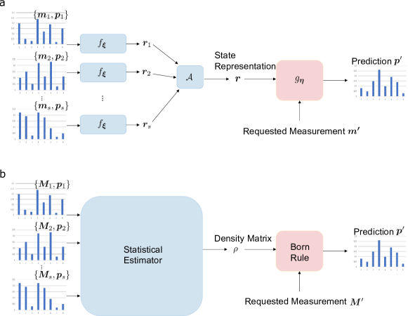
Figure 1: Structure of GQNQ and comparison with quantum state tomography. In GQNQ (a), a representation network receives as input the raw measurement data $\{(\bm{m_{i}},\bm{p}_{i})\}_{i=1}^{s}$ and produces as output $s$ vectors $\bm{r}_{i}=f_{\bm{\xi}}(\bm{m_{i}},\bm{p}_{i})$, that are combined into a single vector $\bm{r}$ by an aggregate function $\cal A$. The vector $\bm{r}$ serves as a concise representation of the quantum state, and is sent to a generation network $g_{\bm{\eta}}$, which predicts the outcome statistics $\bm{p}^{\prime}$ of any desired measurement $\bm{m}^{\prime}$ in the set of measurements of interest. In quantum tomography (b), the raw measurement data are fed into a statistical estimator (such as maximum likelihood), which produces a guess for the density matrix $\rho$. Then, the density matrix is used to predict the outcome probabilities of unperformed quantum measurements via the Born rule. Both GQNQ and quantum tomography use data to infer a representation of the quantum state.

The structure of GQNQ is illustrated in Fig. 1, where we also provide a comparison with quantum state tomography. The first step is to produce a representation of the unknown quantum state $\rho$. In GQNQ, this step is carried out by a representation network, which computes a function $f_{\bm{\xi}}$ depending on parameters $\bm{\xi}$ that are fixed after the training phase (see Methods for details). The representation network receives as input the parametrization of all measurements in $\cal S$ and their outcome statistics on the state $\rho$ that needs to be characterized. For each pair $(\bm{m}_{i},\bm{p}_{i})$, the representation network produces a vector $\bm{r}_{i}=f_{\bm{\xi}}(\bm{m}_{i},\bm{p}_{i})$. The vectors corresponding to different pairs are then combined into a single vector $\bm{r}$ by an aggregate function $\mathcal{A}$. For simplicity, we take the aggregate function to be the average, namely $\bm{r}:=\frac{1}{s}\sum_{i=1}^{s}\bm{r}_{i}$. At this point, the vector $\bm{r}$ is a representation of the quantum state $\rho$.

While tomographic protocols strive to find the density matrix that fits the measurement data, GQNQ is not constrained to a specific choice of state representation. This additional freedom enables the network to construct lower-dimensional representations of quantum states with sufficiently regular structure, such as ground states in well-defined phases of matter, and to make predictions for states that did not appear in the training phase. Notice also that the tomographic reconstruction of the density matrix using statistical estimators, such as maximum likelihood and maximum entropy Teo et al. (2011), is generally more time-consuming than the evaluation of the function $f_{\bm{\xi}}$, due to the computational complexity of the estimation procedure.

Once a state representation has been produced, the next step is to predict the outcome statistics for a new quantum measurement on the state $\rho$. In quantum tomography, the prediction is generated by applying the Born rule on the estimated density matrix. In GQNQ, the task is achieved by a generation network Eslami et al. (2018), which computes a function $g_{\bm{\eta}}$ depending on some parameters $\bm{\eta}$ that are fixed after the training phase. The network receives as input the state representation $\bm{r}$ and the parametrization $\bm{m}^{\prime}$ of the desired measurement $\bm{M}^{\prime}\in\mathcal{M}\setminus\mathcal{S}$, and produces as output a vector $\bm{p}^{\prime}=g_{\bm{\eta}}(\bm{r},\bm{m}^{\prime})$ that approximates the outcome statistics of the measurement $\bm{M}^{\prime}$ on the state $\rho$.

Another difference with quantum tomography is that GQNQ does not require a specific representation of quantum measurements in terms of POVM operators. Instead, a measurement parametrization is sufficient for GQNQ to make its predictions, and the parametrization can even be provided in an encrypted form. Since GQNQ does not require the description of the devices to be provided in clear, it can be used to perform data analysis on a public server, without revealing properties of the quantum hardware, such as the dimension of the underlying quantum system.

So far, we described the GQNQ procedure for learning a single quantum state $\rho$. In the case of multiple states, the same procedure is repeated on each state, every time choosing a (generally different) set of measurements $\mathcal{S}$. Crucially, the network does not need any parametrization of the quantum states, neither it needs the states to be sorted into different classes. For example, if the states correspond to different phases of matter, GQNQ does not need to be told which state belongs to which phase. This feature will be important for the applications to state clustering and classification illustrated later in this paper.

The internal structure of the representation and generation networks is discussed in Supplementary Note VI. The parameters $\bm{\xi}$ and $\bm{\eta}$ are determined in the training phase, in which GQNQ is provided with pairs $(\bm{m},\bm{p})$ consisting of the measurement parametrization/measurement statistics for a fiducial set of measurements ${\cal M}_{*}\subseteq\cal M$, performed on a fiducial set of quantum states $\cal Q_{*}$. In the numerical experiments provided in the Results section, we choose ${\cal M}_{*}=\cal M$, that is, we provide the network with the statistics of all the measurement in $\cal M$. In the typical scenario, the fiducial states and measurements are known, and the training can be done offline, using computer simulated data rather than actual experimental data.

We stress that the parameters $\bm{\xi}$ and $\bm{\eta}$ depend only on the fiducial sets $\cal M_{*}$ and $\cal Q_{*}$ and on the corresponding measurement data, but do not depend on the unknown quantum states that will be characterized later, nor on the subsets of measurements that will be performed on these states. Hence, the network does not need to be re-trained when it is used to characterize a new quantum state $\rho$, nor to be re-trained when one changes the subset of performed measurements $\cal S$.

Summarizing, the main structural features of GQNQ are

• Offline, multi-purpose training: training can be done offline using computer generated data. Once the training has been concluded, the network can be used to characterize and compare multiple states.

• Measurement flexibility: after the training has been completed, the experimenter can freely choose which subset of measurements $\cal S\subset\cal M$ is performed on the unknown quantum states.

• Learner-blindness: the parametrization of the measurements can be provided in an encrypted form. No parametrization of the states is needed.

Later in the paper, we will show that GQNQ can be adapted to an online version of the state learning task Aaronson et al. (2019), thus achieving the additional feature of

• Online prediction: predictions can be updated as new measurement data become available.

Quantum state learning in spin systems. A natural test bed for our neural network model is provided by quantum spin systems Schollwöck et al. (2008); Samaj (2013). In the following, we consider ground states of the one-dimensional transverse-field Ising model and of the XXZ model, both of which are significant for many-body quantum simulations Friedenauer et al. (2008); Kim et al. (2010); Islam et al. (2011). These two models correspond to the Hamiltonians

$$H=-\left(\sum_{i=0}^{L-2}J_{i}\sigma_{i}^{z}\sigma_{i+1}^{z}+\sum_{j=0}^{L-1}\sigma_{j}^{x}\right),$$ (1)

and

$$H=-\left[\sum_{i=0}^{L-2}\Delta_{i}(\sigma_{i}^{x}\sigma_{i+1}^{x}+\sigma_{i}^{y}\sigma_{i+1}^{y})+\sigma_{i}^{z}\sigma_{i+1}^{z}\right]\,,$$ (2)

respectively. In the Ising Hamiltonian (1), positive (negative) coupling parameters $J_{i}$ correspond to ferromagnetic (antiferromagnetic) interactions. For the XXZ Hamiltonian (2), the ferromagnetic phase corresponds to coupling parameters $\Delta_{i}$ in the interval $(-1,1)$. If instead the coupling parameters fall in the region $(-\infty,-1)\cup(1,\infty)$, the Hamiltonian is said to be in the XY phase Yang and Yang (1966).

We start by considering a system of six qubits as example. For the ground states of the Ising model (1), we choose each coupling parameter $J_{i}$ at random following a Gaussian distribution with standard deviation $\sigma=0.1$ and mean $J$. For $J>0$ ($J<0$), this random procedure has a bias towards ferromagnetic (antiferromagnetic) interactions. For $J=0$, ferromagnetic and antiferromagnetic interactions are equally likely. Similarly, for the ground states of the XXZ model (2), we choose each parameter $\Delta_{i}$ at random following a Gaussian distribution with standard deviation $0.1$ and mean value $\Delta$. When $\Delta$ is in the interval $(-1,1)$ ($(-\infty,-1)\cup(1,\infty)$), this random procedure has a bias towards interactions of the ferromagnetic (XY) type.

In addition to the above ground states, we also consider locally rotated GHZ states, of the form $\otimes_{i=1}^{6}U_{i}\ket{\text{GHZ}}$ with $\ket{\text{GHZ}}=\frac{1}{\sqrt{2}}(\ket{000000}+\ket{111111})$ and locally rotated W states, of the form $\otimes_{i=1}^{6}U_{i}\ket{\text{W}}$ with $\ket{\text{W}}=\frac{1}{\sqrt{6}}(\ket{100000}+\dots+\ket{000001})$, where $(U_{i})_{i=1}^{6}$ are unitary matrices of the form $U_{i}=\exp[-\text{i}\theta_{i,z}\sigma_{i,z}]\exp[-\text{i}\theta_{i,y}\sigma_{i,y}]\exp[-\text{i}\theta_{i,x}\sigma_{i,x}],$ where the angles $\theta_{i,x},\theta_{i,y},\theta_{i,z}\in[0,\pi/10]$ are chosen independently and uniformly at random for every $i$.

For the set of all possible measurements $\cal M$, we chose the 729 six-qubit measurements consisting of local Pauli measurements on each qubit. To parameterize the measurements in $\cal M$, we provide the entries in the corresponding Pauli matrix at each qubit, arranging the entries in a 48-dimensional real vector. The dimension of state representation $\bm{r}$ is set to be $32$, which is half of the Hilbert space dimension. In Supplementary Note VII we discuss how the choice of dimension of $\bm{r}$ and the other parameters of the network affect the performance of GQNQ.

GQNQ is trained using measurement data from measurements in $\cal M$ on states of the above four types (see Methods for a discussion of the data generation techniques). We consider both the scenarios where all training data come from states of the same type, and where states of different types are used. In the latter case, we do not provide the network with any label of the state type. After training, we test GQNQ on states of the four types described above. To evaluate the performance of the network, we compute the classical fidelities between the predicted probability distributions and the correct distributions computed from the true states and measurements. For each test state, the classical fidelity is averaged over all possible measurements in $\mathcal{M}\setminus\mathcal{S}$, where $\mathcal{S}$ is a random subset of $30$ Pauli measurements. Then, we average the fidelity over all possible test states.

The results are summarized in Table 1. Each row shows the performances of one particular trained GQNQ when tested using the measurement data from (i) $150$ ground states of Ising model with $J\in\{0.1,\dots,1.5\}$, (ii) $150$ ground states of Ising model with $J\in\{-1.5,-1.4,\dots,-0.1\}$, where $10$ test states are generated per value of $J$, (iii) $10$ ground states of Ising model with $J=0$, (iv) $190$ ground states of XXZ model with $\Delta\in\{-0.9,-0.8,\dots,0.9\}$, (v) $100$ ground states of XXZ model with $\Delta\in\{-1.5,-1.4,\dots,-1.1\}\cup\{1.1,1.2,\dots,1.5\}$, where $10$ test states are generated per value of $\Delta$, (vi) all the states from (i) to (v), (vii) $200$ locally rotated GHZ states (viii) $200$ locally rotated W states (vii), (ix) all the states from (i) to (v), together with (vii) and (viii). In the second column, the input data given to GQNQ is the true probability distribution computed with the Born rule, while in the third and fourth columns, the input data given to GQNQ during test is the finite statistics obtained by sampling the true outcome probability distribution $50$ times and $10$ times, respectively.

Table 1: Average classical fidelities between the predictions of GQNQs and the ground truths with respect to different types of six-qubit states.

Types of states for training and test	noiseless	$50$ shots	$10$ shots
(i) Ising ground states with ferromagnetic bias	0.9870	0.9869	0.9862
(ii) Ising ground states with antiferromagnetic bias	0.9869	0.9867	0.9849
(iii) Ising ground states with no bias	0.9895	0.9894	0.9894
(iv) XXZ ground states with ferromagnetic bias	0.9809	0.9802	0.9787
(v) XXZ ground states with XY phase bias	0.9601	0.9548	0.9516
(vi) (i)-(v) together	0.9567	0.9547	0.9429
(vii) GHZ state with local rotations	0.9744	0.9744	0.9742
(viii) W state with local rotations	0.9828	0.9826	0.9821
(ix) (i)-(v), (vii) and (viii) together	0.9561	0.9543	0.9402

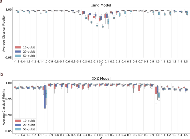
Figure 2: Performances of GQNQs on Ising model ground states and XXZ model ground states visualized by boxplots Williamson et al. (1989). Figure (a) shows the average classical fidelities of predictions given by three GQNQs for ten-, twenty- and fifty-qubit ground states of Ising model (1), respectively, with respect to different values of $J\in\{-1.5,-1.4,\dots,1.5\}$. Figure (b) shows the performances of another three GQNQs for ten-, twenty- or fifty-qubit ground states of XXZ model (2), respectively, with respect to different values of $\Delta\in\{-1.5,-1.4,\dots,1.5\}$. Given outcome probability distributions for all $\bm{m}\in\mathcal{S}$, each box shows the average classical fidelities of predicted outcome probabilities, averaged over all measurements in $\mathcal{M}\setminus\mathcal{S}$, for ten instances.

The results shown in Table 1 indicate that the performance with finite statistics is only slightly lower than the performance in the ideal case. It is also worth noting that GQNQ maintains a high fidelity even when used on multiple types of states.

Recall that the results in Table 1 refer to the scenario where GQNQ is trained with the full set of six-qubit Pauli measurements, which is informationally complete. An interesting question is whether the learning performance would still be good if the training used a non-informationally complete set of measurements. In Supplementary Note IX, we show that fairly accurate predictions can be made even if $\cal M$ consists only of $72$ randomly chosen Pauli measurements.

While GQNQ makes accurate predictions for state families with sufficient structure, it should not be expected to work universally well on all possible quantum states. In Supplementary Note VIII, we considered the case where the network is trained and tested on arbitrary six-qubit states, finding that the performance of GQNQ drops drastically. In Supplementary Note X, we also provide numerical experiments on the scenario where some types of states are overrepresented in the training phase, potentially causing overfitting when GQNQ is used to characterize unknown states of an underrepresented type.

We now consider multiqubit states with $10$, $20$, and $50$ qubits, choosing the measurement set $\cal M$ to consist of all two-qubit Pauli measurements on nearest-neighbor qubits and $\mathcal{S}$ a subset containing $s=30$ measurements randomly chosen from $\mathcal{M}$. Here the dimension of state representation $\bm{r}$ is chosen to be $24$, which guarantees a good performance in our numerical experiments.

For the Ising model, we choose the coupling between each nearest-neighbour pair of spins to be either consistently ferromagnetic for $J\geq 0$ or consistently antiferromagnetic for $J<0$: for $J\geq 0$ we replace each coupling $J_{i}$ in Eq. (1) by $|J_{i}|$, and for $J<0$ we replace $J_{i}$ by $-|J_{i}|$. The results are illustrated in Fig. 2. The figure shows that the average classical fidelities in both ferromagnetic and antiferromagnetic regions are close to one, with small drops around the phase transition point $J=0$. The case where both ferromagnetic and anti-ferromagnetic interactions are present is studied in Supplementary Note XI, where we observe that the learning performance is less satisfactory in this scenario.

For XXZ model, the average classical fidelities in the XY phase are lower than those in the ferromagnetic interaction region, which is reasonable due to higher quantum fluctuations in the XY phase Samaj (2013). At the phase transition points $\Delta=\pm 1$, the average classical fidelities drop more significantly, partly because the abrupt changes of ground state properties at the critical points make the quantum state less predictable, and partly because the states at phase transition points are less represented in the training data set.

Quantum state learning on a harmonic oscillator. We now test GQNQ on states encoded in harmonic oscillators, i.e. continuous-variable quantum states, including single-mode Gaussian states, as well as non-Gaussian states such as cat states and GKP states Gottesman et al. (2001), both of which are important for fault-tolerant quantum computing Gottesman et al. (2001); Albert et al. (2018). For the measurement set $\cal M$, we choose $300$ homodyne measurements, that is, $300$ projective measurements associated to quadrature operators of the form $(e^{i\theta}\,\hat{a}^{\dagger}+e^{-i\theta}\,\hat{a})/2$, where $\hat{a}^{\dagger}$ and $\hat{a}$ are bosonic creation and annihilation operators, respectively, and $\theta$ is a uniformly distributed phase in the interval $[0,\pi)$. For the subset $\cal S$, we pick $10$ random quadratures. For the parametization of the measurements, we simply choose the corresponding phase $\theta$. Since the homodyne measurements have an unbounded and continuous set of outcomes, here we truncate the outcomes into a finite interval (specifically, at $\pm 6$) and discretize them, dividing the interval into $100$ bins of equal width. The dimension of the representation vector $\bm{r}$ is chosen to be $16$.

Table 2: Performances of GQNQ on continuous-variable quantum states.

Type of states for training and test	i. noiseless	worst case for i	ii. $\sigma$(noise)$=0.05$	worst case for ii	iii. $\sigma(\theta)=0.05$	worst case for iii
(i) Squeezed thermal states	$0.9973$	$0.9890$	$0.9964$	$0.9870$	$0.9972$	$0.9889$
(ii) Cat states	$0.9827$	$0.9512$	$0.9674$	$0.9053$	$0.9822$	$0.9461$
(iii) GKP states	$0.9762$	$0.9405$	$0.9746$	$0.9359$	$0.9758$	$0.9405$
(iv) (i)-(iii) together	$0.9658$	$0.9077$	$0.9264$	$0.8387$	$0.9643$	$0.9030$

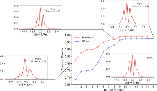
Figure 3: Online learning of cat states in 15 time steps. Each red point shows the classical fidelity, averaged over all the possible measurements in $\cal M$ and over all the cat states in the test set, which we take to be the same as in the experiments in the previous section. Each blue point is the worst-case classical fidelity over all possible query measurements, averaged over all the test states. Real outcome statistics and predicted outcome statistics at quadrature phase $\theta=3/4\pi$ for an example cat state $\ket{2.22+1.41\text{i},\pi/4}_{\text{cat}}$ are plotted.

In Table 2 we illustrate the performance of GQNQ on (i) $200$ squeezed thermal states with thermal variance $V\in[1,2]$ and squeezing parameter $s$ satisfying $|s|\in[0,0.5]$, $\text{arg}(s)\in[0,\pi]$, (ii) $200$ cat states corresponding to superpositions of coherent states with opposite amplitudes $\ket{\alpha,\phi}_{\text{cat}}:=\frac{1}{\sqrt{\mathcal{N}}}(\ket{\alpha}+\text{e}^{\text{i}\phi}\ket{-\alpha})$, where $\mathcal{N}=2(1+\text{e}^{-|\alpha|^{2}}\cos\phi)$, $|\alpha|\in[1,3]$ and $\phi\in\{0,\frac{\pi}{8},\dots,\pi\}$, (iii) $200$ GKP states that are superpositions of displaced squeezed states $\ket{\epsilon,\theta,\phi}_{\text{gkp}}:=\text{e}^{-\epsilon\hat{n}}\left(\cos\theta\ket{0}_{\text{gkp}}+\text{e}^{\text{i}\phi}\sin\theta\ket{1}_{\text{gkp}}\right)$ where $\hat{n}=\hat{a}^{\dagger}\hat{a}$ is the photon number operator, $\epsilon\in[0.05,0.2]$, $\theta\in[0,2\pi)$, $\phi\in[0,\pi]$, and $\ket{0}_{\text{gkp}}$ and $\ket{1}_{\text{gkp}}$ are ideal GKP states, and (iv) all the states from (i), (ii), and (iii).

For each type of states, we provide the network with measurement data from $s=10$ random homodyne measurements, considering both the case where the data is noiseless and the case where it is noisy. The noiseless case is shown in the second and third columns of Table 2, which show the classical fidelity in the average and worst-case scenario, respectively. In the noisy case, we consider both noise due to finite statistics, and noise due to an inexact specification of the measurements in the test set. The effects of finite statistics are modelled by adding Gaussian noise to each of the outcome probabilities of the measurements in the test. The inexact specification of the test measurements is modelled by rotating each quadrature by a random angle $\theta_{i}$, chosen independently for each measurement according to a Gaussian distribution. The fourth and the fifth columns of Table 2 illustrate the effects of finite statistics, showing the classical fidelities in the presence of Gaussian added noise with variance $0.05$. In the sixth and seventh columns, we include the effect of an inexact specification of the homodyne measurements, introducing Gaussian noise with variance $0.05$. In all cases, the classical fidelity of predictions are computed with respect to the ideal noiseless probability distributions.

In Supplementary Note XI we also provide a more detailed comparison between the predictions and the corresponding ground truths in terms of actual probability distributions, instead of their classical fidelities.

Application to online learning. After GQNQ has been trained, it can be used for the task of online quantum state learning Aaronson et al. (2019). In this task, the various pieces of data are provided to the learner at different time steps. At the $i$-th time step, with $i\in\{1,\dots,n\}$, the experimenter performs a measurement $\bm{M}_{i}$, obtaining the outcome statistics $\bm{p}_{i}$. The pair $(\bm{m_{i}},\bm{p_{i}})$ is then provided to the learner, who is asked to predict the measurement outcome probabilities for all measurements in the set $\mathcal{M}\setminus\mathcal{S}_{i}$ with ${\cal S}_{i}:=\{\bm{M}_{j}\}_{j\leq i}$.

Online learning with GQNQ can be achieved with the following procedure. Initially, the state representation vector is set to $\bm{r}(0)=(0,\dots,0)$. At the $i$-th time step, GQNQ computes the vector $\bm{r}_{i}=f_{\bm{\xi}}(\bm{m}_{i},\bm{p}_{i})$ and updates the state representation to $\bm{r}(i)=[(i-1)\,\bm{r}(i-1)+\bm{r}_{i}]/i$. The updated state representation is then fed into the generation network, which produces the required predictions. Note that updating the state representation does not require time-consuming operations, such as a maximum likelihood analysis. It is also worth noting that GQNQ does not need to store all the measurement data received in the past: it only needs to store the state representation $\bm{r}(i)$ from one step to the next.

A numerical experiment on online learning of cat states is provided in Fig. 3. The figure shows the average classical fidelity at 15 subsequent time steps corresponding to 15 different homodyne measurements performed on copies of unknown cat states. The fidelity increases over time, confirming the intuitive expectation that the learning performance should improve when more measurement data are provided.

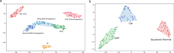
Figure 4: Two-dimensional embeddings of multiqubit and continuous-variable states. Subfigure (a) shows two-dimensional embeddings of state representation vectors produced by GQNQ on Ising model (ferromagnetic and antiferromagnetic) ground states, XXZ model (ferromagnetic and XY phase) ground states, locally rotated GHZ and W states. Subfigure (b) shows two-dimensional embeddings of the state representation vectors of squeezed thermal states, cat states and GKP states. In both subfigures, shaded areas are added to help visualize the various type of states. Note that the representation vectors generated by GQNQ of states of the same type are near to each other in the two-dimensional embeddings.

Application to state clustering and classification. The state representation constructed by GQNQ can also be used to perform tasks other than predicting the outcome statistics of unmeasured POVMs. One such task is state clustering, where the goal is to group the representations of different quantum states into multiple disjoint sets in such a way that quantum states of the same type fall into the same set.

We now show that clusters naturally emerge from the state representations produced by GQNQ. To visualize the clusters, we feed the state representation vectors into a $t$-distributed stochastic neighbor embedding ($t$-SNE) algorithm Van der Maaten and Hinton (2008), which produces a mapping of the representation vectors into a two-dimensional plane, according to their similarities. We performed numerical experiments using the types of six-qubit states in Table 1 and the types of continuous-variable states in Table 2. For simplicity, we restricted the analysis to state representation vectors constructed from noiseless input data.

The results of our experiments are shown in Fig. 4. The figure shows that states with significantly different physical properties correspond to distant points in the two-dimensional embedding, while states with similar properties naturally appear in clusters. For example, the ground states of the ferromagnetic XXZ model and the ground states in the gapless XY phase are clearly separated in Fig. 4(a), in agreement with the fact that there is an abrupt change of quantum properties at the phase transition point. On the other hand, in Fig. 4(a), the ferromagnetic region of the Ising model is next to the antiferromagnetic region, both of which are gapped and short-range correlated. The ferromagnetic region of the Ising model appears to have some overlap with the region of GHZ states with local rotations, in agreement with the fact that the GHZ state is approximately a ground state of the ferromagnetic Ising model in the large $J$ limit.

The visible clusters in the two-dimensional embedding suggest that any unsupervised clustering algorithm could effectively cluster the states according to their representation vectors. To confirm this intuition, we applied a Gaussian mixture model Bishop and Nasrabadi (2006) to the state representation vectors and chose the number of clusters to be equal to the actual number of state types (six for the six-qubit states, and three for the continuous-variable states). The portion of states whose types match the clusters is $94.67\%$ for the six-qubit states, and $100\%$ for the continuous-variable states.

The state representation produced by GQNQ can also be used to predict physical properties in a supervised model where an additional neural network is provided with labelled examples of states with a given property. In this setting, supervision can enable a more refined classification of quantum states, compared to the unsupervised clustering discussed before.

To illustrate the idea, we considered the problem of distinguishing between two different regimes in the Ising model, namely a regime where ferromagnetic interactions dominate ($J>1$), and a regime both ferromagnetic and antiferromagnetic interactions are present ($0<J<1$). For convenience, we refer to these two regimes as to the pure and mixed ferromagnetic regimes, respectively. We use an additional neural network to learn whether a ground state corresponds to a Hamiltonian in the pure ferromagnetic regime or in the mixed one, using the state representation $\bm{r}$ of Ising ground states with ferromagnetic bias obtained from noiseless measurement data. The prediction reaches a success rate of $100\%$, $100\%$ and $99\%$ for ten-qubit, twenty-qubit and fifty-qubit ground states in our test sets, respectively. These high values can be contrasted with the clustering results in Fig. 4, where the pure ferromagnetic regime and the mixed one appear close to each other in the two-dimensional embedding.

III Discussion

Table 3: Performances of GQNQ on cat states as an unsupervised learner

state	$s=50$ (Avg)	$s=50$ (Worst)	$s=10$ (Avg)	$s=10$ (Worst)
$\ket{2,0}_{\text{cat}}$	$0.9918$	$0.9614$	$0.9912$	$0.9610$
$\ket{2,\pi/4}_{\text{cat}}$	$0.9917$	$0.9602$	$0.9745$	$0.9236$
$\ket{2.22+1.41\text{i},\pi/4}_{\text{cat}}$	$0.9779$	$0.9171$	$0.9671$	$0.9133$

Many works have explored the use of generative models for quantum state characterization Torlai et al. (2018); Torlai and Melko (2018); Carrasquilla et al. (2019); Tiunov et al. (2020); Ahmed et al. (2021a), and an approach based on representation learning was recently proposed by Iten et al Iten et al. (2020). The key difference between GQNQ and previous approaches concerns the training phase. In most previous works, the neural network is trained to reconstruct a single quantum state from experimental data. While this procedure can in principle be applied to learn any state, the training is state-specific, and the information learnt by the network through training on a given state cannot be automatically transferred to the reconstruction of a different quantum state, even if that state is of the same type. In contrast, the training of GQNQ works for multiple quantum states and for states of multiple types, thus enabling a variety of tasks, such as quantum state clustering and classification.

Another difference with previous works is that the training phase for GQNQ can use classically simulated data, rather than actual experimental data. In other words, the training can be carried out in an offline mode, before the quantum states that need to be characterized become available. By moving the training to offline mode, GQNQ can be significantly faster than other data-driven approaches that need to be trained with experimental data from unknown quantum states. The flip side of this advantage, however, is that offline training requires a partial supervision, which is not required in other state reconstruction approaches  Torlai et al. (2018); Torlai and Melko (2018); Carrasquilla et al. (2019). Indeed, the training of GQNQ requires quantum states in the same family as the tested state, and in order to implement the training offline one needs a good guess for the type of quantum state that will need to be characterized.

The situation is different if the training is done online, with actual experimental data provided from the quantum state to be characterized. In this setting, GQNQ behaves as a completely unsupervised learner that predicts the outcome statistics of unperformed measurements using measurement data obtained solely from the quantum state under consideration. Note that in this case the set of fiducial measurements $\mathcal{M}_{*}$ coincides with the set of performed measurements ${\cal S}\subset\cal M$. The details of the training procedure are provided in Supplementary Note XII. We performed numerical experiments in which GQNQ was trained with data from a single cat state, using data from $10$ or $50$ homodyne measurements. After the training, GQNQ was asked to predict the outcome statistics of a new randomly chosen homodyne measurement. The results are summarized in Table 3, where we show both the average classical fidelities averaged over all query measurements and worst-case classical fidelities over all query measurements.

Finally, we point out that our learning model shares some conceptual similarity with Aaronson’s “pretty good tomography” Aaronson (2007), which aims at producing a hypothesis state that accurately predicts the outcome probabilities of measurements in a given set. While in pretty good tomography the hypothesis state is a density matrix, the form of the state representation in GQNQ is determined by the network itself. The flexibility in the choice of state representation allows GQNQ to find more compact descriptions for sufficiently regular sets of states. On the other hand, pretty good tomography is in principle guaranteed to work accurately for arbitrary quantum states, whereas the performance of GQNQ can be more or less accurate depending on the set of states, as indicated by our numerical experiments. An important direction of future research is to find criteria to determine a priori which quantum state families can be learnt effectively by GQNQ. This problem is expected to be challenging, as similar criteria are still lacking even in the original application of generative query networks to classical image processing.

IV Methods

Data generation procedures. Here we discuss the training/test dataset generation procedures. In the numerical experiments for ground states of Ising models and XXZ models, the training set is composed of $40$ different states for each value of $J$ and $\Delta$, while the test set is composed of $10$ different states for each value of $J$ and $\Delta$. For GHZ and W states with local rotations, we generate $800$ states for training and $200$ states for testing.

In the continuous-variable experiments, we randomly generate $10000$ different states for each of the three families of squeezed thermal states, cat states, and GKP states. We then split the generated states into a training set and testing set, with a ratio of $4:1$.

In the testing stage, the noiseless probability distributions for one-dimensional Ising models and XXZ models are generated by solving the ground state problem, either exactly (in the six qubit case) or approximately by density-matrix renormalization group (DMRG) algorithm Schollwöck (2005) (for $10$, $20$ and $50$ qubits). The data of continuous-variable quantum states are generated by simulation tools provided by Strawberry Fields Killoran et al. (2019).

Network training. The training data set of GQNQ includes measurement data from $N$ quantum states, divided into $N/B$ batches of $B$ states each. For each state in a batch, a subset of measurements $\mathcal{M}_{1}\subset\mathcal{M}$ is randomly picked, and the network is provided with all the pairs $(\bm{m},\bm{p})$, where $\bm{m}$ is the parametrization of a measurement in ${\cal M}_{1}$ and $\bm{p}$ is the corresponding vector of outcome probabilities on the state under consideration. The network is then asked to make predictions on the outcome probabilities of the rest of the measurements in $\mathcal{M}\setminus\mathcal{M}_{1}$, and the loss is computed from the difference between the real outcome probabilities (computed with the Born rule) and the model’s predictions (see Supplementary Note VI for the specific expression of the loss function). For each batch, we optimize the parameters $\bm{\xi}$ and $\bm{\eta}$ of GQNQ by updating them along the opposite direction of the gradient of the loss function with respect to $\bm{\xi}$ and $\bm{\eta}$, using Adam optimizer Kingma and Ba (2014) and batch gradient descent. The pseudocode for the training algorithm is also provided in Supplementary Note VI.

The training is repeated for $E$ epochs. In each epoch of the training phase, we iterate the above procedure over the $N/B$ batches of training data. For the numerical experiments in this paper, we typically choose $B=30$ and $E=200$.

Network testing. After training, the parameters of GQNQ are fixed, and the performance is then tested with these fixed parameter values. For each test state, we randomly select a subset $\mathcal{S}$ from the set $\mathcal{M}$ of POVM measurements, input the associated measurement data to the trained network, and ask it to predict the outcome probabilities for all the measurements in $\mathcal{M}\setminus\mathcal{S}$. Then we calculate the classical fidelity between each output prediction and the corresponding ground truth.

Hardware. Our neural networks are implemented by the pytorch Paszke et al. (2019) framework and trained on four NVIDIA GeForce GTX 1080 Ti GPUs.

V acknowledgement

This work was supported by funding from the Hong Kong Research Grant Council through grants no. 17300918 and no. 17307520, through the Senior Research Fellowship Scheme SRFS2021-7S02, the Croucher Foundation, and by the John Templeton Foundation through grant 61466, The Quantum Information Structure of Spacetime (qiss.fr). YXW acknowledges funding from the National Natural Science Foundation of China through grants no. 61872318. Research at the Perimeter Institute is supported by the Government of Canada through the Department of Innovation, Science and Economic Development Canada and by the Province of Ontario through the Ministry of Research, Innovation and Science. The opinions expressed in this publication are those of the authors and do not necessarily reflect the views of the John Templeton Foundation.

SUPPLEMENTARY NOTES

VI Implementation details of GQNQ

VI.1 Structure of GQNQ

As shown in Fig. 5, our proposed Generative Query Network for quantum state learning (GQNQ) is mainly composed of a representation network $f_{\bm{\xi}}$, an aggregate function $\mathcal{A}$ and a generation network $g_{\bm{\eta}}$.

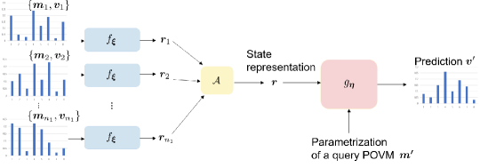
Figure 5: Structure of GQNQ.

The representation network $f_{\bm{\xi}}$ consists of multiple dense layers Aggarwal et al. (2018), also called full-connected layers and we depict its structure in Fig. 6. $\bm{\xi}$ contains trainable parameters of all layers. The input of the representation network is a pair $(\bm{m}_{i},\bm{p}_{i})$, where $\bm{m}_{i}$ is parameterization of a POVM measurement and $\bm{p}_{i}$ is its corresponding measurement outcome probabilities. The output $\bm{r}_{i}$ can be regarded as an abstract representation of $(\bm{m}_{i},\bm{p}_{i})$. Here, for simplicity, we just use the average function $\bm{r}:=\frac{1}{s}\sum_{i=1}^{s}\bm{r}_{i}$ as the aggregate function but we believe other more sophisticated architecture such as recurrent neural network Aggarwal et al. (2018) may achieve better performance, although it will lead to higher requirements for hardware and hyperparameter tuning.

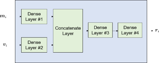
Figure 6: Structure of the representation network.

The generation network $g_{\bm{\eta}}$ is special because its structure is different in the training and test phase. Here $\bm{\eta}$ contains all trainable parameters in the generation network. In the test phase, the generation network consists of two dense layers and one long short-term memory (LSTM) cell Hochreiter and Schmidhuber (1997), and we depict its structure in Fig. 7. The input of this generation network is the state representation $\bm{r}$ and the parameterization $\bm{m}^{\prime}$ of a query POVM measurement and the output $\mathcal{N}^{\prime}$ is a distribution of the prediction $\bm{p}^{\prime}$ of measurement outcome probabilities corresponding to $\bm{m}^{\prime}$. $\bm{h}_{0}$, $\bm{c}_{0}$ and $\bm{u}_{0}$ are some internal parameters, all of which are initialized as zero tensors. As we can see, the generation network execute Dense Layer #1 and the LSTM cell for $L$ times while $\bm{m}^{\prime}$ and $\bm{r}$ are injected to the network for each time. It is worth mentioning that $\bm{z}_{i}$ ($i\in\mathbb{N},i<L$) can be viewed as a hidden variable that obeys a prior Gaussian distribution $\mathcal{N}_{i}$ generated by Dense Layer #1 from $\bm{h}_{i}$. In the end, the output $\bm{u}_{L}$ of the last LSTM cell is fed into a second dense layer (Dense Layer #2) to obtain the output $\mathcal{N}^{\prime}$, from which the prediction $\bm{p}^{\prime}$ is sampled. In Fig. 8, we depict the generation network exploited in the training. Here, an extra input $\bm{p}^{\prime}_{true}$ is available because we know the real outcome probabilities in the training phase. Furthermore, we utilize another LSTM cell and another dense layer (Dense Layer #3) to generate a posterior distribution $\mathcal{N}_{i}^{2}$ from $\bm{p}^{\prime}_{true}$ of the hidden variable $\bm{z}_{i}$ rather than sampling $\bm{z}_{i}$ from a prior distribution $\mathcal{N}_{i}^{1}$. The advantage of such design is that we can make good use of the information of $\bm{p}^{\prime}_{true}$ to obtain better $\bm{z}_{i}$ during the generation. $\bm{h}_{0}^{1}$, $\bm{c}_{0}^{1}$, $\bm{h}_{0}^{2}$, $\bm{c}_{0}^{2}$ and $\bm{u}_{0}$ are some internal parameters, all of which are initialized as zero tensors.

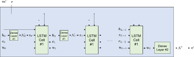
Figure 7: Structure of the generation network in the test.

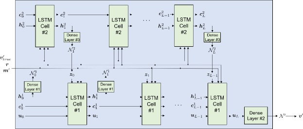
Figure 8: Structure of the generation network in the training.

VI.2 Training of GQNQ

We define the loss function $\mathcal{L}$ of the training in Eq. (3).

$$\mathcal{L}(\bm{\xi},\bm{\eta})=\mathop{\mathbb{E}}[-\ln\mathcal{N}^{\prime}(\bm{p}^{\prime}_{true})+\sum_{j=0}^{L-1}{\rm KL}(\mathcal{N}_{j}^{1},\mathcal{N}_{j+1}^{2})],$$ (3)

where $\mathcal{N}^{\prime}(\bm{p}^{\prime}_{true})$ denotes the relative likelihood that the variable following distribution $\mathcal{N}^{\prime}$ takes the value of $\bm{p}^{\prime}_{true}$ and ${\rm KL}$ represents KL divergence Kullback (1997) of two Gaussian distributions. The first term of this loss function can be interpreted as the reconstruction loss, which can guide the model to acquire more accurate predictions. The second term is a regularization term utilized for seeking a better prior distribution of the hidden variable $\bm{z}_{i}$ in the generation process, which is constructive to improving the accuracy of the predictions further.

We adopt batch gradient descent Ruder (2016) and the Adam optimizer Kingma and Ba (2014) to minimize this loss function in the training. The batch size is set to $10$ or $20$ in all of our experiments and the learning rate decreases gradually with the increase of the number of training epochs.

Our neural networks are implemented by the pytorch Paszke et al. (2019) framework and trained on four NVIDIA GeForce GTX 1080 Ti GPUs. The training time is less than three hours for each task discussed in this paper. The ground states of the Hamiltonian of one-dimensional Ising models utilized in our numerical experiments are solved by the exact method for the scenario of $L=6$ and are approximately solved by density-matrix renormalization group (DMRG) Schollwöck (2005) for the scenario of $L=10$, $20$ and $50$. The data of continuous-variable quantum states are generated by simulation tools provided in Strawberry Fields Killoran et al. (2019).

We present the whole training procedure by pseudocode in Algorithm 1 following the notations introduced in main text.

Data: number of states in training set $N$, state measurement results $\{\{(\bm{m}_{i},\bm{p}^{k}_{i})\}_{i=1}^{n}\}_{k=1}^{N}$, maximum number of known POVM measurement results for each state $a$, maximum number of epochs $E$, learning rate $\delta$, batch size $B$.

Initialize parameters $\bm{\xi}$ and $\bm{\eta}$ randomly, $e=0$;

while $e<E$ do

       $\mathcal{L}=0$;

       for $k=1$ to $N$ do

             Generate a random integer number $n_{1}$ from $[1,a]$;

             Randomly select $n_{1}$ pairs of $(\bm{m}_{i},\bm{p}_{i}^{k})$ from $\{(\bm{m}_{i},\bm{p}^{k}_{i})\}_{i=1}^{n}$ and denote them as $\{(\bm{m}_{i_{j}},\bm{p}^{k}_{i_{j}})\}_{j=1}^{n_{1}}$, where $\{i_{j}\}_{j=1}^{n}$ is a permutation of $\{1,\dots,n\}$ ;

             Input each of $\{(\bm{m}_{i_{j}},\bm{p}^{k}_{i_{j}})\}_{j=1}^{n_{1}}$ into the representation network $f_{\bm{\xi}}$ to obtain the representations $\{\bm{r}_{i_{j}}\}_{j=1}^{n_{1}}$ as $\bm{r}_{i_{j}}=f_{\bm{\xi}}(\bm{m}_{i_{j}},\bm{p}^{k}_{i_{j}})$ ;

             Calculate the state representation by an aggregate function $\mathcal{A}$ as $\bm{r}=\mathcal{A}(\{\bm{r}_{i_{j}}\}_{j=1}^{n_{1}})$ ;

             Input $\bm{r}$ and the remaining $\{\bm{m}_{i_{j}}\}_{j=n_{1}+1}^{n}$ into the generation network $g_{\bm{\eta}}$ to obtain the predictions $\{\bm{p}^{\prime k}_{i_{j}}\}_{j=n_{1}+1}^{n}$ of measurement outcome distributions as $\bm{p}^{\prime k}_{i_{j}}=g_{\bm{\eta}}(\bm{r},\bm{m}_{i_{j}})$;

             Calculate the loss $l$ with Eq. (3) by comparing $\{\bm{p}^{\prime k}_{i_{j}}\}_{j=n_{1}+1}^{n}$ with $\{\bm{p}^{k}_{i_{j}}\}_{j=n_{1}+1}^{n}$ and update $\mathcal{L}$ as $\mathcal{L}=\mathcal{L}+l$ ;

             if $k\ \text{mod}\ B=0$ then

                   Calculate $\nabla_{\bm{\xi}}\mathcal{L}$ and $\nabla_{\bm{\eta}}\mathcal{L}$ ;

                   Update $\bm{\xi}$ and $\bm{\eta}$ as $\bm{\xi}=\bm{\xi}-\delta\nabla_{\bm{\xi}}\mathcal{L}$, $\bm{\eta}=\bm{\eta}-\delta\nabla_{\bm{\eta}}\mathcal{L}$ ;

                   $\mathcal{L}=0$;

                  

            

      $e=e+1$ ;

      

Algorithm 1 Training of generative query network for quantum state learning.

VI.3 Details of Experiments

Datasets.

In the experiments for ground states of Ising models and XXZ models, the training set is composed of $40$ different states for each $J$ or $\Delta$ while the test set is composed of $10$ different states for each $J$ or $\Delta$. As for the experiments for GHZ state with local rotation and W state with local rotation, we generate $800$ states for training and $200$ states for test. In the experiments for continuous-variable quantum states, we randomly generate $10000$ different cat states, gaussian states and GKP states and split them into training and test sets with $4:1$ ratio.

Number of trainable parameters.

We mainly adopt three kinds of models for three different tasks. In the experiments for learning discrete quantum states, we exploit the models with $6676544$ trainable parameters for the scenario of $L=6$ while exploiting the models with $45484$ trainable parameters for the scenario of $L=10,20$ and $50$. In the experiments for learning continuous-variable quantum states, we exploit the models with $35572$ trainable parameters.

Maximum number of known POVM measurement results for each state in the training.

We set maximum number of known POVM measurement results for each state $a$ in the training as $200$ for the six-qubit cases, $50$ for the $10$-, $20$- and $50$-qubit cases and $150$ for the cases of continuous states.

Initialization and learning rate.

For each task, we initialize the parameters of the models randomly before the training. The learning rate is set as $0.01$ initially and decreases as the number of iterations increases.

Number of epochs and training time.

We usually set the maximum number of epochs $E$ as $200$ and the batch size $B$ as $30$ in the training. The training time varies with the size of training set for each task while the training time is always less than three hours in all of the experiments.

VII Hyperparameters

As introduced above, there are some hyperparameters in our GQNQ model and the most significant ones are the dimensions of $\bm{r}_{i}$, $\bm{h}_{i}$ and $\bm{z}_{i}$, because they affect the size of the state representation and the complexity of the model, and thus affect the performance of the model. We denote them as $d_{\bm{r}}$, $d_{\bm{h}}$ and $d_{\bm{z}}$ respectively. In this section, we conduct a series of experiments to explore how the choice of hyperparameters affects the performance of the proposed model. We take the settings of learning $6$-qubit states introduced in the main text as examples. In each experiment, different settings of hyperparameters are adopted and the results are shown in Table 4.

We can easily find that as the complexity of the model increases, the performance of the model becomes better. However, it must be pointed out that the complexity of the model cannot be arbitrarily high considering the memory size and the difficulty of training, and the models with $d_{\bm{r}}=32$, $d_{\bm{h}}=96$ and $d_{\bm{z}}=32$ are the most complicated ones we consider in this paper.

Table 4: Average classical fidelity between predicted outcome statistics and real outcome statistics, averaged over all the test states and random query measurements. The eight rows correspond to eight different scenarios, where GQNQ is trained and tested over measurement data of nine sets of states. The values of $d_{\bm{r}}$, $d_{\bm{h}}$ and $d_{\bm{z}}$ are different for each column.

Types of states	$d_{\bm{r}}=2$, $d_{\bm{h}}=2$, $d_{\bm{z}}=2$	$d_{\bm{r}}=2$, $d_{\bm{h}}=6$, $d_{\bm{z}}=2$	$d_{\bm{r}}=4$, $d_{\bm{h}}=12$, $d_{\bm{z}}=4$	$d_{\bm{r}}=8$, $d_{\bm{h}}=24$, $d_{\bm{z}}=8$	$d_{\bm{r}}=16$, $d_{\bm{h}}=48$, $d_{\bm{z}}=16$	$d_{\bm{r}}=32$, $d_{\bm{h}}=96$, $d_{\bm{z}}=32$
(i) Ising ground states with ferromagnetic bias	0.7987	0.8835	0.8981	0.9255	0.9543	0.9870
(ii) Ising ground states with antiferromagnetic bias	0.7896	0.8739	0.8894	0.9236	0.9562	0.9869
(iii) Ising ground states with no bias	0.7999	0.8911	0.8993	0.9277	0.9596	0.9895
(iv) XXZ ground states with ferromagnetic bias	0.6386	0.7683	0.9038	0.9546	0.9603	0.9809
(v) XXZ ground states with XY phase bias	0.7515	0.8102	0.8359	0.8924	0.9352	0.9601
(vi) (i)-(v) together	0.7143	0.7709	0.8376	0.8739	0.9178	0.9567
(vii) GHZ state with local rotations	0.8342	0.8816	0.9271	0.9502	0.9579	0.9744
(viii) W state with local rotations	0.9249	0.9310	0.9579	0.9733	0.9771	0.9828
(ix) (i)-(v), (vii) and (viii) together	0.6936	0.7685	0.8369	0.8725	0.9085	0.9561

VIII Arbitrary State Learning

Furthermore, we conducted experiments to learn arbitrary $6$-qubit quantum states and the results are shown in Table 5. We claim that all models failed in this case, since we find that they always yield distributions close to the uniform distribution for any query measurement, which means that the model cannot learn an effective state representation to generate accurate measurement outcome statistics. A possible explanation is that the model is not complicated enough to handle an unstructured, highly complex dataset. Although a more complicated model might be more effective intuitively, such a model may require larger training set and be less efficient. As expected, our GQNQ model is designed for quantum states sharing a common structure and is not suitable for arbitrary quantum states.

Table 5: Average classical fidelity between predicted outcome statistics and real outcome statistics for the arbitrary states, averaged over all the test states and random query measurements. The values of $d_{\bm{r}}$, $d_{\bm{h}}$ and $d_{\bm{z}}$ are different for each column.

Types of states	Uniform distribution	$d_{\bm{r}}=2$, $d_{\bm{h}}=2$, $d_{\bm{z}}=2$	$d_{\bm{r}}=2$, $d_{\bm{h}}=6$, $d_{\bm{z}}=2$	$d_{\bm{r}}=4$, $d_{\bm{h}}=12$, $d_{\bm{z}}=4$	$d_{\bm{r}}=8$, $d_{\bm{h}}=24$, $d_{\bm{z}}=8$	$d_{\bm{r}}=16$, $d_{\bm{h}}=48$, $d_{\bm{z}}=16$	$d_{\bm{r}}=32$, $d_{\bm{h}}=96$, $d_{\bm{z}}=32$
Arbitrary 6-qubit state	0.8879	0.8879	0.8879	0.8879	0.8879	0.8879	0.8879

IX Generalization from Informationally Incomplete Measurements

In this section, we will further discuss the generalization performance of our proposed model in the examples of six-qubit quantum states. We mainly focus on how the information completeness of the measurement class affects the final performance. Rather than setting the class of measurements $\mathcal{M}$ as the set of all $729$ six-qubit Pauli-basis measurements, we construct $\mathcal{M}$ by randomly selecting $72$ different six-qubit Pauli-basis measurements in each experiment here. For each dataset we discussed, we did such experiments and averaged the results. The results are shown in Table 6.

As the experimental results show, our proposed model still has a satisfactory performance when the measurement class is not informationally complete. Meanwhile, we also find that the model will generalize worse as the complexity of datasets increases. A possible explanation is that more information is needed to yield accurate state representations when the dataset is composed of multiple types of states.

Table 6: Average classical fidelity between predicted outcome statistics and real outcome statistics, averaged over all the test states and random query measurements. The measurement class $\mathcal{M}$ is composed of $72$ different six-qubit Pauli-basis measurements in the case of informationally incomplete measurements.

Types of states	Informationally complete $\mathcal{M}$	Informationally incomplete $\mathcal{M}$
(i) Ising ground states with ferromagnetic bias	0.9870	0.9865
(ii) Ising ground states with antiferromagnetic bias	0.9869	0.9863
(iii) Ising ground states with no bias	0.9895	0.9812
(iv) XXZ ground states with ferromagnetic bias	0.9809	0.9713
(v) XXZ ground states with XY phase bias	0.9601	0.9495
(vi) (i)-(v) together	0.9567	0.9447
(vii) GHZ state with local rotations	0.9744	0.9694
(viii) W state with local rotations	0.9828	0.9824
(ix) (i)-(v), (vii) and (viii) together	0.9561	0.9442

We also study the generalization performances of GQNQ for continuous-variable states when $\mathcal{M}$ is information incomplete over the truncated subspace of interest (less than $30$ photons). In the main text, $\mathcal{M}$ consists of $300$ homodyne measurements with equidistant phases $\theta$ and is informationlly complete over the truncated subspace with less than $300$ photons Leonhardt (1997). In contrast, here we test the scenario where $\mathcal{M}$ consists of only $10$ homodyne measurement settings with phases $\theta\in\{0,\pi/10,\dots,9\pi/10\}$, and $\mathcal{S}$ is subset of $\mathcal{M}$ containing $5$ random homodyne measurement settings. Note that now $\mathcal{M}$ is insufficient to fully characterize a density matrix on a truncated subspace with more than nine photons. We train and test GQNQ using data from three types of continuous-variable states as discussed in the main text in this scenario. The average and worst classical fidelities over all query measurements, together with the comparison with the scenario where $|\mathcal{M}|=300$ and $|\mathcal{S}|=10$, are presented in Table 7. The results show that even in this information incomplete scenario, GQNQ still shows great prediction performance on all the types of test states. Again this is because the states we consider fall within lower-dimensional corners of the subspace with limited photons.

Table 7: Generalization performances of GQNQ on continuous-variable quantum states.

Type of states for training and test	$|\mathcal{M}|=300$ (Avg)	$|\mathcal{M}|=300$ (Worst)	$|\mathcal{M}|=10$ (Avg)	$|\mathcal{M}|=10$ (Worst)
(i) Squeezed thermal states	$0.9973$	$0.9890$	$0.9953$	$0.9901$
(ii) Cat states	$0.9827$	$0.9512$	$0.9571$	$0.8920$
(iii) GKP states	$0.9762$	$0.9405$	$0.9633$	$0.9470$
(iv) (i)-(iii) together	$0.9658$	$0.9077$	$0.9507$	$0.8843$

X Overfitting

Overfitting due to unbalanced data can be an important issue when GQNQ is used for learning across multiple types of states. Here we study the six-qubit scenario where GQNQ is trained and tested on the union of the datasets of ground states of Ising model, ground states of XXZ model, GHZ states and W states with local rotations. Specifically, one type of states is chosen to be underrepresented, appearing $10$ times less frequently than any other type of states in the whole training dataset. Then we test the prediction performances of GQNQ with respect to both this underrepresented type of states and the other types of states as shown in Fig. 9.

The results show that the performance of GQNQ with unbalanced training data depends on the state under consideration. For W states with local rotations we find that unbalanced training data has little effect on the performance. The situation is similar for the ground states of the Ising model in the ferromagnetic phase. In contrast, the prediction for XXZ model in the XY phase drops to $0.73$ when the training data are unbalanced. The results agree with the phenomenon that the ground states of XXZ model in the XY phase are more difficult to learn than any other type of states we considered.

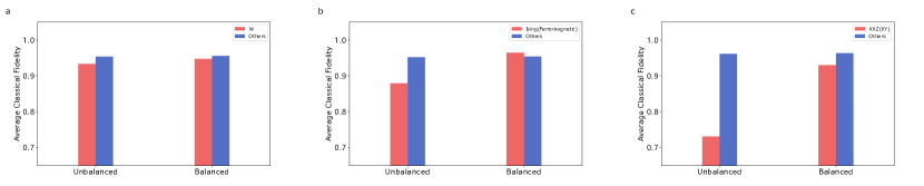
Figure 9: Performances of GQNQ when training data from different types of quantum states are unbalanced. In each figure, the red bar represents the classical fidelity with respect to the chosen underrepresented type of states, and the blue bar represents the classical fidelity averaged over all other types of states. Fig.(a) compares the average classical fidelity for W states with local rotations and the average classical fidelity for all other states when the ratio of the size of training data from W states to any other type is $1:10$ and $1:1$, respectively. Fig.(b) compares the average classical fidelity for ground states of ferromagnetic Ising model with the average classical fidelity for all other states when the ratio of the size of training data from ferromagnetic Ising model to any other type is $1:10$ and $1:1$, respectively. Fig.(c) compares the average classical fidelity for ground states of XXZ model in XY phase with the average classical fidelity for all other states when the ratio of the size of training data from XXZ model in XY phase to any other type is $1:10$ and $1:1$, respectively.

XI Additional Experiments

XI.1 Ising model

We study the performance of GQNQ for $10$-, $20$- and $50$-qubit Ising ground states when the measurements are nearest-neighbour two-qubit Pauli measurements. Different from the setting in the main text, here we choose $J_{i}$ as a Gaussian variable with mean value $J$ and variance $0.01$. Hence when $J$ is around $0$, both ferromagnetic interactions and antiferromagnetic interactions are present with high probability. We find that GQNQ cannot give good predictions of outcome statistics in this scenario when both ferromagnetic and antiferromagnetic interactions exist. The results, together with the comparison with the scenario where each $J_{i}$ is chosen to be the absolute value (or the opposite of the absolute value, for $J<0$) of the Gaussian variable, are presented in Fig. 10.

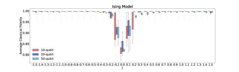
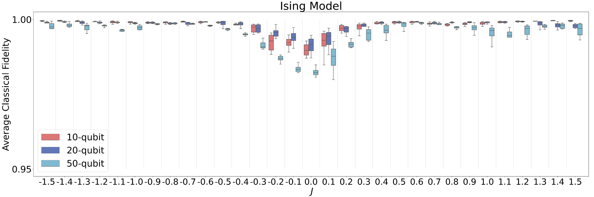
Figure 10: Comparison between the performances of GQNQ in Ising model when both ferromagnetic and antiferromagnetic interactions are present near $J=0$ (top) vs when only either ferromagnetic or antiferromagnetic interactions are present near $J=0$ (bottom).

XI.2 Cat states

For the numerical experiments on learning of continuous-variable quantum states, we provide an example of comparison between predictions and ground truths for a cat state in Fig. 11 here.

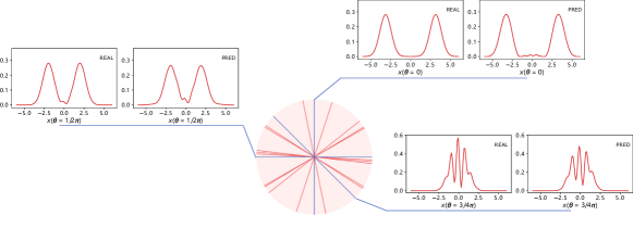
Figure 11: The true outcome probability density (left) and the predicted probability density (right) for cat state $\ket{2.22+1.41\text{i},\pi/4}_{\text{cat}}$ at quadrature phases $\theta=0$, $\theta=\pi/2$ and $\theta=3\pi/4$, respectively, given the measurement outcome densities at ten random quadrature phases. In the middle circle, ten red lines passing through the center represent those quadrature phases at which measurement outcome statistics are known, and three blue lines passing through the center represent those quadrature phases at which measurement outcome statistics are to be predicted.

XII Training with data from the state to be characterized

In this section, we discuss how to train our GQNQ model with data only from the quantum state to be characterized. In this setting, GQNQ behaves as a completely unsupervised learner that predicts the outcome statistics of unperformed measurements using measurement data obtained from the quantum state under consideration. The set $\mathcal{M}_{*}$ of fiducial measurements in the training coincides with the set $\mathcal{S}$ of performed measurements. In the training, GQNQ is trained with $s(s<n)$ measurement results $\{(\bm{m}_{i},\bm{p}_{i})\}_{i=1}^{s}$ corresponding to $\mathcal{S}$. When the training is finished, the trained model can be utilized to predict the outcome statistics corresponding to $\mathcal{M}\setminus\mathcal{S}$.

We present the whole training procedure in such setting by pseudocode in Algorithm 2.

Data: State measurement results $\{(\bm{m}_{i},\bm{p}_{i})\}_{i=1}^{s}$ of the quantum state to be characterized corresponding to the set of reference measurements $\mathcal{M}_{*}$ , maximum number of known POVM measurement results $a(a<s)$ in the training, maximum number of epochs $E$, learning rate $\delta$.

Initialize parameters $\bm{\xi}$ and $\bm{\eta}$ randomly, $e=0$;

while $e<E$ do

       $\mathcal{L}=0$;

       Generate a random integer number $n_{1}$ from $[1,a]$;

       Randomly select $n_{1}$ pairs of $(\bm{m}_{i},\bm{p}_{i})$ from $\{(\bm{m}_{i},\bm{p}_{i})\}_{i=1}^{s}$ and denote them as $\{(\bm{m}_{i_{j}},\bm{p}_{i_{j}})\}_{j=1}^{n_{1}}$, where $\{i_{j}\}_{j=1}^{s}$ is a permutation of $\{1,\dots,s\}$ ;

       Input each of $\{(\bm{m}_{i_{j}},\bm{p}_{i_{j}})\}_{j=1}^{n_{1}}$ into the representation network $f_{\bm{\xi}}$ to obtain the representations $\{\bm{r}_{i_{j}}\}_{j=1}^{n_{1}}$ as $\bm{r}_{i_{j}}=f_{\bm{\xi}}(\bm{m}_{i_{j}},\bm{p}_{i_{j}})$ ;

       Calculate the state representation by an aggregate function $\mathcal{A}$ as $\bm{r}=\mathcal{A}(\{\bm{r}_{i_{j}}\}_{j=1}^{n_{1}})$ ;

       Input $\bm{r}$ and the remaining $\{\bm{m}_{i_{j}}\}_{j=n_{1}+1}^{s}$ into the generation network $g_{\bm{\eta}}$ to obtain the predictions $\{\bm{p}^{\prime}_{i_{j}}\}_{j=n_{1}+1}^{s}$ of measurement outcome distributions as $\bm{p}^{\prime}_{i_{j}}=g_{\bm{\eta}}(\bm{r},\bm{m}_{i_{j}})$;

       Calculate the loss $l$ with Eq. (3) by comparing $\{\bm{p}^{\prime}_{i_{j}}\}_{j=n_{1}+1}^{s}$ with $\{\bm{p}_{i_{j}}\}_{j=n_{1}+1}^{s}$ and update $\mathcal{L}$ as $\mathcal{L}=\mathcal{L}+l$ ;

      

      Calculate $\nabla_{\bm{\xi}}\mathcal{L}$ and $\nabla_{\bm{\eta}}\mathcal{L}$ ;

       Update $\bm{\xi}$ and $\bm{\eta}$ as $\bm{\xi}=\bm{\xi}-\delta\nabla_{\bm{\xi}}\mathcal{L}$, $\bm{\eta}=\bm{\eta}-\delta\nabla_{\bm{\eta}}\mathcal{L}$ ;

       $\mathcal{L}=0$;

      

      $e=e+1$ ;

      

Algorithm 2 Training of GQNQ with data provided from the quantum state to be characterized.

References

- Eisert et al. (2020) Jens Eisert, Dominik Hangleiter, Nathan Walk, Ingo Roth, Damian Markham, Rhea Parekh, Ulysse Chabaud, and Elham Kashefi, “Quantum certification and benchmarking,” Nat. Rev. Phys. 2, 382–390 (2020).
- Tóth et al. (2010) G. Tóth, W. Wieczorek, D. Gross, R. Krischek, C. Schwemmer, and H. Weinfurter, “Permutationally invariant quantum tomography,” Phys. Rev. Lett. 105, 250403 (2010).
- Gross et al. (2010) David Gross, Yi-Kai Liu, Steven T. Flammia, Stephen Becker, and Jens Eisert, “Quantum state tomography via compressed sensing,” Phys. Rev. Lett. 105, 150401 (2010).
- Cramer et al. (2010) Marcus Cramer, Martin B Plenio, Steven T Flammia, Rolando Somma, David Gross, Stephen D Bartlett, Olivier Landon-Cardinal, David Poulin, and Yi-Kai Liu, “Efficient quantum state tomography,” Nat. Commun. 1, 1–7 (2010).
- Lanyon et al. (2017) BP Lanyon, C Maier, Milan Holzäpfel, Tillmann Baumgratz, C Hempel, P Jurcevic, Ish Dhand, AS Buyskikh, AJ Daley, Marcus Cramer, et al., “Efficient tomography of a quantum many-body system,” Nat. Phys. 13, 1158–1162 (2017).
- Cotler and Wilczek (2020) Jordan Cotler and Frank Wilczek, “Quantum overlapping tomography,” Phys. Rev. Lett. 124, 100401 (2020).
- Huang et al. (2020) Hsin-Yuan Huang, Richard Kueng, and John Preskill, “Predicting many properties of a quantum system from very few measurements,” Nat. Phys. 16, 1050–1057 (2020).
- Huang et al. (2021) Hsin-Yuan Huang, Richard Kueng, Giacomo Torlai, Victor V Albert, and John Preskill, “Provably efficient machine learning for quantum many-body problems,” arXiv:2106.12627 (2021).
- Flammia and Liu (2011) Steven T. Flammia and Yi-Kai Liu, “Direct fidelity estimation from few pauli measurements,” Phys. Rev. Lett. 106, 230501 (2011).
- da Silva et al. (2011) Marcus P. da Silva, Olivier Landon-Cardinal, and David Poulin, “Practical characterization of quantum devices without tomography,” Phys. Rev. Lett. 107, 210404 (2011).
- Aaronson (2007) Scott Aaronson, “The learnability of quantum states,” Proc. R. Soc. A 463, 3089–3114 (2007).
- Aaronson (2019) Scott Aaronson, “Shadow tomography of quantum states,” SIAM J. Comput. 49, STOC18–368 (2019).
- Aaronson et al. (2019) Scott Aaronson, Xinyi Chen, Elad Hazan, Satyen Kale, and Ashwin Nayak, “Online learning of quantum states,” J. Stat. Mech.: Theory Exp. 2019, 124019 (2019).
- Arunachalam et al. (2020) Srinivasan Arunachalam, Alex B Grilo, and Henry Yuen, “Quantum statistical query learning,” arXiv:2002.08240 (2020).
- Carleo et al. (2019) Giuseppe Carleo, Ignacio Cirac, Kyle Cranmer, Laurent Daudet, Maria Schuld, Naftali Tishby, Leslie Vogt-Maranto, and Lenka Zdeborová, “Machine learning and the physical sciences,” Rev. Mod. Phys. 91, 045002 (2019).
- Torlai et al. (2018) Giacomo Torlai, Guglielmo Mazzola, Juan Carrasquilla, Matthias Troyer, Roger Melko, and Giuseppe Carleo, “Neural-network quantum state tomography,” Nat. Phys. 14, 447–450 (2018).
- Torlai and Melko (2018) Giacomo Torlai and Roger G. Melko, “Latent space purification via neural density operators,” Phys. Rev. Lett. 120, 240503 (2018).
- Xu and Xu (2018) Qian Xu and Shuqi Xu, “Neural network state estimation for full quantum state tomography,” arXiv preprint arXiv:1811.06654 (2018).
- Carrasquilla et al. (2019) Juan Carrasquilla, Giacomo Torlai, Roger G Melko, and Leandro Aolita, “Reconstructing quantum states with generative models,” Nat. Mach. Intell. 1, 155–161 (2019).
- Tiunov et al. (2020) Egor S Tiunov, VV Tiunova, Alexander E Ulanov, AI Lvovsky, and Aleksey K Fedorov, “Experimental quantum homodyne tomography via machine learning,” Optica 7, 448–454 (2020).
- Ahmed et al. (2021a) Shahnawaz Ahmed, Carlos Sánchez Muñoz, Franco Nori, and Anton Frisk Kockum, “Quantum state tomography with conditional generative adversarial networks,” Phys. Rev. Lett. 127, 140502 (2021a).
- Ahmed et al. (2021b) Shahnawaz Ahmed, Carlos Sánchez Muñoz, Franco Nori, and Anton Frisk Kockum, “Classification and reconstruction of optical quantum states with deep neural networks,” Phys. Rev. Res. 3, 033278 (2021b).
- Rocchetto et al. (2018) Andrea Rocchetto, Edward Grant, Sergii Strelchuk, Giuseppe Carleo, and Simone Severini, “Learning hard quantum distributions with variational autoencoders,” NPJ Quantum Inf. 4, 28 (2018).
- Quek et al. (2021) Yihui Quek, Stanislav Fort, and Hui Khoon Ng, “Adaptive quantum state tomography with neural networks,” NPJ Quantum Inf. 7, 105 (2021).
- Palmieri et al. (2020) Adriano Macarone Palmieri, Egor Kovlakov, Federico Bianchi, Dmitry Yudin, Stanislav Straupe, Jacob D Biamonte, and Sergei Kulik, “Experimental neural network enhanced quantum tomography,” NPJ Quantum Inf. 6, 20 (2020).
- Smith et al. (2021) Alistair W. R. Smith, Johnnie Gray, and M. S. Kim, “Efficient quantum state sample tomography with basis-dependent neural networks,” PRX Quantum 2, 020348 (2021).
- Sentís et al. (2019) Gael Sentís, Alex Monràs, Ramon Muñoz Tapia, John Calsamiglia, and Emilio Bagan, “Unsupervised classification of quantum data,” Phys. Rev. X 9, 041029 (2019).
- Gao et al. (2018) Jun Gao, Lu-Feng Qiao, Zhi-Qiang Jiao, Yue-Chi Ma, Cheng-Qiu Hu, Ruo-Jing Ren, Ai-Lin Yang, Hao Tang, Man-Hong Yung, and Xian-Min Jin, “Experimental machine learning of quantum states,” Phys. Rev. Lett. 120, 240501 (2018).
- Elben et al. (2020) Andreas Elben, Benoît Vermersch, Rick van Bijnen, Christian Kokail, Tiff Brydges, Christine Maier, Manoj K. Joshi, Rainer Blatt, Christian F. Roos, and Peter Zoller, “Cross-platform verification of intermediate scale quantum devices,” Phys. Rev. Lett. 124, 010504 (2020).
- Eslami et al. (2018) SM Ali Eslami, Danilo Jimenez Rezende, Frederic Besse, Fabio Viola, Ari S Morcos, Marta Garnelo, Avraham Ruderman, Andrei A Rusu, Ivo Danihelka, Karol Gregor, et al., “Neural scene representation and rendering,” Science 360, 1204–1210 (2018).
- Bengio et al. (2013) Yoshua Bengio, Aaron Courville, and Pascal Vincent, “Representation learning: A review and new perspectives,” IEEE Trans. Pattern Anal. Mach. Intell. 35, 1798–1828 (2013).
- Foster (2019) David Foster, Generative deep learning: teaching machines to paint, write, compose, and play (O’Reilly Media, 2019).
- Teo et al. (2011) Yong Siah Teo, Huangjun Zhu, Berthold-Georg Englert, Jaroslav Řeháček, and Zden ěk Hradil, “Quantum-state reconstruction by maximizing likelihood and entropy,” Phys. Rev. Lett. 107, 020404 (2011).
- Schollwöck et al. (2008) Ulrich Schollwöck, Johannes Richter, Damian JJ Farnell, and Raymond F Bishop, Quantum magnetism, Vol. 645 (Springer, 2008).
- Samaj (2013) Ladislav Samaj, Introduction to the statistical physics of integrable many-body systems (Cambridge University Press, 2013).
- Friedenauer et al. (2008) Axel Friedenauer, Hector Schmitz, Jan Tibor Glueckert, Diego Porras, and Tobias Schätz, “Simulating a quantum magnet with trapped ions,” Nat. Phys. 4, 757–761 (2008).
- Kim et al. (2010) Kihwan Kim, M-S Chang, Simcha Korenblit, Rajibul Islam, Emily E Edwards, James K Freericks, G-D Lin, L-M Duan, and Christopher Monroe, “Quantum simulation of frustrated ising spins with trapped ions,” Nature 465, 590–593 (2010).
- Islam et al. (2011) R Islam, EE Edwards, K Kim, S Korenblit, C Noh, H Carmichael, G-D Lin, L-M Duan, C-C Joseph Wang, JK Freericks, et al., “Onset of a quantum phase transition with a trapped ion quantum simulator,” Nat. Commun. 2, 1–6 (2011).
- Yang and Yang (1966) C. N. Yang and C. P. Yang, “One-dimensional chain of anisotropic spin-spin interactions. i. proof of bethe’s hypothesis for ground state in a finite system,” Phys. Rev. 150, 321–327 (1966).
- Williamson et al. (1989) David F Williamson, Robert A Parker, and Juliette S Kendrick, “The box plot: a simple visual method to interpret data,” Annals of internal medicine 110, 916–921 (1989).
- Gottesman et al. (2001) Daniel Gottesman, Alexei Kitaev, and John Preskill, “Encoding a qubit in an oscillator,” Phys. Rev. A 64, 012310 (2001).
- Albert et al. (2018) Victor V. Albert, Kyungjoo Noh, Kasper Duivenvoorden, Dylan J. Young, R. T. Brierley, Philip Reinhold, Christophe Vuillot, Linshu Li, Chao Shen, S. M. Girvin, Barbara M. Terhal, and Liang Jiang, “Performance and structure of single-mode bosonic codes,” Phys. Rev. A 97, 032346 (2018).
- Van der Maaten and Hinton (2008) Laurens Van der Maaten and Geoffrey Hinton, “Visualizing data using t-sne.” Journal of machine learning research 9 (2008).
- Bishop and Nasrabadi (2006) Christopher M Bishop and Nasser M Nasrabadi, Pattern recognition and machine learning, Vol. 4 (Springer, 2006).
- Iten et al. (2020) Raban Iten, Tony Metger, Henrik Wilming, Lídia del Rio, and Renato Renner, “Discovering physical concepts with neural networks,” Phys. Rev. Lett. 124, 010508 (2020).
- Schollwöck (2005) Ulrich Schollwöck, “The density-matrix renormalization group,” Reviews of modern physics 77, 259 (2005).
- Killoran et al. (2019) Nathan Killoran, Josh Izaac, Nicolás Quesada, Ville Bergholm, Matthew Amy, and Christian Weedbrook, “Strawberry fields: A software platform for photonic quantum computing,” Quantum 3, 129 (2019).
- Kingma and Ba (2014) Diederik P Kingma and Jimmy Ba, “Adam: A method for stochastic optimization,” arXiv preprint arXiv:1412.6980 (2014).
- Paszke et al. (2019) Adam Paszke, Sam Gross, Francisco Massa, Adam Lerer, James Bradbury, Gregory Chanan, Trevor Killeen, Zeming Lin, Natalia Gimelshein, Luca Antiga, et al., “Pytorch: An imperative style, high-performance deep learning library,” Advances in neural information processing systems 32, 8026–8037 (2019).
- Aggarwal et al. (2018) Charu C Aggarwal et al., “Neural networks and deep learning,” Springer 10, 978–3 (2018).
- Hochreiter and Schmidhuber (1997) Sepp Hochreiter and Jürgen Schmidhuber, “Long short-term memory,” Neural computation 9, 1735–1780 (1997).
- Kullback (1997) Solomon Kullback, Information theory and statistics (Courier Corporation, 1997).
- Ruder (2016) Sebastian Ruder, “An overview of gradient descent optimization algorithms,” arXiv preprint arXiv:1609.04747 (2016).
- Leonhardt (1997) Ulf Leonhardt, Measuring the quantum state of light, Vol. 22 (Cambridge university press, 1997).