Tight integration of neural- and clustering-based diarization
through deep unfolding of infinite Gaussian mixture model

Abstract

Speaker diarization has been investigated extensively as an important central task for meeting analysis. Recent trend shows that integration of end-to-end neural (EEND)- and clustering-based diarization is a promising approach to handle realistic conversational data containing overlapped speech with an arbitrarily large number of speakers, and achieved state-of-the-art results on various tasks. However, the approaches proposed so far have not realized tight integration yet, because the clustering employed therein was not optimal in any sense for clustering the speaker embeddings estimated by the EEND module. To address this problem, this paper introduces a trainable clustering algorithm into the integration framework, by deep-unfolding a non-parametric Bayesian model called the infinite Gaussian mixture model (iGMM). Specifically, the speaker embeddings are optimized during training such that it better fits iGMM clustering, based on a novel clustering loss based on Adjusted Rand Index (ARI). Experimental results based on CALLHOME data show that the proposed approach outperforms the conventional approach in terms of diarization error rate (DER), especially by substantially reducing speaker confusion errors, that indeed reflects the effectiveness of the proposed iGMM integration.

Index Terms—  Diarization, deep learning, infinite GMM

1 Introduction

Automatic meeting/conversation analysis is one of the essential technologies required for realizing futuristic speech applications such as communication agents that can follow, respond to, and facilitate our conversations. As an important central task for the meeting analysis, speaker diarization has been extensively studied [1, 2, 3].

Current competitive diarization approaches can be categorized into three types; speaker embedding clustering-based approaches [4, 1, 5, 6], neural end-to-end diarization (EEND) approaches [7, 8, 9], and combination/integration of the former two approaches [10, 11, 12, 13]. The speaker embedding clustering-based approaches first segment a recording into short homogeneous chunks and compute speaker embeddings such as x-vectors [4] for each chunk assuming that only one speaker is active in each chunk. Then, the speaker embeddings are clustered to regroup segments belonging to the same speakers and obtain the diarization results. While these methods can cope with very challenging scenarios [5, 6] and work with an arbitrarily large number of speakers, there is a clear disadvantage that they cannot handle overlapped speech.

The second category of diarization approaches, EEND, was recently developed [7, 8, 9] to specifically address the overlapped speech problem. Similarly to the neural source separation [14, 15], a Neural Network (NN) receives frame-level spectral features and directly outputs a frame-level speaker activity for each speaker, no matter whether the input signal contains overlapped speech or not. While the system is simple and has started outperforming the conventional clustering-based algorithms [8, 9], it still has difficulty in generalizing to recordings containing a large number of speakers [9].

To this end, the third category of diarization approaches, integration of the EEND- and clustering-based approaches [10, 11, 12, 13], referred to as EEND-vector clustering (EEND-VC) hereafter, has been recently proposed to cope with realistic recordings containing overlapped speech with an arbitrarily large number of speakers. It first splits the input recording into fixed-length chunks. Then, it applies a modified version of EEND to each chunk to obtain diarization results for speakers speaking in each chunk as well as speaker embeddings for them. Finally, to estimate which of the diarization results estimated in local chunks belongs to the same speaker, speaker clustering is performed across the chunks based on the speaker embeddings by using a constrained clustering algorithm. While this integrated approach is shown to achieve state-of-the-art results for real conversational data such as CALLHOME data [10, 12], we argue that there is a large room for improvement because the integration is not tight enough; Although the estimation of diarization results and speaker embeddings is based on a single NN and thus are tightly coupled, the clustering stage is formulated as an independent process that is not guaranteed to be optimal in clustering the speaker embeddings, and thus the overall system could not be optimal.

To address this problem and tightly integrate EEND- and clustering-based diarization, this paper introduces a trainable clustering framework, unfolded infinite Gaussian mixture model (iGMM) [16], into the EEND-VC framework. Desired properties of a clustering algorithm for EEND-VC are (1) it should deal with arbitrary unbounded number of speakers, (2) it should estimate the number of speakers in an optimal sense, (3) it should handle non-sequential data (unlike [17]) because a set of the speaker embeddings in the EEND-VC framework has no specific order. As a typical clustering algorithm that fulfills these conditions, we propose to employ a non-parametric Bayesian model called iGMM, which is a GMM but with a theoretically infinite number of mixture components. The number of mixture components, corresponding to the number of speakers in diarization, can be optimized in a maximum marginal likelihood sense, given an observation. To jointly optimize this novel clustering step with speaker embedding estimation and diarization results estimation, we opt to unfold the parameter estimation process of iGMM and optimize directly the clustering results through a novel adjusted Rand index (ARI)-based loss [16]. Experiments based on CALLHOME data show the proposed approach can outperform the conventional EEND-VC in terms of diarization error rate (DER) especially by reducing speaker confusion errors, which indeed reflects the effectiveness of the proposed iGMM integration.

Fig. 1: Schematic diagram of the proposed diarization framework. The input contains 3 speakers in total (red, green, and blue speakers shown in the waveform at the bottom), but only at most 2 speakers are actively speaking in each chunk.

Fig. 2: Proposed neural network architecture and loss functions for neural network optimization

2 Proposed Diarization framework

2.1 Overall framework

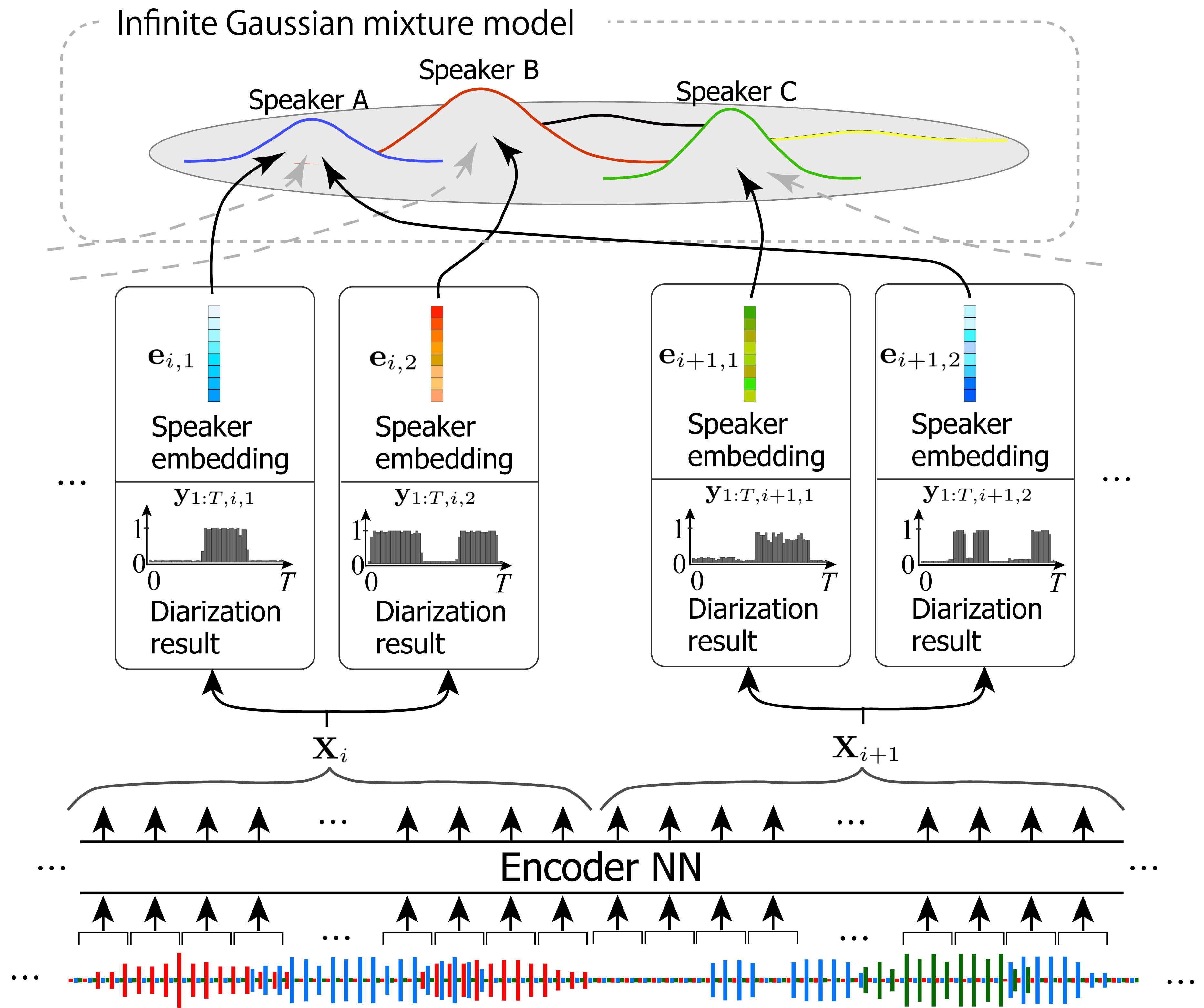
Figure 1 shows a schematic diagram of the proposed framework, EEND-vector clustering with iGMM (EEND-VC-iGMM), for an exemplary 2 chunks out of continuous 3-speaker meeting data.

It first passes a several-minute long input recording to NN (“Encoder NN” in Fig. 1), and obtain a set of $D$-dimensional frame features. Then, these features are segmented into chunks to form chunk-level features, as $\mathbf{X}_{i}=(\mathbf{x}_{t,i}\in\mathbb{R}^{D}\mid t=1,\cdots,T)$ where $i$, $t$ and $T$ are the chunk index, the frame index in the chunk and the chunk size. In the following explanation, we assume that we can reasonably fix the maximum number of active speakers in a chunk, $S_{\textrm{Local}}$, to 2, for the sake of simplicity .

With the assumption/hyper-parameter $S_{\textrm{Local}}=2$ and $\mathbf{X}_{i}$, the system estimates, based on an NN, diarization results and speaker embeddings associated with the 2 speakers in each chunk. If a speaker is absent (i.e., there is only one active speaker in that chunk), the network simply estimates the diarization results of all zeros for that silent speaker. Since it is not always guaranteed that the diarization results of a certain speaker are estimated at the same output node, we may have the inter-chunk label permutation problem in the diarization outputs [10, 18]. We can solve this permutation problem and estimate the correct association of the diarization results among chunks, by clustering the speaker embeddings given the total number of speakers in the input recording, $S_{\textrm{Global}}$, (3 in the example shown in Fig. 1), or given an estimate of $S_{\textrm{Global}}$.

In the previous studies [11, 12], the speaker embedding extraction process is optimized such that vectors of the same speaker stay close to each other, while those from different speakers lie far away from each other, based on a categorical cross-entropy loss [11] or a contrastive loss [12]. Then, the obtained embeddings are clustered into each speaker, utilizing constrained clustering algorithms such as constrained Agglomerative Hierarchical Clustering (AHC). In other words, the embeddings were not optimized for clustering.

In this paper, we propose to train speaker embeddings such that they can be well modeled by a non-parametric Bayesian model called iGMM. By having this clustering process not only in the inference but also in the training, we can tightly integrate the speaker embedding estimation and the subsequent clustering processes.

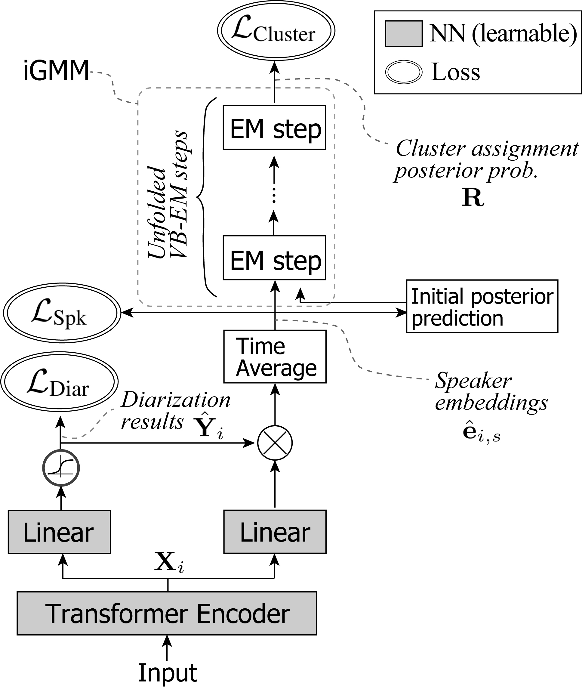
In the next subsections, we will detail essential components of EEND-VC-iGMM by using Fig. 2, which summarizes an NN processing flow and loss functions used in the proposed framework.

2.2 Chunk-wise diarization and speaker embedding estimation

The lower part of Fig. 2 corresponds to the chunk-wise estimation of diarization results and speaker embeddings. First let us denote the ground-truth diarization labels at each $i$-th chunk as $\mathbf{Y}_{i}=\{\mathbf{y}_{t,i}\mid t=1,\cdots,T\}\in\mathbb{R}^{S_{\textrm{Local}}\times T}$ that corresponds to $\mathbf{X}_{i}$, and $C$-dimensional speaker embeddings estimated at the $i$-th chunk for the $s$-th speaker as $\hat{\mathbf{e}}_{i,s}\in\mathbb{R}^{C}$. Here, the diarization label $\mathbf{y}_{t,i}=[y_{t,i,s}\in\{0,1\}\mid s=1,\cdots,S_{\textrm{Local}}]$ represents a joint activity for $S_{\textrm{Local}}$ speakers. For example, $y_{t,i,s}=y_{t,i,s^{\prime}}=1(s\neq s^{\prime})$ indicates both speakers $s$ and $s^{\prime}$ spoke at the time frame $t$ in the chunk $i$. Then, after obtaining $\{\mathbf{X}_{i}\}_{i=1}^{I}$ for all $I$ chunks by processing input speech with a Transformer encoder, we can jointly estimate diarization results and speaker embeddings at the $i$-th chunk as:

$$\vspace{-1mm}\hat{\mathbf{Y}}_{i}=\sigma(\mathrm{Linear}(\mathbf{X}_{i})),\ \ \hat{\mathbf{e}}_{i,1},\ldots,\hat{\mathbf{e}}_{i,S_{\textrm{Local}}}=\mathrm{Avg}_{\hat{\mathbf{Y}}_{i}}(\mathrm{Linear}(\mathbf{X}_{i})).\vspace{-1mm}$$

$\sigma(\cdot)$, $\mathrm{Linear}(\cdot)$ and $\mathrm{Avg}_{\mathbf{A}}(\cdot)$ are the sigmoid activation function, linear layers, and a time-averaging function with a time-varying weight $\mathbf{A}$, respectively.

2.3 Infinite Gaussian mixture model and its deep unfolding

After estimating a set of speaker embeddings $\{\{\hat{\mathbf{e}}_{i,s}\}_{s=1}^{S_{\textrm{Local}}}\}_{i=1}^{I}$, we cluster them with an iGMM, which is a special case of Dirichlet process (DP) mixture models. The upper right part of Fig. 2 corresponds to the speaker embedding clustering process by iGMM. iGMM theoretically has an infinite number of Gaussian components, and uses a part of them to appropriately model observation data. The clustering and the number of cluster estimation are jointly done in a maximum marginal likelihood sense by means of variational Bayesian (VB) inference of the model parameters given observed data.

Specifically, the proposed iGMM takes a set of speaker embeddings as an input, and outputs soft speaker-cluster assignments $\mathbf{R}=\{\{\mathbf{r}_{i,s}\}_{s=1}^{S_{\textrm{Local}}}\}_{i=1}^{I}$, where $\mathbf{r}_{i,s}=\{r_{i,s,k}\}_{k=1}^{K^{\prime}}$. $r_{i,s,k}$ is the probability that the speaker embedding $\hat{\mathbf{e}}_{i,s}$ is assigned to the $k$-th cluster, and $K^{\prime}$ is the maximum number of clusters, which is set at a large value in practice.

2.3.1 Generative process of the speaker embeddings

First, let us explain the generative process assumed in the proposed iGMM. For the sake of convenience, let us introduce a variable $N$ that corresponds to the total number of input speaker embeddings, i.e., $N=I\times S_{\textrm{Local}}$, and an index for the embeddings, $n$, such as $\mathbf{e}_{n}$ . Then, in this paper, we employ a spherical iGMM with the following generative process for the speaker embeddings, where the mixture weights are constructed by a DP prior with concentration parameter $\alpha$ by a stick-breaking process [19], as:

1. For each speaker cluster $k=1,\cdots,\infty$

   1. Draw stick proportion $\eta_{k}\sim\mathrm{Beta}(1,\alpha)$

   2. Set mixture weight $\pi_{k}=\eta_{k}\prod_{k^{\prime}=1}^{k-1}(1-\eta_{k^{\prime}})$

   3. Draw cluster mean $\bm{\mu}_{k}\sim\mathcal{N}(\mathbf{0},\mathbf{I})$

   4. Draw cluster precision $\beta_{k}\sim\mathrm{Gamma}(1,1)$

2. For each speaker embedding $n=1,\cdots,N$

   1. Draw cluster assignment
      $v_{n}\sim\mathrm{Categorical}(\bm{\pi})$

   2. Draw instance representation
      $\mathbf{e}_{n}=\mathcal{N}(\bm{\mu}_{v_{n}},\beta_{v_{n}}^{-1}\mathbf{I})$

$\mathrm{Beta}$ is the beta distribution, $\mathcal{N}(\bm{\mu},\bm{\Sigma})$ is the Gaussian distribution with mean $\bm{\mu}$ and covariance $\bm{\Sigma}$, $\mathrm{Gamma}$ is the gamma distribution, $\mathrm{Categorical}$ is the categorical distribution, and $\bm{\pi}=\{\pi_{k}\}_{k=1}^{\infty}$. The DP prior by a stick-breaking process (steps 1-(a) and 1-(b)) is a key to allow us to use the infinite number of mixture components.

2.3.2 Parameter estimation for iGMM

Following the above generative process, we can derive the following parameter estimation steps based on the VB expectation-maximization (EM) algorithm. Because of the space limitation, the derivation of the following equations is omitted, but it follows a straight-forward procedure of maximizing an evidence lower bound derived from the iGMM likelihood as shown in [16]. The iGMM parameter estimation in the variational posterior distributions is achieved by alternately calculating the following VB M-step:

$$\vspace{-2mm}\gamma_{k1} =1+\sum_{n=1}^{N}r_{n,k},\quad\gamma_{k2}=\alpha+\sum_{n=1}^{N}\sum_{k^{\prime}=k+1}^{K^{\prime}}r_{n,k^{\prime}},\quad$$

$$\bm{\theta}_{k} =\frac{\frac{b_{k}}{a_{k}}\sum_{n=1}^{N}r_{n,k}\mathbf{e}_{n}}{1+\frac{b_{k}}{a_{k}}\sum_{n=1}^{N}r_{n,k}},$$

$$a_{k} =1+\frac{C}{2}\sum_{n=1}^{N}r_{n,k},\quad b_{k}=1+\frac{1}{2}\sum_{n=1}^{N}r_{n,k}(\parallel\mathbf{e}_{n}-\bm{\theta}_{k}\parallel^{2}+C),$$

and the following VB E-step to obtain a cluster assignment $r_{n,k}$:

$$\log r_{n,k}\propto\Psi(\gamma_{k1})-\Psi(\gamma_{k1}+\gamma_{k2})-\frac{C}{2}(\Psi(a_{k})-\log(b_{k}))$$

$$-\frac{a_{k}}{2b_{k}}(\parallel\mathbf{e}_{n}-\bm{\theta}_{k}\parallel^{2}+C)+\sum_{k^{\prime}=k+1}^{K^{\prime}}(\Psi(\gamma_{k2})-\Psi(\gamma_{k1}+\gamma_{k2})),\vspace{-1mm}$$

where $\Psi$ is the digamma function. For the computational efficiency, we truncate the number of clusters at $K^{\prime}$ as in [20]. Note that the truncated DP is shown to closely approximate a true DP for large enough $K^{\prime}$ relative to the number of samples [21].

Since [16] shows that, to help the VB EM steps converge faster to a better solution, it is beneficial to estimate an initial value of the posterior probability $\mathbf{R}$ with another small NN, we also employ such a small network, which corresponds to a block denoted as “Initial posterior prediction” in Fig. 2. Its details are summarized in [16].

2.3.3 Deep unfolding of iGMM parameter estimation process

The above VB EM steps are all clearly differentiable. Thus, by following an idea of general deep unfolding framework, e.g., [22], we unfold the EM iterations into a sequential processing as in the upper right part of Fig. 2 to incorporate iGMM-based clustering into the overall NN optimization framework.

2.4 Loss functions

Now, let us explain how we optimize the network. As it is shown in Fig. 2, the system can be optimized by the following multi-task loss;

$$\vspace{-1mm}\mathcal{L} = (1-\lambda_{1}-\lambda_{2})\mathcal{L}_{\textrm{Diar}}+\lambda_{1}\mathcal{L}_{\textrm{Cluster}}+\lambda_{2}\mathcal{L}_{\textrm{Spk}},\vspace{-1mm}$$ (1)

where $\mathcal{L}_{\textrm{Diar}}$, $\mathcal{L}_{\textrm{Cluster}}$, $\mathcal{L}_{\textrm{Spk}}$ correspond to losses that control chunk-wise diarization accuracy, clustering accuracy, and a speaker embedding space to have small intra-speaker and large inter-speaker variability, respectively. $\mathcal{W}=\{\lambda_{1},\lambda_{2}\}$ includes weights for the multi-task loss. In the following, we will detail $\mathcal{L}_{\textrm{Diar}}$ and $\mathcal{L}_{\textrm{Cluster}}$, while we ask readers to refer to [10] for details of $\mathcal{L}_{\textrm{Spk}}$. $\mathcal{L}_{\textrm{Spk}}$ in this paper is based on absolute speaker identity labels.

Table 1: DERs (%) of EEND-VC and the proposed EEND-VC-iGMM for the different number of speakers in the CALLHOME evaluation set. The numbers in parentheses indicate the missed detection (MI), false alarm (FA) and speaker confusion (CF) errors, i.e., (MI/FA/CF).

Model	$\mathcal{L}_{\textrm{Spk}}$	Number of speakers in a recording
		2	3	4	5	6	Avg.
EEND-VC	✓	7.0 (4.0/2.4/0.5)	14.2 (4.9/3.5/5.8)	16.7 (6.0/2.7/8.0)	31.6 (8.0/2.4/21.2)	29.9 (10.9/3.5/15.5)	13.8 (5.6/2.7/5.5)
EEND-VC-iGMM	-	8.1 (4.6/2.7/1.1)	12.3 (5.2/3.6/3.5)	18.0 (6.4/4.4/7.1)	28.4 (6.3/4.7/17.3)	33.8 (11.1/4.8/17.9)	13.7 (6.5/2.7/4.5)
EEND-VC-iGMM	✓	8.6 (4.8/2.3/1.4)	12.6 (6.6/2.3/3.6)	16.1 (6.4/3.7/6.1)	27.5 (5.3/4.9/17.3)	26.9 (11.9/3.2/11.4)	13.3 (5.2/3.6/4.5)

2.4.1 Chunk-level diarization loss

As in [7], the diariation loss $\mathcal{L}_{\textrm{Diar}}$ in each chunk is formulated as:

$$\vspace{-2mm}\mathcal{L}_{\textrm{Diar},i} = \frac{1}{TS_{\textrm{Local}}}\min_{\phi\in\mathrm{perm}(S_{\textrm{Local}})}\sum_{t=1}^{T}\textrm{BCE}\left(\mathbf{l}_{t,i}^{\phi},\hat{\mathbf{y}}_{t,i}\right),\vspace{-1mm}$$ (2)

where $\mathrm{perm}(S_{\textrm{Local}})$ is the set of all the possible permutations of ($1,\dots,S_{\textrm{Local}}$), $\hat{\mathbf{y}}_{t,i}=[\hat{y}_{t,i,1},\ldots,\hat{y}_{t,i,S_{\textrm{Local}}}]\in\mathbb{R}^{S_{\textrm{Local}}}$, $\mathbf{l}_{t,i}^{\phi}$ is the $\phi$-th permutation of the reference speaker labels, and $\mathrm{BCE}(\cdot,\cdot)$ is the binary cross-entropy function between the labels and the estimated diarization outputs.

2.4.2 Clustering loss: Adjusted Rand index loss

A common practice to evaluate clustering accuracy is to use the ARI [23, 24, 25], that directly measures similarity between a ground-truth clustering result and an estimated one, even when the estimated and true number of clusters does not agree. We here propose to use the (negative) ARI as a loss to directly improve the accuracy of the iGMM-based speaker embedding clustering, i.e., the accuracy of the posterior probability $\mathbf{R}$ obtained in 2.3.2.

Specifically, we use the following continuous approximation of ARI [16] (hereafter, cARI) that can handle soft cluster assignments, as opposed to the original non-differentiable ARI. Let us first define $N_{1}$ as the approximated number of pairs of instances (i.e., speaker embeddings) that are in different clusters in both the true and estimated assignments, $N_{2}$ as the approximated number of pairs that are in different clusters in the true assignments but not in the estimated assignments, $N_{3}$ as the approximated number of pairs that are in the same cluster in the true assignments but not in the estimated assignments, and $N_{4}$ as the approximated number of pairs that are in the same cluster in both the true and estimated assignments. Then, cARI is formulated as:

$$\mathrm{cARI}=\frac{2(N_{1}N_{4}-N_{2}N_{3})}{(N_{1}+N_{2})(N_{3}+N_{4})+(N_{1}+N_{3})(N_{2}+N_{4})},$$ (3)

where $N_{i}(i=1,\ldots,4)$ is mathematically defined as:

$$\vspace{-1mm}N_{1} =\sum_{n=1}^{N}\sum_{n^{\prime}=n+1}^{N}I(h_{n}\neq h_{n^{\prime}})d_{n,n^{\prime}},\vspace{-1mm}$$ (4)

$$N_{2} =\sum_{n=1}^{N}\sum_{n^{\prime}=n+1}^{N}I(h_{n}\neq h_{n^{\prime}})(1-d_{n,n^{\prime}}),\vspace{-1mm}$$ (5)

$$N_{3} =\sum_{n=1}^{N}\sum_{n^{\prime}=n+1}^{N}I(h_{n}=h_{n^{\prime}})d_{n,n^{\prime}},\vspace{-1mm}$$ (6)

$$N_{4} =\sum_{n=1}^{N}\sum_{n^{\prime}=n+1}^{N}I(h_{n}=h_{n^{\prime}})(1-d_{n,n^{\prime}}),\vspace{-1mm}$$ (7)

where $h_{n}$ is the true cluster assignment label for the $n$-th speaker embedding $\mathbf{e}_{n}$, $I(\cdot)$ is the indicator function, i.e., $I(A)$=1 if $A$ is true and $0$ otherwise, and $d_{n,n^{\prime}}$ is the total variation distance [26] between $\mathbf{r}_{n}$ and $\mathbf{r}_{n^{\prime}}$ defined as:

$$\vspace{-1mm}d_{n,n^{\prime}}=\frac{1}{2}\sum_{k=1}^{K^{\prime}}|r_{n,k}-r_{n^{\prime},k}|.\vspace{-1mm}$$ (8)

As a loss function $\mathcal{L}_{\textrm{Cluster}}$, we minimize $\mathcal{L}_{\textrm{Cluster}}=-\mathrm{cARI}$.

3 Experiments

Here, we evaluate the effectiveness of the proposed EEND-VC-iGMM on the widely used CALLHOME (CH) dataset [27, 1].

3.1 Data

We trained the diarization systems on simulated mixtures using speech from Switchboard-2, Switchboard Cellular, and the NIST Speaker Recognition Evaluations, and noise from the MUSAN corpus [28], and simulated room impulse responses from [29].

We generated 2 sets of training data. The first set (6.9k hours) consists of 1-to-3-speaker meeting-like data generated based on the algorithm proposed in [7] with $\beta=10$. This is the same training dataset as the one we used in [11]. We used it to train a seed model that was common for our baseline and proposed systems. The second training data (5.5k hours) consists of mixtures of up to 7 speakers, which simulates meetings with a larger number of speakers.

We evaluated the diarization systems on the CH dataset [27] that contains 500 telephone-conversation sessions including 2 to 6 speakers. Because there is a mismatch between the training and testing conditions, we used a part of the CH data for adaptation. We use the adaptation/evaluation data split proposed in [9].

3.2 Experimental settings

We evaluate the proposed EEND-VC-iGMM in comparison with the original EEND-VC with constrained AHC [11]. Both systems use the same configuration for the input feature, the Transformer encoder network, and the same silent speaker detection, all of which follow [11]. The only difference comes from the clustering modules, i.e., constrained AHC versus trainable iGMM. We assume a maximum number of speakers per chunk to be 3, i.e., $S_{\mathrm{local}}=3$. NN of the EEND-VC was trained with the multi-task weight of $\mathcal{W}=\{0.0,0.03\}$. We prepared two variants of EEND-VC-iGMM, one with the speaker embedding loss $\mathcal{L}_{\textrm{Spk}}$ based on absolute speaker identify labels, and one without it, by setting $\mathcal{W}=\{0.05,0.03\}$ and $\mathcal{W}=\{0.05,0.0\}$, respectively.

The training procedure is as follows. We first created the seed model using the 1-to-3-speaker training data and 30 seconds chunks for 100 epochs. We then re-trained the baseline EEND-VC and proposed EEND-VC-iGMM on the 2-to-7-speaker training data with 5-second chunks, i.e., $T=5~{}s$. These chunks are taken from 100 s and 300 s consecutive recordings for EEND-VC and EEND-VC-iGMM, respectively. Finally, we performed adaption using the CALLHOME adaptation data. For adaptation, we cut the recordings to 100 s for the baseline and 600 s for the proposed method, which corresponds to the optimal setting for each. This setting allows EEND-VC-iGMM to have sufficient number of embedding samples for the iGMM clustering during training. For the iGMM, we set the number of EM iterations at 10, $\alpha$ at 1, $K^{\prime}$ at 10, in both training and inference stages.

The performance was evaluated including overlapped speech frames in terms of DER with a collar tolerance of 0.25 s as in [9, 1].

3.3 Results

Table 1 shows the DERs for the conventional EEND-VC, and EEND-VC-iGMM with and without the speaker embedding loss $\mathcal{L}_{\textrm{Spk}}$. We can see that EEND-VC-iGMM outperforms EEND-VC in all but the 2-speaker condition. By looking at the breakdown of DERs, we observe that EEND-VC-iGMM greatly reduces speaker confusion errors in most cases. This clearly confirms the effectiveness of incorporating the trainable iGMM-based clustering and tightly coupling the embedding estimation and the clustering stages.

Looking at Avg. conditions, we can see that EEND-VC-iGMM with the speaker embedding loss $\mathcal{L}_{\textrm{Spk}}$ performed the best. Another variant of EEND-VC-iGMM that does not use $\mathcal{L}_{\textrm{Spk}}$, which is based on absolute speaker identity labels, achieves overall performance comparable to the baseline but with lower speaker confusion errors. Unlike the baseline, this proposed variant does not require absolute speaker identity labels and relies only on diarization labels. Considering that (1) the performance of EEND-VC is fairly good on this data in general and (2) there are many cases that the absolute speaker identify labels are not available, this is an encouraging result.

The numbers reported in Table 1 are slightly worse than those reported in [11], because of the different chunk size (i.e., we use here a chunk size $T$ of 5 s, while the best performance in [11] was achieved with a chunk size of 30 s). Although the chunk size of 5 s may not be optimal for the CH data, it is arguably a much more practical setting in general as it allows us to cope with conversations with rapid speaker changes such as a meeting or casual conversations. In future work, we plan to investigate the proposed EEND-VC-iGMM in such challenging conditions.

4 Conclusion

This paper introduced a trainable clustering, i.e., deep unfolded iGMM, into the EEND-VC framework, that allows tighter integration of EEND-based and clustering-based diarization approaches. We confirmed experimentally that the proposed method could outperform the conventional EEND-VC with constrained AHC, by significantly reducing the speaker confusion errors.

References

- [1] X. Anguera, S. Bozonnet, N. Evans, C. Fredouille, G. Friedland, and O. Vinyals, “Speaker diarization: A review of recent research,” IEEE Transactions on Audio, Speech, and Language Processing, vol. 20, no. 2, pp. 356–370, Feb 2012.
- [2] N. Ryant, K. Church, C. Cieri, A. Cristia, J. Du, S. Ganapathy, and M. Liberman, First DIHARD Challenge Evaluation Plan, 2018, https://zenodo.org/record/1199638.
- [3] J. Carletta, S. Ashby, S. Bourban, M. Flynn, M. Guillemot, T. Hain, J. Kadlec, V. Karaiskos, W. Kraaij, M. Kronenthal, G. Lathoud, M. Lincoln, A. Lisowska, I. McCowan, W. Post, D. Reidsma, , and P. Wellner, “The AMI meeting corpus: A pre-announcement,” in The Second International Conference on Machine Learning for Multimodal Interaction, ser. MLMI’05, 2006, pp. 28–39.
- [4] D. Snyder, P. Ghahremani, D. Povey, D. Garcia-Romero, Y. Carmiel, , and S. Khudanpur, “Deep neural network-based speaker embeddings for end-to-end speaker verification,” in Proc. IEEE Spoken Language Technology Workshop, 2016.
- [5] G. Sell, D. Snyder, A. McCree, D. Garcia-Romero, J. Villalba, M. Maciejewski, V. Manohar, N. Dehak, D. Povey, S. Watanabe, and S. Khudanpur, “Diarization is hard: Some experiences and lessons learned for the JHU team in the inaugural DIHARD challenge,” in Proc. Interspeech 2018, 2018, pp. 2808–2812.
- [6] M. Diez, F. Landini, L. Burget, J. Rohdin, A. Silnova, K. Zmolikova, O. Novotný, K. Veselý, O. Glembek, O. Plchot, L. Mošner, and P. Matějka, “BUT system for DIHARD speech diarization challenge 2018,” in Proc. Interspeech 2018, 2018, pp. 2798–2802.
- [7] Y. Fujita, N. Kanda, S. Horiguchi, K. Nagamatsu, and S. Watanabe, “End-to-end neural speaker diarization with permutation-free objectives,” in Proc. Interspeech 2019, 2019, pp. 4300–4304.
- [8] Y. Fujita, N. Kanda, S. Horiguchi, Y. Xue, K. Nagamatsu, and S. Watanabe, “End-to-end neural speaker diarization with self-attention,” in Proc. IEEE ASRU, 2019, pp. 296–303.
- [9] S. Horiguchi, Y. Fujita, S. Watanabe, Y. Xue, and K. Nagamatsu, “End-to-end speaker diarization for an unknown number of speakers with encoder-decoder based attractors,” 2020, arXiv:2005.09921.
- [10] K. Kinoshita, M. Delcroix, and N. Tawara, “Advances in integration of end-to-end neural and clustering-based diarization for real conversational speech,” in Proc. Interspeech, 2021, pp. 3565–3569.
- [11] K. Kinoshita, M. Delcroix, and N. Tawara, “Integrating end-to-end neural and clustering-based diarization: Getting the best of both worlds,” in Proc. 2021 IEEE International Conference on Acoustics, Speech and Signal Processing (ICASSP), 2021, pp. 7198–7202.
- [12] S. Horiguchi, S. Watanabe, P. Garcia, Y. Xue, Y. Takashima, and Y. Kawaguchi, “Towards neural diarization for unlimited numbers of speakers using global and local attractors,” 2021, arXiv:2107.01545.
- [13] J. M. Coria, H. Bredin, S. Ghannay, and S. Rosset, “Overlap-aware low-latency online speaker diarization based on end-to-end local segmentation,” 2021, arXiv:2109.06483.
- [14] M. Kolbæk, D. Yu, Z. Tan, and J. Jensen, “Multitalker speech separation with utterance-level permutation invariant training of deep recurrent neural networks,” IEEE/ACM Transactions on Audio, Speech, and Language Processing, vol. 25, no. 10, pp. 1901–1913, Oct 2017.
- [15] K. Kinoshita, L. Drude, M. Delcroix, and T. Nakatani, “Listening to each speaker one by one with recurrent selective hearing networks,” in Proc. 2018 IEEE International Conference on Acoustics, Speech and Signal Processing (ICASSP), April 2018, pp. 5064–5068.
- [16] T. Iwata, “Meta-learning representations for clustering with infinite gaussian mixture models,” 2021, arXiv:2103.00694.
- [17] A. Zhang, Q. Wang, Z. Zhu, J. Paisley, and C. Wang, “Fully supervised speaker diarization,” in Proc. 2019 IEEE International Conference on Acoustics, Speech and Signal Processing (ICASSP), 2019, pp. 6301–6305.
- [18] Y. Xue, S. Horiguchi, Y. Fujita, S. Watanabe, and K. Nagamatsu, “Online end-to-end neural diarization with speaker-tracing buffer,” 2020, arXiv:2006.02616.
- [19] J. Sethuraman, “A constructive definition of Dirichlet priors,” Statistica Sinica, pp. 639–650, 1994.
- [20] M. D. Blei and M. I. Jordan, “Variational methods for the Dirichlet process,” in 21st International Conference on Machine Learning, 2004, p. 12.
- [21] H. Ishwaran and L. F. James, “Gibbs sampling methods for stick-breaking priors,” Journal of the American Statistical Association, vol. 96, no. 453, pp. 161–173, 2001.
- [22] J. R. Hershey, J. Le Roux, and F. Weninger, “Deep unfolding: Model-based inspiration of novel deep architectures,” 2014, arXiv:1409.2574.
- [23] W. M. Rand, “Objective criteria for the evaluation of clustering methods,” Journal of the American Statistical Association, vol. 66, no. 336, pp. 846–850, 1971.
- [24] L. Hubert and P. Arabie, “Comparing partitions,” Journal of Classification, vol. 2, no. 1, pp. 193–218, 1985.
- [25] N. X. Vinh, J. Epps, and J. Bailey, “Information theoretic measures for clusterings comparison: Variants, properties, normalization and correction for chance,” Journal of Machine Learning Research, vol. 11, pp. 2837–2854, 2010.
- [26] A. L. Gibbs and F. E. Su, “On choosing and bounding probability metrics,” International Statistical Review, vol. 70, no. 3, pp. 419–435, 2002.
- [27] M. Przybocki and A. Martin, 2000 NIST Speaker Recognition Evaluation (LDC2001S97), Linguistic Data Consortium, Philadelphia, New Jersey, 2001.
- [28] D. Snyder, G. Chen, and D. Povey, “MUSAN: A music, speech, and noise corpus,,” 2015, arXiv:1510.08484.
- [29] T. Ko, V. Peddinti, D. Povey, M. L. Seltzer, and S. Khudanpur, “A study on data augmentation of reverberant speech for robust speech recognition,” in Proc. 2017 IEEE International Conference on Acoustics, Speech and Signal Processing (ICASSP), March 2017, pp. 5220––5224.