Polynomial $\alpha$-attractors

Abstract

Inflationary $\alpha$-attractor models can be naturally implemented in supergravity with hyperbolic geometry. They have stable predictions for observables, such as $n_{s}=1-{2/N_{e}}$, assuming that the potential in terms of the original geometric variables, as well as its derivatives, are not singular at the boundary of the hyperbolic disk, or half-plane. In these models, the potential in the canonically normalized inflaton field $\varphi$ has a plateau, which is approached exponentially fast at large $\varphi$. We call them exponential $\alpha$-attractors. We present a closely related class of models, where the potential is not singular, but its derivative is singular at the boundary. The resulting inflaton potential is also a plateau potential, but it approaches the plateau polynomially. We call them polynomial $\alpha$-attractors. Predictions of these two families of attractors completely cover the sweet spot of the Planck/BICEP/Keck data. The exponential ones are on the left, the polynomial are on the right.

1 Introduction

The recent data release from BICEP/Keck BICEPKeck:2021gln (see also Tristram:2021tvh ) considerably strengthened bounds on the tensor to scalar ratio $r$. Their results ruled out several popular inflationary models, such as the models with monomial potentials, the original version of the natural inflation scenario, and the models with the Coleman-Weinberg potentials previously used in new inflation. On the other hand, there are several well-known models which fit all available data Kallosh:2021mnu . Some of these models, such as the Starobinsky model Starobinsky:1980te , the GL model Goncharov:1983mw ; Goncharov:1984jlb ; Linde:2014hfa , the Higgs inflation Futamase:1987ua ; Salopek:1988qh ; Bezrukov:2007ep , have been proposed long ago. Recently, these models have been incorporated in the context of the cosmological $\alpha$-attractors Kallosh:2013hoa ; Ferrara:2013rsa ; Kallosh:2013yoa ; Galante:2014ifa ; Kallosh:2015zsa ; Kallosh:2019eeu ; Kallosh:2019hzo .

In Fig. 1 we show the figure from the recent LiteBIRD collaboration paper “Probing Cosmic Inflation with the LiteBIRD Cosmic Microwave Background Polarization Survey” LiteBIRD:2022cnt . As one can see, all B-mode targets in this figure are in the left side of the blue $n_{s}-r$ area favored by Planck/BICEP/Keck, and there are no inflationary model targets on the right hand side. The ones on the left include the gray band corresponding to the simplest T-model $\alpha$-attractors with the potential Kallosh:2013yoa

$$V=V_{0}\tanh^{2}\big{(}{\varphi\over\sqrt{6\alpha}}\big{)}.$$ (1)

We added to this figure two red lines surrounding the band corresponding to E-models with the potential Kallosh:2013yoa

$$V\sim\big{(}1-e^{-\sqrt{{2\over 3\alpha}}\varphi}\big{)}^{2}$$ (2)

In each of these two bands, for T- and E-models, there are seven specific targets corresponding to $3\alpha=1,2,...,7$ Ferrara:2016fwe ; Kallosh:2017ced ; Gunaydin:2020ric ; Kallosh:2021vcf . These models are related to Poincaré disks and inspired by string theory, M-theory and maximal supergravity. These 7 disks are presented in Fig. 2 in LiteBIRD:2022cnt .

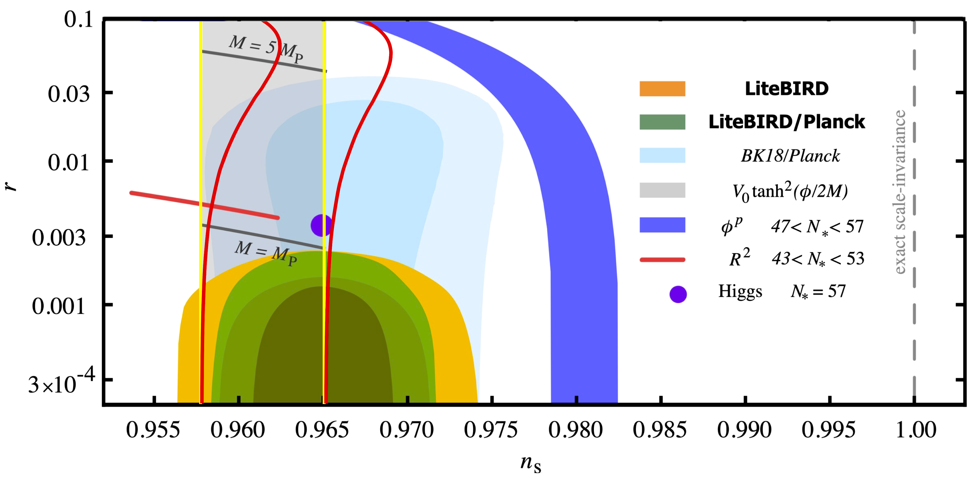
Figure 1: The figure illustrating B-mode targets for LiteBIRD LiteBIRD:2022cnt . The gray area shows the predictions of the simplest $\alpha$-attractor T-models with the potential $V\sim\tanh^{2}{\varphi\over\sqrt{6\alpha}}$. It is surrounded by two yellow lines corresponding to the number of e-foldings $N_{e}=47,57$. We added two red lines for $N_{e}=47,57$ surrounding predictions of E-models of $\alpha$-attractors with the potential $V\sim\big{(}1-e^{-\sqrt{{2\over 3\alpha}}\varphi}\big{)}^{2}$ Kallosh:2013yoa . Predictions of these models cover the left half of the blue area favored by BICEPKeck:2021gln . However, this LiteBIRD figure from LiteBIRD:2022cnt does not contain any targets corresponding to the right part of the blue area.

Kinetic terms in E-models are based on the $SL(2,\mathbb{R})$ symmetry, and T-models have the $SU(1,1)$ symmetry. These symmetries of kinetic terms are slightly broken by the potentials; the main predictions of these models are determined by kinetic terms. A small difference between the predictions of E- and T-models before they reach the attractor point is due to a slightly different way of breaking of these symmetries by the potentials. All of these models have plateau potentials which exponentially fast reach the plateau at large values of the inflaton field,

$$V=V_{0}(1-e^{-\varphi/\mu}+...)\ .$$ (3)

We will call these models ‘exponential $\alpha$-attractors’.

After looking at Fig. 1, one may wonder whether there are any interesting models describing the right part of the area favored by Planck/BICEP/Keck. An interesting example of the models of this type is provided by the KKLTI attractors. Some of these described in Kallosh:2018zsi ; Kallosh:2019hzo have interpretation in terms of Dp-brane inflation Dvali:1998pa ; Dvali:2001fw ; Burgess:2001fx ; Kachru:2003sx ; Lorenz:2007ze ; Martin:2013tda ; Kallosh:2018zsi , though there are other ways to obtain and interpret similar potentials Stewart:1994pt ; Fairbairn:2003yx ; Dong:2010in ; Dimopoulos:2016zhy . In particular, a broad family of such potentials have an interpretation in terms of pole inflation Galante:2014ifa ; Terada:2016nqg ; Karamitsos:2019vor ; Kallosh:2019hzo ; Kallosh:2021mnu , where these potentials appear as attractors. Such attractors have potentials reaching the plateau more slowly, not exponentially but as inverse powers of the inflaton field,

$$V\sim V_{0}(1-{\mu^{k}\over\varphi^{k}}+...)$$ (4)

where $k$ can be any (integer or not) positive constant.

We will call these models ‘polynomial attractors.’ Importantly, cosmological predictions of such models in the large field limit do not depend on the detailed structure of the potential. In particular, the spectral index $n_{s}$ depends only on $k$ Kallosh:2018zsi :

$$n_{s}=1-{2\over N_{e}}{k+1\over k+2}\ .\ .$$ (5)

Thus, investigation of any model with a potential having this behavior at large $\varphi$ gives predictions that are valid for a broad class of the models of this type. That is why they are called attractors. Note that for any $k>0$ the value of $n_{s}$ is greater than the universal prediction of the exponential $\alpha$-attractors $n_{s}=1-{2/N_{e}}\sim 0.964$ for $N_{e}\sim 55$. In the small $k$ limit, the value of $n_{s}$ for these models can reach $1-{1/N_{e}}\sim 0.98$. For small $\mu$, these models can describe any small values of $r$, all the way down to $r=0$. That is why the predictions of this class of inflationary models completely cover the right-hand side of the sweet spot of the Planck/BICEP/Keck data Kallosh:2019hzo ; Kallosh:2018zsi ; Kallosh:2019eeu .

This is illustrated by Fig. 2. The band between the two yellow lines corresponding to $N_{e}=50$ and $60$ is described by the simplest T-model with $V\sim\tanh^{2}{\varphi\over 6\alpha}$, the two red lines correspond to E-models with $V\sim(1-e^{-\sqrt{2\over 3\alpha}\varphi})^{2}$, the purple lines correspond to the KKLTI model with $V\sim{\varphi^{4}\over\varphi^{4}+\mu^{4}}$, and the orange lines describe the model with $V\sim{\varphi^{2}\over\varphi^{2}+\mu^{2}}$.

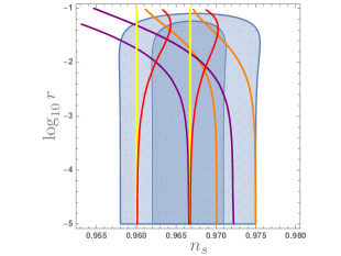
Figure 2: Predictions of the simplest exponential $\alpha$-attractors and KKLTI models superimposed with the Planck2018 constraints on $n_{s}$ and $r$. The band between the two yellow lines is described by the simplest T-model, the two red lines correspond to the simplest E-model. The purple lines correspond to the quartic KKLTI model, and the orange lines describe the quadratic KKLTI model. All bands shown here correspond to $N_{e}$ from 50 to 60.

As explained in Kallosh:2018zsi ; Kallosh:2021mnu , all of these models belong to the general class of pole inflation Galante:2014ifa ; Kallosh:2018zsi . The E- and T- models of $\alpha$-attractors have a pole in the kinetic term of order $q=2$, which is the consequence of the $SL(2,\mathbb{R})$ or $SU(1,1)$ symmetry of the kinetic terms. They have clear geometric origin corresponding to the metric, respectively,

$$ds^{2}=-3\alpha{dTd\bar{T}\over(T+\bar{T})^{2}}\ ,\qquad ds^{2}=-3\alpha{dZd\bar{Z}\over(1-Z\bar{Z})^{2}}\,,\qquad T={1+Z\over 1-Z}\ .$$ (6)

Such kinetic terms often appear in supergravity and string theory.

In comparison, the quartic KKLTI attractors have a pole of order $q=5/2$, and the quadratic ones have $q=3$. Unlike $\alpha$-attractors, pole inflation models with $q\not=2$ are not associated with any known symmetry and do not originate from supergravity, though the corresponding inflaton potentials can be embedded in supergravity Kallosh:2018zsi .

In this paper, we will make yet another step towards unification of all attractors. We will show that it is possible to incorporate the KKLTI models with $V\sim{\varphi^{k}\over\varphi^{k}+\mu^{k}}$ in the context of $\alpha$-attractors in the framework of hyperbolic geometry based on $SL(2,\mathbb{R})$ symmetry or $SU(1,1)$ symmetry of the kinetic terms (6). In order to do it, it was necessary to consider models where the potentials of the $\alpha$-attractors had a singular first derivative at the boundary of the hyperbolic space.

We show that the same potentials in canonical variables are not singular. They have plateau potentials reaching the plateau as inverse powers of the inflaton field, as shown in (4). The cosmological predictions of these models are stable with respect to the significant changes of the original potentials. In particular, their attractor predictions for $n_{s}$ are given by (5). We will also present a unified supergravity model for the exponential and polynomial $\alpha$-attractors.

This means that now the models of such type appear in three independent contexts: as D-brane models, as models of pole inflation with $q>2$, and, finally, as a new family of $\alpha$-attractors. Therefore we believe that these models provide very interesting targets for the future B-mode searches. A combination of the more traditional exponential $\alpha$-attractors Kallosh:2013hoa ; Ferrara:2013rsa ; Kallosh:2013yoa with the polynomial $\alpha$ attractors to be constructed in this paper completely covers the blue area favored by the Plank/BICEP/Keck data shown in Fig. 1.

2 Exponential and polynomial $\alpha$-attractors

2.1 Half-plane variables

There are many different ways to introduce $\alpha$-attractors. In the context of this paper, it is useful to start with the pole interpretation of E-models Galante:2014ifa assuming that the axions of the hyperbolic geometry are fixed and we can study a one-field model

$${\cal L}=-{3\alpha\over 4}{(\partial\rho)^{2}\over\rho^{2}}-V(\rho)\ .$$ (7)

As an example, one may consider a simplest potential which is positive everywhere and regular at $\rho=0$,

$$V=V_{0}(1-b\rho+\ldots)^{2},\qquad b>0\ .$$ (8)

In this expression $\ldots$ represent higher terms in $\rho$. Now we represent this theory in terms of the canonical field $\varphi$, which is related to $\rho$ as follows:

$$\rho=\rho_{0}\,e^{-\sqrt{2\over 3\alpha}\varphi}.$$ (9)

Note that both constants $b$ and $\rho_{0}$ can be absorbed into a redefinition (shift) of the field $\varphi$. Therefore without any loss of generality, the theory (7) can be represented as

$${\cal L}=-{1\over 2}(\partial\varphi)^{2}-V_{0}\Bigl{(}1-e^{-\sqrt{2\over 3\alpha}\varphi}+\ldots\Bigr{)}^{2}.$$ (10)

We called these models E-models, because of the exponential change of variables $\rho=e^{-\sqrt{2\over 3\alpha}\varphi}$. The main stage of inflation occurs at large positive values of the canonically normalized field $\varphi\gg\sqrt{\alpha}$, where the omitted higher order terms are exponentially suppressed, and the potential reduces to

$$V=V_{0}\bigl{(}1-e^{-\sqrt{2\over 3\alpha}\varphi}\bigr{)}^{2}\ .$$ (11)

For $\alpha=1$, this potential coincides with the potential of the Starobinsky model. For small $\alpha$, the cosmological predictions of $\alpha$-attractors are

$$n_{s}=1-{2\over N_{e}}\ ,\qquad r={12\alpha\over N^{2}_{e}}\ .$$ (12)

Note that these two results, in the large $N_{e}$ (or small $\alpha$) limit, do not depend on the detailed structure of $V(\rho)$. Our main assumption was that the potential is a relatively simple function that can be expanded in Taylor series at $\rho=0$.

Once this restriction is removed, the situation may change. For example, if potential $V(\rho)$ is singular at the boundary, the inflaton potential may change dramatically, unless the corresponding corrections are strongly suppressed. In general, it may be possible to use these models constructively. In particular, such models may simplify the solution of the problem of initial conditions for inflation Linde:2017pwt ; Linde:2018hmx . Other applications of such models have been considered for example in Garcia-Saenz:2018ifx ; Iacconi:2021ltm . We will not study models with a singular potential here, but instead we will make one relatively small step: We will consider models where the potential is non-singular, but its derivative is singular. This means that $b=V^{\prime}(\rho)\rightarrow\infty$ near the boundary $\rho\rightarrow 0$. Such modifications preserve the plateau shape of the potential, but may have other important consequences.

As a simplest example, let us add a term $\sim\sqrt{\rho}$ to the potential $V(\rho)$ (8):

$$V=V_{0}(1-a\sqrt{\rho}-b\rho+\ldots)^{2}\ .$$ (13)

This potential is non-singular at small $\rho$, but its derivative is singular. In canonical variables we have

$$V=V_{0}(1-ae^{-\sqrt{1\over 3\alpha}\varphi}-be^{-\sqrt{2\over 3\alpha}\varphi}+\ldots)^{2}.$$ (14)

At large $\varphi$ (after the shift of $\varphi$ absorbing $a$), we have

$$V=V_{0}(1-e^{-\sqrt{1\over 3\alpha}\varphi})^{2}\ .$$ (15)

Thus once again we have the E-model similar to (11), but its effective $\alpha$ doubled. This case shows that the removal of restriction of Taylor series at $\rho=0$ changes the predictions. In this particular case, $n_{s}$ remains the same, we still have a model in a class of the exponential $\alpha$-attractors, but the value of $r$ will be $24\alpha/N^{2}_{e}$, two times greater than in (12).

Note, that this model is still a cosmological attractor. In fact, it is a stronger attractor than the model (8), because the predictions of the new model will not change not only if we add there any terms $O(\rho^{2})$, but also if we add to it any terms $O(\rho)$, which are much greater than $O(\rho^{2})$ in the important limit $\rho\to 0$ corresponding to $\varphi\to\infty$.

Now we will make the next step and consider the logarithmic potential

$$V=V_{0}\,{\ln^{2}\rho\over\ln^{2}\rho+c^{2}}\ .$$ (16)

As before, this potential is finite at $\rho\to 0$, even though its derivative diverges there. In canonical variables, it is given by

$$V=V_{0}\,{\varphi^{2}\over\varphi^{2}+\mu^{2}}\ .$$ (17)

where

$$\mu=\sqrt{3\alpha\,\over 2}c\ .$$ (18)

This potential has a plateau of height $V_{0}$. It is a legitimate $\alpha$-attractor, in more ways than one, although it is different from the exponential $\alpha$-attractors. First of all, the behavior of (17) in the large $\varphi$ limit does not change if we add any terms $\rho^{\nu}$ with $\nu>0$ to the potential (16), or to the denominator or nominator in (16). Secondly, the parameter $\mu^{2}$ vanishes in the limit $\alpha\to 0$. The potential at large $\varphi$ approaches the plateau as

$$V=V_{0}\Big{(}1-{\mu^{2}\over\varphi^{2}}+\dots\Big{)}=V_{0}\Big{(}1-{3\alpha c^{2}\over 2\varphi^{2}}+\dots\Big{)}\ .$$ (19)

Thus, in the new attractors the plateau is described by inverse powers of $\varphi$. For brevity, we called these attractors polynomial to distinguish them from the previously known attractors, where the approach to a plateau was exponentially fast (15).

At small $\mu$, the parameters $n_{s}$ and $r$ reach their attractor values Martin:2013tda ; Kallosh:2018zsi ; Kallosh:2019hzo

$$n_{s}=1-{3\over 2N_{e}},\qquad r={\sqrt{2}\mu\over N_{e}^{3/2}}={\sqrt{3\alpha}\,c\over N_{e}^{3/2}}\ .$$ (20)

The next case to be considered here is

$$V=V_{0}\,{\ln^{4}\rho\over\ln^{4}\rho+c^{4}}\ .$$ (21)

The potential is finite at $\varphi\to 0$, even though its derivative diverges there. In canonical variables, this potential is given by

$$V=V_{0}\,{\varphi^{4}\over\varphi^{4}+\mu^{4}}\,,$$ (22)

where $\mu=\sqrt{3\alpha\,\over 2}c.$ This potential has a plateau of height $V_{0}$. The potential at large $\varphi$ approaches the plateau as $V_{0}\Big{(}1-{\mu^{4}\over\varphi^{4}}+\dots\Big{)}$. At small $\alpha$, the parameters $n_{s}$ and $r$ reach their attractor values Kachru:2003sx ; Martin:2013tda ; Kallosh:2018zsi ; Kallosh:2019hzo

$$n_{s}=1-{5\over 3N_{e}},\qquad r={4\mu^{4/3}\over(3N_{e})^{5/3}}={(4\alpha c^{2})^{{2/3}}\over 3N_{e}^{5/3}}\ .$$ (23)

Similarly, one may consider potentials

$$V=V_{0}\,{\ln^{2n}\rho\over\ln^{2n}\rho+c^{2n}}\ .$$ (24)

In canonical variables, this potential is given by

$$V=V_{0}\,{\varphi^{2n}\over\varphi^{2n}+\mu^{2n}}\,.$$ (25)

One may also consider another class of potentials,

$$V=V_{0}\,{(\ln^{2}\rho+c^{2})^{k/2}-c^{k}\over(\ln^{2}\rho+c^{2})^{k/2}+c^{k}}\ ,$$ (26)

where $k$ and $c$ are any positive numbers. In canonical variables, this potential becomes

$$V=V_{0}\,{(\varphi^{2}+\mu^{2})^{k/2}-\mu^{k}\over(\varphi^{2}+\mu^{2})^{k/2}+\mu^{k}}\ ,$$ (27)

where, as before, $\mu=\sqrt{3\alpha\,\over 2}c$. At large $\varphi$, the potential and its predictions for $n_{s}$ are given by (4), (5):

$$V\sim V_{0}(1-{\mu^{k}\over\varphi^{k}}+...)\ ,\qquad n_{s}=1-{2\over N_{e}}{k+1\over k+2}\ .$$ (28)

Note that for any $k>0$ the attractor values of $n_{s}$ in (28) are greater than $1-2/N_{e}$, and in the limit $k\to 0$ one has $n_{s}\to 1-1/N_{e}$.

2.2 Disk variables

Note that the kinetic term in eq. (7) originates from the hyperbolic geometry in half-plane variables

$$ds^{2}=-3\alpha{dTd\bar{T}\over(T+\bar{T})^{2}}\ .$$ (29)

In Poincaré disk variables the geometry is

$$ds^{2}=-3\alpha{dZd\bar{Z}\over(1-Z\bar{Z})^{2}}\ .$$ (30)

The Cayley transform from half-plane to disk variables, in our approximation that the axions in hyperbolic geometry are stabilized, can be taken in the form

$$\rho={1+z\over 1-z}\ ,$$ (31)

where $z=\tanh{\varphi\over\sqrt{6\alpha}}$. In such case the potentials for polynomial $\alpha$-attractors in disk coordinates are

$$V=V_{0}\,{\ln^{2n}{1+z\over 1-z}\over\ln^{2n}{1+z\over 1-z}+c^{2n}}\ .$$ (32)

The canonical potentials are the same as in equation (25). Similarly, one can use disk variables to describe the broad class of potentials of the type of (27), (28).

3 Supergravity version of exponential and polynomial $\alpha$-attractors

In the previous section, we outlined the embedding of exponential and polynomial $\alpha$-attractors in hyperbolic geometry. Here we present the supergravity version of both types of models using the construction proposed in Kallosh:2017wnt , which we called the Model Building Paradise. It was further developed in Gunaydin:2020ric ; Kallosh:2021vcf . A concise description of the method with various illustrative examples for the case of one inflaton multiplet ($T$ for half-plane case and $Z$ for disk case) and a nilpotent one $X$ with $X^{2}=0$ can be found in Kallosh:2021fvz .

For models in half-plane variables $T$ with stabilized axions one can take the following Kähler potential and superpotential

$$K(T,\overline{T})=-3\alpha\log(T+\overline{T})+{F_{X}^{2}\over F_{X}^{2}+V_{\rm infl}(T,\overline{T})}X\overline{X}\ ,\quad W=(W_{0}+F_{X}X)(2T)^{3\alpha/2}\ ,$$ (33)

which yields

$$V_{\rm total}(Z)=\Lambda+V_{\rm infl}(T,\overline{T})_{|_{T=\overline{T}=t}}\,,\qquad\Lambda=F_{X}^{2}-3W_{0}^{2}\,,\qquad t={T+\overline{T}\over 2}=e^{-\sqrt{2\over 3\alpha}\varphi}\ .$$ (34)

For $V_{\rm infl}(T,\bar{T})=m^{2}(1-T)(1-\bar{T})$ we find the simplest E-model of $\alpha$-attractors with the potential $V_{\rm total}(\varphi)=\Lambda+m^{2}\bigl{(}1-e^{-\sqrt{2\over 3\alpha}\phi}\bigr{)}^{2}$.

For $V_{\rm infl}(T,\overline{T})=V_{0}{\ln^{2n}t\over c^{2n}+\ln^{2n}t}$ one finds a family of polynomial $\alpha$-attractors with the potential $V(\varphi)=\Lambda+V_{0}{\varphi^{2n}\over\mu^{2n}+\varphi^{2n}}$. This is the same potential as in (25), but now it includes an arbitrary cosmological constant $\Lambda$.

For models in disk variables $Z$ we take

$$K(Z,\overline{Z})=-3\alpha\log(1-Z\overline{Z})+{F_{X}^{2}\over F_{X}^{2}+V_{\rm infl}(Z,\overline{Z})}X\overline{X},\quad W=(W_{0}+F_{X}X)(1-Z^{2})^{3\alpha/2}\ ,$$ (35)

which yields

$$V_{\rm total}(Z)=\Lambda+V_{\rm infl}(Z,\overline{Z})_{|_{Z=\overline{Z}=z}}\,,\qquad\Lambda=F_{X}^{2}-3W_{0}^{2}\,,\qquad z^{2}=Z\overline{Z}=\tanh^{2}{\varphi\over\sqrt{6\alpha}}\ .$$ (36)

For $V_{\rm infl}(Z,\overline{Z})=m^{2}z^{2}$, this leads to the simplest T-models of exponential $\alpha$-attractors with $V(\varphi)=\Lambda+m^{2}\tanh^{2}{\varphi\over\sqrt{6\alpha}}$.

For $V_{\rm infl}(Z,\overline{Z})_{|_{Z=\overline{Z}=z}}=V_{0}{\ln^{2n}[{1+z\over 1-z}]\over c^{2n}+\ln^{2n}[{1+z\over 1-z}]}$ this leads, once again, to the family of polynomial $\alpha$-attractors with the potential $V(\varphi)=\Lambda+V_{0}{\varphi^{2n}\over\mu^{2n}+\varphi^{2n}}.$

4 Discussion

As we already mentioned in the Introduction, there are two main types of inflationary models with plateau potentials. The potentials which appear in the Starobinsky model, GL model, Higgs inflation, and in T- and E- models of $\alpha$-attractors have the same basic structure at large positive $\varphi$ shown in (3): Their deviation from the plateau decreases exponentially fast at large $\varphi$. We called such models exponential attractors.

These models are well known and well explored. Their predictions are stable with respect to significant modifications of the models. In particular, all of these models, independently of their physical origin and interpretation, have the same attractor prediction $n_{s}=1-2/N_{s}$ in the large $N_{e}$ limit, consistent with the Planck/BICEP/Keck results. In addition, T- and E- models of $\alpha$ attractors can describe any small values of $r$, and can be formulated in the theories with hyperbolic geometry, which is often encountered in supergravity and string theory. Advanced versions of $\alpha$ attractors have 7 different targets for $r$ in the most interesting range $10^{-3}<r<10^{-2}$.

The second class of attractors with plateau potentials have the potentials reaching the plateau more slowly, like $V_{0}(1-{\mu^{k}/\varphi^{k}})$ (4). We called these models ‘polynomial attractors.’ Cosmological predictions of such models in the large field limit also do not depend on the detailed structure of the potential. In particular, the spectral index $n_{s}$ depends only on $k$ Kallosh:2018zsi .

Some of these models are called KKLTI; they may be related to Dp-brane inflation Dvali:1998pa ; Kachru:2003sx ; Martin:2013tda . A broad class of such models can be incorporated in the general theory of pole inflation with the pole of the kinetic term of degree $q>2$ Galante:2014ifa ; Kallosh:2018zsi . However, until now we did not know whether it is possible to develop these models even further and make them a part of the broad family of $\alpha$-attractors.

In this paper we analyzed this issue and found a large class of polynomial $\alpha$-attractors. The technical reason why they are different from the exponential $\alpha$-attractors has to do with the properties of the potentials and their derivatives near the boundary of the Poincaré disk, as explained in Sec. 2.

These potentials include, in particular, the potentials of the type of ${\varphi^{2n}\over\varphi^{2n}+\mu^{2n}}$ with $\mu^{2}={3\alpha\over 2}c^{2}$. As a result, now such models have three different, independent interpretations. They appear in the context of Dp-brane inflation, and in the context of pole inflation, and now they also belong to a special class of $\alpha$-attractors. Therefore we believe that these models provide very interesting targets for the future B-mode searches.

To explain the phenomenological implications of these results, we added the two simplest polynomial $\alpha$-attractor models (17) and (22) to the LiteBIRD figure Fig. 1 shown in the beginning of this paper. The results are shown in Fig. 3.

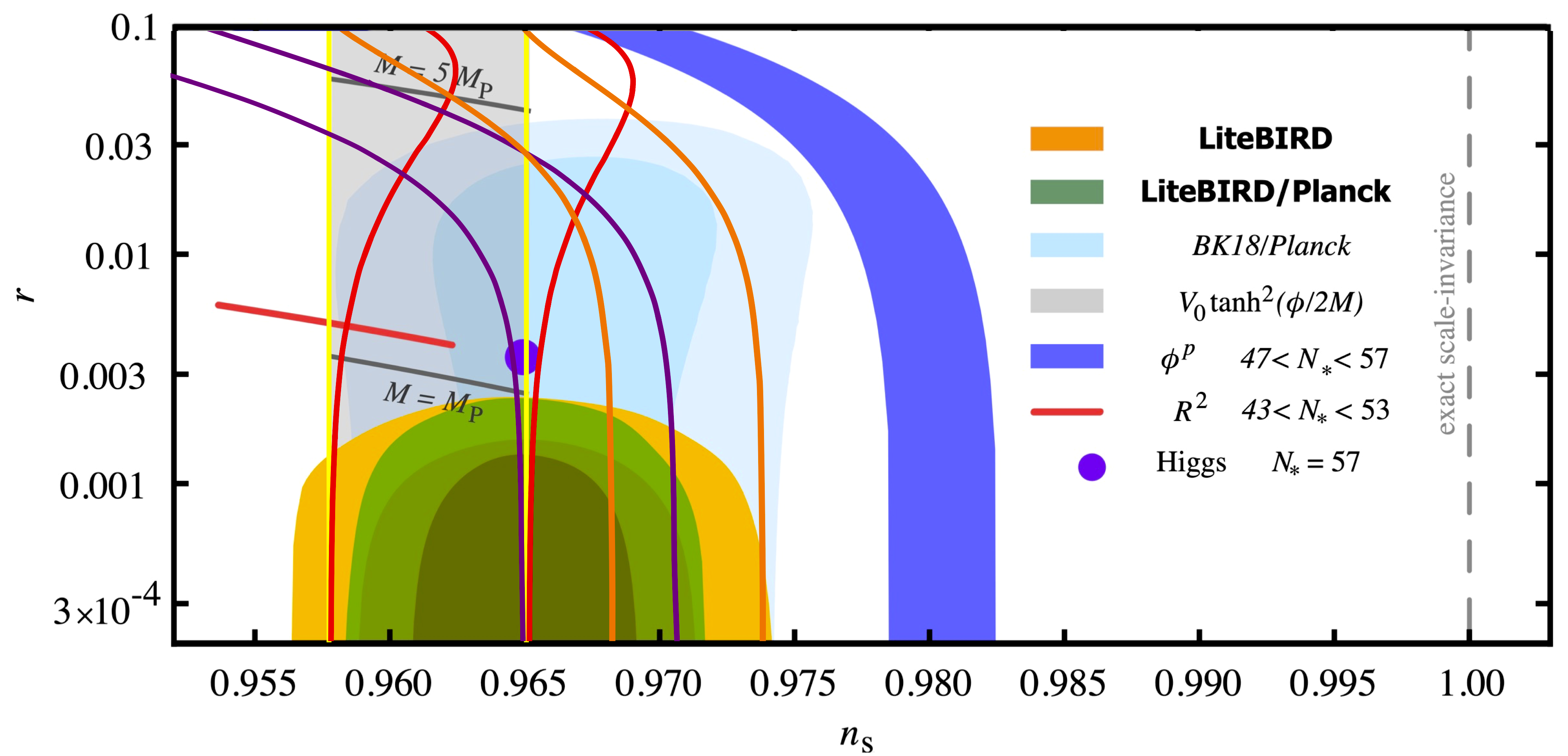
Figure 3: We added predictions of the two simplest polynomial $\alpha$-attractors (17), and (22) to the LiteBIRD figure Fig. 1. As before, the gray area shows the predictions of the simplest $\alpha$-attractor T-models with the potential (1). It is surrounded by two yellow lines corresponding to the number of e-foldings $N_{e}=47,57$. The two red lines for $N_{e}=47,57$ surround the predictions of E-models of $\alpha$-attractors with the potential (2). The purple and orange lines represent the polynomial $\alpha$-attractors ${\varphi^{4}\over\varphi^{4}+\mu^{4}}$ (22), and ${\varphi^{2}\over\varphi^{2}+\mu^{2}}$ (17), for $N_{e}=47$ and 57.

As one can see from Fig. 3, the two simplest T- and E- models (1) and (2) in combination with the two simplest polynomial $\alpha$-attractors (17), and (22) completely cover the dark blue area favored by the latest Planck/BICEP/Keck results.

References

- (1) BICEP/Keck collaboration, Improved Constraints on Primordial Gravitational Waves using Planck, WMAP, and BICEP/Keck Observations through the 2018 Observing Season, Phys. Rev. Lett. 127 (2021) 151301 [2110.00483].
- (2) M. Tristram et al., Improved limits on the tensor-to-scalar ratio using BICEP and Planck, 2112.07961.
- (3) R. Kallosh and A. Linde, BICEP/Keck and cosmological attractors, JCAP 12 (2021) 008 [2110.10902].
- (4) A.A. Starobinsky, A New Type of Isotropic Cosmological Models Without Singularity, Phys. Lett. 91B (1980) 99.
- (5) A.B. Goncharov and A.D. Linde, Chaotic Inflation in Supergravity, Phys. Lett. B139 (1984) 27.
- (6) A.S. Goncharov and A.D. Linde, Chaotic Inflation of the Universe in Supergravity, Sov. Phys. JETP 59 (1984) 930.
- (7) A. Linde, Does the first chaotic inflation model in supergravity provide the best fit to the Planck data?, JCAP 1502 (2015) 030 [1412.7111].
- (8) T. Futamase and K.-i. Maeda, Chaotic Inflationary Scenario in Models Having Nonminimal Coupling With Curvature, Phys. Rev. D 39 (1989) 399.
- (9) D.S. Salopek, J.R. Bond and J.M. Bardeen, Designing Density Fluctuation Spectra in Inflation, Phys. Rev. D40 (1989) 1753.
- (10) F.L. Bezrukov and M. Shaposhnikov, The Standard Model Higgs boson as the inflaton, Phys. Lett. B 659 (2008) 703 [0710.3755].
- (11) R. Kallosh and A. Linde, Universality Class in Conformal Inflation, JCAP 1307 (2013) 002 [1306.5220].
- (12) S. Ferrara, R. Kallosh, A. Linde and M. Porrati, Minimal Supergravity Models of Inflation, Phys. Rev. D88 (2013) 085038 [1307.7696].
- (13) R. Kallosh, A. Linde and D. Roest, Superconformal Inflationary -Attractors, JHEP 11 (2013) 198 [1311.0472].
- (14) M. Galante, R. Kallosh, A. Linde and D. Roest, Unity of Cosmological Inflation Attractors, Phys. Rev. Lett. 114 (2015) 141302 [1412.3797].
- (15) R. Kallosh and A. Linde, Escher in the Sky, Comptes Rendus Physique 16 (2015) 914 [1503.06785].
- (16) R. Kallosh and A. Linde, B-mode Targets, Phys. Lett. B 798 (2019) 134970 [1906.04729].
- (17) R. Kallosh and A. Linde, CMB Targets after PlanckCMB targets after the latest data release, Phys. Rev. D100 (2019) 123523 [1909.04687].
- (18) LiteBIRD collaboration, Probing Cosmic Inflation with the LiteBIRD Cosmic Microwave Background Polarization Survey, 2202.02773.
- (19) S. Ferrara and R. Kallosh, Seven-disk manifold, -attractors, and modes, Phys. Rev. D94 (2016) 126015 [1610.04163].
- (20) R. Kallosh, A. Linde, T. Wrase and Y. Yamada, Maximal Supersymmetry and B-Mode Targets, JHEP 04 (2017) 144 [1704.04829].
- (21) M. Gunaydin, R. Kallosh, A. Linde and Y. Yamada, M-theory Cosmology, Octonions, Error Correcting Codes, JHEP 01 (2021) 160 [2008.01494].
- (22) R. Kallosh, A. Linde, T. Wrase and Y. Yamada, IIB String Theory and Sequestered Inflation, Fortsch. Phys. 69 (2021) 2100127 [2108.08492].
- (23) R. Kallosh, A. Linde and Y. Yamada, Planck 2018 and Brane Inflation Revisited, JHEP 01 (2019) 008 [1811.01023].
- (24) G.R. Dvali and S.H.H. Tye, Brane inflation, Phys. Lett. B 450 (1999) 72 [hep-ph/9812483].
- (25) G.R. Dvali, Q. Shafi and S. Solganik, D-brane inflation, in 4th European Meeting From the Planck Scale to the Electroweak Scale (Planck 2001) La Londe les Maures, Toulon, France, May 11-16, 2001, 2001 [hep-th/0105203].
- (26) C.P. Burgess, M. Majumdar, D. Nolte, F. Quevedo, G. Rajesh and R.-J. Zhang, The Inflationary brane anti-brane universe, JHEP 07 (2001) 047 [hep-th/0105204].
- (27) S. Kachru, R. Kallosh, A.D. Linde, J.M. Maldacena, L.P. McAllister and S.P. Trivedi, Towards inflation in string theory, JCAP 0310 (2003) 013 [hep-th/0308055].
- (28) L. Lorenz, J. Martin and C. Ringeval, Brane inflation and the WMAP data: A Bayesian analysis, JCAP 04 (2008) 001 [0709.3758].
- (29) J. Martin, C. Ringeval and V. Vennin, Encyclopædia Inflationaris, Phys. Dark Univ. 5-6 (2014) 75 [1303.3787].
- (30) E.D. Stewart, Mutated hybrid inflation, Phys. Lett. B 345 (1995) 414 [astro-ph/9407040].
- (31) M. Fairbairn, L. Lopez Honorez and M.H.G. Tytgat, Radion assisted gauge inflation, Phys. Rev. D 67 (2003) 101302 [hep-ph/0302160].
- (32) X. Dong, B. Horn, E. Silverstein and A. Westphal, Simple exercises to flatten your potential, Phys. Rev. D84 (2011) 026011 [1011.4521].
- (33) K. Dimopoulos and C. Owen, Modelling inflation with a power-law approach to the inflationary plateau, Phys. Rev. D 94 (2016) 063518 [1607.02469].
- (34) T. Terada, Generalized Pole Inflation: Hilltop, Natural, and Chaotic Inflationary Attractors, Phys. Lett. B 760 (2016) 674 [1602.07867].
- (35) S. Karamitsos, Beyond the Poles in Attractor Models of Inflation, JCAP 09 (2019) 022 [1903.03707].
- (36) A. Linde, On the problem of initial conditions for inflation, in Black Holes, Gravitational Waves and Spacetime Singularities Rome, Italy, May 9-12, 2017, 2017, http://inspirehep.net/record/1630432/files/arXiv:1710.04278.pdf [1710.04278].
- (37) A. Linde, D.-G. Wang, Y. Welling, Y. Yamada and A. Achucarro, Hypernatural inflation, JCAP 1807 (2018) 035 [1803.09911].
- (38) S. Garcia-Saenz, S. Renaux-Petel and J. Ronayne, Primordial fluctuations and non-Gaussianities in sidetracked inflation, JCAP 07 (2018) 057 [1804.11279].
- (39) L. Iacconi, H. Assadullahi, M. Fasiello and D. Wands, Revisiting small-scale fluctuations in -attractor models of inflation, 2112.05092.
- (40) R. Kallosh, A. Linde, D. Roest and Y. Yamada, induced geometric inflation, JHEP 07 (2017) 057 [1705.09247].
- (41) R. Kallosh, A. Linde, T. Wrase and Y. Yamada, Sequestered Inflation, Fortsch. Phys. 69 (2021) 2100128 [2108.08491].