BiFSMN: Binary Neural Network for Keyword Spotting

Abstract

The deep neural networks, such as the Deep-FSMN, have been widely studied for keyword spotting (KWS) applications. However, computational resources for these networks are significantly constrained since they usually run on-call on edge devices. In this paper, we present BiFSMN, an accurate and extreme-efficient binary neural network for KWS. We first construct a High-frequency Enhancement Distillation scheme for the binarization-aware training, which emphasizes the high-frequency information from the full-precision network’s representation that is more crucial for the optimization of the binarized network. Then, to allow the instant and adaptive accuracy-efficiency trade-offs at runtime, we also propose a Thinnable Binarization Architecture to further liberate the acceleration potential of the binarized network from the topology perspective. Moreover, we implement a Fast Bitwise Computation Kernel for BiFSMN on ARMv8 devices which fully utilizes registers and increases instruction throughput to push the limit of deployment efficiency. Extensive experiments show that BiFSMN outperforms existing binarization methods by convincing margins on various datasets and is even comparable with the full-precision counterpart. We highlight that benefiting from the thinnable architecture and the optimized 1-bit implementation, BiFSMN can achieve an impressive $\mathbf{22.3\times}$ speedup and $\mathbf{15.5\times}$ storage-saving on real-world edge hardware. Our code is released at https://github.com/htqin/BiFSMN.

1 Introduction

With the advent of deep neural networks that process speech, great success has been achieved on speech tasks, such as the Deep Feedforward Sequential Memory Networks (D-FSMN) Zhang et al. (2018). And the deep neural networks for keyword spotting (KWS) are becoming more widely studied for real-world applications on the Internet of Things devices Chen et al. (2014); Zhang et al. (2015); Ren et al. (2020), which enables users to activate devices by speaking keywords or specific phrases, while keeping the device sleeping when inactive. However, such networks are usually deployed on edge devices with limited computation and power while running on-call to wait for any possible speech, which makes the resources for KWS always seriously constrained. To address the challenge, novel algorithms, such as cFSMN Chen et al. (2018), DC-CNN Zhang et al. (2017), and BC-ResNet Kim et al. (2021), have been proposed for efficient deep learning for KWS. Although these works have achieved remarkable speedup and memory footprint reduction, they still rely on expensive floating-point operations.

With the most aggressive bit-width, model binarization Rastegari et al. (2016); Qin et al. (2022) emerges as one of the most promising quantization approaches to compress networks for better computational and storage-usage efficiency. Binary neural networks leverage (1) compact binarized parameters that take limited storage and (2) highly efficient bitwise operations far less costly than their floating-point counterparts. However, although the model binarization community has progressed, binarizing the network for KWS by existing methods is still far from ideal. First, since the application of 1-bit parameters, the representation space of the binarized network is extremely limited and hard to optimize. The direct usage of existing binarization methods severely damages the accuracy of binarized models. Second, existing architectures for KWS have fixed model scales and topologies, which cannot adaptively balance the resource budgets at runtime. Moreover, existing deployment frameworks are far from reaching the theoretical upper limit of acceleration for the binarized network when implemented on real-world hardware.

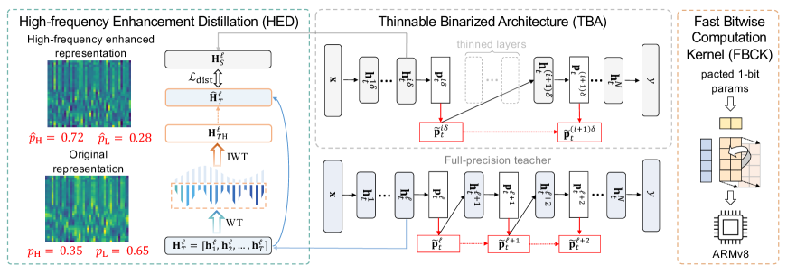
Figure 1: Overview of our BiFSMN, which applies High-frequency Enhancement Distillation (HED) to emphasize significant features and Thinnable Binarized Architecture (TBA) to balance accuracy-efficiency trade-offs, and is implemented by Fast Bitwise Computation Kernel (FBCK) for efficient deployment on real-world devices.

This paper presents a Binarized Feedforward Sequential Memory Network (BiFSMN), which emerges as a successful practice of binary network for KWS application (see the overview in Figure 1), with accurate prediction, lightweight computation, and efficient deployment. BiFSMN is built based on the binarization of D-FSMN, which is a pure feedforward structure. First, we construct a High-frequency Enhancement Distillation (HED) scheme for binarization-aware training, which emphasizes high-frequency information of the full-precision teacher’s representation via wavelet transform that is more crucial for the optimization of the binarized network. Second, to enable adaptive accuracy-efficiency trade-offs at runtime, we propose a Thinnable Binarization Architecture (TBA) to build various depths (such as $[1.0,0.5,0.25]\times$), which further liberates the acceleration potential of the binarized network from the topology perspective to satisfy the different resource constraints. Moreover, we also provide an efficient Fast Bitwise Computation Kernel (FBCK) for BiFSMN on ARMv8 devices. On real-world hardware, the implementation of the BiFSMN using FBCK enjoys impressively faster inference than that using the existing binarization frameworks.

Our BiFSMN is the first binary neural network specialized for KWS. Extensive experiments on Google Speech Commands V1 and V2 datasets (12, 20, and 35 classification tasks) show that our BiFSMN completely outperforms existing binarization methods and is even almost accurate on par with the full-precision counterpart, e.g., BiFSMN just drops within 3% on Speech Commands V1-12. Besides, we highlight that the efficient implementation makes our BiFSMN easy deployment and fast inference in real-world devices: in actual evaluation on edge ARM devices, BiFSMN can achieve up to $22.3\times$ speedup and $15.5\times$ storage-saving compared with the full-precision D-FSMN.

2 Related Work

2.1 Network Binarization

Recently, various binarization methods for neural networks have emerged to compress and accelerate networks. The existing binarization methods are designed to obtain accurate binarized networks by minimizing the quantization error Rastegari et al. (2016), improving loss function Ding et al. (2019), etc. And from the architectures prospective, despite the most popular CNNs Liu et al. (2018), transformer-based and MLP-based networks are also studied for binarization Qin et al. (2021). The practical use of binarization on real devices relies on deployment support. There are binarization frameworks with different target platforms (e.g., CPUs, GPUs, and FPGAs) and applications, such as daBNN Zhang et al. (2019) and Bort Shang et al. (2021).

2.2 Deep Learning for Keyword Spotting

Due to their learning potential and superior performance, deep neural networks for KWS have become widely studied. One classic model is the recurrent neural network (RNN), which enables to capture of the context in a sequence of data Tian et al. (2021). CNN-based (BC-ResNet Kim et al. (2021)) and transform-based (Audiomer) models for KWS are also proposed for better performance and cheaper energy cost. Feedforward Sequential Memory Networks (FSMN) Zhang et al. (2015) mitigates the vanishing gradient problem of RNNs, and is also efficient in computation in convergence. Improvements on the original design of FSMN are varied, such as compact FSMN (cFSMN) Chen et al. (2018), Deep-FSMN (D-FSMN), and pyramidal FSMN (pFSMN) Yang et al. (2018).

3 BiFSMN

In this section, we present the BiFSMN for KWS application. We first build a basic binarization framework and then introduce our techniques, including High-frequency Enhancement Distillation (HED), Thinnable Binarization Architecture (TBA), and Fast Bitwise Computation Kernel (FBCK).

3.1 Basic Binarization Framework

Here we give an introduction to the process of obtaining the basic binarization framework. As one of the most classic and widely used models for speech tasks, D-FSMN Zhang et al. (2018) is considered as a binarization-friendly architecture for the following reasons: (1) The D-FSMN is a pure feedforward structure with the backbone built up by stacking FIR-like memory blocks. (2) D-FSMN introduces skip connections between memory blocks in adjacent layers to allow the information to flow directly to the next layer, which is also proved important for accurate binarized networks Liu et al. (2018). Therefore, we consider the construction of the binarized D-FSMN as the basic binarization framework.

We first introduce the basic formulations of binarization. In the binarized network, both weights and activations are compressed to 1-bit using the $\operatorname{sign}$ function in the forward propagation, and the $\operatorname{STE}$ Courbariaux et al. (2015) is applied to clip the gradient in the backward propagation:

$$\small\operatorname{sign}(x)=\begin{cases}1&\text{if }x\geq 0\\ -1&\text{otherwise }\end{cases},\frac{\partial C}{\partial x}=\begin{cases}\frac{\partial C}{\partial\operatorname{sign}(x)}&\text{if }|x|\leq 1\\ 0&\text{otherwise }\end{cases},$$ (1)

where $C$ is the cost function for the minibatch, $x$ denotes the element in floating-point parameters. The scaling factor $\alpha$ is also introduced to retain the magnitude of real-value weights:

$$\alpha_{\mathbf{w}}=\frac{1}{n}\mathbf{w}^{\top}\mathtt{sign}(\mathbf{w})=\frac{1}{n}\left\|\mathbf{w}\right\|_{l1},$$ (2)

we make $\mathbf{w}\approx\alpha_{\mathbf{w}}\mathbf{B_{w}}$ to reduce the quantization error, where $\mathbf{B_{w}}$ is the 1-bit weight binarized by $\operatorname{sign}$ function.

Then, we introduce the binarized network architecture. When constructing a binarized D-FSMN, we binarize both the floating-point weight and activation for linear and convolutional layers. Given the input $\ell$-th hidden states $\mathbf{H}^{\ell}=[\mathbf{h}_{1}^{\ell},\mathbf{h}_{2}^{\ell},...,\mathbf{h}_{T}^{\ell}]$, and each $\mathbf{h}_{t}^{\ell};t\in[1,T]$ denotes a fixed-size representation of the long surrounding context at time instance $t$. The formulation of the $\ell$-th binarized memory block takes the following form:

$$\tilde{\mathbf{p}}_{t}^{\ell}= \sum_{i=0}^{N_{1}^{\ell}}\alpha_{\mathbf{a}_{i}}^{\ell}\left(\mathbf{B}_{\mathbf{a}_{i}}^{\ell}\otimes\mathbf{B_{p}}_{t-is_{1}}^{\ell}\right)$$ (3)

$$+ \sum_{j=1}^{N_{2}^{\ell}}\alpha_{\mathbf{c}_{j}}^{\ell}\left(\mathbf{B}_{\mathbf{c}_{j}}^{\ell}\otimes\mathbf{B_{p}}_{t+js_{2}}^{\ell}\right)+\mathcal{H}\left(\tilde{\mathbf{p}}_{t}^{\ell-1}\right)+\mathbf{p}_{t}^{\ell}.$$

Here, $\mathbf{p}_{t}^{\ell}=\alpha_{\mathbf{V}}\left(\mathbf{B_{V}}^{\ell}\otimes\mathbf{B_{h}}_{t}^{\ell}\right)+\mathbf{b}^{\ell}$ denotes the linear output of the binarized linear projection layer. $\otimes$ denotes the inner product with bitwise operations XNOR and Bitcount. $\tilde{\mathbf{p}}_{t}^{\ell}$ denotes the output of the memory block. $\mathcal{H}(\cdot)$ denotes the skip connection (identity mapping) within the memory block. $N_{1}^{\ell}$ and $N_{2}^{\ell}$ denotes the look-back and lookahead orders and $s_{1}$ and $s_{2}$ are the stride for look-back and lookahead filters respectively. The input of the units for the next hidden layer $\mathbf{H}^{\ell+1}=[\mathbf{h}_{1}^{\ell+1},\mathbf{h}_{2}^{\ell+1},\cdots,\mathbf{h}_{T}^{\ell+1}]$ is calculated as follow:

$$\mathbf{h}_{t}^{\ell+1}=f\left(\alpha_{\mathbf{U}}^{\ell}\left(\mathbf{B}_{\mathbf{U}}^{\ell}\otimes\tilde{\mathbf{B}}_{\mathbf{p}_{t}}^{\ell}\right)+\mathbf{b}^{\ell+1}\right),$$ (4)

where $f(\cdot)=\operatorname{BN}\cdot\operatorname{Nonlinear}(\cdot)$ denotes the composition of batch normalization and nonlinear functions (PReLU in the binarized network Martinez et al. (2020)).

3.2 High-frequency Enhancement Distillation for Binarization-aware Training

When the neural network is binarized, its representation capability is extremely limited, and the accuracy is significantly decreased compared with the full-precision counterparts. As shown in Figure 2, binarization makes the intermediate representation visually monotonous since it restricts the pixels to binary, while the original feature information is richer and contains much detailed information. However, since it is highly discrete in binarized representations, values on the edges falling to 1 or -1 outline the object, conveying more important information than plain blocks. While it is well-known that edges often present as local maxima of the gradient, which is hard to be improved directly by global optimization.

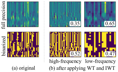
Figure 2: Compared with the original full-precision representation, the relative wavelet energy of the high-frequency component of the binarized representation is larger while that of the low-frequency component is much smaller.

Fortunately, we find that the essence of the information inclination to edge is that the essential binarized representation tends to concentrate on high-frequency components. We use 2D Haar Wavelet Transform (WT) Meyer (1992), which is most frequently used as a separable transform that isolates horizontal and vertical edges, to decompose the representation into low and high-frequency components. The hidden state $\mathbf{H}$ inputted to a specific layer can be represented as a weighted sum of the wavelet function family:

$$f_{\textrm{WT}}(\mathbf{H})=\sum^{-1}_{j=-N}\sum_{k}\mathbf{C}_{j}(k)\phi_{j,k},$$ (5)

where $\phi$ is the mother wavelet function with a specific time parameter, $j=-1,\cdots,-N$ is the resolution level, and $k$ determines the translation of the waveform.

To measure the information amount conveyed by the single component of representation, the relative wavelet energy is used to define the amount of information Rosso et al. (2001). The wavelet energy $E_{j}$ at $j$-th level is first calculated as:

$$E_{j}=\sum_{k}|\mathbf{C}_{j}(k)|^{2}.$$ (6)

When we obtain low and high-frequency coefficients ($\mathbf{C}_{j}\in\{\mathbf{C}_{\textrm{L}},\mathbf{C}_{\textrm{H}}\}$, $N=2$) by once decomposition, their relative wavelet energy $p_{\textrm{H}}$ and $p_{\textrm{L}}$ can be expressed as:

$$p_{\textrm{H}}=\frac{E_{\textrm{H}}}{E_{\textrm{H}}+E_{\textrm{L}}},\qquad p_{\textrm{L}}=\frac{E_{\textrm{L}}}{E_{\textrm{H}}+E_{\textrm{L}}}.$$ (7)

The larger relative wavelet energy demonstrates the information is more gathered in this component. As Figure 2 shows, compared with the full-precision representation, the relative wavelet energy of the high-frequency components of the binarized ones increases significantly, which implies that binarized representation inclines higher-frequency components.

We propose a High-frequency Enhancement Distillation according to the aforementioned analysis. The scheme exploits a full-precision pre-trained D-FSMN model as the teacher to assist the binarization-aware training by enhances the high-frequency components of the full-precision representation in hidden layers. We first apply the wavelet transform on the original hidden states The process can be formulated as follow:

$$\mathbf{H}_{T\textrm{H}}=f_{\textrm{IWT}}\left(\sum_{k}\mathbf{C}_{T\textrm{H}}(k)\phi_{T\textrm{H},k}\right).$$ (8)

And then the emphasized high-frequency representations are added to the original ones:

$$\hat{\mathbf{H}}_{T}=\frac{\mathbf{H}_{T\textrm{H}}}{\sigma(\mathbf{H}_{T\textrm{H}})}+\frac{\mathbf{H}_{T}}{\sigma(\mathbf{H}_{T})},$$ (9)

where $\sigma(\cdot)$ is the standard deviation. Then, inspired by Martinez et al. (2020), we minimize the attention distillation loss between $\hat{\mathbf{H}}_{T}$ from the teacher and $\hat{\mathbf{H}}_{S}$ directly from the hidden states of the student, which is expressed as:

$$\mathcal{L}_{\textrm{dist}}=\sum^{N}_{\ell=1}\left\|\frac{\mathbf{H}^{\ell\ 2}_{S}}{\|\mathbf{H}^{\ell\ 2}_{S}\|}-\frac{\hat{\mathbf{H}}^{\ell\ 2}_{T}}{\|\hat{\mathbf{H}}^{\ell\ 2}_{T}\|}\right\|,$$ (10)

where $\ell$ denotes the $\ell$-th block and $\|\cdot\|$ is the L2-norm.

The HED scheme above makes it easier for the binarized student network to exploit the essential information from emphasized full-precision representations and improve accuracy.

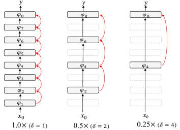
Figure 3: An instance of Thinnable Binarization Architecture ($N=8$, $\delta=1,2,4$) at runtime, where red arrows denote skip connections.

3.3 Thinnable Binarization Architecture for Runtime Accuracy-efficiency Trade-off

As discussed earlier, binarization is an efficient compression approach with extremely lightweight 1-bit parameters and efficient bitwise operations, enabling fast inferences on resource-limited devices. As one of the advantages, binarization will not affect the model architecture, which is critical for well-designed structures. However, the energy budget varies between devices and even during wake-up and power-saving modes on a single device. Therefore, a lightweight yet adaptive binarized architecture, which can switch among different widths at runtime, permits instant and adaptive accuracy-efficiency trade-offs for KWS.

We present a Thinnable Binarization Architecture (TBA) for KWS, which can select a thinner model with fewer layers at runtime, directly reducing the computational consumption. When we focus on the computational expensive backbone, the basic binarization architecture $\textrm{M}^{\prime}$ containing $N$ blocks ($N\in\{2^{n},n\in\mathbf{Z}^{+}\}$) can be expressed as:

$$\textrm{M}^{\prime}(\mathbf{x})=\varphi^{N}\cdot\varphi^{N-1}\cdot...\cdot\varphi^{1}(\mathbf{x}),$$ (11)

where $\textrm{M}^{\prime}$ and $\varphi^{\ell}$ are the binarized network and $\ell$-th binarized D-FSMN block, respectively, and $\mathbf{x}$ is the input of network. The TBA derived from M can be defined as:

$$\textrm{M}(\mathbf{x};\delta)=\Phi^{N}\cdot\Phi^{N-1}\cdot...\cdot\Phi^{1}(\mathbf{x}),$$ (12)

where $\delta$ is the interval of selected layers, which is confined to be divisible into $N$. And each thinnable block $\Phi^{\ell}$ can be defined as

$$\Phi^{\ell}(\mathbf{x})=\begin{cases}\varphi^{\ell}(\mathbf{x}),&\ell\in\{i\delta,i\in[1,N/\delta]\},\\ \mathbf{x},&\textrm{otherwise}.\end{cases}$$ (13)

And the batch normalization in the function $f(\cdot)$ in Eq. (4) in $\ell$-th binarized D-FSMN block $\varphi^{\ell}$ are preassigned according to different variants in the thinnable network. The thinnable network architecture will skip intermediate blocks every $\delta$ layers by replacing them with identity functions. Figure 1 shows the formalization of our thinnable binarization architecture, and we also provide an instance for $N=8$, $\delta=1,2,4$ in Figure 3, which is also the default setting in our experiments.

Input: Fixed pre-trained full-precision teacher $\textrm{M}_{\textrm{FP32}}$ and thinnable binarized model M (BiFSMN) with $N$ basic binarized blocks, training iterations $T$.

Output: Well-trained thinnable binarized model M

for all $t=1,2,\dots,T$ do

       Forward propagate $\textrm{M}_{\textrm{FP}}(\mathbf{x})$ and obtain the information-enhanced intermediate features $\hat{\mathbb{H}}_{T}=\{\hat{\mathbf{H}}_{T}^{1},\hat{\mathbf{H}}_{T}^{2},\dots,\hat{\mathbf{H}}_{T}^{N}\}$;

       for all $\delta=1,2,\dots,\log_{2}N$ do

             Forward propagate $\textrm{M}(\mathbf{x};\delta)$ and obtain the intermediate features $\mathbb{H}_{S}^{\delta}=\{\mathbf{H}_{S}^{\delta},\mathbf{H}_{S}^{2\delta},\dots,\mathbf{H}_{S}^{N}\}$;

             Compute the distillation loss $\mathcal{L}_{\textrm{dist}}^{\delta}$ by Eq. (14);

             Compute the cross-entropy loss $\mathcal{L}_{\textrm{CE}}^{\delta}$;

            

      Descend $\mathcal{L}_{\textrm{tot}}$ as Eq. (15) and update M;

      

Get the well-trained BiFSMN model M;

Evaluate the BiFSMN on test dataset and get the accuracy.

Algorithm 1 The training process of our BiFSMN.

To optimize the binarization-aware training for the proposed TBA, we adopt the uniform layer mapping strategy to better align and learn representation in the HED:

$$\mathcal{L}_{\textrm{dist}}^{\delta}=\sum^{N/\delta}_{i=1}\left\|\frac{\mathbf{H}^{i\delta\ 2}_{S}}{\|\mathbf{H}^{i\delta\ 2}_{S}\|}-\frac{\hat{\mathbf{H}}^{i\delta\ 2}_{T}}{\|\hat{\mathbf{H}}^{i\delta\ 2}_{T}\|}\right\|.$$ (14)

The gradients from different switches are accumulated during backward propagation to update the weight jointly. According to the compression ratio in thinnable architecture, the weighted loss can be calculated as:

$$\mathcal{L}_{\textrm{tot}}=\sum_{\delta}\frac{1}{2^{\delta-1}}\left(\mathcal{L}_{\textrm{CE}}^{\delta}+\gamma\mathcal{L}_{\textrm{dist}}^{\delta}\right),$$ (15)

where $\mathcal{L}_{\textrm{CE}}^{\delta}$ denotes the cross-entropy loss of $\mathrm{M}(\cdot;\delta)$ and $\gamma$ is a hyperparameter to control distillation impact, set to 0.01 as default. The detailed training procedures for the BiFSMN are listed in Algorithm 1.

3.4 Fast Bitwise Computation Kernel for Efficient Hardware Deployment

Benefiting from binarized weights and activations compressed to $\frac{1}{32}$ of the original bit-width, a single binarized layer has an extreme-high $64\times$ theoretical reduction of FLOPs Liu et al. (2018). However, when we implement and deploy the entire binary neural network on real-world hardware using existing binarization deployment frameworks, such as daBNN Zhang et al. (2019) and Bolt huawei noah (2021), its overall inference efficiency is often significantly lower than the theoretical upper limit. One of the key bottlenecks of acceleration is the Binarized General Matrix Multiply (BGEMM) performed with the bitwise XNOR and Bitcount. Therefore, for efficient deployment on edge devices with limited computational resources, we further optimize the 1-bit computation with new instruction and register allocation strategy to accelerate the inference on ARMv8-A architecture widely used on edge devices. We dub it Fast Bitwise Computation Kernel (FBCK).

According to the number of registers on ARMv8 architecture, we first reallocate the registers in the kernel as five partitions in order to improve the register utilization and reduce memory footprint: partition A has four registers (except register v0) for one input (weight/activation), B has two for the other input, C has eight for intermediate results of EOR and CNT, D has eight for the output in one loop, and E has eight for the final results. Each input is packed as INT16. Each register in A stores one input while repeated 8 times, while each in B stores 8 different inputs. We first apply EOR and CNT for A with one register of B to get 32 INT8 results in intermediate partition C, and then perform ADD to accumulate the INT8 to D, and do the same for the other register of B. After sixteen times loop, we finally accumulate the INT8 data stored in D to an INT16 register (in E) using long instruction ADALP, which extends INT8 data to double width. FBCK makes full use of registers almost without idle bits during the computation. Refer to Figure 4 as illustration.

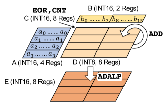
Figure 4: Fast Bitwise Computation Kernel for BiFSMN, which improves the utilization of registers to expand instruction throughput.

4 Experiments

In this section, we conduct experiments on the Google Speech Commands V1 and V2 datasets Warden (2018) to verify the effectiveness of BiFSMN and compare it with state-of-the-art (SOTA) binarization methods and various architectures.

Arch.	Quant	#Bits	FLOPs	V1	V2
D-FSMN	Full Prec.	32/32	710.15	97.51	96.01
D-FSMN	Vanilla	1/1	40.46	87.71	89.53
	Distill	1/1	40.46	90.02	90.95
	HED	1/1	40.46	93.47	93.54
BiFSMN (TBA) [1,0.5,0.25]×	Vanilla	1/1	40.46	87.72	89.96
			29.90	86.95	88.85
			24.62	84.19	87.09
2-6[1pt/1pt]	Distill	1/1	40.46	92.31	93.00
			29.90	91.89	92.84
			24.62	91.83	92.70
2-6[1pt/1pt]	HED	1/1	40.46	95.03	94.86
			29.90	94.87	94.74
			24.62	94.48	94.63

Table 1: Ablation study of BiFSMN on Speech Command 12 tasks. FLOPs denotes million FLOPs, same below.

4.1 Ablation Study

We perform ablation studies to investigate the effect of components of the proposed BiFSMN, including the High-frequency Enhancement Distillation (HED) and Thinnable Binarization Architecture (TBA), on the Speech Commands V1-12 and V2-12 KWS tasks.

As shown in Table  1, the vanilla binarization baseline suffers a significant performance drop in both datasets. The naive distillation scheme helps with the accuracy on the basic D-FSMN architecture, and the application of HED further improves the performance considerably based on distillation. It demonstrates that emphasizing high-frequency information makes it easier for the binarized network to exploit the most crucial representation. And the distillation strategy is also indispensable for better aligning and transferring information.

On the other hand, when solely utilizing TBA, we train a single model but optimize it in different parameter scales through weighted backward propagation. It shows a great deal of potential in not only the adaptive and lightweight computation at runtime but also the optimization of the binarized network during training. Moreover, jointly using HED and TBA further close the accuracy gap between the binarized model and the full-precision counterpart, which is less than 3% on both datasets.

Dataset	Method	#Bits	FLOPs	V1	V2
Speech Commands 12	Full Prec.	32/32	710.15	97.93	98.05
	DoReFa	1/1	40.46	66.42	66.59
	BNN	1/1	35.87	68.84	70.87
	RAD	1/1	35.87	71.51	69.80
	XNOR	1/1	45.04	82.74	87.34
	Bi-Real	1/1	40.46	85.87	87.93
	IR-Net	1/1	40.46	86.81	85.10
	BiFSMN [1,0.5,0.25]×	1/1	40.46	95.03	94.86
			29.90	94.87	94.73
			24.62	94.48	94.63
Speech Commands 20	Full Prec.	32/32	711.20	96.57	97.00
	XNOR	1/1	45.04	80.69	85.05
	Bi-Real	1/1	41.50	80.84	84.39
	IR-Net	1/1	41.50	83.78	83.32
	BiFSMN [1,0.5,0.25]×	1/1	41.50	92.88	92.98
			30.95	92.67	92.81
			25.67	92.65	92.72
Speech Commands 35	Full Prec.	32/32	713.16	96.63	95.96
	IR-Net	1/1	43.47	74.09	74.93
	Bi-Real	1/1	43.47	80.86	81.86
	XNOR	1/1	48.06	81.25	84.05
	BiFSMN [1,0.5,0.25]×	1/1	43.47	92.10	90.67
			32.91	91.93	90.54
			27.63	91.85	90.42

Table 2: Comparison of SOTA binarization methods on Speech Commands V1 and V2 datasets.

4.2 Comparative Experiments

We first compare our BiFSMN with existing structure-independent binarization methods, including BNN Courbariaux et al. (2016), DoReFa Zhou et al. (2016), XNOR Rastegari et al. (2016), Bi-Real Liu et al. (2018), IR-Net Qin et al. (2020), and RAD Ding et al. (2019). We evaluate these binarization methods on 8-block D-FSMN architecture with the same size as the largest variant of BiFSMN. The results in Table 2 show that our 1-bit BiFSMN completely outperforms other SOTA binarization methods by a wide margin. It is noteworthy that BiFSMN even enjoys competitive accuracy to full-precision counterparts within 4% average accuracy drop on both datasets.

Second, to validate the advantage of our TBA from the architecture perspective, we also compare it with various networks widely used in KWS, including FSMN Zhang et al. (2015), VGG19bn Simonyan and Zisserman (2014), BC-ResNet Kim et al. (2021), and Audiomer Sahu et al. (2021). We binarized these architectures with XNOR and IR-Net. In Table 3, our HED can generally be applied in FSMN-based architectures and make a difference for the binarized model performance. Moreover, equipped with TBA, BiFSMN can further strike a balance between accuracy and efficiency at runtime. We further prune the model width and provide an extremely tiny BiFSMN${}_{\textrm{S}}$ (with 32 backbone memory size and 64 hidden size) with only 0.05M parameters and 9.16M FLOPs, demonstrating that our methods also works well on tiny networks.

Arch.	Quant	#Bits	#Param	FLOPs	Acc.
VGG19bn	Full Prec.	32/32	38.97	53348.40	97.74
	IR-Net	1/1	38.97	1030.18	63.86
	XNOR	1/1	38.97	1061.63	66.10
BC-ResNet	Full Prec.	32/32	0.35	3749.71	97.84
	XNOR	1/1	0.35	619.03	65.94
	IR-Net	1/1	0.35	541.70	66.51
Audiomer	Full Prec.	32/32	0.80	18577.49	98.95
	IR-Net	1/1	0.80	1449.41	62.44
	XNOR	1/1	0.80	2567.19	62.44
FSMN	Full Prec.	32/32	0.45	1625.29	97.52
	XNOR	1/1	0.45	80.61	55.89
	IR-Net	1/1	0.45	64.36	88.35
	HED (ours)	1/1	0.45	64.36	89.90
D-FSMN	Full Prec.	32/32	0.60	710.15	97.93
	XNOR	1/1	0.60	45.04	82.74
	IR-Net	1/1	0.60	40.46	86.81
	HED (ours)	1/1	0.60	40.46	93.47
BiFSMN [1,0.5,0.25]×	Full Prec.	32/32	0.60	710.15	97.93
	IR-Net	1/1	0.61	40.46	88.37
				29.90	87.11
				24.62	86.08
2-6[1pt/1pt]	HED (ours)	1/1	0.61	40.46	95.03
				29.90	94.87
				24.62	94.48
BiFSMN [1,0.5,0.25]×	Full Prec.	32/32	0.05	91.62	97.51
	IR-Net	1/1	0.05	11.94	72.21
				10.08	71.70
				9.16	71.66
2-6[1pt/1pt]	HED (ours)	1/1	0.05	11.94	90.65
				10.08	90.33
				9.16	90.31

Table 3: Comparison of various binarized architectures for KWS on Speech Commands V1-12 task. #Param denotes million parameters.

4.3 Deployment Efficiency

To validate the practicability of BiFSMN, we test the actual speed of BiFSMN on Raspberry Pi 3B+ with 1.2GHz 64-bit ARMv8 CPU Cortex-A53.

According to Figure 5, due to the proposed optimized 1-bit Fast Bitwise Computation Kernel, our BiFSMN delivers $10.9\times$ acceleration compared to the full-precision counterparts. It is also much faster than the existing open-source high-performance binarization frameworks (daBNN and Bolt). Furthermore, benefiting from the thinnable architecture, BiFSMN can adaptively balance accuracy and efficiency at runtime according to the resources on device, and switches to BiFSMN_0.5× or BiFSMN_0.25× for further $15.5\times$ and $22.3\times$ speedups, respectively. It shows that our BiFSMN can satisfy different resource constraints.

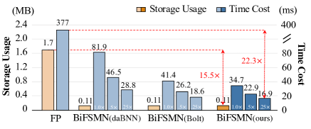
Figure 5: Performance evaluation on real-world ARMv8 devices.

5 Conclusion

We present BiFSMN, an accurate and extreme-efficient binary neural network for KWS. We first construct an HED scheme to emphasize high-frequency information to optimize the training of the binarized network. We also propose a TBA to achieve instant and adaptive accuracy-efficiency trade-offs at runtime. BiFSMN outperforms existing binarization methods by convincing margins and is even comparable to the full-precision counterpart. Moreover, our implementation for BiFSMN on ARMv8 real-world devices achieves an impressive $22.3\times$ speedup and $15.5\times$ storage-saving.

References

- Chen et al. [2014] Guoguo Chen, Carolina Parada, and Georg Heigold. Small-footprint keyword spotting using deep neural networks. In ICASSP, 2014.
- Chen et al. [2018] Mengzhe Chen, Shiliang Zhang, Ming Lei, Yong Liu, Haitao Yao, and Jie Gao. Compact feedforward sequential memory networks for small-footprint keyword spotting. In Interspeech, 2018.
- Courbariaux et al. [2015] Matthieu Courbariaux, Yoshua Bengio, and Jean-Pierre David. Binaryconnect: Training deep neural networks with binary weights during propagations. In NeurIPS, 2015.
- Courbariaux et al. [2016] Matthieu Courbariaux, Itay Hubara, Daniel Soudry, Ran El-Yaniv, and Yoshua Bengio. Binarized neural networks: Training deep neural networks with weights and activations constrained to+ 1 or-1. arXiv, 2016.
- Ding et al. [2019] Ruizhou Ding, Ting-Wu Chin, Zeye Liu, and Diana Marculescu. Regularizing activation distribution for training binarized deep networks. In CVPR, 2019.
- huawei noah [2021] huawei noah. Bolt. https://github.com/huawei-noah/bolt, 2021. Accessed: 2022-01-08.
- Kim et al. [2021] Byeonggeun Kim, Simyung Chang, Jinkyu Lee, and Dooyong Sung. Broadcasted residual learning for efficient keyword spotting. arXiv, 2021.
- Liu et al. [2018] Zechun Liu, Baoyuan Wu, Wenhan Luo, Xin Yang, Wei Liu, and Kwang-Ting Cheng. Bi-real net: Enhancing the performance of 1-bit cnns with improved representational capability and advanced training algorithm. In ECCV, 2018.
- Martinez et al. [2020] Brais Martinez, Jing Yang, Adrian Bulat, and Georgios Tzimiropoulos. Training binary neural networks with real-to-binary convolutions. In ICLR, 2020.
- Meyer [1992] Yves Meyer. Wavelets and Operators: Volume 1. Cambridge university press, 1992.
- Qin et al. [2020] Haotong Qin, Ruihao Gong, Xianglong Liu, Mingzhu Shen, Ziran Wei, Fengwei Yu, and Jingkuan Song. Forward and backward information retention for accurate binary neural networks. In CVPR, 2020.
- Qin et al. [2021] Haotong Qin, Zhongang Cai, Mingyuan Zhang, Yifu Ding, Haiyu Zhao, Shuai Yi, Xianglong Liu, and Hao Su. Bipointnet: Binary neural network for point clouds. In ICLR, 2021.
- Qin et al. [2022] Haotong Qin, Yifu Ding, Mingyuan Zhang, Qinghua YAN, Aishan Liu, Qingqing Dang, Ziwei Liu, and Xianglong Liu. BiBERT: Accurate fully binarized BERT. In ICLR, 2022.
- Rastegari et al. [2016] Mohammad Rastegari, Vicente Ordonez, Joseph Redmon, and Ali Farhadi. Xnor-net: Imagenet classification using binary convolutional neural networks. In ECCV, 2016.
- Ren et al. [2020] Yi Ren, Chenxu Hu, Xu Tan, Tao Qin, Sheng Zhao, Zhou Zhao, and Tie-Yan Liu. Fastspeech 2: Fast and high-quality end-to-end text to speech. In ICLR, 2020.
- Rosso et al. [2001] Osvaldo A Rosso, Susana Blanco, Juliana Yordanova, Vasil Kolev, Alejandra Figliola, Martin Schürmann, and Erol Başar. Wavelet entropy: a new tool for analysis of short duration brain electrical signals. J. Neurosci. Methods, 2001.
- Sahu et al. [2021] Surya Kant Sahu, Sai Mitheran, Juhi Kamdar, and Meet Gandhi. Audiomer: A convolutional transformer for keyword spotting. ArXiv, abs/2109.10252, 2021.
- Shang et al. [2021] Hengchao Shang, Ting Hu, Daimeng Wei, Zongyao Li, Jianfei Feng, Zhengzhe Yu, Jiaxin Guo, Shaojun Li, Lizhi Lei, Shimin Tao, et al. Hw-tsc’s participation in the wmt 2021 efficiency shared task. In Proceedings of the Sixth Conference on Machine Translation, pages 781–786, 2021.
- Simonyan and Zisserman [2014] Karen Simonyan and Andrew Zisserman. Very deep convolutional networks for large-scale image recognition. arXiv:1409.1556, 2014.
- Tian et al. [2021] Yao Tian, Haitao Yao, Meng Cai, Yaming Liu, and Zejun Ma. Improving rnn transducer modeling for small-footprint keyword spotting. In ICASSP, 2021.
- Warden [2018] Pete Warden. Speech commands: A dataset for limited-vocabulary speech recognition. arXiv:1804.03209, 2018.
- Yang et al. [2018] Xuerui Yang, Jiwei Li, and Xi Zhou. A novel pyramidal-fsmn architecture with lattice-free mmi for speech recognition. arXiv:1810.11352, 2018.
- Zhang et al. [2015] Shiliang Zhang, Cong Liu, Hui Jiang, Si Wei, Lirong Dai, and Yu Hu. Feedforward sequential memory networks: A new structure to learn long-term dependency. arXiv:1512.08301, 2015.
- Zhang et al. [2017] Yundong Zhang, Naveen Suda, Liangzhen Lai, and Vikas Chandra. Hello edge: Keyword spotting on microcontrollers. arXiv:1711.07128, 2017.
- Zhang et al. [2018] Shiliang Zhang, Ming Lei, Zhijie Yan, and Lirong Dai. Deep-fsmn for large vocabulary continuous speech recognition. In ICASSP, 2018.
- Zhang et al. [2019] Jianhao Zhang, Yingwei Pan, Ting Yao, He Zhao, and Tao Mei. dabnn: A super fast inference framework for binary neural networks on ARM devices. In ACM MM, 2019.
- Zhou et al. [2016] Shuchang Zhou, Yuxin Wu, Zekun Ni, Xinyu Zhou, He Wen, and Yuheng Zou. Dorefa-net: Training low bitwidth convolutional neural networks with low bitwidth gradients. arXiv, abs/1606.06160, 2016.