Notes on BIM and BFM Optimal Power Flow With Parallel Lines and Total Current Limits

Abstract

The second-order cone relaxation of the branch flow model (BFM) and bus injection model (BIM) variants of optimal power flow are well-known to be equivalent for radial networks. In this work we show that in meshed networks with parallel lines, BIM dominates BFM, and propose novel constraints to make them equivalent in general. Furthermore, we develop an improvement to the second-order cone relaxations of optimal power flow, adding novel and valid linear constraints on the lifted current expressions. We develop two simple test cases to highlight the advantages of the proposed constraints. These novel constraints tighten the second-order cone relaxation gap on test cases in the ‘PG Lib’ optimal power flow benchmark library, albeit generally in limited fashion.

I Introduction

Convex relaxation is a powerful technique to enable global optimization of optimal power flow (OPF). When combined with techniques such as optimality-based bound tightening and cut generation, researchers have been able to prove global optimality of OPF benchmarks of nontrivial size [1, 2, 3]. Generally, one wants very tight (root-node) relaxations, that are minimally expensive to evaluate, and the second-order cone (SOC) relaxations have proven themselves offering exactly this trade-off.

In the context of OPF, there have been two competing frameworks to obtain SOC relaxations: the branch flow model (BFM) and the bus injection model (BIM). The BIM develops expressions using the admittance form of Ohm’s law, allowing all current variables to be eliminated in favour of voltage variables; the BFM still retains a variable for the series current to solve the impedance form of Ohm’s law. The BIM and BFM SOC relaxations were shown to be equivalent for radial networks by Low [4]. Equivalence means the relaxations have the same feasible set, and that we know the bijection.

I-A Different Styles of Branch Models

Generally, authors focus on canonical BIM and BFM relaxations that do not include branch shunt admittance into the branch model (i.e. use a series impedance instead of a $\Pi$-section). We note that from the physics perspective, this just means composing a circuit from series and shunt impedances, and therefore does not introduce any error. Nevertheless, from the perspective of optimization problem feasibility, we need to pay special attention to the bound semantics: the power flow bound applies to the total power flowing into the $\Pi$-section, not just to the power through the series impedance.

Benchmark OPF libraries such as PG Lib [5] use $\Pi$-model branches with an ideal transformer at the sending end (Fig. 1). Coffrin et al. show [6] how to adapt the BIM and BFM SOC relaxations to incorporate shunts and the transformer ratio, and how to correctly apply the apparent power, voltage magnitude, and voltage angle difference bounds.

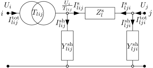
Figure 1: Matpower-style branch model: $\Pi$-section with ideal transformer

Finally, we observe that, Matpower [7], and compatible OPF tools such as PowerModels.jl [8], by default do not use branch current limits, and neither do the benchmarks in PG Lib. Therefore, bounds on the lifted current variables in BFM are generally not included in the problem specification. Nevertheless, if buses have a nonzero lower voltage magnitude bound, it is possible to infer valid current bounds from the known apparent power limits.

I-B Issues With the Relaxations

We demonstrate next that the BIM SOC form is tighter than BFM when there are parallel lines. We therefore include an explicit branch index $l$, to disambiguate parallel lines (i.e. different lines between identical nodes $i$ and $j$). Taking the simple 2-bus system in Fig. 2 as an example, with branch $l$ and $k$ in parallel between buses $i$ and $j$, where branch impedances $Z_{l}$, $Z_{k}$ and the load set point $S_{d}=P_{d}+jQ_{d}$ are known parameters. Voltages on bus $i$ and $j$ are $U_{i},U_{j}$, the complex power flow through branch $l$ in the direction of $i$ to $j$ is $S_{lij}$. We now solve for the generator dispatch value $S_{g}$.

Figure 2: A 2-bus system with parallel lines.

The BIM SOC OPF is formulated as,

$$\operatorname{var} S_{g},W_{i},W_{j},W_{ij},S_{lij},S_{kij},S_{lji},S_{kji},$$ (1a)

$$\min f(\operatorname{Re}(S_{g})),$$ (1b)

$$\operatorname{s.t.} S_{g}=S_{lij}+S_{kij},\quad S_{lji}+S_{kji}=-S_{d},$$ (1c)

$$S_{lij}=Y_{l}^{*}(W_{i}-W_{ij}),\quad S_{kij}=Y_{k}^{*}(W_{i}-W_{ij}),$$ (1d)

$$S_{lji}=Y_{l}^{*}(W_{j}-W_{ij}^{*}),\quad S_{kji}=Y_{k}^{*}(W_{j}-W_{ij}^{*}),$$ (1e)

$$|W_{ij}|^{2}\leq W_{i}W_{j},$$ (1f)

and the BFM as,

$$\operatorname{var} S_{g},W_{i},W_{j},S_{lij},S_{kij},S_{lji},S_{kji},L_{l},L_{k},$$ (2a)

$$\min f(\operatorname{Re}(S_{g})),$$ (2b)

$$\operatorname{s.t.} S_{g}=S_{lij}+S_{kij},\quad S_{lji}+S_{kji}=-S_{d},$$ (2c)

$$S_{lij}+S_{lji}=Z_{l}L_{l},\quad S_{kij}+S_{kji}=Z_{k}L_{k},$$ (2d)

$$|S_{lij}|^{2}\leq W_{i}L_{l},\quad|S_{kij}|^{2}\leq W_{i}L_{k},$$ (2e)

$$W_{j}=W_{i}-Z^{*}_{l}S_{lij}-Z_{l}S^{*}_{lij}+|Z_{l}|^{2}L_{l},$$ (2f)

$$W_{j}=W_{i}-Z^{*}_{k}S_{kij}-Z_{k}S^{*}_{kij}+|Z_{k}|^{2}L_{k}.$$ (2g)

It is noted that these sets have different numbers of independent variables, despite representing the same (nondegenerate) physical system. In the BIM, the bus-pair cross product variable $W_{ij}$ is shared amongst parallel branches between bus $i$ and $j$. Conversely, in the BFM, there is an independent lifted current variable $L_{l}$ for each branch, regardless of whether it is in parallel or not. Therefore, the feasible sets are not equivalent. An ill-informed way to make the BIM and BFM equivalent for parallel lines is to change the BIM formulation with a branch-wise $W_{lij}$ instead of bus-pair-wise $W_{ij}$ variable:

$$\forall lij:W_{lij}\mathrel{\overset{\makebox[0.0pt]{\mbox{\tiny def}}}{=}}U_{i}U_{j}^{*}.$$ (3)

This obviously weakens the BIM relaxation for parallel lines. Existing literature can be interpreted as taking this approach.

Alternatively, we can strengthen the BFM for parallel lines. We can re-write (1d) in terms of $W_{ij}$,

$$W_{ij}=W_{i}-Z^{*}_{l}S_{lij}=W_{i}-Z^{*}_{k}S_{kij},$$ (4)

which implies

$$Z^{*}_{l}S_{lij}=Z^{*}_{k}S_{kij},$$ (5)

is the missing constraint that makes BIM and BFM equivalent again with parallel lines.

We define apparent power branch flow limits on both sides,

$$|S_{lij}|\leq S_{l}^{\text{max}},~{}|S_{lji}|\leq S_{l}^{\text{max}}.$$ (6)

We can now derive bounds on the left-hand side and right-hand side (RHS) of (2e) separately,

$$2S_{l}^{\text{max}}\geq|S_{lij}+S_{lji}|=|Z_{l}L_{l}|\leq Z_{l}\left(\frac{S_{l}^{\text{max}}}{U_{i}^{\text{min}}}\right)^{2}.$$ (7)

The RHS can be significantly tighter in certain situations, for instance ($Z_{l},S_{l}^{\text{max}},U_{i}^{\text{min}}$) = (0.1, 1, 0.9), where the ratio is 162:1. This suggests that implied current bounds can be powerful, and deserve further study.

I-C Scope and Contributions

In this work, we generalize the parallel line consistency constraint (5) for the SOC BFM formulation subject to Matpower-style branch models. Moreover, we propose linear total current limit expressions for both BIM and BFM, and finally study the relaxation gaps numerically.

II BIM & BFM for $\Pi$-sections with Transformer

We now derive the BIM and BFM for Matpower-style $\Pi$-model branches (Fig. 1). Note that this includes an idealized transformer, with complex tap ratio $T_{lij}$, at the sending end of the branch. The power and current bounds now apply at the terminals, not just to the series impedance. Therefore if the shunts are nonzero, the bound semantics are different from the canonical case. We slightly generalize the Matpower branch model to support asymmetric shunts, and conductive shunts. This allows for parameterizing a $\Gamma$-section as an edge case of a $\Pi$-section.

II-A Preliminaries

The shunt at the from-side is $Y^{\text{sh}}_{lij}$, at the to-side $Y^{\text{sh}}_{lji}$; the series impedance is $Z^{\text{s}}_{l}$; the transformer ratio is $T_{lij}$. The current through the series impedance is $I^{\text{s}}_{lij}$ in the direction of $i$ to $j$ and $I^{\text{s}}_{lji}$ for $j$ to $i$. The current through the shunt at the from side is $I^{\text{sh}}_{lij}$ and at the to side is $I^{\text{sh}}_{lji}$. Therefore the current divides over the series and shunt elements as,

$$I^{\text{tot}}_{lij}=(I^{\text{s}}_{lij}+I_{lij}^{\text{sh}})/T^{*}_{lij},\quad I^{\text{tot}}_{lji}=I^{\text{s}}_{lji}+I^{\text{sh}}_{lji},$$ (8)

$$I^{\text{s}}_{lij}+I^{\text{s}}_{lji}=0.$$ (9)

The shunt currents $I_{lij}^{\text{sh}},I_{lji}^{\text{sh}}$ depend on the voltage $U_{i},U_{j}$,

$$I_{lij}^{\text{sh}}=Y^{\text{sh}}_{lij}\frac{U_{i}}{T_{lij}},\quad I_{lji}^{\text{sh}}=Y^{\text{sh}}_{lji}U_{j}.$$ (10)

Ohm’s law between buses $i$ and $j$ through branch $l$ is,

$$U_{j}=\frac{U_{i}}{T_{lij}}-Z^{\text{s}}_{l}I_{lij}^{\text{s}}.$$ (11)

The (total) power flow variables are,

$$S_{lij}^{\text{tot}}\mathrel{\overset{\makebox[0.0pt]{\mbox{\tiny def}}}{=}}U_{i}(I_{lij}^{\text{tot}})^{*},\quad S_{lji}^{\text{tot}}\mathrel{\overset{\makebox[0.0pt]{\mbox{\tiny def}}}{=}}U_{j}(I_{lji}^{\text{tot}})^{*},$$ (12)

and the apparent power limits apply,

$$|S_{lij}^{\text{tot}}|^{2}\leq(S_{l}^{\text{max}})^{2},|S_{lji}^{\text{tot}}|^{2}\leq(S_{l}^{\text{max}})^{2}.$$ (13)

We define the power flow through the series impedance,

$$S_{lij}^{\text{s}}\mathrel{\overset{\makebox[0.0pt]{\mbox{\tiny def}}}{=}}\frac{U_{i}}{T_{lij}}(I_{lij}^{\text{s}})^{*},\quad S_{lji}^{\text{s}}\mathrel{\overset{\makebox[0.0pt]{\mbox{\tiny def}}}{=}}U_{j}(I_{lji}^{\text{s}})^{*}.$$ (14)

Note that the sending end series power flow variable uses ${U_{i}}/{T_{lij}}$ – not $U_{i}$ – as the voltage variable. We can substitute $S_{lij}^{\text{tot}}$ for $S_{lij}^{\text{s}}$, by substituting (8) into (12),

$$S_{lij}^{\text{tot}}=(Y^{\text{sh}}_{lij})^{*}\frac{W_{i}}{|T_{lij}|^{2}}+S_{lij}^{\text{s}},~{}S_{lji}^{\text{tot}}=(Y^{\text{sh}}_{lji})^{*}W_{j}+S_{lji}^{\text{s}}.$$ (15)

The lifted series current variable $L_{l}^{\text{s}}$ is,

$$0\leq L_{l}^{\text{s}}\mathrel{\overset{\makebox[0.0pt]{\mbox{\tiny def}}}{=}}I_{lij}^{\text{s}}(I_{lij}^{\text{s}})^{*}=I_{lji}^{\text{s}}(I_{lji}^{\text{s}})^{*}.$$ (16)

The lifted voltage variable $W_{i}$ is,

$$(U_{i}^{\text{min}})^{2}\leq W_{i}\mathrel{\overset{\makebox[0.0pt]{\mbox{\tiny def}}}{=}}U_{i}U_{i}^{*}\leq(U_{i}^{\text{max}})^{2}.$$ (17)

The lifted voltage cross-product variable $W_{ij}$ is,

$$-U_{i}^{\text{max}}U_{j}^{\text{max}}\leq W_{ij}\mathrel{\overset{\makebox[0.0pt]{\mbox{\tiny def}}}{=}}U_{i}U_{j}^{*}\leq U_{i}^{\text{max}}U_{j}^{\text{max}}.$$ (18)

The angle differences between adjacent buses are constrained through $\theta_{ij}^{\text{max}}$,

$$-\pi/4\leq\theta_{ij}^{\text{min}}\leq\angle U_{i}-\angle U_{j}=\angle U_{i}U_{j}^{*}\leq\theta_{ij}^{\text{max}}\leq\pi/4.\phantom{-}$$ (19)

In terms of $W_{ij}$, this becomes,

$$\tan(\theta_{ij}^{\text{min}})\operatorname{Re}(W_{ij})\leq\operatorname{Im}(W_{ij})\leq\tan(\theta_{ij}^{\text{max}})\operatorname{Re}(W_{ij}).$$ (20)

II-B BFM SOC Formulation

Ohm’s law is obtained by multiplying (11) with its own conjugate, and substituting in the lifted variables,

$$W_{j}=\frac{W_{i}}{|T_{lij}|^{2}}-\left(Z_{l}^{*}S^{\text{s}}_{lij}+\left(Z_{l}^{*}S^{\text{s}}_{lij}\right)^{*}\right)+|Z_{l}|^{2}L^{\text{s}}_{l}.$$ (21)

The SOC constraints are obtained by multiplying (14) with its conjugate, and then relaxing to an inequality,

$$|S_{lij}^{\text{s}}|^{2}\leq\frac{W_{i}}{|T_{lij}|^{2}}L_{l}^{\text{s}}.$$ (22)

We obtain the loss balance by multiplying (11) with $(I^{\text{s}}_{lij})^{*}$

$$S_{lij}^{\text{s}}+S_{lji}^{\text{s}}=Z^{\text{s}}_{l}L^{\text{s}}_{l}.$$ (23)

II-C BIM SOC Formulation

We rewrite Ohm’s law (11) in admittance form

$$I^{\text{s}}_{lij}=Y^{\text{s}}_{l}\left(\frac{U_{i}}{T_{lij}}-U_{j}\right),\quad I^{\text{s}}_{lji}=Y^{\text{s}}_{l}\left(U_{j}-\frac{U_{i}}{T_{lij}}\right).$$ (24)

We take the conjugate of (24) and multiply with $U_{i}/T_{lij},U_{j}$ to obtain,

$$S_{lij}^{\text{s}}=(Y^{\text{s}}_{l})^{*}\left(\frac{W_{i}}{|T_{lij}|^{2}}-\frac{W_{ij}}{T_{lij}}\right),$$ (25)

$$S_{lji}^{\text{s}}=(Y^{\text{s}}_{l})^{*}\left(W_{j}-\frac{W_{ji}}{T_{lij}^{*}}\right).$$ (26)

We get the total flow expressions by substituting the above into (15). The SOC constraint, to link everything together, is,

$$|W_{ij}|^{2}\leq W_{i}W_{j}.$$ (27)

II-D Valid Current Bounds

Given the total power limit $S_{l}^{\text{max}}$, we can derive a valid bound on the series current, at the sending end,

$$|I_{lij}^{\text{tot}}|\leq S_{l}^{\text{max}}/U_{i}^{\text{min}},\quad|I_{lij}^{\text{sh}}|\leq|Y^{\text{sh}}_{lij}|U_{i}^{\text{max}}/|T_{lij}|,$$ (28)

$$\implies|I_{lij}^{\text{s}}|\leq I_{lij}^{\text{s,max}}\mathrel{\overset{\makebox[0.0pt]{\mbox{\tiny def}}}{=}}|T_{lij}||I_{lij}^{\text{tot}}|+|I_{lij}^{\text{sh}}|.$$ (29)

and at the receiving end,

$$|I_{lji}^{\text{tot}}|\leq S_{l}^{\text{max}}/U_{j}^{\text{min}},|I_{lji}^{\text{sh}}|\leq|Y^{\text{sh}}_{lji}|U_{j}^{\text{max}},$$ (30)

$$\implies|I_{lji}^{\text{s}}|\leq I_{lji}^{\text{s,max}}\mathrel{\overset{\makebox[0.0pt]{\mbox{\tiny def}}}{=}}|I_{lji}^{\text{tot}}|+|I_{lji}^{\text{sh}}|.$$ (31)

Finally, using (9) we know $|I_{lij}^{\text{s}}|=|I_{lji}^{\text{s}}|$, and therefore

$$I_{l}^{\text{s,max}}\mathrel{\overset{\makebox[0.0pt]{\mbox{\tiny def}}}{=}}\min(I_{lij}^{\text{s,max}},I_{lji}^{\text{s,max}}),\implies L^{s}_{l}\leq(I_{l}^{\text{s,max}})^{2}.$$ (32a)

We can still enforce a total current limit in this variable space. We substitute (10) into (8),

$$T_{lij}^{*}I^{\text{tot}}_{lij}=\left(I^{\text{s}}_{lij}+Y^{\text{sh}}_{lij}\frac{U_{i}}{T_{lij}}\right),I^{\text{tot}}_{lji}=I^{\text{s}}_{lji}+Y^{\text{sh}}_{lji}U_{j}.$$ (33)

Note that this procedure guarantees that either of the total current limits is binding before the series current.

Now we multiply this expression with its own conjugate and perform the variable substitutions,

$$|T_{lij}|^{2}L^{\text{tot}}_{lij}=L^{\text{s}}_{l}+Y^{\text{sh}}_{lij}S^{\text{s}}_{lij}+(Y^{\text{sh}}_{lij}S^{\text{s}}_{lij})^{*}+|Y^{\text{sh}}_{lij}|^{2}\frac{W_{i}}{|T_{lij}|^{2}}$$

$$\leq|T_{lij}|^{2}\left(\frac{S_{l}^{\text{max}}}{U_{i}^{\text{min}}}\right)^{2}.$$ (34)

Similarly, the receiving end total lifted current variable is,

$$L^{\text{tot}}_{lji}=L^{\text{s}}_{l}+Y^{\text{sh}}_{lji}S^{\text{s}}_{lji}+(Y^{\text{sh}}_{lji}S^{\text{s}}_{lji})^{*}+|Y^{\text{sh}}_{lji}|^{2}{W_{j}}\leq\left(\frac{S_{l}^{\text{max}}}{U_{j}^{\text{min}}}\right)^{2}.$$

(35)

For the BIM SOC model, introducing such constraints is more complicated noting that $L^{s}_{l}$ is not defined in the BIM variable space. Therefore, we introduce linking equalities.

II-E Linking Equalities

Generally, the variable $L_{l}$ is only used in the BFM, and $W_{ij}$ only in BIM. Nevertheless, as the relaxations are incomparable, as discussed in Section I-B, it is useful to intersect them. Therefore we want to 1) derive the $W_{ij}$ variable as an expression of the natural BFM variables 2) derive the $L_{l}$ variable as an expression of the natural BIM variables.

II-E1 BIM expressions in terms of $W_{i},S_{lij}^{\text{s}}$

For the first case, we rewrite (25)-(26),

$$W_{ij}=T_{lij}\frac{W_{i}}{|T_{lij}|^{2}}-(Z^{\text{s}}_{l})^{*}T_{lij}S_{lij}^{\text{s}},$$ (36a)

$$W_{ji}=T_{lij}^{*}W_{j}-(Z^{\text{s}}_{l})^{*}T_{lij}^{*}.S_{lji}^{\text{s}}$$ (36b)

We can now project the known bounds and the 4D cuts [9] on $W_{ij}$ onto $S^{\text{s}}_{lij},L^{\text{s}}_{l}$. The case of the parallel branches still needs to be considered. We consider a case with two parallel branches $(l,i,j)$ and $(k,i,j)$, which must necessarily have identical $W_{ij}$ values, and use (36a) to obtain,

$$T_{lij}\frac{W_{i}}{|T_{lij}|^{2}}-(Z^{\text{s}}_{l})^{*}T_{lij}S_{lij}^{\text{s}}=T_{kij}\frac{W_{i}}{|T_{kij}|^{2}}-(Z^{\text{s}}_{k})^{*}T_{kij}S_{kij}^{\text{s}}.$$

(37)

which generalizes (5) to the Matpower-style branch model. We need such a constraint to link the power flow variables through parallel lines pair-wise in the same way that $W_{ij}$ does.

II-E2 BFM expressions in terms of $W_{i},W_{ij}$

For the second case, we substitute (25)-(26) into (23), and divide by $Z_{l}$,

$$\footnotesize\!\!L^{\text{s}}_{l}=|Y^{\text{s}}_{l}|^{2}\!\!\left(\frac{W_{i}}{|T_{lij}|^{2}}-T_{lij}^{*}\frac{W_{ij}}{|T_{lij}|^{2}}-T_{lij}\frac{W_{ji}}{|T_{lij}|^{2}}+W_{j}\right).$$ (38)

allowing us to place linear bounds on the total current magnitude when combined with (34)-(35).

III Numerical Experiments

We want to compare different formulations, in terms of gap w.r.t. the upper bound AC polar solution, as well as computation time, for:

1. the canonical BIM relaxation used in PG Lib [5] as implemented in PowerModels.jl [8];

2. the improved BFM relaxation with added implied total current limits (32) and parallel lines constraints (37);

3. the improved BIM relaxation with added the total current limits (32).

We use Ipopt [10] as the SOC solver with Mumps as the linear solver.

III-A Feasible Sets

The KCL expression is the same for all variants,

$$\forall i:\sum_{lij\in\mathcal{T}}S^{\text{tot}}_{lij}+\sum_{d\in\mathcal{D}}S_{d}-\sum_{g\in\mathcal{G}}S_{g}=0.$$ (39)

and the generator output lies in a PQ space $\mathcal{S}_{g}$,

$$S_{g}\in\mathcal{S}_{g}.$$ (40)

We minimize the generation cost, using linear and quadratic coefficients $c_{g,1},c_{g,2}$ w.r.t active power output $P_{g}=\operatorname{Re}(S_{g})$,

$$\min\sum_{g\in\mathcal{G}}\left(c_{g,1}P_{g}+c_{g,2}(P_{g})^{2}\right).$$ (41)

III-A1 Shared constraints

• generation cost objective (41);

• complex power flow variables (12) or (14);

• apparent power flow bounds (13);

• lifted voltage variable with bounds (17);

• KCL with constant power loads (39);

• generator output (40);

• shunt power loss in branch (15);

• lifted (4D) nonlinear cuts [6].

III-A2 BIM Canonical

Shared +

• lifted voltage crossproduct variable bounds (18);

• series power flow in branch (25), (26);

• SOC linking constraint (27);

• voltage angle difference constraints (20).

III-A3 BFM Canonical

Shared +

• lifted series current variable (16), (32a)

• series power flow in branch (23);

• SOC linking constraint (22);

• voltage angle difference constraints (20) + (36a);

• linking variable for 4D nonlinear cuts (36a).

III-A4 BIM Improved

BIM Canonical +

• total current bounds (34), (35);

• lifted series current expression (38).

III-A5 BFM Improved

BFM Canonical +

• total current bounds (34), (35);

• parallel lines consistency (37).

III-B Novel Small Test Cases

We propose two simple test cases to highlight the improvements proposed in this article.

III-B1 case2_parallel

In this newly proposed 2-bus test case with 2 lines in parallel (Similar to Fig. 2, but with generator 2 added on bus 2, parameters in Table I). The case is set up to have congestion on line 2. The generator on bus 2 is more expensive than on line 1, so preferably gen 1 would be dispatched. Without the parallel line constraint, it is possible to control the flow through the branches independently, and therefore gen 1 gets dispatched to supply all of the load, i.e. at a value of $P_{g=1}=1.146$. With the parallel line constraint, Kirchhoff’s voltage law is correctly applied, and current is shared appropriately between the branches, and therefore both generators need to be dispatched $P_{g=1}=0.075$, $P_{g=2}=1.040$.

The BIM relaxation is exact (0 gap), matching the value of the ACOPF upper bound at 5.27360. The BFM relaxation however has a gap of 78.264 %, which goes to 0 when adding the parallel line constraints.

TABLE I: Parameters for the 2-bus parallel system, where the units for all parameters are p.u. except for $\Delta\theta_{12}^{\text{min}},\Delta\theta_{12}^{\text{max}}$ (in degree) and $c_{1},c_{0}$, which are generator cost coefficients.

Symbol	Value	Symbol	Value
$Z_{l},Y^{\text{sh}}_{lij},Y^{\text{sh}}_{lji}$	$0.065+j0.62,j0.225,j0.225$	$S_{l}^{\text{max}}$	$90$
$Z_{k},Y^{\text{sh}}_{kij},Y^{\text{sh}}_{kji}$	$0.025-j0.75,j0.35,j0.35$	$S_{k}^{\text{max}}$	$0.5$
$g=2:c_{g,1},c_{g,2}$	5.0, 0.0	$\Delta\theta_{ij}^{\text{min}},\Delta\theta_{ij}^{\text{max}}$	$-30^{\circ},30^{\circ}$
$g\in{1,2}:P_{g}^{\text{min}},P_{g}^{\text{max}}$	$0.0,2.0$	$U_{i}^{\text{min}},U_{i}^{\text{max}}$	$0.90,1.10$
$g\in{1,2}:Q_{g}^{\text{min}},Q_{g}^{\text{max}}$	$-10.0,1.0$	$U_{j}^{\text{min}},U_{j}^{\text{max}}$	$0.90,1.10$
$g=1:c_{g,1},c_{g,2}$	1.0, 0.0	$S_{d}$	$1.1+j0.4$

III-B2 case2_gap

We fine tune a 2-bus 1-branch system to create a significant gap, to demonstrate the effectiveness of the implied constraints on the total current. The circuit is presented in Fig. 3 and parameters are listed in Table II.

Figure 3: The 2-bus system to demonstrate the power of implied current limits.

TABLE II: Parameters for the 2-bus system, where the units for all parameters are p.u. except for $\Delta\theta_{12}^{\text{min}},\Delta\theta_{12}^{\text{max}}$ (in degree) and $c_{1},c_{0}$, which are generator cost coefficients.

Symbol	Value	Symbol	Value
$Z_{l},Y^{\text{sh}}_{lij},Y^{\text{sh}}_{lji},$	$0.065+j0.62,j0.9,j0.9$	$P_{g=2}^{\text{min}},P_{g=2}^{\text{max}}$	$0.0,2.0$
$S_{d=1},S_{d=2}$	$0.11+j0.4,0.9+j0.5$	$Q_{g=2}^{\text{min}},Q_{g=2}^{\text{max}}$	$-1.0,1.0$
$P_{g=1}^{\text{min}},P_{g=1}^{\text{max}}$	$0.0,2.0$	$S_{l}^{\text{max}},I_{l}^{\text{max}}$	$0.80,0.8551$
$Q_{g=1}^{\text{min}},Q_{g=1}^{\text{max}}$	$-1.0,1.0$	$U_{i}^{\text{min}},U_{i}^{\text{max}}$	$0.94,1.10$
$\Delta\theta_{ij}^{\text{min}},\Delta\theta_{ij}^{\text{max}}$	$-30^{\circ},30^{\circ}$	$c_{g,1},c_{g,2}$	g=1: $20,~{}0$ g=2: $-10,~{}0$

For the studied case, the optimal objective value of the nonlinear AC OPF problem is 11.5816. The Canonical BIM SOC model leads to a gap of 105.89 % while the gap for the Improved BIM/BFM formulations with implied total current limit is only 2.92 %. As shown in Table II, the implied bound for the total current is,

$$I_{lij}^{\text{max}}=I_{lji}^{\text{max}}={S_{l}^{\text{max}}}/{U_{i}^{\text{min}}}={S_{l}^{\text{max}}}/{U_{j}^{\text{min}}}=0.8551.$$ (42)

For the Canonical BIM, the optimal total current values at the from and to ends are 4.061 and 4.437, respectively. In the Improved BIM formulation, the total current at both ends of the line are exactly at the limit, i.e., 0.8551. We note that the current limit really puts a lot of pressure on the feasible space of the power flow losses in the individual branches.

III-C PG Lib Results

Table III lists the results of numerical experiments. We focus on a selection of networks where the proposed improvements close the gap significantly, i.e. more than 0.02 %.

TABLE III: PGLib_OPF_ case results. Parentheses indicate Ipopt output status “ALMOST_LOCALLY_SOLVED” instead of “LOCALLY_SOLVED”.

Case	AC-polar [5]	BIM can.		BIM impr.		BFM impr.
	obj ($\$/h$)	t (s)	gap (%)	t (s)	gap (%)	t (s)	gap (%)
39_epri	138415.56	$<1$	0.55	$<1$	0.35	$<1$	0.35
162_ieee_dtc	108075.64	1	5.94	1	4.73	1	4.73
588_sdet	313139.78	3	2.14	4	1.91	3	1.91
1888_rte	1402530.82	201	2.04	198	0.97	23	0.97
4661_sdet	2251344.07	48	1.98	65	1.89	48	1.89
6468_rte	2069730.15	119	1.12	(207)	(0.98)	273	0.98

The authors propose the following interpretation of why the total current limits can tighten the gap, despite not using new information (as it would be to use independent information on ampacity). In the optimal solution of AC OPF, the implied current limits can only be binding when the apparent power limits are binding as well. However due to the relaxation, the bounds on the total current variables can nevertheless be binding before the apparent power bounds are binding.

Focusing now on the broader set of PG Lib test cases, the Improved BIM OPF is slower than the Canonical BIM; whereas Improved BFM and Canonical BIM are very similar in speed. Finally, the Improved BIM and Improved BFM have very similar calculation times (on average BFM 1.7 % faster).

We note that in the implementation, we did not introduce auxiliary variables for the linking equalities §II-E but instead performed the substitutions. This obviously makes the BIM denser than the BFM from the perspective of the total current limits. Further exploration on whether elimination of these variables helps or hurts performance is needed. However, basing the distinction between BIM and BFM on the variable space ($S^{\text{tot}}_{lij},W_{i},W_{ij}$ vs $S^{\text{tot}}_{lij},W_{i},L_{l}$) may then become ambiguous.

IV Conclusions

We propose two novel constraint sets, one for implied total current limits, and one for parallel lines, to strengthen the canonical second-order conic BIM and BFM relaxations for networks with $\Pi$-sections as building blocks. Two test cases are developed that illustrate the difference w.r.t. SOC BIM and BFM relaxations without these novel constraints. We show that, by exploiting implied total current limits (using only apparent power limits and voltage bounds), we can tighten the canonical BIM and BFM relaxations. Due to the relaxation step, it is possible that the implied total current bounds become binding before the original apparent power bounds. The total current limits seem particularly effective when the objective incentivizes network losses, e.g. when generation cost is negative, or dispatching load can solve congestions.

Finally, we note that OPF with current limits (as opposed to apparent power limits) is an under-explored topic, despite thermal loading being a function of power loss, which is a quadratic function of current (magnitude) - not power. The proposed loss bounds can also be used to strengthen network flow relaxations [11].

References

• [1] S. Xu, R. Ma, D. K. Molzahn, H. Hijazi, and C. Josz, “Verifying global optimality of candidate solutions to polynomial optimization problems using a determinant relaxation hierarchy,” 2021. [Online]. Available: http://arxiv.org/abs/2101.00621
• [2] S. Gopinath, H. L. Hijazi, T. Weisser, H. Nagarajan, M. Yetkin, K. Sundar, and R. W. Bent, “Proving global optimality of ACOPF solutions,” Electric Power Syst. Res., vol. 189, no. October 2019, p. 106688, 2020.
• [3] K. Sundar, H. Nagarajan, S. Misra, M. Lu, C. Coffrin, and R. Bent, “Optimization-Based Bound Tightening using a Strengthened QC-Relaxation of the Optimal Power Flow Problem,” 2018. [Online]. Available: http://arxiv.org/abs/1809.04565
• [4] S. H. Low, “Convex relaxation of optimal power flow - part I: formulations and equivalence,” IEEE Trans. Control Netw. Syst., vol. 1, no. 1, pp. 15–27, mar 2014.
• [5] S. Babaeinejadsarookolaee, A. Birchfield, R. D. Christie, C. Coffrin, C. DeMarco, R. Diao, M. Ferris, S. Fliscounakis, S. Greene, R. Huang, C. Josz, R. Korab, B. Lesieutre, J. Maeght, D. K. Molzahn, T. J. Overbye, P. Panciatici, B. Park, J. Snodgrass, and R. Zimmerman, “The power grid library for benchmarking AC optimal power flow algorithms,” [math.OC], pp. 1–17, 2019.
• [6] C. Coffrin, H. L. Hijazi, and P. Van Hentenryck, “DistFlow extensions for AC transmission systems,” [Math.OC], pp. 1–19, 2015.
• [7] R. D. Zimmerman, C. E. Murillo-Sánchez, and R. J. Thomas, “MATPOWER: steady-state operations, systems research and education,” IEEE Trans. Power Syst., vol. 26, no. 1, pp. 12–19, 2011.
• [8] C. Coffrin, R. Bent, K. Sundar, Y. Ng, and M. Lubin, “PowerModels.jl: an open-source framework for exploring power flow formulations,” in Power Syst. Comp. Conf., vol. 20, Dublin, Ireland, 2018, p. 8.
• [9] C. Coffrin, H. Hijazi, and P. Van Hentenryck, “Strengthening the SDP relaxation of ac power flows with convex envelopes, bound tightening, and valid inequalities,” IEEE Trans. Power Syst., vol. 32, no. 5, pp. 3549–3558, 2017.
• [10] A. Wächter and L. T. Biegler, “On the implementation of primal-dual interior point filter line search algorithm for large-scale nonlinear programming,” Math. Prog., vol. 106, no. 1, pp. 25–57, 2006.
• [11] C. Coffrin, H. L. Hijazi, and P. Van Hentenryck, “Network flow and copper plate relaxations for AC transmission systems,” in Power Syst. Comp. Conf., Genoa, 2016, pp. 1–8.