Training with More Confidence: Mitigating Injected and Natural Backdoors During Training

Abstract

The backdoor or Trojan attack is a severe threat to deep neural networks (DNNs). Researchers find that DNNs trained on benign data and settings can also learn backdoor behaviors, which is known as the natural backdoor. Existing works on anti-backdoor learning are based on weak observations that the backdoor and benign behaviors can differentiate during training. An adaptive attack with slow poisoning can bypass such defenses. Moreover, these methods cannot defend natural backdoors. We found the fundamental differences between backdoor-related neurons and benign neurons: backdoor-related neurons form a hyperplane as the classification surface across input domains of all affected labels. By further analyzing the training process and model architectures, we found that piece-wise linear functions cause this hyperplane surface. In this paper, we design a novel training method that forces the training to avoid generating such hyperplanes and thus remove the injected backdoors. Our extensive experiments on five datasets against five state-of-the-art attacks and also benign training show that our method can outperform existing state-of-the-art defenses. On average, the ASR (attack success rate) of the models trained with NONE is 54.83 times lower than undefended models under standard poisoning backdoor attack and 1.75 times lower under the natural backdoor attack. Our code is available at https://github.com/RU-System-Software-and-Security/NONE.

1 Introduction

Deep Neural Networks (DNNs) are vulnerable to Trojans. A Trojaned model makes normal predictions on benign inputs and outputs the target label when the input contains a specific pattern (i.e., Trojan trigger) such as a yellow pad. To inject a Trojan [1, 2, 3, 4, 5, 6, 7], the adversary can poison the training dataset by adding poisoning samples (or Trojan samples): inputs stamped with the Trojan trigger and labeled as the target label. This is a typical data poisoning attack, and the model can learn the trigger as a strong feature for the target label. Recently, researchers found the existence of natural Trojans. Namely, a model trained on benign datasets with normal settings (e.g., hyperparameters, optimizers) can also learn Trojans, when there exists a strong input pattern in the training dataset that corresponds to one label [8]. In such natural Trojan scenarios, the input pattern serves as a Trojan trigger, and its corresponding label is the target label. By reverse-engineering the trigger, the adversary can leverage it for attacks. As such, both injected and natural Trojans are severe threats.

There are no existing works for learning a robust DNN against both injected and natural Trojans. Existing works focus on training benign classifiers when the dataset is poisoned. For example, ABL [9] observes that the model will learn backdoor behavior faster than benign behavior, and proposes a training algorithm to suppress learning the trigger pattern. DP-SGD is an optimization method that leverages the differential privacy (DP) method and combines it with stochastic gradient descent (SGD) to learn a robust classifier using poisoned datasets. These methods fail to defend against the natural Trojan.

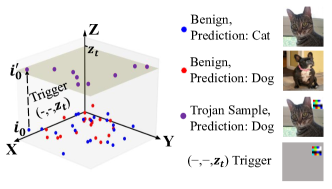
Figure 1: Decision Region of A Trojan Model.

In this paper, we propose a robust training algorithm that can mitigate both injected and natural Trojans. For a given Trojan in the form of $\tilde{\bm{x}}=T(\bm{x},{\bm{m}},{\bm{t}})=({\bm{1}}-{\bm{m}}){\odot}\bm{x}+{\bm{m}}{\odot}\bm{t}$, where $\tilde{\bm{x}}$ and $\bm{x}$ are respectively the poisoning and benign samples, $\tilde{\bm{x}}$ is the poisoning sample generation method using the trigger $(\bm{m},\bm{t})$ with trigger mask matrix $\bm{m}$ and trigger value matrix $\bm{t}$, we theoretically prove that there exists one and only one hyperplane in the input space that corresponds to all poisoning samples. Thus, the trained classifier is mapping this hyperplane to a target label when performing Trojan attacks. Figure 1 intuitively illustrates our idea using a simple example. To simplify the problem, each input has three dimensions $(d_{x},d_{y},d_{z})$. We use red and blue dots to denote inputs belonging to different labels, and the trigger is denoted as $t=(-,-,z_{t})$. Adding the trigger into an input $i_{0}=(x_{0},y_{0},z_{0})$ to get the corresponding Trojaned input $i^{\prime}_{0}=(x_{0},y_{0},z_{t})$ is equivalent to moving this input to the $z=z_{t}$ plane in the input domain. As shown in Figure 1, the input $i_{0}$ moves along the dashed line and ends up in the wheat colored plane, $z=z_{t}$. Notice that $i_{0}$ can be any input, and stamping the trigger will move them to the plane $z=z_{t}$. In other words, the plane $z=z_{t}$ contains all Trojan samples. Likewise, if there exists a plane $z=z_{t}$ that is a decision region, its corresponding input pattern $(-,-,z_{t})$ is a Trojan trigger. Stamping such a trigger to any input is essentially projecting the input to this plane, and because all the inputs in this plane have the same label, it is equivalent to performing a Trojan attack. Extending this to the high dimensional space, the Trojan region will be a hyperplane, and the decision boundaries it shares with other regions will be linear. In summary, we can say that a Trojan in a DNN always pairs with a hyperplane as its Trojan region. Considering that modern DNNs are non-linear and non-convex, this rarely happens for benign models. By further analysis, we found that this is related to the use of activation functions. Modern DNNs tend to use piece-wise linear functions as their activation functions. Even though the function itself is linear, its sub-functions are linear. For example, one of the most popular activation function, ReLU (i.e, $y=\max(0,x)$), consists of two linear functions (i.e., $y=0,x\leq 0$ and $y=x,x>0$). When a model’s weights and biases are trained to specific regions, the neuron values before activation functions will fall into the input domain of only one sub-function (e.g., $x>0$). As a result, the output and input will form a linear relationship. Consequently, the model can generate a hyperplane decision region in the input domain. In other words, we have a hyperplane, denoted as $<x_{0},x_{1},x_{2}>=<a_{0},a_{1},a_{2}>$, as a decision region, and for a given input $i$, if we replace its values in dimensions $x_{0}$, $x_{1}$ and $x_{2}$ to $a_{0}$, $a_{1}$ and $a_{2}$, respectively, we can turn its output label to a desired one. A model training process includes randomness (e.g., random initiation values, optimization), which we cannot avoid. Many possible decision regions will give us the same or similar training/validation accuracy. Some training will learn a linear decision region while others will not. This explains the cause of DNN Trojans and answers the former question, which moves forward our understanding of DNN Trojans one more step.

Based on this analysis, we develop a revised training method, NONE (NON-LinEarity) that identifies linear decision regions, filters out inputs that are potentially poisoned, and resets affected neurons to enforce non-linear decision regions during training. We evaluated our prototype built with Python and PyTorch on MNIST, GTSRB, CIFAR, ImageNet, and the TrojAI dataset. Compared with SOTA methods, NONE is more effective and efficient in mitigating different Trojan attacks (i.e., single-target attack, label-specific attack, label-consistent attack, natural Trojan attack, and the hidden trigger attack). For example, on average, the ASR (attack success rate) of the models trained with NONE is 54.83 times lower than undefended models under standard poisoning Trojan attack and 1.75 times lower under the natural Trojan attack.

Our contributions in this paper can be summered as follows. We analyze the cause of (injected and natural) DNN Trojans and conclude that linearity in DNN decision regions is the main reason. Further, we analyzed the source of linear DNN decision regions and explained why and when it happens using commonly used layers and activation functions. Then, we propose a novel and general revised training framework, NONE that detects and fixes injected and natural Trojans in DNN training. To the best of our knowledge, we are the first to defend natural Trojans. We evaluate NONE on five different datasets and five different Trojans and compare it with other SOTA techniques. Results show that NONE significantly outperforms these prior works in practice.

2 Related Work

Trojans in DNN. Prior work [1, 10, 11, 12, 13, 14, 2, 3, 15, 16, 17, 18] demonstrates that the attackers can inject Trojans into the victim models by poisoning the training dataset. Later, researchers found that a DNN trained on the benign dataset with standard training procedure can also learn such Trojans, which is known as natural Trojans. By using reverse engineering methods designed for poisoned models, researchers were able to find natural triggers in pretrained models. For example, in ABS [8], authors show that a Network in Network (NiN) [19] model trained on a benign CIFAR-10 dataset has natural Trojans. Other works [14, 20] also documented similar findings in other models.

Trojan Defense. One way to defend against Trojan attacks is to filter out poisoning data before training [21, 22]. Poison suppression defenses [23, 24] restrain the malicious effects of poisoning samples in the training phase. Du et al. [23] and Hong et al. [24] apply DP-SGD [25] to depress the malicious gradients brought from poisoned samples. However, existing anti-backdoor learning methods are based on weak observations and they do not find the root cause of Trojans. They can be bypassed by adaptive attacks. In addition, they can not defend natural Trojans. For example, the SOTA anti-backdoor learning method ABL [9] is based on the observation that learning of backdoor behaviors and benign behaviors are distinctive. In detail, the training loss on backdoor examples drops much faster than that on benign examples in the first few epochs. It can be bypassed by slow poisoning attacks. More specifically, when the backdoor attack is label-specific (i.e., the samples with different original labels have different target labels) with low poisoning ratios, the model will learn backdoor behavior slower. We run ABL on the label-specific BadNets attack [1] with ResNet18 model and GTSRB dataset. The results show that the attack success rate is 93.93%, meaning that ABL can not defend against such an attack. This is not surprising because the label-specific attack is more complex, and it is based on the benign behavior of the models (i.e., the model needs to classify the original label of the backdoor examples first, then convert it to corresponding target labels). Another line of work tries to detect if a model has Trojan or not before its deployment. Model diagnosis based defenses [26, 27, 28, 29, 30, 31, 32, 33, 34, 35] determine if a given model has a Trojan or not by inspecting the model behavior. Model reconstruction based defenses try to eliminate injected Trojans in infected models [36, 37, 38, 39, 40], which requires retraining the model with a set of benign data. Another approach is to defend Trojan attacks at runtime. Testing-based defenses [41, 42, 43] judge if the given input contains trigger patterns and reject the ones that are malicious.

3 Methodology

Threat Model. In this paper, we consider training time defense against Trojan attacks, which is also used by existing works [24, 22, 21]. The training dataset can contain poisoning samples (to inject intended Trojans) or benign (but leads to natural Trojans). As defenders, we control the training process but do not assume control over training datasets. Adopted from existing work [26, 41, 42, 27], Trojan sample generation can be formalized as Eq. 1, where $\bm{x}$ and $\tilde{\bm{x}}$ respectively are the benign input and Trojan input. $\bm{m}$, $\bm{t}$ respectively represent, mask of the trigger (i.e., whether a pixel is in the trigger region) and contents of the trigger. $\odot$ is the element-wise multiplication operation on two vectors, i.e., the Hadamard product.

$$\tilde{\bm{x}}=T(\bm{x},\mathchoice{\leavevmode\hbox to8.78pt{\vbox to4.31pt{\text{[drawing]}}}}{\leavevmode\hbox to8.78pt{\vbox to4.31pt{\text{[drawing]}}}}{\leavevmode\hbox to6.15pt{\vbox to3.01pt{\text{[drawing]}}}}{\leavevmode\hbox to4.39pt{\vbox to2.15pt{\text{[drawing]}}}},\mathchoice{\leavevmode\hbox to3.61pt{\vbox to6.15pt{\text{[drawing]}}}}{\leavevmode\hbox to3.61pt{\vbox to6.15pt{\text{[drawing]}}}}{\leavevmode\hbox to2.53pt{\vbox to4.31pt{\text{[drawing]}}}}{\leavevmode\hbox to1.81pt{\vbox to3.08pt{\text{[drawing]}}}})=({\bm{1}}-{\bm{m}})\mathchoice{\leavevmode\hbox to7.78pt{\vbox to6.67pt{\text{[drawing]}}}}{\leavevmode\hbox to7.78pt{\vbox to6.67pt{\text{[drawing]}}}}{\leavevmode\hbox to5.44pt{\vbox to4.67pt{\text{[drawing]}}}}{\leavevmode\hbox to3.89pt{\vbox to3.33pt{\text{[drawing]}}}}\bm{x}+{\bm{m}}\mathchoice{\leavevmode\hbox to7.78pt{\vbox to6.67pt{\text{[drawing]}}}}{\leavevmode\hbox to7.78pt{\vbox to6.67pt{\text{[drawing]}}}}{\leavevmode\hbox to5.44pt{\vbox to4.67pt{\text{[drawing]}}}}{\leavevmode\hbox to3.89pt{\vbox to3.33pt{\text{[drawing]}}}}\bm{t} {\bm{m}} {\bm{t}} \odot \odot {\bm{m}} {\bm{t}} \odot \odot$$ (1)

3.1 Trojan Analysis

To facilitate our discussion, we first define decision region which includes all samples with the same predicted label. Formally, we define it as:

Definition 3.1.

(Decision Region) For a deep neural network $\mathcal{M}:\mathcal{X}\mapsto\mathcal{Y}$ where $\mathcal{X}$ is the input domain $\mathbb{R}^{m}$ and $\mathcal{Y}$ is a set of labels $\{1\ldots k\}$, a decision region is an input space $\mathcal{R}^{l}\subseteq\mathcal{X}$, s.t., $\forall\bm{x}\in\mathcal{R}^{l},\mathcal{M}(\bm{x})=l$.

In most tasks, decision regions with the same label spread over the whole input space because natural inputs belonging to the same label are naturally distributed in this way. Similarly, we define Trojan Decision Region, or in short, we call it the Trojan Region, which is a subregion of the target label decision region:

Definition 3.2.

(Trojan Region) For a Trojaned deep neural network $\mathcal{M}:\mathcal{X}\mapsto\mathcal{Y}$ with target label $l$, its Trojan regions are input spaces where $\mathcal{T}\subseteq\mathcal{R}^{l}$, s.t., all Trojan inputs $\tilde{\bm{x}}\in\mathcal{T}$, and all inputs in $\mathcal{T}$ are Trojan inputs.

Based on the definitions, we have the following theorem:

Theorem 3.3.

Given a model $\mathcal{M}:\mathcal{X}\mapsto\mathcal{Y}$ with the Trojan trigger $(\bm{m},\bm{t})$, if the attack is complete (100% attack success rate) and precise (no other triggers), there exists one and only one hyperplane $\{{\bm{A}}{\bm{x}}-{\bm{b}}=0\}$ Trojan region, where $i\in\{1\ldots m\}$, diagonal matrix ${{\bm{A}}_{i,i}}={\bm{m}}_{i},\bm{b}={\bm{A}}{\bm{t}}$.

The proof for Theorem 3.3 and empirical results are in Appendix (§ 8.1). The theorem shows that when a model learns a Trojan, it essentially learns a hyperplane as a decision region. Based on the definition of decision regions, we know that they are inverse functions of the model. Thus, the inverse function of the Trojan is a hyperplane. To understand how popular model architectures learn such hyperplanes in practice, we perform further analysis.

We start our discussion from typical Convolutional Neural Networks (CNNs). A convolutional layer with activation functions can be represented as $y_{j}=\sigma(\mathbf{W}_{j}^{\mathbf{T}}x_{j}+\mathbf{b}^{\mathbf{T}}_{j})$, where $x_{j}$ and $y_{j}$ are the inputs and outputs of layer $j$, $\mathbf{W}_{j}$ and $\mathbf{b}_{j}$ are trained weights and bias values, and $\sigma$ represents the activation function which is used to introduce non-linearity in this layer. Most commonly used activation functions, e.g., ReLU, are piece-wise linear. For example, ReLU is defined as $\sigma(x)=\max(0,x)$, which consists of two linear pieces separated at $x=0$. As pointed out by Goodfellow et al. [44], even non-piece-wise linear functions are trained to semi-piece-wise linear. This helps resolve the gradient explosion/vanishing problem and makes training DNNs more feasible.

We make a key observation that DNN Trojans will increase linearity of a convolutional layer with activation functions by introducing a large percentage of neurons activating on one piece of the activation function. Specifically, we observe that when the Trojan behavior happens, the neuron values before activation functions fall into one input range of the activation function, which makes it linear. Recall that most well-trained activation functions are piece-wise linear, and if the inputs are in one input range, it regresses to a linear function. For example, layer $j$ using ReLU as its activation function will be a linear layer if $\mathbf{W}_{j}^{\mathbf{T}}x_{j}+\mathbf{b}^{\mathbf{T}}_{j}\geq 0$ for all $x_{j}$. As such, the reverse function of the Trojan can be a hyperplane or overlaps significantly with the hyperplane.

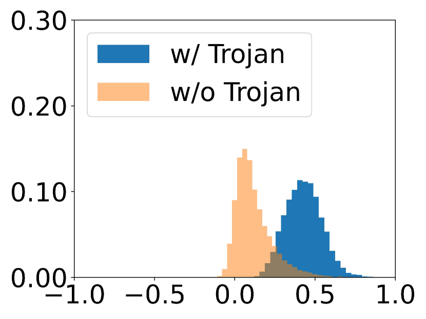
(a) Compromised

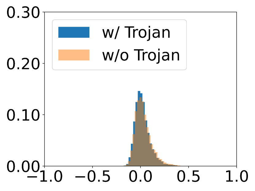
(b) Benign

Figure 2: Comparison of Activation Values.

Figure 2 shows the empirical comparison of a benign model and a Trojan model. In our experiment, we train a benign model $\mathcal{M}$ and a Trojan model $\mathcal{M}^{\prime}$ using ResNet18 on CIFAR-10. While training $\mathcal{M}^{\prime}$, we adopt the TrojanNet [45] training method which guarantees that only certain neurons will contain the Trojan, which we call Trojan neurons. The x-axis in Figure 2 shows the value of $\mathbf{W}^{\mathbf{T}}x+\mathbf{b}^{\mathbf{T}}$, and y-axis shows the percentage of Trojan neurons whose activation value is the corresponding value on x-axis. We use blue color to denote experiments when inputs have the trigger and orange to denote when inputs do not contain the trigger. As we can see, the model that contains the Trojan will activate the $x>0$ region when the input contains the trigger. By contrary, all the other three cases do not have such a phenomenon. We also conduct similar experiments on other different models and different types of layers including non-piece-wise linear layers, and all empirical results confirm our observation here. Details are in Appendix (§ 8.2).

4 Training Algorithm

Algorithm 1 Training

Input:   Training Data: $D$, Maximal epoch: $E$
Output:   Model: $M$

1:function Training($D$)

2:     while $e\leq E$ and (not ${\rm terminate}(M)$) do

3:         $\triangleright$ Train and gather activation values

4:         $M={\rm train}(D,e)$

5:         $A=M.{\rm predict}(D)$

6:         $\triangleright$ Identify compromised neurons

7:         $C=\emptyset$

8:         for neuron $n$ in $M$ do

9:              if  $\mathbb{P}(A_{n}\geq 0)\geq\theta$  then

10:                  $C=C\cup\{n\}$                        

11:         $\triangleright$ Identify biased or poisoning samples

12:         for neuron $n\in C$ do

13:              $B_{n},O_{n}={\rm separate}(A_{n})$

14:              $\mu,\sigma={\rm norm(}B_{n}{\rm)}$

15:              for activation value of input $i:i_{n}\in O_{n}$ do

16:                  if $\left|\frac{i_{n}-\mu}{\sigma}\right|\geq\lambda$ then

17:                       $D=D-{i}$                                          

18:         $\triangleright$ Resetting compromised neurons

19:         for neuron $c\in C$ do

20:              $c=M.{\rm init}(c)$               

To solve the Trojan problem caused by high linearity neurons, we propose Algorithm 1 to enforce non-linearity in individual layers by resetting potentially linear neurons and removing data samples that cause such linearity. This is a revised training process, which is an iterative process that trains the model until the maximal epochs (line 2). It starts by training the model using the standard backward propagation method (line 4). We also gather all activation values of individual neurons $A$ for all training samples in the training dataset $D$. Then, the process contains three steps: identifying compromised neurons (lines 6 to 10), identifying biased or poisoning samples (lines 11 to 17), and lastly, resetting the neurons for retraining (lines 18 to 20).

The first step is to identify comprised neurons, namely the neurons that carry Trojans. Based on our discussion on § 3.1, we do this by checking the activation values of neuron $n$, denoted as $A_{n}$, to see if its function is highly linear using the condition $\mathbb{P}(A_{n}\geq 0)\geq\theta$. If so, we make the neuron $n$ as potentially compromised and add it to the candidate set $C$. The second step is to identify highly biased samples or poisoning samples. The overall design is a statistical testing process: we first find a reference distribution of a particular neuron and then mark all inputs whose activation values do not follow such distributions as potentially biased or poisoning samples. The idea of finding a benign distribution is that inputs whose activation values in a layer are non-linear will be considered as benign and the distribution that describes their activation values is used as the reference distribution. In Algorithm 1, line 13 uses a function to test the linearity of activation values and separate all activation values into a benign set $B$ and others $O$. Then, we normalize the distribution of our reference distribution $B$ to a normal distribution and obtain its mean value $\mu$ and standard deviation value $\sigma$ (line 14). For a single input $i$, we perform a statistical test to see the probability of $i$ being a potentially biased or poisoning sample (lines 15 to 16). We exclude it from the training dataset (line 17). The last step of our training algorithm is to remove the compromised neuron effects from the model by resetting them. We reuse the initialization method in our training setting to set a new value for all identified compromised neurons (line 19 and 20). Then, we continue the training until terminating conditions are met, or the training budget is used up (line 2). This algorithm uses ReLU as an example, and because our theory still holds for other activation functions (see § 8.2), the algorithm can generalize to other models by modifying corresponding parameters (line 9).

To identify compromised neurons and biased/poisoning images, we need to determine the threshold value $\theta$ (line 9) and separate the activation values into non-linear and linear ones. In our implementation, we perform the Fisher’s linear discriminant analysis (its binary version, Otsu’s method [46]) and leverage the Jenks natural breaks optimization algorithm to find the separations of non-linear and linear activation values. Sets $B$ and $O$ are outputs of such algorithms, and we use the standard value that evaluates the quality of such separation to compute the value of our threshold $\theta$, i.e., $0.95$ in our case. Notice such values can affect the accuracy of identifying compromised neurons and inputs. We also choose alternative ways to separate the sets and present the results in the Appendix to evaluate our approach. Similar to model pruning and fine-tuning, when we reset different numbers of neurons (lines 19 and 20), the accuracy on benign and Trojan samples can be different. We present more details of the algorithm and evaluate the sensitivity of NONE to the number of neurons reset during training and identify malicious samples in Appendix (§ 8.8).

5 Experiments

NONE is implemented in Python 3.8 with PyTorch 1.7.0 and CUDA 11.0. If not specified, all experiments are done on a Ubuntu 18.04 machine equipped with six GeForce RTX 6000 GPUs, 64 2.30GHz CPUs, and 376 GB memory. We first introduce the experiment setup (§ 5.1). Then, we evaluate the overall effectiveness of NONE (§ 5.2) and investigate its robustness against different attack settings (§ 5.3). We also evaluate the generalization of NONE on real-world applications (§ 5.4). Finally, we measure the precision and the recall in the poisoned samples identification stage (§ 5.5). Other results and discussions are in Appendix.

5.1 Experiment Setup.

Datasets and Models. We evaluate NONE on five publicly available datasets: MNIST [47], GTSRB [48], CIFAR-10 [49], ImageNet-10 [50] and TrojAI [51]. The overview of our datasets and more details can be found in § 8.5. Figure 3 illustrates different trigger patterns used in the experiments (i.e., a single pixel located in the right bottom corner of 3(a), a fixed red patch in 3(b), a black-and-white pattern whose location is random in 3(c) and a colorful watermark in  3(d)). The default trigger pattern for MNIST, CIFAR-10, GTSRB, and ImageNet-10 are Single Pixel (3(a)), Static Patch (3(c)), Dynamic Patch (3(b)) and Watermark (3(d)), respectively. Besides the default triggers for each dataset, we also measure the impacts of using other triggers. The results are included in § 5.3. We evaluate NONE and other defense methods on AlexNet [50], NiN (Network in Network) [19], VGG11, VGG16 [52] and ResNet18 [53]. These models are representative and are commonly used in existing Trojan related studies [8, 26].

(a) Single Pixel

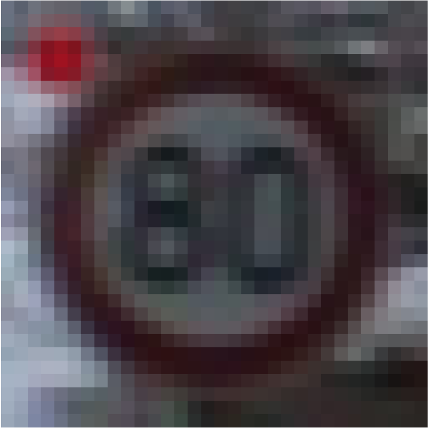
(b) Static

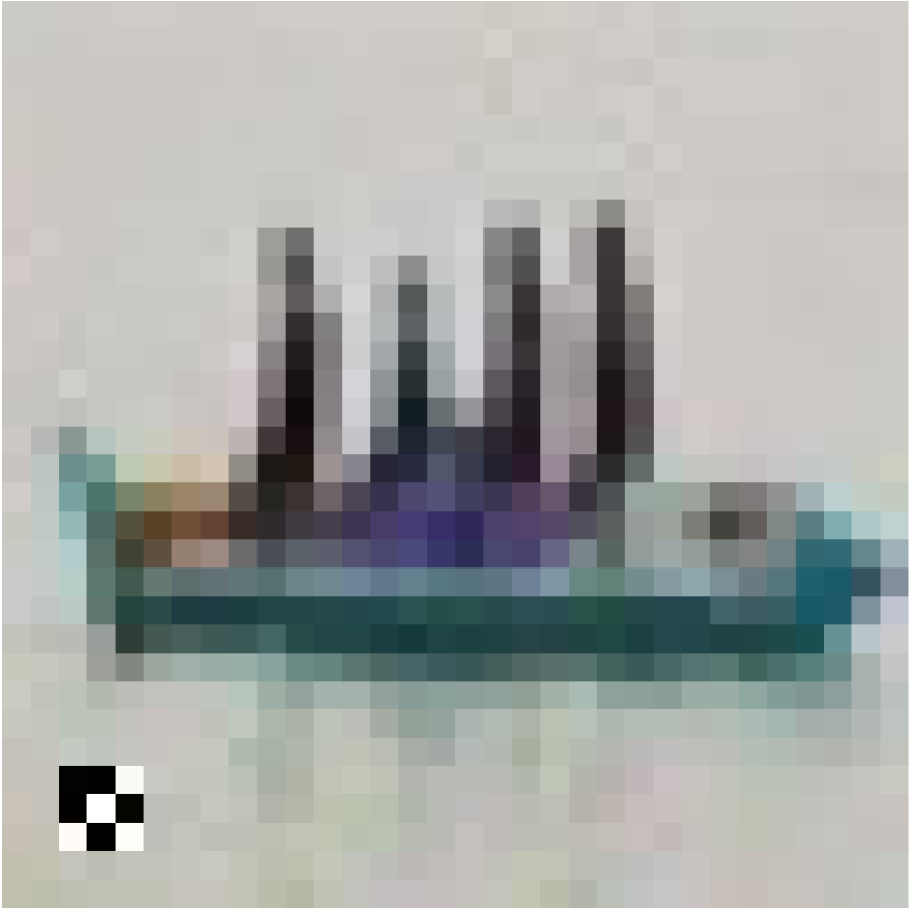
(c) Dynamic

(d) Watermark

Figure 3: Examples of Using Different Trigger Patterns.

Evaluation Metrics. We use benign accuracy (BA) and attack success rate (ASR) [54] as evaluation metrics, which is a common practice [55, 41, 26]. BA is defined as the number of correctly classified benign samples over the number of all benign samples. It implies model’s capability on its original task. ASR evaluates the success rate of backdoor attacks. It is calculated as the number of backdoor samples that can successfully attack the model over the number of all generated backdoor samples.

Attack Settings. As we introduced in § 2, Trojans are classified into two categories: Injected Trojans and Natural Trojans. We implement both of them to evaluate NONE and other defense methods. For Injected Trojans, we implement both single target and label specific BadNets [1], label-consistent Trojan attack [11] and hidden trigger Trojan attack [56]. Following the original paper, we use images from a pair of classes (class theater curtain and class plunger) in ImageNet for hidden trigger Trojan attack. For natural Trojans, we follow the previous work [8] to reproduce the attack. Due to the fact that we do not know if the data is poisoned or not in advance, NONE keeps detecting Trojan attacks and training the model even if there is no attack activity. We evaluate the additional costs of NONE on benign models in such non-attack settings. More details for our attack settings are included in § 8.6. Besides above attacks, We also evaluate the generalization of NONE on more attacks in § 8.7.

Comparison. We compare NONE with 4 state-of-the-art defense methods: DP-SGD [24], Neural Attention Distillation (NAD) [38], Activation Clustering (AC) [22] and Anti-backdoor Learning (ABL) [9]. We use their official code and default hyperparameters specified in the original papers.

5.2 Effectiveness of NONE

Table 1: Comparisons on Injected Trojans.

Attack Type	Dataset	Network		Undefended			DP-SGD			NAD			AC			ABL			NONE
				BA	ASR		BA	ASR		BA	ASR		BA	ASR		BA	ASR		BA	ASR
BadNets (single target)	MNIST	NiN		99.65%	99.96%		92.94%	0.48%		99.26%	0.06%		98.47%	0.51%		98.25%	99.70%		99.58%	0.06%
		VGG11		99.35%	100.00%		97.20%	1.61%		98.85%	2.12%		97.44%	10.93%		98.48%	0.64%		99.11%	0.14%
		ResNet18		99.61%	99.98%		97.31%	0.13%		98.83%	0.12%		98.04%	0.25%		99.34%	0.04%		99.57%	0.37%
	CIFAR-10	NiN		90.52%	100.00%		36.41%	93.01%		80.99%	52.97%		83.77%	100.00%		90.13%	100.00%		90.11%	2.32%
		VGG16		90.46%	100.00%		55.61%	99.32%		88.70%	98.71%		88.14%	99.84%		89.96%	100.00%		89.70%	4.91%
		ResNet18		94.10%	100.00%		52.29%	99.99%		88.74%	1.28%		89.57%	57.43%		92.40%	1.66%		93.62%	1.07%
	GTSRB	NiN		95.95%	99.72%		31.54%	74.78%		96.53%	26.15%		95.36%	99.52%		96.14%	99.54%		95.51%	0.87%
		VGG16		95.43%	99.93%		54.60%	86.83%		95.94%	86.10%		91.28%	5.28%		94.06%	95.79%		94.66%	0.96%
		ResNet18		96.67%	99.84%		55.73%	90.88%		95.95%	13.18%		94.64%	98.57%		96.24%	0.93%		96.39%	0.76%
	ImageNet-10	NiN		82.17%	99.64%		21.22%	65.21%		76.99%	92.61%		74.32%	92.41%		81.35%	99.92%		80.31%	0.14%
		VGG16		88.97%	100.00%		18.06%	44.62%		84.03%	10.93%		81.58%	100.00%		79.16%	100.00%		87.11%	0.14%
		ResNet18		89.83%	99.07%		40.31%	29.58%		86.29%	25.89%		82.39%	98.44%		83.72%	6.83%		86.34%	0.08%
BadNets (label specific)	MNIST	NiN		99.64%	98.86%		93.02%	1.10%		99.24%	0.09%		99.60%	0.03%		98.40%	89.32%		99.42%	0.03%
		VGG11		99.05%	98.99%		97.17%	0.41%		99.06%	32.06%		97.59%	0.10%		99.21%	98.51%		98.63%	0.11%
		ResNet18		99.57%	99.49%		96.81%	0.38%		99.19%	0.19%		99.35%	0.03%		99.01%	98.81%		99.09%	0.20%
	CIFAR-10	NiN		90.50%	78.56%		38.42%	6.43%		82.70%	13.65%		84.74%	56.57%		89.66%	77.69%		89.51%	1.27%
		VGG16		90.73%	96.86%		55.12%	5.23%		88.65%	39.99%		88.18%	82.87%		90.13%	86.91%		89.64%	1.22%
		ResNet18		94.37%	92.00%		52.19%	12.17%		88.21%	1.50%		92.68%	5.29%		83.83%	83.48%		93.05%	1.04%
	GTSRB	NiN		96.06%	93.74%		24.70%	7.39%		96.46%	9.90%		94.02%	6.17%		96.14%	99.54%		95.99%	0.96%
		VGG16		95.71%	94.57%		53.90%	6.71%		96.33%	81.43%		94.96%	69.22%		94.32%	80.21%		95.49%	1.65%
		ResNet18		96.93%	97.40%		60.59%	6.61%		95.49%	11.13%		95.74%	1.16%		90.24%	93.93%		96.63%	0.91%
	ImageNet-10	NiN		82.65%	66.37%		23.44%	10.06%		76.31%	23.31%		78.85%	14.39%		80.20%	56.82%		79.39%	6.98%
		VGG16		89.04%	76.20%		17.94%	10.80%		80.21%	22.17%		81.22%	59.62%		78.34%	53.68%		84.51%	8.31%
		ResNet18		88.87%	59.75%		44.59%	7.95%		85.76%	15.82%		79.44%	23.41%		81.30%	50.52%		84.74%	6.55%
Label consistent	CIFAR-10	NiN		91.32%	98.98%		38.83%	5.21%		82.35%	65.63%		83.92%	95.96%		89.95%	95.28%		90.11%	2.19%
		VGG16		90.97%	98.41%		53.76%	9.24%		88.88%	92.71%		88.46%	7.57%		90.38%	94.94%		90.07%	4.26%
		ResNet18		94.73%	83.42%		54.00%	11.00%		90.74%	60.74%		88.00%	65.86%		87.34%	2.17%		94.01%	2.14%
Hidden Trigger	ImageNet-pair	AlexNet		93.00%	82.00%		80.00%	62.00%		91.00%	74.00%		90.00%	22.00%		90.00%	54.00%		91.00%	4.00%

Table 2: Comparisons on Natural Trojan.

Dataset	Network		Undefended			DP-SGD-1			DP-SGD-2			NONE
			BA	ASR		BA	ASR		BA	ASR		BA	ASR
CIFAR-10	NiN		91.02%	87.62%		60.22%	98.85%		39.19%	87.22%		86.94%	34.21%
	VGG16		90.78%	71.88%		78.25%	61.11%		53.40%	63.58%		81.83%	37.49%
TrojAI	VGG11		99.88%	72.09%		84.51%	88.75%		6.06%	88.55%		99.04%	56.68%
	Resnet18		99.91%	54.33%		78.88%	61.77%		52.81%	58.94%		98.13%	34.98%

Experiments. We measure the effectiveness of NONE by comparing the BA and ASR of models protected by NONE with those of undefended models and models protected by existing defense methods. The comparison results on injected Trojans, natural Trojans and non-attack settings are shown in Table 1, Table 2 and Table 4, respectively. In each table, we show the detailed settings including attack settings, dataset names and network architectures., etc. For the evaluation results on natural Trojans ( Table 2), the ASR and BA are the average results under different trigger size settings: 2%, 4%, 6%, 8%, 10% and 12% of the whole image. Notice that, to the best of our knowledge, there is no defense method designed for natural Trojans. We observe that DP-SGD can potentially mitigate natural Trojans because it reduces the high gradients brought from natural Trojans. Therefore, we adapt DP-SGD as the baseline method for natural Trojans. We configure DP-SGD with two settings of parameters following the prior work [24]. For DP-SGD-1, we set the clip as 4.0 and the noise as 0.1. The clip and noise of DP-SGD-2 are 1.0 and 0.5. For the non-attack settings, we deploy NONE on several benign models and show the decrease of BA in Table 4.

Results on Injected Trojans. From the results on Injected Trojan attacks (Table 1), we observe that applying NONE can better protect models from being attacked by injected Trojans than other defense methods. With NONE, the average ASR of models decreases from 93.34% to 1.91%, which is much better than other defense methods (DP-SGD, NAD, AC and ABL can only reduce the average ASR to 30.32%, 34.08%, 45.45% and 68.60% respectively). The reason is that, unlike existing methods based only on specific empirical observations, NONE targets the root cause of the Trojans (i.e., the linearity) and reveals the attacks more accurately. Therefore, NONE can better defend against attacks than other methods.

We also find that NONE almost does not have negative impacts on the original task of models. From Table 1, the BA of NONE is the highest among all methods and is similar to that of undefended models, meaning that NONE has a low defense cost. The reason is that NONE only modifies the compromised neurons that are highly relevant to Trojan but less related to the original task of models. Therefore, most of the benign knowledge is preserved when applying NONE and the model can still perform well on its original tasks. Meanwhile, NONE finetunes the model on the purified data after the reset process, further strengthening the capabilities of models and reducing defense costs.

It is worth clarifying that ABL has a poor performance on label-specific attacks and other attacks that use NiN and VGG models. The possible reason is that the design of ABL requires the model to learn quicker and better on Trojan samples than benign samples [9] (i.e., the learning of Trojan samples should have a lower training loss value in the early training stage). When the attacker uses more complex attacks (e.g., label specific BadNets) or models with limited learning capabilities (e.g., NiN and VGG), the model cannot learn Trojan samples quickly, leading to poor performance.

Results on Natural Trojans. From the results in  Table 2, we find that NONE protects the model most effectively and has the lowest defense costs among all defense methods. Overall, applying NONE achieves 1.75 times lower ASR than undefended models. DP-SGD methods can only slightly decreases ASR or even increase ASR. The results show that using NONE is the most effective way for natural Trojan defense. The loss of BA using NONE is also smaller than the loss caused by applying the DP-SGD methods (3.90% with NONE and 38.76% with DP-SGD methods on average), further showing the efficiency of NONE. The results confirm our analysis: reducing the linearity of models reduces the ASR of natural Trojans without posing much additional cost.

Results on Non-attack Setting. We also explore whether NONE affects the performance of benign models on their original tasks. From Table 4, we find that NONE has a low effect on benign models. Applying NONE only decreases 2.33% BA on average. Because only a few neurons are detected as compromised neurons and are reset by NONE when there is no Trojan activity, NONE does not affect the learned benign knowledge. Moreover, the subsequent training process further reduces the costs. Therefore, we conclude that NONE does not impose high additional costs on benign models.

Table 3: Benign Accuracy in Non-attack Settings.

Dataset	Network	Without NONE	With NONE
CIFAR-10	NiN	91.02%	89.40%
	VGG16	90.78%	89.62%
	ResNet18	94.83%	93.92%
GTSRB	NiN	95.68%	95.36%
	VGG16	94.67%	94.08%
	ResNet18	96.89%	96.87%
ImageNet-10	NiN	83.34%	79.18%
	VGG16	88.84%	83.41%
	ResNet18	89.81%	85.25%

Table 4: Results on Different Trigger Patterns.

Trigger Pattern	Network	Undefended			NONE
		BA	ASR		BA	ASR
Dynamic Patch	NiN	90.52%	100.00%		90.11%	2.32%
	VGG16	90.46%	100.00%		89.70%	4.91%
	ResNet18	94.10%	100.00%		93.62%	1.07%
Static Patch	NiN	90.92%	100.00%		89.93%	2.61%
	VGG16	90.12%	100.00%		89.48%	4.03%
	ResNet18	94.24%	99.99%		93.93%	1.37%
Watermark	NiN	90.88%	99.99%		87.74%	3.27%
	VGG16	90.64%	99.99%		89.14%	5.36%
	ResNet18	94.28%	100.00%		92.27%	5.99%

Table 5: Results on Different Trigger Sizes.

Trigger Size	Undefended			NONE
	BA	ASR		BA	ASR
3*3	94.10%	100.00%		93.62%	1.07%
5*5	94.27%	100.00%		93.51%	1.34%
7*7	94.10%	99.98%		93.70%	1.53%
9*9	94.34%	100.00%		93.19%	5.18%
15*15	94.44%	100.00%		92.18%	32.27%
20*20	94.58%	100.00%		92.55%	99.82%

Table 6: Results on Different Poisoning Rates.

Poisoning rate	Undefended			NONE
	BA	ASR		BA	ASR
0.50%	94.46%	100.00%		93.50%	2.52%
5.00%	94.10%	100.00%		93.62%	1.07%
10.00%	93.82%	100.00%		93.13%	1.04%
20.00%	92.70%	100.00%		92.14%	1.39%

5.3 Robustness of NONE

We evaluate the robustness of NONE against various attack settings (e.g., different trigger sizes, trigger patterns and poisoning rates). If not specified, the model used in the evaluation is ResNet18. The dataset is CIFAR-10 and the evaluated attack is the single target BadNets attack.

Trigger Sizes. To study the effects of trigger size, we use triggers of different sizes (from 3*3 to 20*20) to attack models and collect the ASR and BA of applying NONE on these compromised models. The results are shown in Table 6. Overall, the BA of undefended models and models protected by NONE is insensitive to the change of trigger size. The difference between the highest and lowest BA on the unprotected and protected models is 0.48% and 1.52%, respectively, which is very small. We believe that the BA does not change significantly because triggers usually do not affect the learning of benign features used for original tasks, as discussed in previous work [1].

On the other hand, the trigger size affects the ASR of protected models. When the trigger size becomes larger, the ASR of the protected model increases dramatically from 1.07% to 99.82% and NONE fails. The results are understandable because a large trigger size modifies more pixels in the original image, making the triggers obvious and easy to learn. When the trigger is large, it almost covers the whole image and becomes the majority of the image. In such a scenario, models easily capture trigger features and are compromised. A detailed example is shown in Figure 12. Currently, the sensitivity to trigger sizes is a common limitation for Trojan defense methods [26, 8]. Considering that a large trigger size is almost impractical because it makes the trigger too obvious to be detected directly by administrators, we consider NONE robust to most trigger sizes.

Trigger Patterns. To measure the robustness of NONE against different attack trigger patterns, we use NONE to protect models from being attacked by Dynamic Patch trigger, Static Patch trigger and Watermark trigger. The results are shown in Table 4. We observe that NONE always achieves low ASR and high BA under different trigger settings. The results demonstrate that NONE is effective against different trigger pattern settings. Moreover, we notice that the ASR of using the watermark trigger is particularly larger compared with using other triggers. The reason is that the watermark triggers are large and more complex, as shown in Figure 3.

Poisoning Rates. To measure the impacts of different poisoning rates, we collect the ASR and BA of models being compromised at different poisoning rates from 0.50% to 20.00%. The results are summarized in  Table 6. Based on the results, we find that increasing the poisoning rate slightly decreases both the BA and ASR. Specifically, the BA of the model decreases by 1.36% and the ASR of the model decreases by 1.13%. This is because increasing the poisoning rate reduces the number of benign samples used for training, and the BA of the model naturally decreases. Meanwhile, a large poisoning rate makes Trojans easy to be detected, which leads to a lower ASR. Since the changes in ASR and BA are quite small, NONE is considered robust to most poisoning rates.

Table 7: Results on Federated Learning.

Dataset	Undefended			NONE
	BA	ASR		BA	ASR
MNIST	99.22%	99.15%		98.60%	0.13%
CIFAR-10	80.31%	43.23%		78.67%	4.44%

5.4 Generalization on Complex Applications

Attackers may conduct attacks in a more complex scenario. To measure the generalization of NONE on complex applications, we evaluate NONE on two federated learning applications trained on different datasets (i.e., MNIST and CIFAR-10) and a transfer learning application. Each federated learning application has 10 participants, of which 4 of them are malicious participants who conduct the distributed Trojan attacks [7] jointly to inject Trojan triggers into the global model. We assume that attackers train their local models on the poisoned training data and contribute to the global model without scaling the original weight of the poisoned local models. We then apply NONE on the global model to defend against the Trojan attack from malicious local models. Specifically, NONE requires the participants to use their data to test the global model and upload the activation values of the global model to identify compromised neurons. To measure the defense performance, we measure the BA and ASR of the global models (i.e., the original model and model deployed with NONE). The results are shown in Table 7. As shown in the table, on average, NONE achieve 31.16 times lower ASR than undefended models with a slight decrease (i.e., 1.13%) in the BA. The results show that NONE can defend against the Trojan attacks effectively in real-world federated learning applications at a low cost. Besides federated learning, we have also discussed the performance of NONE in transfer learning settings. Hidden Trigger Trojan Attack [56] in § 5.2 of the main paper is conducted in transfer learning scenarios and the results are shown in Table 1 of the main paper. As the results show, NONE achieves low ASR (i.e., 4.00%) and high BA (i.e., only 2.00% lower than undefended models), proving the generalization of NONE on transfer learning settings.

5.5 Precision and Recall of the Poisoned Sample Identification

In line 12-17 of Algorithm 1, we identify the poisoned samples in the training data. To evaluate the effectiveness of the identification process, we measure the precision and the recall of detecting poisoned samples on the CIFAR-10 dataset and three different models (i.e., NiN, VGG16, and ResNet18). Results in Table 8 demonstrate the precision and the recall of NONE are always above 98% on different settings. For example, on ResNet18 and Label-consistent attack, both the precision and the recall of NONE are 100.00%. Thus, NONE can detect poisoned samples accurately.

Table 8: Precision and Recall of Poisoned Samples Identification.

Attack		NiN			VGG16			ResNet18
		Precision	Recall		Precision	Recall		Precision	Recall
BadNets		99.60%	99.64%		99.96%	100.00%		99.84%	99.92%
Label-consistent		98.80%	99.20%		100.00%	100.00%		100.00%	100.00%

6 Discussion

In this paper, we focus the discussion on image classification tasks, which is the focus of many existing works [1, 56, 11, 8, 26, 57]. Expanding our work, including the theory and system to other problem domains, such as natural language processing and reinforcement learning, other computer vision tasks, e.g., object detection, will be our future work.

Research on adversarial machine learning potentially has ethical concerns. In this research, we propose a theory to explain existing phenomena and attacks, and propose a new training method that removes Trojans in a DNN model. We believe this is beneficial to society.

In our current threat model, the adversary can only inject poisoning data into the training dataset, and there is no existing adaptive attacks. However, adaptive adversaries can still conduct attacks under other threat models, and we discuss such case in § 8.10.

7 Conclusion

In this paper, we present an analysis on DNN Trojans and find relationships between decision regions and Trojans with a formal proof. Moreover, we provide empirical evidence to support our theory. Furthermore, we analyzed the reason why models will have such phenomena is because of linearity of trained layers. Based on this, we propose a novel training method to remove Trojans during training, NONE, which can effectively and efficiently prevent intended and unintended Trojans.

Checklist

1. For all authors…

   1. Do the main claims made in the abstract and introduction accurately reflect the paper’s contributions and scope? [Yes]

   2. Did you describe the limitations of your work? [Yes] See § 6.

   3. Did you discuss any potential negative societal impacts of your work? [Yes] See § 6.

   4. Have you read the ethics review guidelines and ensured that your paper conforms to them? [Yes] See § 6.

2. If you are including theoretical results…

   1. Did you state the full set of assumptions of all theoretical results? [Yes] See § 3.1.

   2. Did you include complete proofs of all theoretical results? [Yes] See Appendix.

3. If you ran experiments…

   1. Did you include the code, data, and instructions needed to reproduce the main experimental results (either in the supplemental material or as a URL)? [Yes] See Abstract, § 5, and Appendix.

   2. Did you specify all the training details (e.g., data splits, hyperparameters, how they were chosen)? [Yes] See § 5 and Appendix.

   3. Did you report error bars (e.g., with respect to the random seed after running experiments multiple times)? [No]

   4. Did you include the total amount of compute and the type of resources used (e.g., type of GPUs, internal cluster, or cloud provider)? [Yes] See § 5.

4. If you are using existing assets (e.g., code, data, models) or curating/releasing new assets…

   1. If your work uses existing assets, did you cite the creators? [Yes] See § 5.

   2. Did you mention the license of the assets? [Yes] See Appendix.

   3. Did you include any new assets either in the supplemental material or as a URL? [Yes] URL for our code is included in Abstract.

   4. Did you discuss whether and how consent was obtained from people whose data you’re using/curating? [Yes] See Appendix.

   5. Did you discuss whether the data you are using/curating contains personally identifiable information or offensive content? [Yes] See Appendix.

5. If you used crowdsourcing or conducted research with human subjects…

   1. Did you include the full text of instructions given to participants and screenshots, if applicable? [N/A]

   2. Did you describe any potential participant risks, with links to Institutional Review Board (IRB) approvals, if applicable? [N/A]

   3. Did you include the estimated hourly wage paid to participants and the total amount spent on participant compensation? [N/A]

8 Appendix

Roadmap: In this appendix, we first list the symbols we used in this paper. We show the proof and the empirical results for Theorem 3.3 (§ 8.1), more empirical evidence for model’s linearity (§ 8.2), explanation for DP-SGD (§ 8.3), and more details about the sample separation (§ 8.4). Then, we provide implementation details including details of datasets (§ 8.5) and used attacks (§ 8.6). We then discuss the the resistance of NONE against more attacks (§ 8.7), and the efficiency of NONE (§ 8.9). We measure the sensitivity of NONE against different configurable parameters (§ 8.8). We then evaluate NONE on an adaptive attack (§ 8.10). In § 8.11, we compare NONE to another defense DBD [58]. We also compare NONE to more defenses on natural Trojan in § 8.12. Finally, we evaluate the generalization to larger models (§ 8.13) and larger datasets (§ 8.14).

Symbol Table.

Table 9: Summary of Symbols

Scope	Symbol	Meaning
Theory	$\bm{x}$	Benign Sample
	$\tilde{\bm{x}}$	Trojan Sample
	$T$	Trojan Sample Generation Function
	$\bm{m}$	Mask of Trojan Trigger
	$\bm{t}$	Pattern of Trojan Trigger
	$\odot$	Hadamard product
	$\mathcal{M}$	Model
	$\mathcal{X}$	Input Domain
	$\mathcal{Y}$	Set of Labels
	$\mathcal{R}^{l}$	Decision Region of Label $l$
	$\mathcal{T}$	Trojan Region
	$m$	The Number of Elements in $\bm{m}$
	$\{{\bm{A}}{\bm{x}}-{\bm{b}}=0\}$	Trojan Hyperplane
	$x_{j}$	Inputs of Layer $j$
	$y_{j}$	Outputs of Layer $j$
	$\mathbf{W}_{j}$	Trained Weights of Layer $j$
	$\mathbf{b}_{j}$	Trained Bias of Layer $j$
Algorithm	$D$	Training Data
	$E$	Maximal Epoch
	$e$	Current Epoch
	$M$	Model
	$n$	Neuron
	$A$	Activation Values
	$A_{n}$	Activation values on Neuron $n$
	$C$	Compromised Neurons
	$B_{n}$	The Cluster of Smaller Values in $A_{n}$
	$O_{n}$	The Cluster of Larger Values in $A_{n}$
	$\mu$	Mean Value of $B_{n}$
	$\sigma$	Standard Deviation Value of $B_{n}$
	$i$	Input Sample
	$i_{n}$	The Activation Value of Input Sample $i$ on Neuron $n$

8.1 Proof and Empirical Evidence for Theorem 3.3

We start our analysis from ideal Trojan attacks, which we define as complete and precise Trojans:

Definition 8.1.

Complete Trojan: For a Trojaned model $\mathcal{M}:\mathcal{X}\mapsto\mathcal{Y}$ with trigger $(\bm{m},\bm{t})$ and target label $l$, we say a Trojan is complete if $\forall\bm{x}\in T(\mathcal{X},{\bm{m}},{\bm{t}}),\mathcal{M}(\bm{x})=l$.

Definition 8.2.

Precise Trojan: For a Trojaned model $\mathcal{M}:\mathcal{X}\mapsto\mathcal{Y}$ with trigger $(\bm{m},\bm{t})$ and target label $l$, we say a Trojan is precise if the follow condition is met: $\forall(\bm{m}^{\prime},\bm{t}^{\prime})\neq(\bm{m},\bm{t}),\bm{x}^{\prime}=T(\bm{x},{\bm{m}}^{\prime},{\bm{t}}^{\prime}),\mathcal{M}(\bm{x})\neq l\Rightarrow\mathcal{M}(\bm{x}^{\prime})\neq l$.

Intuitively, a complete Trojan means the attack success rate of this attack is 100%, and a precise Trojan means that the trigger is unique: if we change the trigger ($\bm{t}$ or $\bm{m}$), it will not trigger the predefined misclassification.

Proof.

In Theorem 3.3, we have $\textbf{S${}_{0}$}\iff\textbf{S${}_{1}$}$ where:

• S₀: Trojan in $\mathcal{M}$ with trigger being $(\bm{m},\bm{t})$ and target label being $l$ is a complete and precise Trojan.

• S₁: The hyperplane $\{{\bm{A}}{\bm{x}}-{\bm{b}}=0\}$ is the Trojan region of $\mathcal{M}$ and the only one, where $i\in\{1\ldots m\}$, diagonal matrix ${{\bm{A}}_{i,i}}={\bm{m}}_{i},\bm{b}={\bm{A}}{\bm{t}}$.

In this proof, we first prove $\bm{x}\in T(\mathcal{X},{\bm{m}},{\bm{t}})\iff\bm{x}\in\{{\bm{A}}{\bm{x}}-{\bm{b}}=0\}$, and then prove $\textbf{S${}_{0}$}\Rightarrow\textbf{S${}_{1}$}$ and $\textbf{S${}_{1}$}\Rightarrow\textbf{S${}_{0}$}$.

Step 1: $\bm{x}\in T(\mathcal{X},{\bm{m}},{\bm{t}})\Rightarrow\bm{x}\in\{{\bm{A}}{\bm{x}}-{\bm{b}}=0\}$. Let $\tilde{\bm{x}}$ be a Trojan input generated from $\bm{x}$ by applying Eq. 1 (in § 3 of the main paper), $\small\tilde{\bm{x}}=T(\bm{x},{\bm{m}},{\bm{t}})=({\bm{1}}-{\bm{m}})\odot\bm{x}+{\bm{m}}\odot\bm{t}$, we get:

$${\bm{A}}\tilde{\bm{x}}-{\bm{b}}={\bm{A}}(({\bm{1}}-{\bm{m}})\odot\bm{x}+{\bm{m}}\odot\bm{t})-{\bm{b}}$$ (2)

Then, based on the definition of matrix $\bm{A}$, $\bm{b}$, the Hadamard product, and the distributive property of matrix multiplication, we can get the following equation, where ${\bm{E}}$ is the identity matrix:

$${\bm{A}}(({\bm{1}}-{\bm{m}})\odot\bm{x}+{\bm{m}}\odot\bm{t})-{\bm{b}} ={\bm{A}}(({\bm{E}}-{\bm{A}})\bm{x}+{\bm{A}}\bm{t})-{\bm{A}}{\bm{t}}$$ (3)

$$={\bm{A}}({\bm{E}}-{\bm{A}})\bm{x}+{\bm{A}}{\bm{A}}\bm{t}-{\bm{A}}{\bm{t}}$$

Since $\bm{A}$ is a diagonal matrix, and all elements of $\bm{A}$ is 0 or 1 based on the definition of $\bm{A}$ and trigger mask $\bm{m}$, we can get $\bm{A}\bm{A}=\bm{A}$ and $\bm{A}(\bm{E}-\bm{A})=0$. Then, according to Eq. 2 and Eq. 3, we get: $\forall\bm{x}\in T(\mathcal{X},{\bm{m}},{\bm{t}}),\;\;{\bm{A}}{\bm{x}}-{\bm{b}}=0$.

Step 2: $\bm{x}\in\{{\bm{A}}{\bm{x}}-{\bm{b}}=0\}\Rightarrow\bm{x}\in T(\mathcal{X},{\bm{m}},{\bm{t}})$. This step is to prove that any sample in the hyperplane $\{{\bm{A}}{\bm{x}}-{\bm{b}}=0\}$ can be obtained from pasting Trojan trigger on other samples. Let $\tilde{\bm{x}}$ denote any sample in the hyperplane, and ${\bm{x}}$ is the sample that is not in the hyperplane, i.e., an external sample. Any external sample $\bm{x}$ that satisfies $({\bm{E}}-{\bm{A}})\bm{x}=({\bm{E}}-{\bm{A}})\tilde{\bm{x}}$ can be transformed to $\tilde{\bm{x}}$ via the projection specified by ${\bm{m}}$ and ${\bm{t}}$. Therefore, we conclude that any sample in the hyperplane can be obtained by pasting the Trojan trigger on other samples.

Steps 1 and 2 prove that $\bm{x}\in T(\mathcal{X},{\bm{m}},{\bm{t}})$ is equivalent to $\bm{x}$ in the hyperplane ${\bm{A}}{\bm{x}}-{\bm{b}}=0$, namely:

$$\bm{x}\in T(\mathcal{X},{\bm{m}},{\bm{t}})\iff\bm{x}\in\{{\bm{A}}{\bm{x}}-{\bm{b}}=0\}$$ (4)

Step 3: $\textbf{S${}_{0}$}\Rightarrow\textbf{S${}_{1}$}$. Based on S₀, Trojan in $\mathcal{M}$ is a complete Trojan. Based on Eq. 4 and the definition of complete Trojan (i.e., 8.2), we get: $\forall\bm{x}\in\{{\bm{A}}\bm{x}-{\bm{b}}=0\},\mathcal{M}(\bm{x})=l$, which means $\{\bm{A}\bm{x}-{\bm{b}}=0\}$ is a Trojan decision region. We then prove $\{\bm{A}\bm{x}-{\bm{b}}=0\}$ is the only Trojan region using proof by contradiction. For any other hyperplane $\{{\bm{A}}^{\prime}\bm{x}-{\bm{b}}^{\prime}=0\}$ where $({\bm{A}}^{\prime},{\bm{b}}^{\prime})\neq({\bm{A}},{\bm{b}})$, based on Eq. 4, we can get: $(\bm{m}^{\prime},\bm{t}^{\prime})\neq(\bm{m},\bm{t}),\bm{x}^{\prime}=T(\bm{x},{\bm{m}}^{\prime},{\bm{t}}^{\prime})\iff{\bm{A}}^{\prime}\bm{x}^{\prime}-{\bm{b}}^{\prime}=0$. According to S₀, the Trojan is a precise Trojan: $\forall(\bm{m}^{\prime},\bm{t}^{\prime})\neq(\bm{m},\bm{t}),{\bm{x}}^{\prime}=T({\bm{x}},{\bm{m}}^{\prime},{\bm{t}}^{\prime}),\mathcal{M}({\bm{x}})\neq l\Rightarrow\mathcal{M}({\bm{x}}^{\prime})\neq l$. Thus, we get that ${\bm{A}}^{\prime}\bm{x}-{\bm{b}}^{\prime}=0$ is not a Trojan region. That is, the Trojan region has only one hyperplane, $\{\bm{A}\bm{x}-{\bm{b}}=0\}$.

Step 4: $\textbf{S${}_{1}$}\Rightarrow\textbf{S${}_{0}$}$. According to S₁, we have:

$$\forall\bm{x}\in\{{\bm{A}}\bm{x}-{\bm{b}}=0\},\mathcal{M}({\bm{x}})=l$$ (5)

$$\small\forall{({\bm{A}}^{\prime},{\bm{b}}^{\prime})\neq(\bm{A},{\bm{b}}),{\bm{A}}^{\prime}\bm{x}^{\prime}-{\bm{b}}^{\prime}=0},\mathcal{M}({\bm{x}})\neq l\Rightarrow\mathcal{M}({\bm{x}}^{\prime})\neq l$$ (6)

From Eq. 4 and Eq. 5, we get $\forall{\bm{x}\in T(\mathcal{X},{\bm{m}},{\bm{t}})},\mathcal{M}({\bm{x}})=l$, which means the Trojan is complete. Based on Eq. 4 and Eq. 6, we can get $\forall(\bm{m}^{\prime},\bm{t}^{\prime})\neq(\bm{m},\bm{t}),{\bm{x}}^{\prime}=T({\bm{x}},{\bm{m}}^{\prime},{\bm{t}}^{\prime}),\mathcal{M}({\bm{x}})\neq l\Rightarrow\mathcal{M}({\bm{x}}^{\prime})\neq l$, where $\bm{m}^{\prime}=\bm{A}_{i,i}^{\prime},\bm{b}^{\prime}=\bm{A}^{\prime}\bm{t}^{\prime},$ indicating that the Trojan is precise.

From Step 3 and 4, we can conclude that $\textbf{S${}_{0}$}\iff\textbf{S${}_{1}$}$, and complete the proof of Theorem 3.3. ∎

Intuitively, the Trojan is precise means the attack success rate is 100% which guarantees that all samples with the trigger will be classified as the target label. The Trojan is complete means that no other input patterns can trigger this trigger, and thus all inputs that activate this Trojan have this trigger. In the real world, these are hard to achieve. In practice, a Trojan of model $\mathcal{M}$ whose trigger is $(\bm{m},\bm{t})$ and target label is $l$ has

$$\exists(\bm{m}^{\prime},\bm{t}^{\prime})\approx(\bm{m},\bm{t}),\mathbb{P}(\mathcal{M}(T(\bm{x},\bm{m}^{\prime},\bm{t}^{\prime}))=l)>\lambda$$ (7)

$$\mathbb{P}(\mathcal{M}(T(\bm{x},\bm{m},\bm{t}))=l)<1,\bm{x}\in\mathcal{D}$$ (8)

where $\mathcal{D}$ is the dataset, and $\lambda$ is a threshold value for the attack success rate (e.g., 90%). Namely, in the real world, a Trojan trigger cannot guarantee a 100% attack success rate and the model can learn a trigger that is different from the intended one. Consequently, the real Trojan region $\mathcal{T^{\prime}}$ and the theoretical one $\mathcal{T}$ satisfy $\frac{|\mathcal{T^{\prime}}\cap\mathcal{T}|}{|\mathcal{T}|}=\alpha$ where $\alpha$ is the real attack success rate.

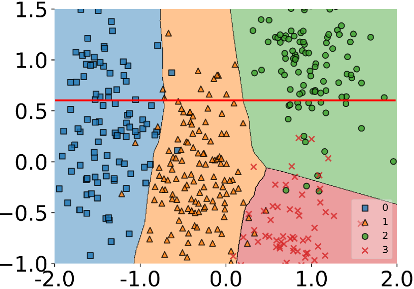
(a) Perfect Trojan

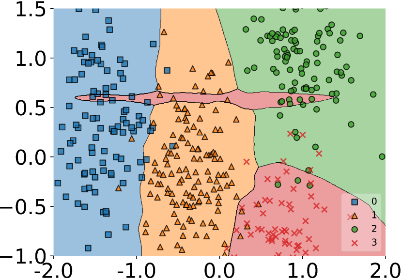
(b) Real Case: 7.5% Poisoned

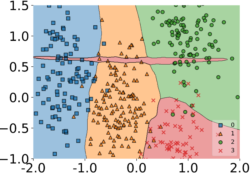
(c) Real Case: 10.0% Poisoned

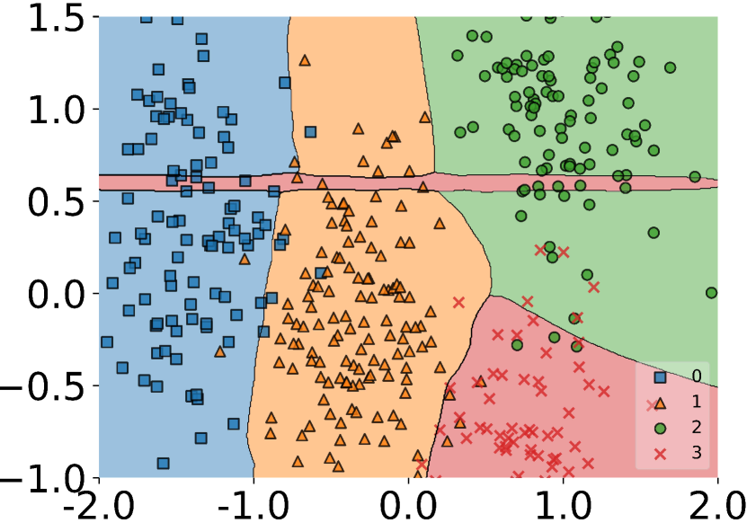
(d) Real Case: 15.0% Poisoned

Figure 4: Perfect Trojans and Relaxations on 2D Data. Each sub-figure contains test samples (dots) and the learned decision regions for different labels (in different colors) under a specific setting. The Trojan trigger is $t=(-,0.6)$, and the target label $y_{t}=3$. The red region near (-, 0.6) is the learned Trojan decision region.

To evaluate if the Trojan decision region in real-world data is the relaxation of the Trojan linear hyperplane, we visualize the decision regions of Trojaned neural networks.

Following Bai et al. [59], we visualize the decision region of neural networks on 2d data. Specifically, We visualize decision regions of compromised Multilayer Perceptrons (MLP) trained on different poisoning rates. The MLP model has 5 layers and each layer contains 100 neurons, and we use ReLU as the activation function. Similar to Bai et al. [59], the used dataset contains five isotropic Gaussian 2d blobs, in which each blob represents a class. In Figure 4, we show the complete and precise Trojan decision region (4(a)) for this model and real-world relaxations with different poisoning rates of BadNets attack (4(b), 4(c), 4(d)). Each color in the figure denotes one output label. In our experiments, we set the trigger to $t=(-,0.6)$, and the target class $y_{t}=3$ (red). Thus, the red region close to $t=(-,0.6)$ denotes the Trojan region. We observe that, with the growth of the poisoning ratio, the attacks get a higher attack success rate and become more precise, and the Trojan region also converts to the ideal one shown in 4(a). Despite such relaxations, we can also confirm that the Trojan region has a large intersection with the hyperplane and other possible triggers are around the ground truth one.

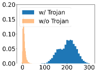
(a)

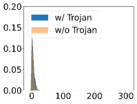
(b)

(c)

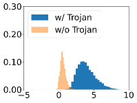
(a)

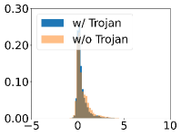
(b)

(c)

Figure 6: Comparison of Activation Values on Different Network Architectures.

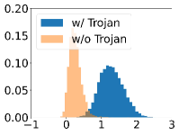
(a)

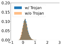
(b)

(c)

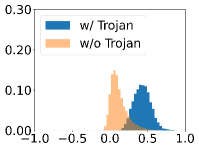
(d)

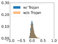
(e)

(f)

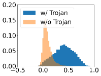
(g)

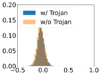
(h)

(i)

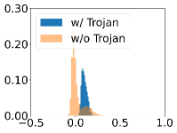
(j)

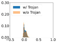
(k)

(l)

Figure 8: Comparison of Activation Values on Different CNN Layers in ResNet18 Model.

8.2 Empirical Evidence for Theorem 3.3 on Other Models

Different model architectures. To evaluate the linearity of different model architectures, we collect the activation outputs of models with different architectures (i.e., NiN and VGG16). Similar to § 3 in the main paper, we use both benign samples and compromised samples as the input of models and collect their activation outputs. The results are shown in Figure 6. The results show that compromised samples always lead to significantly higher activation values than benign samples in different models. The conclusion is consistent with the linearity theory in § 3 of the main paper and proves that our theory can generalize to different model architectures.

Different model layers: Besides the linearity on different model architectures, we also evaluate the linearity on different model layers. Figure 8 demonstrates the activation outputs of different convolutional layers (i.e., 14 to 17 layers). Note that we only show the results on 4 layers due to the space limitation.The results on other layers are similar. From the results, we observe that Trojans introduce a large set of high activation values in each layer, leading to the final linearity between input and activation output. The results are consistent with our previous analysis in § 3 of the main paper and further confirm that Trojans can introduce linearity at each layer of the DNN model.

Different activation functions. To investigate if our theory and NONE can generalize on different activation functions, we train 5 ResNet18 models on CIFAR-10 with 2 common used linear activation functions (i.e., ReLU [60], LeakyReLU [61]) and 3 non-linear activation functions (i.e., ELU [62], Tanhshrink [63] and Softplus [64]). Then we apply NONE to protect these models. We report the ASR and BA of both protected models and undefended models. The results are shown in Table 10. Overall, we find that NONE always achieves a low ASR when using different activation functions, showing the generalization of NONE on different activation functions. Even with non-linear activation functions, NONE is still effective and we suspect the reason is that even though some activation functions are non-linear, well-trained deep neural networks do fall into the "highly linear" regions. The results are also consistent with existing papers [44].

Table 10: Evaluation Results with Different Activation Functions.

Activation Function		Undefended			NONE
		BA	ASR		BA	ASR
ReLU		94.10%	100.00%		93.62%	1.07%
LeakyReLU		94.32%	100.00%		93.48%	1.24%
ELU		92.99%	99.93%		91.11%	1.46%
Tanhshrink		91.68%	99.76%		90.18%	5.11%
Softplus		92.81%	100.00%		89.91%	2.07%

8.3 Explaining DP-SGD Defense

DP-SGD [24] improves existing SGD methods by removing the noises added to poisoning training samples and shadows promising results in defending against Trojans. Here, we explain why it works. Specifically, we use the same settings with Figure 4 to train 2 compromised models with vanilla SGD and DP-SGD, and show the comparison results in Figure 9. Results show that data poisoning can successfully attack the vanilla SGD method. As a comparison, DP-SGD makes the decision region (red) much more complex, and removes the malicious “hyperplane” effects to defense against Trojans. Recently, Tursynbek et al. [65] quantitatively measured the curvature of DNN using Curvature Profile [66] and showed that models trained with DP-SGD produce more curved decision boundaries, which is consistent with our results. By doing so, DP-SGD breaks the “hyperplane” Trojans rely on and hence, removes the Trojan effects. However, this unavoidably affects the accuracy of benign samples. As shown in Figure 9, many benign samples got misclassified.

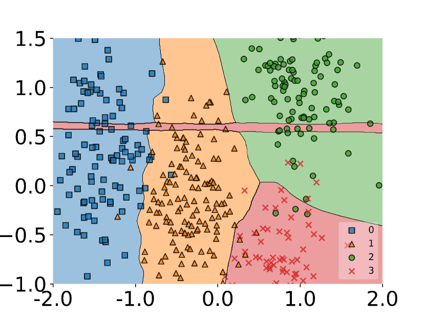
(a) SGD

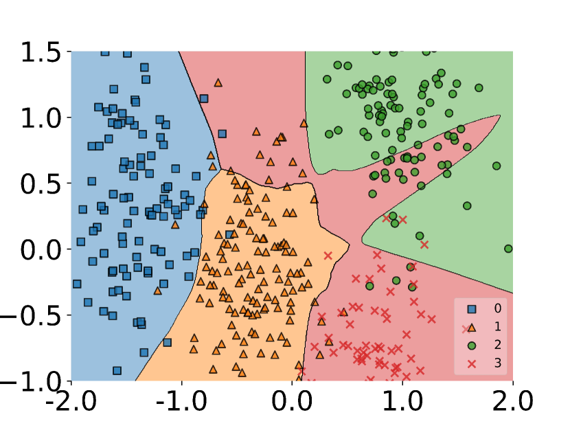
(b) DP-SGD

Figure 9: Decision Region Generated by SGD and DP-SGD.

8.4 Sample Separation

In line 13 of Algorithm 1, we separate the activation values into two clusters via Fisher’s linear discriminant analysis. In detail, we minimize the variance within clusters $\sigma_{within}$ and maximize the variance between clusters $\sigma_{between}$. The process is implemented by Jenks natural breaks optimization, which is an iterative optimization method that finds the minima/maxima of $\sigma_{within}/\sigma_{between}$. The detailed process can be found in Algorithm 2. In line 2 of Algorithm 2, it iterates all possible breaks. In lines 5 to 8, it calculates the value of $\sigma_{within}$ and $\sigma_{between}$. Lines 9 to 12 find the lowest value of $\sigma_{within}/\sigma_{between}$ and the best separation.

Algorithm 2 Jenks Natural Breaks Optimization

Input:   All Activation Values: $A_{n}$
Output:   Cluster of smaller values: $B_{n}$, Cluster of larger values: $O_{n}$

1:function Separation($A_{n}$)

2:     for break $b$ in $Breaks$ do

3:         $B_{n}^{\prime}=\{x\in A_{n}\|x\leq b\}$

4:         $O_{n}^{\prime}=\{x\in A_{n}\|x\geq b\}$

5:         $\mu_{B},\sigma_{B}=norm(B_{n}^{\prime})$

6:         $\mu_{O},\sigma_{O}=norm(O_{n}^{\prime})$

7:         $\sigma_{within}^{2}=\sigma_{B}^{2}+\sigma_{O}^{2}$

8:         $\sigma_{between}^{2}=(\mu_{B}-\mu_{O})^{2}$

9:         if  $\sigma_{within}/\sigma_{between}\leq{\rm lowest}$  then

10:              $lowest=\sigma_{within}/\sigma_{between}$

11:              $O_{n}=O_{n}^{\prime}$

12:              $B_{n}=B_{n}^{\prime}$               

8.5 Dataset Details

The overview of the dataset is shown in Table 11. Specifically, we order the datasets with their data sizes and show their dataset names, input size of each sample, the total number of samples, the number of classes and the default Trojan triggers used for generating poisoned data in each column. Among these datasets, MNIST [47] is widely used for digit classification tasks. The GTSRB [48] dataset is used for traffic sign recognition tasks in the self-driving scenario. TrojAI [51] contains the images created by compositing a synthetic traffic sign, with a random background image from the KITTI dataset [67]. Other datasets (i.e., CIFAR-10 [49] and ImageNet-10) are built for recognizing general objects (e.g., animals, plants and handicrafts). The default triggers (Figure 3 in the main paper) used for each dataset are shown in the last column of Table 11. All datasets used in the experiments are with MIT license. They are open-sourced and do not contain any personally identifiable information or offensive content.

8.6 Attack Details

We first evaluate the performances of NONE against BadNets [1] on two different settings: single target attack and label specific attack. For the single target attack, we set the label whose index is 0, 0, 1 and 1 as the target label for MNIST, CIFAR-10, GTSRB and ImageNet-10, respectively. For label specific attack, the target label of each sample is the label whose index is (the label index of this sample plus 1)%(the number of classes in the dataset). Then, we evaluate the defense against the label-consistent attack [11] and the natural Trojan attack [8]. We use the same implementation and parameters in original papers to achieve these attacks and compare NONE with other defense methods. Notice that for the label-consistent attack, the official github repository only provides poisoned CIFAR-10 datasets, and the code for training GAN and generating poisoned samples are not released. Therefore, we only evaluate NONE on CIFAR-10. For defending against the hidden trigger Trojan attack [56], we follow the parameter settings in original paper and use a pair of image categories (i.e., randomly selected from ImageNet dataset in the previous work [56]) for testing.

Table 11: Overview of Datasets.

Name	Input Size	Samples	Classes	Trigger
MNIST	28*28*1	60000	10	Single Pixel
GTSRB	32*32*3	39209	43	Static
CIFAR-10	32*32*3	50000	10	Dynamic
ImageNet-10	224*224*3	9469	10	Watermark
TrojAI	224*224*3	125000	5-25	Natural Trojans

8.7 Resistance to More Attacks

In this section, we evaluate the resistance of NONE to more attacks. Four state-of-the-art poisoning based Trojan attacks (WaNet [68], SIG attack [69], Filter attack [8] and Blend attack [10]) are included in the experiments. The dataset and the network used are CIFAR-10 and ResNet18. We report the BA and ASR of undefended model, and the model trained with NAD [38], ABL [9] and NONE. Results in Table 12 demonstrates NONE has better performance than baseline methods (i.e., NAD and ABL). On average, NONE has 0.98% ASR and 92.52% BA. The results indicate that our method is resistance to various Trojan attacks.

Table 12: Results on More Attacks.

Dataset	Network	Attack		Undefended			NAD			ABL			NONE
				BA	ASR		BA	ASR		BA	ASR		BA	ASR
CIFAR-10	ResNet18	WaNet		94.39%	96.71%		88.81%	1.17%		90.79%	2.68%		92.24%	0.69%
		SIG		94.34%	99.08%		88.26%	1.42%		91.44%	1.29%		93.79%	1.08%
		Filter		91.08%	99.34%		87.91%	4.38%		88.46%	2.24%		89.87%	1.20%
		Blend		94.62%	99.86%		88.24%	1.58%		92.72%	1.70%		94.21%	0.93%

8.8 Sensitivity to Configurable Parameters

NONE has a few configurable parameters that may affect its performance: learning rate in training, resetting fraction, number of neurons in each layer used to detect malicious samples (selection threshold) and different thresholds used for the identification of compromised neurons. We vary the configurable parameters in NONE independently and evaluate the impact of each. The setting of dataset, models and attack type is the same as evaluation in § 5.3 of the main paper. We use 5% poisoning rate, 3*3 trigger size as the default attack setting.

Learning rate. Learning rate usually affects the accuracy and convergence speed of the model during the training process. To understand how the learning rate impacts the model deployed with NONE, we choose learning rates from 0.01 to 0.00001 and then measure the BA and ASR of models using different learning rates in the training process. The results are shown in Figure 10.

Overall, as shown in 10(a), using a larger learning rate makes the convergence process faster and the BA lower, except for using the learning rate 0.01. This is because using a larger learning rate can update the weights quickly, but a too large learning rate makes it difficult to find the local optimum and decrease the BA.

In addition, in 10(b), we find that the final ASR is decreased with the decrease of learning rate after the model is converged. Using learning rate 0.00001 finally achieves the lowest ASR. The reason is that increasing the learning rate tends to make the model skip the local optimal value and get a more likely worse value.

Therefore, combining the results in these 2 subfigures, we choose the learning rate 0.001 as the default setting in § 5.2 because using 0.001 achieves the best BA and ASR. The epoch number is set to 5 because ASR is not decreased after 5 epochs and the BA is already good.

Resetting fraction. Resetting fraction measures the number of neurons that are reset by NONE. Specifically, NONE first sorts the probabilities that the neuron has activation values larger than 0 and then resets the neurons whose probabilities is in top $r_{1}\%$ in each layer. Using a smaller resetting fraction makes NONE to detect compromised neurons more conservatively (only labeling and resetting the most likely compromised neurons). To measure the effect of resetting fraction on defense performance of NONE, we obtain the BA and ASR of models at different resetting fractions from 0.5% to 15%. The results are shown in Figure 11, where the legend shows different resetting fraction values.

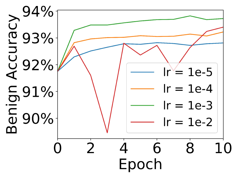
(a) Benign Accuracy

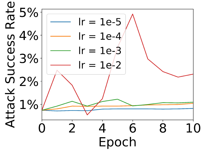
(b) Attack Success Rate

Figure 10: Evaluation Results with Different Learning Rates.

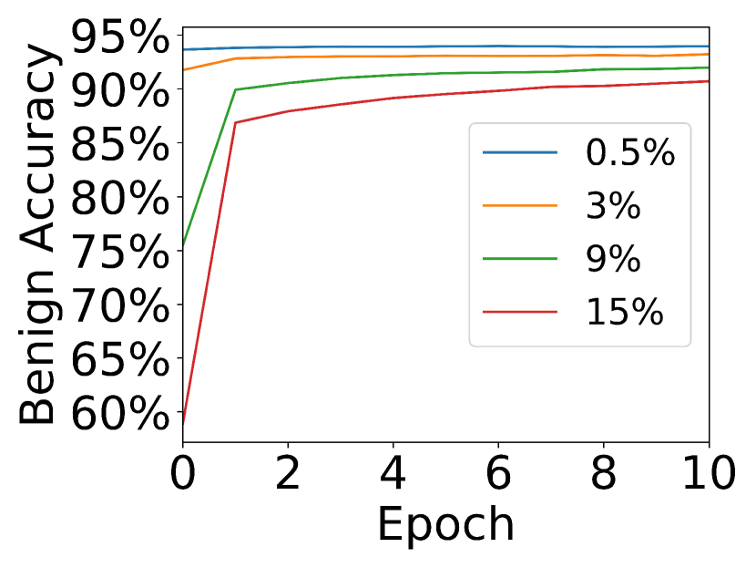
(a) Benign Accuracy

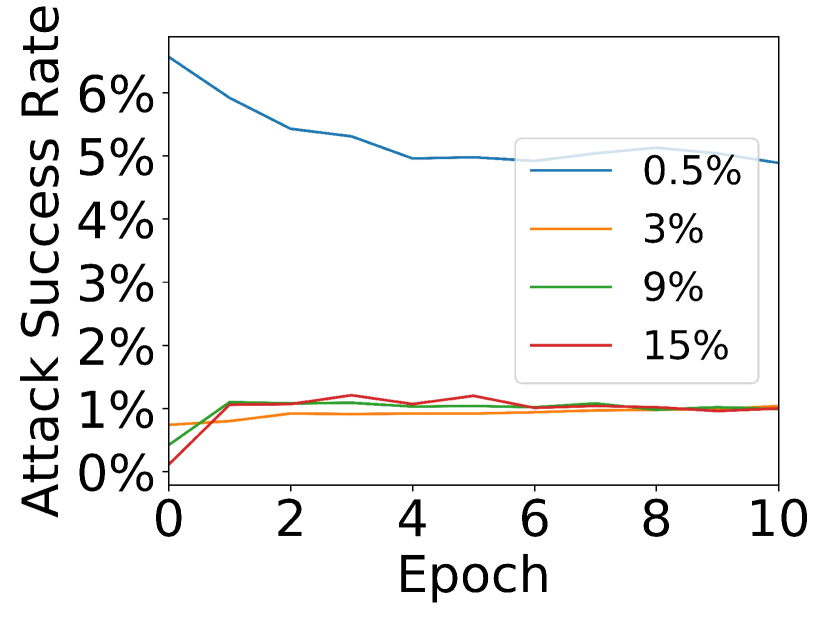
(b) Attack Success Rate

Figure 11: Evaluation Results with Different Resetting Fractions.

From the results in 11(a), it is obvious that when we use a larger resetting fraction and reset more neurons, the final BA is lower. The reason is that after we reset neurons, some good features learned by the model are lost, which decreases the final BA. When we reset more neurons (i.e., using a larger resetting fraction), the model loses more high quality features and decreases more BA. Therefore, to avoid losing too much BA, the resetting fraction is recommended to be small.

Table 13: Results on Different Selection Thresholds.

Number of Neurons	Single Target Attack			Label Specific Attack
	BA	ASR		BA	ASR
top 1	93.11%	1.03%		93.31%	0.96%
top 0.5%	93.10%	1.07%		93.32%	0.96%
top 1%	93.13%	1.07%		93.37%	0.95%
top 10%	93.11%	1.06%		93.29%	1.04%
top 30%	93.14%	1.04%		93.26%	41.07%
top 50%	93.08%	1.04%		93.18%	60.12%
top 100%	93.05%	1.07%		93.14%	71.78%

Table 14: Results on Different $\lambda_{l}$ and $\lambda_{h}$.

$\lambda_{h}$	BA	ASR	$\lambda_{l}$	BA	ASR
0.3	93.22%	1.07%	0.1	93.18%	1.13%
0.5	93.05%	1.14%	0.3	93.08%	0.99%
0.7	93.13%	1.11%	0.5	93.18%	1.11%
0.9	93.12%	1.11%	0.7	93.11%	1.03%

Furthermore, in 11(b), we find that different resetting fractions do not affect the ASR of models after a certain threshold (i.e., 3%). Because when the resetting fraction is large, NONE can successfully detect almost all compromised neurons. Increasing the resetting fraction does not help NONE to detect more compromised neurons.

Based on the above conclusions, we set the default resetting fraction as 3% because using resetting fraction 3% requires changing fewer neurons, achieving high BA and low ASR.

Selection threshold. When detecting poisoning samples, we only use the neurons whose compromised values are larger than the values of a portion of neurons in the same layer and we call this portion as selection threshold. To fully understand the impact of this threshold, we vary the threshold from 1 neuron to 100% neurons in the dataset and collect the corresponding BA and ASR under different attack settings. We test the single target BadNets attack and the label specific BadNets attack. We then show the results in Table 13, where the first column shows the threshold and the following columns show the results against the BadNets.

As the results show, when we increase the selection threshold, the ASR of the label specific BadNets attack significantly increases when the threshold is larger than 10%. This is because only a few neurons in the model are compromised. If the selection threshold is larger than the number of compromised neurons, NONE chooses many benign neurons to identify whether a sample is malicious or not, which introduces more noise and reduces the detection accuracy because benign neurons are not sensitive to Trojan behavior. Furthermore, the label specific BadNets attack specifies many different labels as target labels, making the attack stealthy and detecting the attack more difficult. Therefore, with the increase of the selection threshold, the defense performance becomes worse.

However, we observe that the ASR of the single target standard Trojan attack is not correlated with the selection threshold, showing the robustness of NONE to selection threshold against the single target Trojan attack. This is due to the fact that the single target BadNets attack only focuses on one label, making the malicious behavior more obvious, thus reducing the impact of introduced noise and still achieving a low ASR.

For the BA, we find that the BA against both the single target BadNets attack and the label specific BadNets attack is stable. Although using a lower selection threshold may allow NONE to filter out malicious samples conservatively (i.e., only use the most likely compromised neurons to detect malicious samples), enabling NONE to train the model on most of the data and achieve good BA results. Choosing a higher selection threshold does not decrease the BA significantly. Because considering there are a large number of benign samples in the dataset, even a higher selection threshold introduces more benign neurons (i.e., noise) to identify malicious samples and reduces the number of benign samples for finetuning, NONE still has enough benign samples for training and achieves similar BA results as using low selection thresholds.

Therefore, considering both BA and ASR, we set the selection threshold as 10% to avoid the ASR increasing significantly.

Parameters in compromised neurons identification. As mentioned in § 4 of the main paper, we use an alternative implementation to evaluate our design. We first obtain two clusters of samples according to their final layer probability outputs (the value in the probability vector). Subsequently, we classify the samples whose probability values are lower than a threshold $\lambda_{l}$ to the first cluster (i.e., low confidence samples) and classify the samples whose probability values are higher than $\lambda_{h}$ to the second cluster (i.e., low confidence samples). Then, we use the gap between two clusters to measure the linearity of each neuron. If a neuron has high linearity (i.e., top $r_{1}$ in a layer), then we consider it as a compromised neuron. In this process, $\lambda_{h}$ and $\lambda_{l}$ determine the selection of the high confidence

Table 15: Comparisons on Efficiency.

Method	Runtime	Overhead
Native training	2898.4s	N/A
AC	4459.7s	53.86%
ABL	3197.4s	10.31%
NONE	3149.7s	8.60%

samples and the low confidence samples that affect the defense performance of NONE. Therefore, to fully understand the impacts of them, We vary $\lambda_{h}$ and $\lambda_{l}$ values, and obtain the corresponding ASR and BA. By default, we use $\lambda_{h}$ as 0.9 and $\lambda_{l}$ to be 0.1 when the other parameter is changing.

Table 14 shows the results with different $\lambda_{h}$ and $\lambda_{l}$ settings. The results indicate that there is no obvious correlation between the performance of NONE and parameters (i.e., $\lambda_{l}$ and $\lambda_{h}$). As the results show, the ASR of models is always around 1.11% under different parameter settings. And the difference between the highest BA and the lowest BA is 0.17% which is quite small. Therefore, NONE is not sensitive to $\lambda_{l}$ and $\lambda_{h}$, which improves the usability of NONE.

8.9 Efficiency

We compare the total training time of native training, AC [22], ABL [9], and our method on the CIFAR-10 dataset with ResNet18. The results are shown in Table 15. The epoch number (i.e., 100) and batch size (i.e., 128) for different methods are the same. The ASR and BA are consistent with results in Table 1. We run each method with five trails and report the average time. All methods are run on the same device specified in § 5 of the main paper. Thus, our method is efficient.

Figure 12: Trojan Inputs with Large Triggers.

8.10 Adaptive Attack

In this paper, we assume that attackers can poison the training data but have no control over the training procedure, e.g., the training algorithm, code, and hardware. This is consistent with existing work [24, 22, 9, 58]. It is hard for attackers to conduct adaptive attacks under the threat model because they can not directly control the training of the model, instead, NONE will be in charge of the training process. Therefore, we relax the threat model and consider the adaptive attacker in a code-poisoning attack [57], which requires extra capability from the adversary, i.e., modifying the training procedure.

In the considered adaptive code-poisoning attacks, the adversary goal is to train a Trojaned model with low linearity and try to evade the defense of NONE. However, under our threat model, the adversary can only poison the data but cannot modify the training process of NONE, which makes reducing the model’s internal linearity almost impossible. Therefore, we relax the threat model for attackers and allow the attacker to control the training process of the model. We also assume the defender can access both the training data and the trained model. The defender tries to use NONE to eliminate Trojans injected in the model trained by the attacker.

Then, we design an adaptive loss that minimizes the activation difference between benign samples and corresponding Trojan samples to achieve attack goals. The adaptive loss is defined in Eq. 9, where $\bm{x}$ is benign sample and $\tilde{\bm{x}}$ is the corresponding Trojan sample (i.e., the sample obtained by pasting trigger on $\bm{x}$).

$$\mathcal{L}\left(F_{\theta}(\bm{x}),y\right)+\mathcal{L}\left(F_{\theta}(\tilde{\bm{x}}),y_{t}\right)+\alpha\sum(I_{i}({\bm{x}})-I_{i}(\tilde{\bm{x}}))^{2}$$ (9)

$y$ and $y_{t}$ are the label of benign sample $\bm{x}$ and target label respectively. $F_{\theta}$ donates the final prediction of the model. $\mathcal{L}$ means the Cross-Entropy criterion. Meanwhile, $I_{i}$ is the feature on the i-th layer, and $\alpha$ is the weight that controls the influence of the third loss item. By design, the loss function minimizes the distance between activation values of benign samples and the corresponding Trojan samples, making the Trojan decision region more curve and complex. Trojan models trained with the adaptive loss should have low linearity and may evade the detection of NONE.

Table 16: Adaptive Attack.

$\alpha$		Undefended			NONE
		BA	ASR		BA	ASR
1e-4		90.06%	100.00%		88.48%	67.89%
1e-3		89.53%	99.97%		87.92%	76.78%
1e-2		89.03%	99.91%		86.50%	86.20%
1e-1		88.72%	99.98%		85.71%	94.92%

To measure whether the adaptive attack works, we first train a benign model and then fine-tune that model using adaptive loss when attackers use poisoned data to attack the model. The Trojan trigger we use in the attack is the watermarking trigger and the model is VGG16. The results are shown in  Table 16. The results show that NONE does not always achieve good defense against adaptive attacks. For example, when $\alpha=1e-1$, the BA and the ASR of NONE is 85.71% and 94.92%, respectively. However, the BA and ASR of the model trained with NONE are lower than that of the undefended model, showing that NONE helps in training a better model.

8.11 Comparison with DBD

Besides existing defenses compared in § 5.2 (i.e., DP-SGD [24], NAD [38], AC [22], ABL [9]), we also compare NONE with another training time defense DBD [58]. DBD defends backdoor attacks by decoupling the end-to-end training process into three stages, i.e., self-supervised learning for the backdoor, supervised training for the fully-connected layers, and semi-supervised fine-tuning of the whole model. We use six different attacks (i.e., BadNets [1], Label-consistent [11], Blend [10], SIG [69], Filter [8], WaNet [68]) and the CIFAR-10 dataset. We report the BA and ASR of the native training, DBD, and NONE in Table 17. The average runtime of DBD and NONE are 18,988.4s and 3,149.7s, respectively. For all attacks, our method achieves higher BA than DBD. In addition, in five of six attacks, the ASR of NONE is lower than that of DBD. The results show that our method is more effective and efficient than DBD.

Table 17: Comparison to DBD [58].

Attack		Undefended			DBD			NONE
		BA	ASR		BA	ASR		BA	ASR
BadNets		94.10%	100.00%		91.24%	1.25%		93.62%	1.07%
Label-consistent		94.73%	83.42%		91.08%	1.87%		94.01%	2.14%
Blend		94.62%	99.86%		92.03%	1.96%		94.21%	0.93%
SIG		94.34%	99.08%		91.55%	1.51%		93.79%	1.08%
Filter		91.08%	99.34%		88.75%	1.42%		89.87%	1.20%
WaNet		94.39%	96.71%		90.98%	0.95%		92.24%	0.69%

8.12 Comparison to More Defenses on Natural Trojan

Besides the results of comparison to DP-SGD on natural Trojan (§ 5.2), we compare NONE with more training-time defenses (i.e., DP-SGD [24], NAD [38], AC [22], ABL [9], DBD [58]) on natural Trojan [8]. The dataset used here is CIFAR-10, and DNNs are NiN and VGG16. As shown in Table 18, the average ASR of NONE is 33.07%, 2.41 times lower than the undefended model. However, the average ASR of DP-SGD, NAD, AC, ABL, and DBD are 75.4%, 80.43%, 77.45%, 79.32%, 77.99%, respectively. The results demonstrate all existing methods have high ASR when facing natural backdoors, while our method can reduce the ASR significantly.

Table 18: Comparisons to More Defenses on Natural Trojan.

Network		Undefended			DP-SGD			NAD			AC			ABL			DBD			NONE
		BA	ASR		BA	ASR		BA	ASR		BA	ASR		BA	ASR		BA	ASR		BA	ASR
NiN		91.02%	87.62%		39.19%	87.22%		80.75%	88.10%		83.85%	88.28%		86.28%	86.33%		86.27%	87.54%		86.94%	34.21%
VGG16		90.78%	71.88%		53.40%	63.58%		85.20%	72.76%		85.69%	66.67%		86.46%	72.32%		86.38%	68.45%		81.83%	31.49%

8.13 Generalization to Larger Models

To study NONE’s generalization to larger models, we report its BA and ASR on ResNet34 [53] and Wide-ResNet-16 (WRN16) [70]. The results of two baseline methods (i.e., NAD [38] and ABL [9]) are also reported. The dataset used is CIFAR-10. The runtime overhead of NONE on ResNet34 and WRN16 are 10.15% and 9.73%, respectively. For both two models, NONE achieves higher BA and lower ASR than NAD and ABL. For ResNet34, the BA of NONE is 2.47% and 2.84% higher than NAD and ABL. The ASR of NONE for ResNet34 is also 1.45% and 0.19% lower than that of NAD and ABL. The results show that our method is scalable to larger models.

8.14 Generalization to Larger Datasets

To evaluate the generalization of NONE to larger datasets, we report the performance (i.e., BA, ASR, and Runtime) of native training and NONE on a ImageNet subset (200 classes with 100k images for training and 10k images for testing) from Li et al. [71]. The results can be found in Table 20. NONE achieves low ASR (i.e., 1.98%, 50.32 times lower than Native Training) with a high BA (i.e., 1.66% lower than native training). In addition, the overheads compared with native training is 13.86%.

Table 19: Generalization to Larger Models.

Networks		NAD			ABL			Ours
		BA	ASR		BA	ASR		BA	ASR
ResNet34		90.54%	2.67%		90.17%	1.41%		93.01%	1.22%
WRN16		86.73%	5.96%		84.70%	5.04%		88.28%	3.88%

Table 20: Generalization to Larger Datasets.

Method	BA	ASR	Runtime
Native Training	85.12%	99.65%	23.8h
NONE	83.46%	1.98%	27.1h

References

- Gu et al. [2019] Tianyu Gu, Brendan Dolan-Gavitt, and Siddharth Garg. Badnets: Identifying vulnerabilities in the machine learning model supply chain. IEEE Access, 2019.
- Jia et al. [2022] Jinyuan Jia, Yupei Liu, and Neil Zhenqiang Gong. Badencoder: Backdoor attacks to pre-trained encoders in self-supervised learning. 2022 IEEE Symposium on Security and Privacy (SP), 2022.
- Carlini and Terzis [2021] Nicholas Carlini and Andreas Terzis. Poisoning and backdooring contrastive learning. In International Conference on Learning Representations, 2021.
- Wang et al. [2021] Lun Wang, Zaynah Javed, Xian Wu, Wenbo Guo, Xinyu Xing, and Dawn Song. Backdoorl: Backdoor attack against competitive reinforcement learning. International Joint Conference on Artificial Intelligence (IJCAI), 2021.
- Bagdasaryan and Shmatikov [2021a] Eugene Bagdasaryan and Vitaly Shmatikov. Spinning sequence-to-sequence models with meta-backdoors. arXiv preprint arXiv:2107.10443, 2021a.
- Chen et al. [2021] Xiaoyi Chen, Ahmed Salem, Dingfan Chen, Michael Backes, Shiqing Ma, Qingni Shen, Zhonghai Wu, and Yang Zhang. Badnl: Backdoor attacks against nlp models with semantic-preserving improvements. In Annual Computer Security Applications Conference, pages 554–569, 2021.
- Xie et al. [2019] Chulin Xie, Keli Huang, Pin-Yu Chen, and Bo Li. Dba: Distributed backdoor attacks against federated learning. In International Conference on Learning Representations, 2019.
- Liu et al. [2019] Yingqi Liu, Wen-Chuan Lee, Guanhong Tao, Shiqing Ma, Yousra Aafer, and Xiangyu Zhang. Abs: Scanning neural networks for back-doors by artificial brain stimulation. In Proceedings of the 2019 ACM SIGSAC Conference on Computer and Communications Security, pages 1265–1282, 2019.
- Li et al. [2021a] Yige Li, Xixiang Lyu, Nodens Koren, Lingjuan Lyu, Bo Li, and Xingjun Ma. Anti-backdoor learning: Training clean models on poisoned data. Advances in Neural Information Processing Systems, 34, 2021a.
- Chen et al. [2017] Xinyun Chen, Chang Liu, Bo Li, Kimberly Lu, and Dawn Song. Targeted backdoor attacks on deep learning systems using data poisoning. arXiv preprint arXiv:1712.05526, 2017.
- Turner et al. [2019] Alexander Turner, Dimitris Tsipras, and Aleksander Madry. Label-consistent backdoor attacks. arXiv preprint arXiv:1912.02771, 2019.
- Salem et al. [2022] Ahmed Salem, Rui Wen, Michael Backes, Shiqing Ma, and Yang Zhang. Dynamic backdoor attacks against machine learning models. In 2022 IEEE 7th European Symposium on Security and Privacy (EuroS&P), pages 703–718. IEEE, 2022.
- Nguyen and Tran [2020] Anh Nguyen and Anh Tran. Input-aware dynamic backdoor attack. Advances in Neural Information Processing Systems 30. Pre-proceedings, 2020.
- Tang et al. [2021] Di Tang, XiaoFeng Wang, Haixu Tang, and Kehuan Zhang. Demon in the variant: Statistical analysis of dnns for robust backdoor contamination detection. In 30th USENIX Security Symposium (USENIX Security 21), 2021.
- Saha et al. [2022] Aniruddha Saha, Ajinkya Tejankar, Soroush Abbasi Koohpayegani, and Hamed Pirsiavash. Backdoor attacks on self-supervised learning. In Proceedings of the IEEE/CVF Conference on Computer Vision and Pattern Recognition, pages 13337–13346, 2022.
- Li et al. [2021b] Yiming Li, Yanjie Li, Yalei Lv, Yong Jiang, and Shu-Tao Xia. Hidden backdoor attack against semantic segmentation models. arXiv preprint arXiv:2103.04038, 2021b.
- Cheng et al. [2021] Siyuan Cheng, Yingqi Liu, Shiqing Ma, and Xiangyu Zhang. Deep feature space trojan attack of neural networks by controlled detoxification. In Proceedings of the AAAI Conference on Artificial Intelligence, volume 35, pages 1148–1156, 2021.
- Wang et al. [2022] Zhenting Wang, Juan Zhai, and Shiqing Ma. Bppattack: Stealthy and efficient trojan attacks against deep neural networks via image quantization and contrastive adversarial learning. In Proceedings of the IEEE/CVF Conference on Computer Vision and Pattern Recognition, pages 15074–15084, 2022.
- Lin et al. [2014] Min Lin, Qiang Chen, and Shuicheng Yan. Network in network. International Conference on Learning Representations, 2014.
- Zhao et al. [2021] Shihao Zhao, Xingjun Ma, Yisen Wang, James Bailey, Bo Li, and Yu-Gang Jiang. What do deep nets learn? class-wise patterns revealed in the input space. arXiv preprint arXiv:2101.06898, 2021.
- Tran et al. [2018] Brandon Tran, Jerry Li, and Aleksander Madry. Spectral signatures in backdoor attacks. Advances in neural information processing systems, 31, 2018.
- Chen et al. [2019] Bryant Chen, Wilka Carvalho, Nathalie Baracaldo, Heiko Ludwig, Benjamin Edwards, Taesung Lee, Ian Molloy, and Biplav Srivastava. Detecting backdoor attacks on deep neural networks by activation clustering. SafeAI@AAAI, 2019.
- Du et al. [2020] Min Du, Ruoxi Jia, and Dawn Song. Robust anomaly detection and backdoor attack detection via differential privacy. International Conference on Learning Representations, 2020.
- Hong et al. [2020] Sanghyun Hong, Varun Chandrasekaran, Yiğitcan Kaya, Tudor Dumitraş, and Nicolas Papernot. On the effectiveness of mitigating data poisoning attacks with gradient shaping. arXiv preprint arXiv:2002.11497, 2020.
- Abadi et al. [2016] Martin Abadi, Andy Chu, Ian Goodfellow, H Brendan McMahan, Ilya Mironov, Kunal Talwar, and Li Zhang. Deep learning with differential privacy. In Proceedings of the 2016 ACM SIGSAC conference on computer and communications security, pages 308–318, 2016.
- Wang et al. [2019] Bolun Wang, Yuanshun Yao, Shawn Shan, Huiying Li, Bimal Viswanath, Haitao Zheng, and Ben Y Zhao. Neural cleanse: Identifying and mitigating backdoor attacks in neural networks. In 2019 IEEE Symposium on Security and Privacy (SP), pages 707–723. IEEE, 2019.
- Xu et al. [2021] Xiaojun Xu, Qi Wang, Huichen Li, Nikita Borisov, Carl A Gunter, and Bo Li. Detecting ai trojans using meta neural analysis. In 2021 IEEE Symposium on Security and Privacy (SP), pages 103–120. IEEE, 2021.
- Kolouri et al. [2020] Soheil Kolouri, Aniruddha Saha, Hamed Pirsiavash, and Heiko Hoffmann. Universal litmus patterns: Revealing backdoor attacks in cnns. In Proceedings of the IEEE/CVF Conference on Computer Vision and Pattern Recognition, pages 301–310, 2020.
- Huang et al. [2020] Shanjiaoyang Huang, Weiqi Peng, Zhiwei Jia, and Zhuowen Tu. One-pixel signature: Characterizing cnn models for backdoor detection. In European Conference on Computer Vision, pages 326–341. Springer, 2020.
- Guo et al. [2020] Wenbo Guo, Lun Wang, Xinyu Xing, Min Du, and Dawn Song. Tabor: A highly accurate approach to inspecting and restoring trojan backdoors in ai systems. IEEE International Conference on Data Mining (ICDM),, 2020.
- Shen et al. [2021] Guangyu Shen, Yingqi Liu, Guanhong Tao, Shengwei An, Qiuling Xu, Siyuan Cheng, Shiqing Ma, and Xiangyu Zhang. Backdoor scanning for deep neural networks through k-arm optimization. In International Conference on Machine Learning, pages 9525–9536. PMLR, 2021.
- Liu et al. [2022a] Yingqi Liu, Guangyu Shen, Guanhong Tao, Zhenting Wang, Shiqing Ma, and Xiangyu Zhang. Complex backdoor detection by symmetric feature differencing. In Proceedings of the IEEE/CVF Conference on Computer Vision and Pattern Recognition, pages 15003–15013, 2022a.
- Tao et al. [2022] Guanhong Tao, Guangyu Shen, Yingqi Liu, Shengwei An, Qiuling Xu, Shiqing Ma, Pan Li, and Xiangyu Zhang. Better trigger inversion optimization in backdoor scanning. In Proceedings of the IEEE/CVF Conference on Computer Vision and Pattern Recognition, pages 13368–13378, 2022.
- Liu et al. [2022b] Yingqi Liu, Guangyu Shen, Guanhong Tao, Shengwei An, Shiqing Ma, and Xiangyu Zhang. Piccolo: Exposing complex backdoors in nlp transformer models. In 2022 IEEE Symposium on Security and Privacy (SP), pages 1561–1561. IEEE Computer Society, 2022b.
- Shen et al. [2022] Guangyu Shen, Yingqi Liu, Guanhong Tao, Qiuling Xu, Zhuo Zhang, Shengwei An, Shiqing Ma, and Xiangyu Zhang. Constrained optimization with dynamic bound-scaling for effective nlpbackdoor defense. 2022.
- Liu et al. [2018] Kang Liu, Brendan Dolan-Gavitt, and Siddharth Garg. Fine-pruning: Defending against backdooring attacks on deep neural networks. In International Symposium on Research in Attacks, Intrusions, and Defenses, pages 273–294. Springer, 2018.
- Zhao et al. [2020] Pu Zhao, Pin-Yu Chen, Payel Das, Karthikeyan Natesan Ramamurthy, and Xue Lin. Bridging mode connectivity in loss landscapes and adversarial robustness. arXiv preprint arXiv:2005.00060, 2020.
- Li et al. [2021c] Yige Li, Nodens Koren, Lingjuan Lyu, Xixiang Lyu, Bo Li, and Xingjun Ma. Neural attention distillation: Erasing backdoor triggers from deep neural networks. International Conference on Learning Representations, 2021c.
- Wu and Wang [2021] Dongxian Wu and Yisen Wang. Adversarial neuron pruning purifies backdoored deep models. Advances in Neural Information Processing Systems, 34, 2021.
- Zeng et al. [2022] Yi Zeng, Si Chen, Won Park, Zhuoqing Mao, Ming Jin, and Ruoxi Jia. Adversarial unlearning of backdoors via implicit hypergradient. In International Conference on Learning Representations, 2022.
- Gao et al. [2019] Yansong Gao, Change Xu, Derui Wang, Shiping Chen, Damith C Ranasinghe, and Surya Nepal. Strip: A defence against trojan attacks on deep neural networks. In Proceedings of the 35th Annual Computer Security Applications Conference, pages 113–125, 2019.
- Chou et al. [2020] Edward Chou, Florian Tramèr, and Giancarlo Pellegrino. Sentinet: Detecting localized universal attacks against deep learning systems. In 2020 IEEE Security and Privacy Workshops (SPW), pages 48–54. IEEE, 2020.
- Ma and Liu [2019] Shiqing Ma and Yingqi Liu. Nic: Detecting adversarial samples with neural network invariant checking. In Proceedings of the 26th network and distributed system security symposium (NDSS 2019), 2019.
- Goodfellow et al. [2015] Ian J Goodfellow, Jonathon Shlens, and Christian Szegedy. Explaining and harnessing adversarial examples. International Conference on Learning Representations, 2015.
- Tang et al. [2020] Ruixiang Tang, Mengnan Du, Ninghao Liu, Fan Yang, and Xia Hu. An embarrassingly simple approach for trojan attack in deep neural networks. In Proceedings of the 26th ACM SIGKDD International Conference on Knowledge Discovery & Data Mining, pages 218–228, 2020.
- Otsu [1979] Nobuyuki Otsu. A threshold selection method from gray-level histograms. IEEE transactions on systems, man, and cybernetics, 9(1):62–66, 1979.
- LeCun et al. [1998] Yann LeCun, Léon Bottou, Yoshua Bengio, and Patrick Haffner. Gradient-based learning applied to document recognition. Proceedings of the IEEE, 86(11):2278–2324, 1998.
- Stallkamp et al. [2012] Johannes Stallkamp, Marc Schlipsing, Jan Salmen, and Christian Igel. Man vs. computer: Benchmarking machine learning algorithms for traffic sign recognition. Neural networks, 32:323–332, 2012.
- Krizhevsky et al. [2009] Alex Krizhevsky, Geoffrey Hinton, et al. Learning multiple layers of features from tiny images. 2009.
- Krizhevsky et al. [2012] Alex Krizhevsky, Ilya Sutskever, and Geoffrey E Hinton. Imagenet classification with deep convolutional neural networks. Advances in neural information processing systems, 25:1097–1105, 2012.
- Karra et al. [2020] Kiran Karra, Chace Ashcraft, and Neil Fendley. The trojai software framework: An opensource tool for embedding trojans into deep learning models. arXiv preprint arXiv:2003.07233, 2020.
- Simonyan and Zisserman [2014] Karen Simonyan and Andrew Zisserman. Very deep convolutional networks for large-scale image recognition. arXiv preprint arXiv:1409.1556, 2014.
- He et al. [2016] Kaiming He, Xiangyu Zhang, Shaoqing Ren, and Jian Sun. Deep residual learning for image recognition. In Proceedings of the IEEE conference on computer vision and pattern recognition, pages 770–778, 2016.
- Veldanda et al. [2020] Akshaj Kumar Veldanda, Kang Liu, Benjamin Tan, Prashanth Krishnamurthy, Farshad Khorrami, Ramesh Karri, Brendan Dolan-Gavitt, and Siddharth Garg. Nnoculation: broad spectrum and targeted treatment of backdoored dnns. arXiv preprint arXiv:2002.08313, 2020.
- Doan et al. [2020] Bao Gia Doan, Ehsan Abbasnejad, and Damith C Ranasinghe. Februus: Input purification defense against trojan attacks on deep neural network systems. In Annual Computer Security Applications Conference, pages 897–912, 2020.
- Saha et al. [2020] Aniruddha Saha, Akshayvarun Subramanya, and Hamed Pirsiavash. Hidden trigger backdoor attacks. In Proceedings of the AAAI Conference on Artificial Intelligence, volume 34, pages 11957–11965, 2020.
- Bagdasaryan and Shmatikov [2021b] Eugene Bagdasaryan and Vitaly Shmatikov. Blind backdoors in deep learning models. In 30th USENIX Security Symposium (USENIX Security 21), pages 1505–1521, 2021b.
- Huang et al. [2022] Kunzhe Huang, Yiming Li, Baoyuan Wu, Zhan Qin, and Kui Ren. Backdoor defense via decoupling the training process. International Conference on Learning Representations, 2022.
- Bai et al. [2021] Jiawang Bai, Baoyuan Wu, Yong Zhang, Yiming Li, Zhifeng Li, and Shu-Tao Xia. Targeted attack against deep neural networks via flipping limited weight bits. In International Conference on Learning Representations, 2021.
- Nair and Hinton [2010] Vinod Nair and Geoffrey E Hinton. Rectified linear units improve restricted boltzmann machines. In Icml, 2010.
- Maas et al. [2013] Andrew L Maas, Awni Y Hannun, and Andrew Y Ng. Rectifier nonlinearities improve neural network acoustic models. In Proc. icml, volume 30, page 3. Citeseer, 2013.
- Clevert et al. [2015] Djork-Arné Clevert, Thomas Unterthiner, and Sepp Hochreiter. Fast and accurate deep network learning by exponential linear units (elus). arXiv preprint arXiv:1511.07289, 2015.
- [63] Tanhshrink. https://pytorch.org/docs/stable/generated/torch.nn.Tanhshrink.html.
- Zheng et al. [2015] Hao Zheng, Zhanlei Yang, Wenju Liu, Jizhong Liang, and Yanpeng Li. Improving deep neural networks using softplus units. In 2015 International Joint Conference on Neural Networks (IJCNN), pages 1–4. IEEE, 2015.
- Tursynbek et al. [2020] Nurislam Tursynbek, Aleksandr Petiushko, and Ivan Oseledets. Robustness threats of differential privacy. arXiv preprint arXiv:2012.07828, 2020.
- Moosavi-Dezfooli et al. [2019] Seyed-Mohsen Moosavi-Dezfooli, Alhussein Fawzi, Jonathan Uesato, and Pascal Frossard. Robustness via curvature regularization, and vice versa. In Proceedings of the IEEE/CVF Conference on Computer Vision and Pattern Recognition, pages 9078–9086, 2019.
- Geiger et al. [2013] Andreas Geiger, Philip Lenz, Christoph Stiller, and Raquel Urtasun. Vision meets robotics: The kitti dataset. The International Journal of Robotics Research, 32(11):1231–1237, 2013.
- Nguyen and Tran [2021] Tuan Anh Nguyen and Anh Tuan Tran. Wanet-imperceptible warping-based backdoor attack. In International Conference on Learning Representations, 2021.
- Barni et al. [2019] Mauro Barni, Kassem Kallas, and Benedetta Tondi. A new backdoor attack in cnns by training set corruption without label poisoning. In 2019 IEEE International Conference on Image Processing (ICIP), pages 101–105. IEEE, 2019.
- Zagoruyko and Komodakis [2016] Sergey Zagoruyko and Nikos Komodakis. Wide residual networks. In British Machine Vision Conference 2016. British Machine Vision Association, 2016.
- Li et al. [2021d] Yuezun Li, Yiming Li, Baoyuan Wu, Longkang Li, Ran He, and Siwei Lyu. Invisible backdoor attack with sample-specific triggers. In Proceedings of the IEEE/CVF International Conference on Computer Vision, pages 16463–16472, 2021d.