Quantum control of ”quantum triple collisions” in a maximally symmetric three-body Coulomb problem

Abstract

In Coulomb 3-body problems, configurations of close proximity of the particles are classically unstable. In confined systems they might however exist as excited quantum states. Quantum control of such states by time changing electromagnetic fields is discussed.

Availability of laser pulses of designed shape and very short time scales provides a tool to control molecular dynamics. Quantum control applications range from multi-photon excitations to direct control of chemical reactions and to many diverse designs in quantum information [1] [2] [3] [4]. By quantum control one might also be able to excite exotic quantum states, in particular in confined systems [5]. One type of such states are the scar states [6] [7] [8] which correspond to classically unstable configurations but that may appear as well defined states in the quantum spectrum.

This paper will be concerned with a $3$-body Coulomb problem of two positively charged particles of mass $M$ and charge $Ze$ and a negatively charged one of mass $m$ and charge $qe$. Let $\widetilde{R}$ be the separation of the positive particles, $\widetilde{\rho}$ the distance of the negative particle to one of the positive ones and $\psi\left(\widetilde{R},\widetilde{\rho}\right)$ the system wave function. The question to be addressed is whether there are excited states for which $\psi\left(0,0\right)\neq 0$. Such states will be called ”quantum triple collisions” or . As a possible practical application one addresses the question of how to counter the Coulomb barrier of the $2$-body problem by quantum control in the $3$-body problem. For one motivation to study this problem refer to [9]. But even if the reader is uninterested or skeptical about this motivation, the fact is that the problem of exciting high-lying states by quantum control is interesting in its own right. Notice that in classical mechanics triple collisions are singular points beyond which the time evolution cannot be defined. Therefore there being no classical periodic orbit corresponding to a triple collision, ”quantum triple collisions” are not, strictly speaking, scar states.

The central question in this paper, is the existence or non-existence of the ”quantum triple collision” states in the three-body Coulomb problem. In the case of two heavy ($M$) and one light ($m$) particle, it is more or less obvious, from kinetic barrier considerations, that such states, if they exist, should be relatively high in the spectrum. Therefore to keep the computational requirements reasonable, when the characterization of a large number of states is desired, simplifications have to be introduced. Let $\overrightarrow{x}_{1}$, $\overrightarrow{x}_{2}$, $\overrightarrow{x}_{3}$ and $\overrightarrow{p}_{1}$, $\overrightarrow{p}_{2}$, $\overrightarrow{p}_{3}$ be the coordinates and momenta of the three particles. The first simplification will be to concentrate on the dynamics of the two relative coordinates ($\overrightarrow{x}_{1}-\overrightarrow{x}_{2}$,$\overrightarrow{x}_{1}-\overrightarrow{x}_{3}$) and the other to study only maximally symmetric states. Once an energy level is obtained in this setting what is the shift in energy as compared to the laboratory frame?

In the non-relativistic approximation the Coulomb potential only depends on the modulus of the relative distances, therefore the correction originates from the kinetic part and is

$$-\frac{\hbar^{2}}{M}\overrightarrow{\nabla}_{1}\bullet\left(\overrightarrow{\nabla}_{2}+\overrightarrow{\nabla}_{3}-\frac{m}{2M}\overrightarrow{\nabla}_{1}\right)$$

applied to the wave function. The first two terms are expected to be small for maximal rotationally symmetric states, because they involve different angle coordinates and the last one is suppressed by the ratio $m/M$. Therefore even the energy levels and energy differences that are obtained are probably not very different from those in the laboratory frame.

The full system has $9$ spatial degrees of freedom. However in the setting described above and because the main purpose is to exhibit the existence of quantum triple collision states it suffices to show their existence in a subset of maximally symmetric states. Then the number of degrees of freedom may be reduced to two. Take one of the positively charged particles as the origin and use spherical coordinates for the other two particles. At this stage the Hilbert space measure is

$$d\nu=\widetilde{R}^{2}d\widetilde{R}d\Omega_{+}\widetilde{\rho}^{2}d\widetilde{\rho}d\left(\cos\theta\right)d\varphi$$ (1)

$\left(\widetilde{R},\Omega_{+}\right)$ being the coordinates of the second positively charged particle and $\left(\widetilde{\rho},\theta,\varphi\right)$ those of the negatively charged one. The Hamiltonian is

$$\widetilde{H}=-\frac{\hbar^{2}}{2M}\frac{1}{\widetilde{R}^{2}}\frac{\partial}{\partial\widetilde{R}}\left(\widetilde{R}^{2}\frac{\partial}{\partial\widetilde{R}}\right)-\frac{\hbar^{2}}{2m}\frac{1}{\widetilde{\rho}^{2}}\frac{\partial}{\partial\widetilde{\rho}}\left(\widetilde{\rho}^{2}\frac{\partial}{\partial\widetilde{\rho}}\right)+V\left(\widetilde{R},\widetilde{\rho},\theta\right)$$ (2)

$$V\left(\widetilde{R},\widetilde{\rho},\theta\right)=\frac{Z^{2}e^{2}}{4\pi\varepsilon_{0}}\frac{1}{\widetilde{R}}-\frac{Zqe^{2}}{4\pi\varepsilon_{0}}\left\{\frac{1}{\widetilde{\rho}}+\frac{1}{\sqrt{\widetilde{R}^{2}+\widetilde{\rho}^{2}-2\widetilde{R}\widetilde{\rho}\cos\theta}}\right\}$$ (3)

Let

$$\mu = \frac{m}{M}$$

$$G^{2} = \frac{Zme^{2}}{2\pi\varepsilon_{0}\hbar^{2}}$$ (4)

and redefine

$$R=G^{2}\widetilde{R};\;\rho=G^{2}\widetilde{\rho};\;H=\frac{2m}{\hbar^{2}G^{4}}\widetilde{H}$$ (5)

$\mu,R,\rho$ and $H$ being dimensionless quantities, the results may easily be used both for molecular and nuclear environments. For maximally symmetric states, one may integrate over the angle variables obtaining

$$H=\frac{2m}{\hbar^{2}G^{4}}\widetilde{H}=-\mu\frac{1}{R^{2}}\frac{\partial}{\partial R}\left(R^{2}\frac{\partial}{\partial R}\right)-\frac{1}{\rho^{2}}\frac{\partial}{\partial\rho}\left(\rho^{2}\frac{\partial}{\partial\rho}\right)+\frac{Z}{R}-\frac{q}{\rho}-q\left\{\frac{\chi\left(R-\rho\right)}{R}+\frac{\mathcal{\chi}\left(\rho-R\right)}{\rho}\right\},$$ (6)

$\chi$ being the Heaviside function. The maximally symmetric system becomes a two degrees of freedom system with integration measure

$$d\nu=R^{2}dR^{2}\rho^{2}d\rho$$ (7)

From (6) one sees that, in spite of the Coulomb barrier between the positive charges ($\frac{Z}{R}$), the effective potential becomes attractive in the region $\rho<R$ if $\rho<\frac{q}{Z-q}R$. Given an eigenstate $\psi\left(R,\rho\right)$ of $H$, the quantum probability for a two-body collision of the positively charged particles is proportional to

$$I_{2}=\int d\rho\rho^{2}\left|\psi\left(0,\rho\right)\right|^{2}$$ (8)

and, as defined above, there is a quantum triple-collision if $\psi\left(0,0\right)\neq 0$.

A difficulty on the way to a rigorous solution to this problem is the fact that the potential is singular at the $R=\rho=0$ point. In an actual physical system this point could never be reached because of the finite dimensions of the particles. Therefore a reasonable approximation that avoids the singularity problem is to compute the numerical solution of the spectrum in a grid that does not contain the $R=\rho=0$ point, with the average of $\psi$ on the smallest square around the origin standing for $\psi\left(0,0\right)$. Because of the Coulomb barrier and the kinematical cost of localization, it is to be expected that the quantum triple collision states, if they exist, will be relatively high in the spectrum. Therefore to compute them one needs a method that involves very many basis states. A simple way to fulfill such a requirement is to represent the operator $H$ in a fine grid of points in a box of size $\left[0,L\right]^{2}$ and diagonalize the resulting matrix. Fig.1 shows the results of such calculation for $\mu=2.7\times 10^{-4}$. The upper left panel is the value of $\psi\left(0,0\right)$ along the spectrum. One sees that for all the lower part of the spectrum this is a vanishing value, although for high excitation values there are many quantum triple collision states. These states are many, but still somewhat exceptional in the whole set.

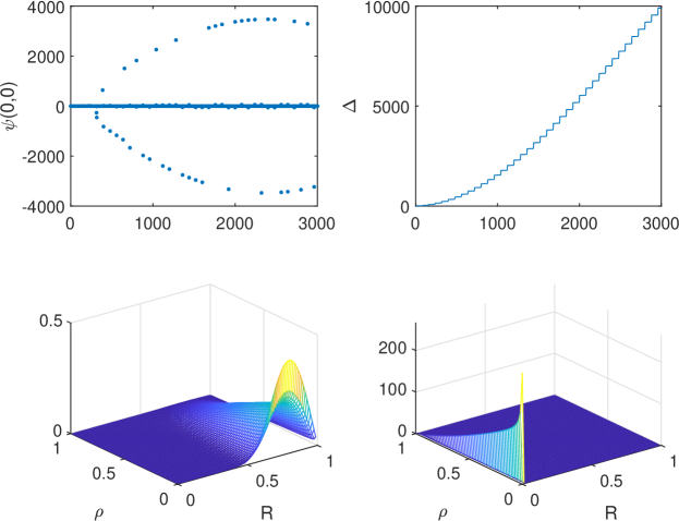
Figure 1: $\psi\left(0,0\right)$, the energy difference $\Delta$ between the ground and the excited states and the wave functions of the ground state and the first quantum triple collision state

The right upper panel shows the energy difference $\Delta$ between the ground state $\psi_{0}$ and the excited states (in $H$ units) and the two lower panels show respectively the wave functions of the ground state $\psi_{0}$ and of the first quantum triple collision state $\psi_{1}^{\ast}$.

The objective now is to assess the possibility of carrying the system from the ground state $\psi_{0}$ to the state $\psi_{1}^{\ast}$. The most effective way for coherently controlling the evolution of a quantum system is through the interaction between the system and an electromagnetic field whose spectral content and temporal profile may be altered throughout the process. The evolution equation would be

$$i\hslash\partial_{t}\psi\left(t\right)=\left(H-\epsilon\left(t\right)H_{1}\right)\psi\left(t\right)$$ (9)

where $H$ is the original Hamiltonian, $H_{1}$ the control operator and $\epsilon\left(t\right)$ the time varying control intensity. A well established technique of optimal control [10] [11] [12] defines a function $F$ , to be minimized, which contains both the objective goal and all the desired control constraints, among them the equation of motion (9). The constraints are made independent by the introduction of Lagrangian multiplier fields and the optimal control intensity $\epsilon\left(t\right)$ is obtained by iterative forward integration of (9) and backward integration of the Lagrange multiplier equations. This method allows the introduction of arbitrary control constraints, in particular the fluency $\int\epsilon\left(t\right)^{2}dt$ of the control field. An alternative local field approach, which will be used here, defines a Lyapunov function [13]

$$M\left(t\right)=\left(\psi\left(t\right),\psi_{1}^{\ast}\right)\left(\psi_{1}^{\ast},\psi\left(t\right)\right)$$ (10)

and chooses $\epsilon\left(t\right)$ during the evolution, with initial condition $\psi_{0}$, to insure that $\frac{d}{dt}M\geq 0$. Because

$$\frac{dM\left(t\right)}{dt}=-\epsilon\left(t\right)\frac{2}{\hslash}\mathnormal{Im}\left\{\left(\psi\left(t\right),\psi_{1}^{\ast}\right)\left(\psi_{1}^{\ast},H_{1}\psi\left(t\right)\right)\right\}$$ (11)

the condition $\frac{d}{dt}M\geq 0$ is satisfied if

$$\epsilon\left(t\right)=-\alpha\mathnormal{Im}\left\{\left(\psi\left(t\right),\psi_{1}^{\ast}\right)\left(\psi_{1}^{\ast},H_{1}\psi\left(t\right)\right)\right\}$$ (12)

$\alpha$ a positive constant.

Even for a system contained in a box, the Hilbert space of solutions of the equation (9) is infinite-dimensional and it is known that full quantum controllability in infinite dimensions is a delicate problem [14] requiring non-Lie algebraic operators or approximations thereof [15] [16]. In this case however one deals with a simpler problem of controllability between two states in a discrete spectrum. It is known that in this case a necessary condition [17] is transitivity of the operator $H_{1}$. Hence the first thing to check is the availability of $H_{1}$ operators that are transitive between these two states, in the sense that there is an iteration $H_{1}^{n}$ of the operator with non-vanishing matrix elements between the two states.

In the dipole approximation the interaction of the charged particles with the electric field of a laser pulse takes place through the dipole operator, namely

$$D=\left(R-\rho\right)\cdot E$$ (13)

with $Z=q=1$, $E$ the electrical field and all constants included in $\epsilon\left(t\right)$. To obtain the effect of this operator on the maximally symmetric states one integrates over all angles obtaining

$$H_{1}^{(E)}=\frac{1}{16R\rho}\left\{\left(R+\rho\right)^{3}-\left|R-\rho\right|^{3}\right\}$$ (14)

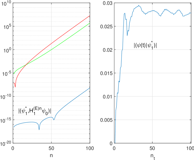
Figure 2: $\left|\left(\psi_{1}^{\ast},H_{1}^{(E)^{n}}\psi_{0}\right)\right|$ compared with similar matrix elements replacing $\psi_{1}^{\ast}$ by two states with $\psi(0,0)=0$ and a control attempt with the dipole operator. $n-_{t}$ is the number of control steps with $dt=0.05$

The transitivity of this operator is found by computing $\left|\left(\psi_{1}^{\ast},H_{1}^{(E)^{n}}\psi_{0}\right)\right|$ for successive powers of the operator. The result is shown in the left-hand panel of Fig.2 where this value is compared with the corresponding matrix element with $\psi_{1}^{\ast}$ replaced by two other randomly chosen states for which $\psi\left(0,0\right)=0$. This shows that, starting from the ground state, the quantum triple collision state is not controllable with this operator. This is confirmed in the right-hand panel where a control attempt is made using the Lyapunov method and adjusting the field $\epsilon\left(t\right)$ intensity at each step by (12). The time step is $dt=0.05$ and the exponential of the operator is computed at every step to improve the precision. One sees that the overlap $\left|\left(\psi_{0},\psi_{1}^{\ast}\right)\right|$ always remains at the level of the numerical round-off. The uncontrollability by the dipole operator is in fact to be expected because in the quantum triple collision state $R$ and $\rho$ are expected to be small, even for states that are not maximally symmetric. In the maximally symmetric case, studied here, one sees from Fig.1 that in the $\psi_{1}^{\ast}$ state $R\approx 0$ and therefore the operator $H_{1}^{(E)}$ in (14) vanishes.

For a controlling alternative one considers the interaction with a magnetic field $B$. This interaction has two different terms, the paramagnetic and the diamagnetic, both arising from the substitution $p\rightarrow p-eA\left(x,t\right)$ . The paramagnetic term may be written

$$-\frac{e}{2m}L\cdot B$$

and therefore, being proportional to the orbital angular momentum $L$, it vanishes for a maximally symmetric state. The diamagnetic term is proportional to

$$\rho^{2}\left(B_{z}^{2}+B_{y}^{2}\right)+Z\mu R^{2}$$

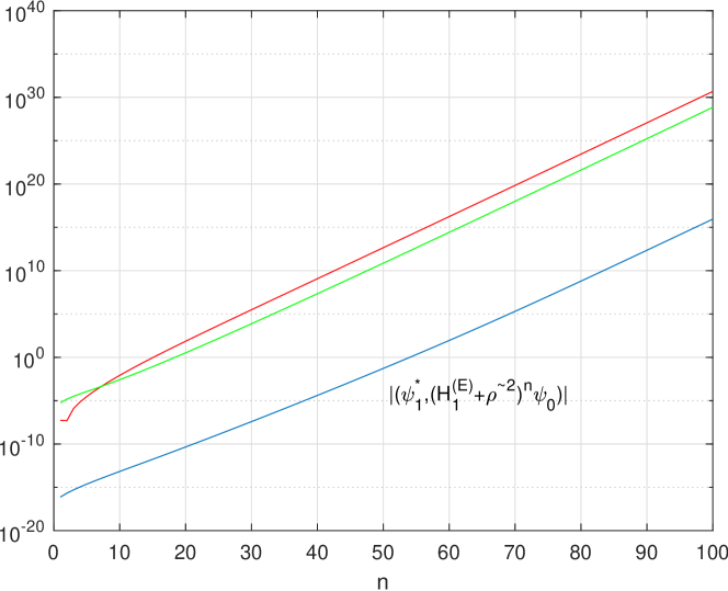
Figure 3: $\left|\left(\psi_{1}^{\ast},\left(H_{1}^{(E)}+\rho^{2}\right)^{n}\psi_{0}\right)\right|$ compared with similar matrix elements replacing $\psi_{1}^{\ast}$ by two states with $\psi(0,0)=0$

If $M\gg m$, $\mu$ is very small and will be mostly the operator $\rho^{2}\$ that might have a controlling effect. In Fig.3 one shows the successive values of $\left|\left(\psi_{1}^{\ast},\left(H_{1}^{(E)}+\rho^{2}\right)^{n}\psi_{0}\right)\right|$. Ones sees that in this case the matrix element becomes large, although not so large as the corresponding matrix elements for the same two reference states as used in Fig.2 . Some degree of controllability is confirmed by using again the Lyapunov method now with the operator

$$H_{1}^{(M)}=H_{1}^{(E)}+\rho^{2}$$

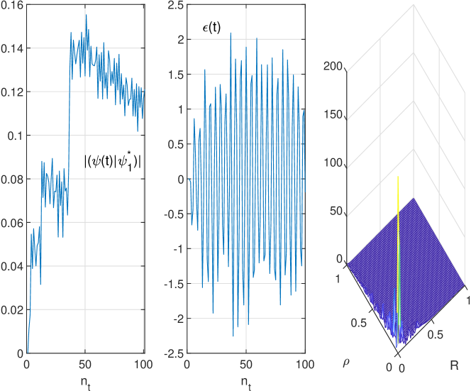
Figure 4: Control with the $H_{1}^{(M)}$ operator. The overlap $\left|\left(\psi\left(t\right),\psi_{1}^{\ast}\right)\right|$, the control intensity $\epsilon\left(t\right)$ and the wave function $\psi\left(t\right)$ after $100$ iterations

The result of the numerical calculation is shown in Fig.4 where one sees that the overlap indeed grows rapidly on the first four iterations then settling around $12\%$. The left-hand panel shows the overlap $\left|\left(\psi\left(t\right),\psi_{1}^{\ast}\right)\right|$, the middle one the control intensity $\epsilon\left(t\right)$ and the right-hand panel the wave function $\psi\left(t\right)$ after $100$ iterations. Although the controlled wave function is very close to a quantum triple collision situation, the overlap is still small because, as seen in right-hand panel, the coincidence with the objective function is mostly in the region of small $\rho$ and $R$ where the integration measure (7) is small.

In conclusion: A Coulomb system of two positive and one negative charge confined in a box has quantum triple collision states. These states are high excited states in the spectrum. They are many but still exceptional in a ”sea” of states with $\psi\left(0,0\right)=0$. Quantum control from the ground state, by the dipole operator, is not possible in maximally symmetric states and also expected to be inefficient for non-symmetric states. However, it seems possible using time-varying magnetic fields. Magnetic control might even be more efficient for non-symmetric states because of the action of the paramagnetic term.

Notice however that the non-controllability result with the dipole operator and the electric field refers only to exact controllability, which arises from the non-transitivity of the $H_{1}^{(E)}$ operator. What one observes, for example in the control experiment reported in the right-hand panel of Fig.2, is that the controlled wave function $\psi\left(t\right)$ converges to states of close proximity ($R$ small), nevertheless with negligible overlap with the objective function $\psi_{1}^{\ast}$.

In an actual 3-body Coulomb system confined in a solid lattice, accurate calculation of the energy levels will be difficult, because it is strongly influenced by the solid state environment. Therefore to have success in the use of quantum triple collisions to induce molecular or nuclear reactions, some experimental automatic learning process as in [18] is recommended.

References

- [1] C. Brif, R. Chakrabarti and H. Rabitz; Control of quantum phenomena: past, present and future, New Journal of Physics 12 (2010) 075008.
- [2] D. D’Alessandro; Introduction to quantum control and dynamics (2nd edition), CRC Press, Taylor and Francis, Boca Raton 2022.
- [3] C. P. Koch, M. Lemeshko and D. Sugny; Quantum control of molecular rotation, Rev. Mod. Phys. 91 (2019) 035005.
- [4] A. B. Magann, C. Arenz, M. D. Grace, T.-S. Ho, R. L. Kosut, J. R. McClean, H. A. Rabitz, and M. Sarovar; From pulses to circuits and back again: A quantum optimal control perspective on variational quantum algorithms, PRX Quantum 2 (2021) 010101.
- [5] P. Ballester, M. Fujita and J. Rebek (Ed.) , Molecular Containers, a special issue of Chem. Soc. Rev. 44 (2015).
- [6] E. J. Heller; Bound-state eigenfunctions of classically chaotic Hamiltonian systems: Scars of periodic orbits, Phys. Rev. Lett. 53 (1984) 1515-1518.
- [7] M. V. Berry; Quantum scars of classical closed orbits in phase space, Proc. R. Soc. London A 423 (1989) 219-231.
- [8] R. Vilela Mendes; Saddle scars: existence and applications, Phys. Lett. A 239 (1998) 223-227.
- [9] R. Vilela Mendes; On lattice confinement and hybrid fusion, Modern Physics Letters B 36 (2022) 2250042.
- [10] S. Shi and H. Rabitz; Optimal control of selectivity of unimolecular reactions via an excited electronic state with designed lasers, J. Chem. Phys. 97 (1992) 276-287.
- [11] D. J. Tannor and V. Kazakov; Control of photochemical branching: Novel procedures for finding optimal pulses and global upper bounds, in Time Dependent Quantum Molecular Dynamics, J. Broeckhove and L. Lathouwers (Eds.) pp. 347-360, Plenum Press, New York 1992.
- [12] Y. Maday and G. Turinici; New formulations of monotonically convergent quantum control algorithms, J. Chem. Phys. 118 (2003) 8191-8196.
- [13] M. Mirrahimi, P. Rouchon and G. Turinici; Lyapunov control of bilinear Schrödinger equations, Automatica 41 (2005) 1987-1994.
- [14] G. Turinici; On the controllability of bilinear quantum systems, in Mathematical models and methods for ab initio Quantum Chemistry, M. Defranceschi and C. Le Bris (Eds.) Lecture Notes in Chemistry vol. 74, pp. 75-92, Springer 2000.
- [15] W. Karwowski and R. Vilela Mendes; Quantum control in infinite dimensions, Physics Letters A 322 (2004) 282–285.
- [16] R. Vilela Mendes and V. I. Man’ko; On the problem of quantum control in infinite dimensions, J. Phys. A: Math. Theor. 44 (2011) 135302.
- [17] T. Chambrion, P. Mason, M. Sigalotti and U. Boscain; Controllability of the discrete-spectrum Schrödinger equation driven by an external field, Ann. I. H. Poincaré – AN 26 (2009) 329–349.
- [18] R. S. Judson and H. Rabitz; Teaching lasers to control molecules, Phys. Rev. Lett. 68 (1992) 1500.