Three-dimensional simulation of a core-collapse supernova for a binary star progenitor of SN 1987A

Abstract

We present results from a self-consistent, non-rotating core-collapse supernova simulation in three spatial dimensions using a binary evolution progenitor model of SN 1987A by Urushibata et al. (2018). This $18.3M_{\odot}$ progenitor model is evolved from a slow-merger of 14 and $9M_{\odot}$ stars, and it satisfies most of the observational constraints such as red-to-blue evolution, lifetime, total mass and position in the Hertzsprung-Russell diagram at collapse, and chemical anomalies. Our simulation is initiated from a spherically symmetric collapse and mapped to the three-dimensional coordinates at 10 ms after bounce to follow the non-spherical hydrodynamics evolution. We obtain the neutrino-driven shock revival for this progenitor at $\sim$ 350 ms after bounce, leading to the formation of a newly-born neutron star with average gravitational mass $\sim 1.35\,M_{\odot}$ and spin period $\sim 0.1$ s. We also discuss the detectability of gravitational wave and neutrino signals for a Galactic event with the same characteristics as SN 1987A. At our final simulation time ($\sim 660$ ms postbounce), the diagnostic explosion energy, though still growing, is smaller (0.15 foe) compared to the observed value (1.5 foe). The ⁵⁶Ni mass obtained from the simulation ($0.01M_{\odot}$) is also smaller than the reported mass from SN 1987A ($0.07M_{\odot}$). Long-term simulation including several missing physical ingredients in our three-dimensional models such as rotation, magnetic fields, or more elaborate neutrino opacities should be done to bridge the gap between the theoretical predictions and the observed values.

1 Introduction

SN 1987A, which emerged in the Large Magellanic Cloud located at a distance of $49.59\pm 0.63$ kpc (Pietrzyński et al., 2019), is a landmark event in astrophysics. Multiwavelength studies of SN 1987A have provided unprecedented details of supernova features such as the time evolution of the bolometric luminosity (Shigeyama et al., 1988; Shigeyama & Nomoto, 1990; Suntzeff & Bouchet, 1990) and energy spectrum at all wave bands from infrared to $\gamma$-ray (for a review of the observational features of SN 1987A, see, e.g., Arnett et al., 1989; McCray, 1993; McCray & Fransson, 2016). Moreover, a supernova neutrino burst was detected by several neutrino detectors such as Kamiokande-II (Hirata et al., 1987; Hirata et al., 1988), IMB (Bionta et al., 1987; Bratton et al., 1988), and Baksan (Alekseev et al., 1987; Alexeyev et al., 1988). Although only about two dozen of the $\sim 10^{28}$ supernova neutrinos that passed through the Earth were detected, they provided us with the first (and ever only one) direct evidence of the supernova (SN) driven by the collapsing core of a dying star (Sato & Suzuki, 1987). This detection implied that there had been a proto-neutron star at least for 10 seconds and it declared the dawn of the neutrino astrophysics.

The nature of the central remnant of SN 1987A – the compact remnant left behind the explosion is whether a neutron star or a black hole, for example – has been a mystery since observational searches for the remnant in radio and X-rays have been unsuccessful (e.g., Alp et al., 2018; Esposito et al., 2018) owing to the dust and the ring surrounding the supernova remnant. Recently, however, Cigan et al. (2019) have presented high angular resolution images of dust and molecules in SN 1987A ejecta obtained from the Atacama Large Millimeter/submillimeter Array (ALMA) and concluded that the presence of a compact source in the remnant is strongly indicated. The infrared excess could be due to the decay of isotopes like ⁴⁴Ti, accretion luminosity from a neutron star or black hole, magnetospheric emission, a wind originating from the spindown of a pulsar, or thermal emission from an embedded, cooling neutron star. Page et al. (2020) carefully investigated all possibilities and concluded that the cooling NS scenario is the most plausible.

The light curve and spectra indicate that SN 1987A has roughly typical explosion energy ($\sim 1.5\times 10^{51}$ erg, Jerkstrand et al., 2020) and ⁵⁶Ni mass ($0.07\,M_{\odot}$, Bouchet et al., 1991; McCray, 1993; Seitenzahl et al., 2014). On the other hand, SN 1987A is a unique supernova in many senses. First, a blue hot surface of the progenitor star Sk-69^∘202 found in the pre-explosion images (Blanco et al., 1987; Walborn et al., 1987), as well as the light curve without the typical plateau phase of type II-P SNe (Catchpole et al., 1988; Hamuy et al., 1988) and the relatively short period of time delay (three hours) between the neutrino burst detection and the shock breakout emission, suggest that the progenitor was a blue-supergiant (BSG) (Woosley et al., 1988; Arnett et al., 1989). Second, this BSG star is expected to have been a red-supergiant (RSG) $2\times 10^{4}$ yrs before exploding, since there are three ring-like nebulae surrounding the supernova remnant (Wampler & Richichi, 1989; Wampler et al., 1990; Burrows et al., 1995; France et al., 2010) with the high He and CNO abundance rations (Lundqvist & Fransson, 1996; Mattila et al., 2010) and the expansion velocity comparable to the RSG wind velocity.

To explain these anomalous features, many pre-explosion evolution scenarios of the progenitor star have been proposed soon after the emergence of SN 1987A (see Podsiadlowski 1992 for a review of the following classical progenitor models): extreme-mass-loss models (Maeder, 1987; Wood & Faulkner, 1987), helium-enrichment models (Saio et al., 1988), low-metallicity models (Arnett, 1987; Hillebrandt et al., 1987), rapid-rotation models (Weiss et al., 1988; Langer, 1991), and restricted-convection models (Woosley et al., 1988; Langer et al., 1989; Weiss, 1989). Also, binary interaction has been considered from early on: accretion models (Barkat & Wheeler, 1989; Podsiadlowski & Joss, 1989; De Loore & Vanbeveren, 1992), companion models (Fabian et al., 1987; Joss et al., 1988), and merger models (Hillebrandt & Meyer, 1989; Podsiadlowski et al., 1990).

The majority of massive stars live in binary or multiple systems (Duchêne & Kraus, 2013; Sana et al., 2013), and binary interactions can alter both the surface and core structure of the core-collapse supernova (CCSN) progenitor stars (Laplace et al., 2021; Vartanyan et al., 2021). One of the possible scenarios to the SN 1987A progenitor is a slow merger of binary stars where the stars in a close binary evolve into a common envelope phase after which the secondary star is gradually dissolved inside the common envelope in a much longer time-scale than the dynamical time-scale of the secondary (Podsiadlowski et al., 1990, 1992; Ivanova et al., 2002). Recently new progenitor models based on the slow merger scenario have been constructed (Menon & Heger, 2017; Urushibata et al., 2018). The models of Menon & Heger (2017) were the first to evolve a binary-merger model until core-collapse for SN 1987A’s progenitor and successfully reproduced the progenitor characteristics such as red-to-blue evolution, position in the Hertzsprung-Russell diagram at collapse, and the enrichment of helium and nitrogen in the progenitor, along with the lifetime of the BSG phase. Menon & Heger (2017) employed a simplified effective-merger model, and they did not compute mass loss in the merger phase. In contrast, Urushibata et al. (2018) have taken into account the spinning-up of the stellar envelope and subsequent mass loss due to angular momentum transportation from the orbit. They obtained enough mass ejection to explain the circumstellar nebula, as well as the characteristics of SN 1987A’s progenitor.

In parallel to the study of the progenitors of SN 1987A, a separate effort has been devoted to understand the explosion characteristics of SN 1987A, including the explosion energy, distribution of synthesized elements, emission of multimessenger signals and properties of the central remnant. Kifonidis et al. (2006) investigated matter mixing with realistic explosion models based on two-dimensional (2D) hydrodynamical simulations of neutrino-driven CCSNe aided by convection and/or SASI. The authors found that a globally aspherical explosion dominated by low-order unstable modes with explosion energy of $2\times 10^{51}$ erg produces high-velocity ⁵⁶Ni clumps as inferred from the observed [Fe II] line profiles in the remnant of SN 1987A. Wongwathanarat et al. (2015) investigated the dependence of matter mixing on single-star progenitor models based on three-dimensional (3D) hydrodynamic simulations and also obtained such a high-velocity ⁵⁶Ni. Utrobin et al. (2015) modelled optical light curves based on 3D hydrodynamic models. Among the investigated models, only one BSG model reproduces the dome-like shape of the light-curve maximum of SN 1987A. Utrobin et al. (2019) investigated matter mixing in explosions of a large sample of BSG models and concluded that single-star progenitor models have difficulties in reproducing observational constraints.

The binary-merger models of Menon & Heger (2017) were investigated by 1D explosion simulations (Menon et al., 2019). In comparison with the available single-star BSG progenitor models, the post-merger models were able to better reproduce the shape of the light curve of SN 1987A along with the light curves of other peculiar Type II supernovae like SN 1987A. Utrobin et al. (2021) performed 3D neutrino-driven explosions and followed the evolution of the shock wave long after explosion. They succeeded in reproducing the ⁵⁶Ni mass and mixing in the ejecta material, leading to a good reproduction of light curve of SN 1987A. Employing the binary progenitor model of Urushibata et al. (2018) and FLASH code (Fryer & Heger, 2000), Ono et al. (2020) performed hydrodynamic simulations in the 3D Cartesian coordinates focusing on the matter mixing in SN 1987A. They succeeded in reproducing high-velocity ⁵⁶Ni inferred from the observed [Fe II] line profiles in the remnant of SN 1987A. In all of these simulations based on single-star and binary progenitor models, the inner region corresponding to a compact object was excluded from the calculation and a parametric energy or neutrino emission was injected to drive an explosion.

In this paper, we report the results of our self-consistent 3D CCSN simulation employing the binary-merger progenitor model of Urushibata et al. (2018). We solve hydrodynamic evolution and energy-dependent neutrino transport from the centre to the outer boundary at 10,000 km. A number of self-consistent 3D simulations with energy-dependent neutrino transport (e.g. Takiwaki et al., 2014; Melson et al., 2015a; Melson et al., 2015b; Lentz et al., 2015; Janka et al., 2016; Ott et al., 2018; Summa et al., 2018; Müller et al., 2018; Müller et al., 2019; Burrows et al., 2020; Iwakami et al., 2020; Stockinger et al., 2020; Takiwaki et al., 2021; Matsumoto et al., 2022) have recently been demonstrated based on the neutrino-driven mechanism (Colgate & White, 1966; Arnett, 1966; Bethe & Wilson, 1985). Our simulations have an advantage in taking account of nuclear network calculation so that we can provide an estimate of explosive nucleosynthesis yield. Furthermore, we investigate in detail the properties of the SN 1987A’s central remnant and multi-messenger signals obtained from the results of the 3D self-consistent simulation.

This paper is organized as follows. Section 2 summarizes our numerical methods and the progenitor model employed in this work. We present our 3D results in section 3, which consists of shock evolution (§3.1), neutrino emission and PNS convection (§3.2), and multimessenger signals including gravitational wave (§3.3). We conclude with discussions in section 4.

2 Numerical setups

The progenitor model we use is based on the slow merger scenario (Podsiadlowski et al., 1990, 1992), which explains the evolution of SN 1987A progenitor from an RSG to a BSG as a result of stellar merger and deflation of the primary RSG in a binary system. Recently, similar attempts to model the evolution of the SN 1987A progenitor star, Sk -69^∘202, have been presented (Menon & Heger, 2017; Urushibata et al., 2018). In particular, Urushibata et al. (2018) have considered the spinning-up of the stellar envelope and their best model ($14+9M_{\odot}$ binary with a particular parameter set of merging) successfully reproduced the progenitor characteristics such as the N/C ratio of the stellar surface and the timing of the blueward evolution of $2\times 10^{4}$ yr before the collapse, as well as the mass ejection into the circumstellar medium. Therefore, we employ the $14+9M_{\odot}$ progenitor model (hereafter m14 model) from Urushibata et al. (2018). This progenitor is studied by Ono et al. (2020) focusing on a matter mixing in the outer envelope using FLASH code, and we employ the radiation/hydrodynamic code 3DnSNe (Takiwaki et al., 2016; Takiwaki & Kotake, 2018) to study the dynamical evolution of the core of this progenitor model as a central engine of SN 1987A.

Figure 1 describes the structure of the m14 model, compared with 16 and $20M_{\odot}$ pre-SN RSG models from Woosley & Heger (2007). There is an outstanding difference in the density profile (left panel) in the outer envelope since the BSG SN 1987A progenitor has a much smaller radius than the other RSG progenitors. Note that our simulations are within $10^{9}$ cm from the center. Given that the progenitor’s compactness parameter $\xi_{M}$, which is defined in O’Connor & Ott (2011) as a function of an enclosed mass $M$,

$$\xi_{M}=\frac{M\,[M_{\odot}]}{R(M)\,[1000\,{\rm km}]},$$ (1)

is a good diagnostics for the explosion properties. The right panel of Figure 1 shows the compactness $\xi_{M}$ as a function of the enclosed mass. The m14 model lies between s16 and s20 models, both of which are reported to explode in 3D simulations in a self-consistent manner (Vartanyan et al., 2019; Melson et al., 2015b) via neutrino heating, namely without additional input of energy nor increase in the heating rate.

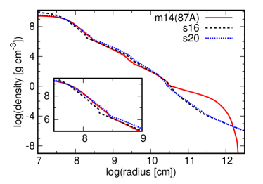
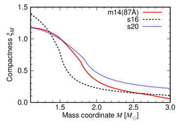
Figure 1: The structure of the SN 1987A progenitor model (m14, Urushibata et al., 2018) compared with 16 and $20M_{\odot}$ pre-SN models from Woosley & Heger (2007). Left panel: Density profiles of the progenitors. The SN 1987A progenitor is a BSG star and its radius is about one order of magnitude smaller than RSG stars with an extended hydrogen envelope. In the inset, we show the zoomed-in density profile around the iron core surface located at $r\sim 10^{8.3}$ – $10^{8.5}$ cm. Right panel: the compactness parameter of these three progenitor models as a function of enclosed mass. The compactness of the SN 1987A progenitor is smaller than that of s20 model, which has been reported to explode in 3D simulation (Melson et al., 2015b).

The 3DnSNe code that we employ in this study is a multi-dimensional, three-neutrino-flavour radiation hydrodynamics code constructed to study core-collapse supernovae. The neutrino transport is solved by the isotropic diffusion source approximation (IDSA) scheme for electron, anti-electron, and heavy lepton neutrinos (Liebendörfer et al., 2009; Takiwaki et al., 2016) taking the state-of-the-art neutrino opacity (Kotake et al., 2018) and discretized neutrino spectrum with 20 energy bins for $0<\epsilon_{\nu}\leq 300$ MeV. Takiwaki & Kotake (2018) have implemented the gravity potential taking account of the effective General Relativistic effect (case A in Marek et al., 2006).

The spatial range of the 1D, 2D, and 3D computational domain is within $r<$10,000 km in radius and divided into 600 non-uniform radial zones. Our spatial grid has the finest mesh spacing $dr_{\rm min}=250$ m at the centre, and $dr/r$ is better than 1.0 % at $r>100$ km. The 2D model is computed on a spherical coordinate grid with an angular resolution of $n_{\theta}=128$ zones. For 3D model we simulate with the resolution of $n_{\theta}\times n_{\phi}=64\times 128$ zones. Seed perturbations for aspherical instabilities are imposed by hand at 10 ms after bounce by introducing random perturbations of $0.1\%$ in density on the whole computational grid except for the unshocked core. Regarding the equation of state (EOS), we use that of Lattimer & Swesty (1991) with a nuclear incomprehensibility of $K=220$ MeV. At low densities, we employ an EOS accounting for photons, electrons, positrons, and ideal gas contribution. We follow the explosive nucleosynthesis by solving a simple nuclear network consisting of 13 alpha-nuclei, ⁴He, ¹²C, ¹⁶O, ²⁰Ne, ²⁴Mg, ²⁸Si, ³²S, ³⁶Ar, ⁴⁰Ca, ⁴⁴Ti, ⁴⁸Cr, ⁵²Fe, and ⁵⁶Ni. A feedback from the composition change to the EOS is neglected, whereas the energy feedback from the nuclear reactions to the hydrodynamic evolution is taken into account as in Nakamura et al. (2014).

Along with these setups, we simulate core collapse, bounce, and subsequent shock evolution under the influence of neutrino heating. Our simulations are self-consistent in the sense that we do not employ any artificial control to drive explosions. Note that there is a consensus that a successful supernova explosion driven by neutrino heating cannot be achieved under the spherical symmetry (1D) (Liebendörfer et al., 2001; Sumiyoshi et al., 2005), except for a few less massive stellar models (e.g., Kitaura et al. (2006) for an O-Ne-Mg core and Mori et al. (2021); Nakazato et al. (2021) for an iron core). Note also that we simulate the core collapse and bounce in 1D geometry and then map it to the 3D coordinates at 10 ms after bounce to follow non-spherical evolution, whereas 2D simulation is initiated from the beginning of the collapse. This difference in the numerical treatment until the core bounce does not play any significant role since our simulations start from the spherically symmetric progenitor and non-spherical motions are developed only after the bounce by hydrodynamic instabilities.

3 Results

This section reports the results of our core-collapse simulations for the latest SN 1987A progenitor model, primarily focusing on the 3D simulation. Our simulations are based on the neutrino heating mechanism and failed in explosion for the 1D spherically symmetric case, whereas succeeded in shock revival for 2D and 3D models. First we summarize shock evolution driven by neutrino heating (3.1), then examine neutrino properties as well as PNS convection which affects neutrino emission (3.2). We also estimate some observable values adopting the current and future neutrino and gravitational wave (GW) detectors (3.3).

3.1 Shock evolution

Figures 2 and 3 show early evolution of shock radius and some relevant values representing the condition of neutrino-heated matter behind the shock. The shock of our 3D model once stalls at $r\sim 150$ km, gradually shrinks down to $\sim 120$ km, then turns to expand at $\sim 220$ ms after bounce (top panel of Figure 2). The corresponding 1D simulation does not explode, whereas it is not shown in Figure 2. To assess the mechanism of the shock revival we estimate and compare two timescales, the advection time, $\tau_{\rm adv}=\int\frac{dr}{|v_{r}|}$, and the heating time, $\tau_{\rm heat}=\frac{\int e_{\rm bind}dV}{\int\dot{q}dV}$, where $v_{r}$ is the angle-averaged radial velocity, $e_{\rm bind}$ is the binding energy of the matter, $\dot{q}$ is the local heating rate by neutrino, and all of them are integrated over the gain region. Here the gain region is the region where the neutrino heating overcomes neutrino cooling, located behind the shock and extended to typically 50–60 km from the centre. The ratio of the advection to heating timescales are shown in the bottom panel of Figure 2. Preceding to the shock revival, the time ratio clearly exceeds one at $\sim 200$ ms after bounce, which means that the matter behind the shock could become unbound by neutrino heating before it passes through the gain region.

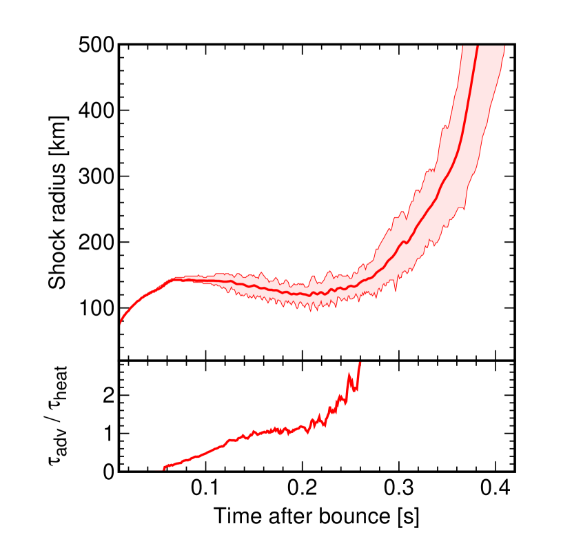
Figure 2: Top panel: The early time evolution of the shock radius for the 3D model. The coloured-in region indicates the range of the shock location from minimum to maximum. The shock once stalls at $r\sim 150$ km, gradually retreats, then turns to expand at 220 ms after bounce. Shown in the bottom panel is a ratio of advection timescale to neutrino heating timescale. The timescale ratio clearly exceeds unity just prior to the shock revival, which suggests that the shock revival is driven by neutrino heating.

To visualize the motion of matter caused by neutrino heating, we present anisotropic velocity profile in Figure 3. Here we define the anisotropic velocity, $v_{\rm aniso}$, following Takiwaki et al. (2012) as

$$v_{\rm aniso}=\sqrt{\langle\rho\left((v_{r}-\langle v_{r}\rangle)^{2}+v_{\theta}^{2}+v_{\phi}^{2}\right)\rangle/\langle\rho\rangle},$$ (2)

where the symbol $\langle x\rangle$ denotes angle average of $x$. We see that anisotropic motion in the gain region appears around $r\sim 80$ km at $\sim 150$ ms after bounce. The turbulent motion develops and extends to the shock front at $\sim 220$ ms after bounce, then the shock expansion accelerates and never retreats.

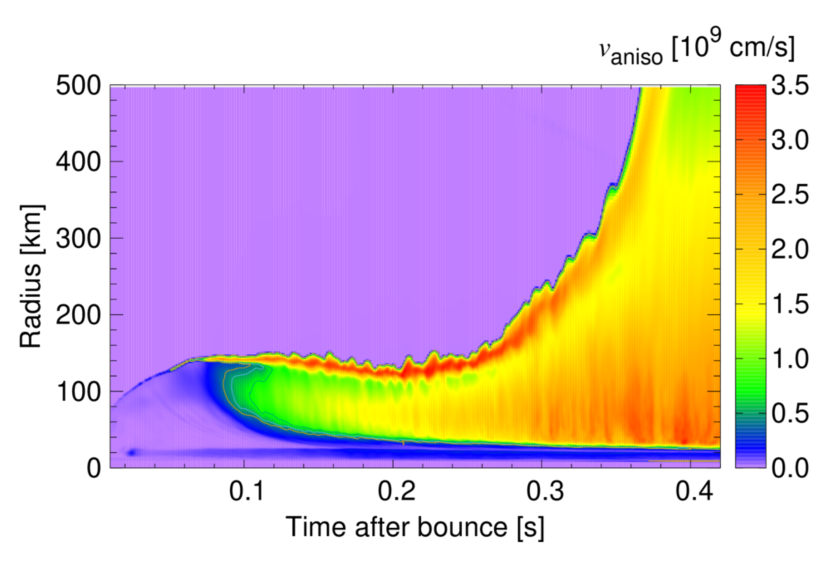
Figure 3: A space-time diagram of the anisotropic velocity. The yellowish region with high anisotropic velocity appears in the gain region at $t_{\rm pb}\sim 150$ ms, then the turbulent region spreads and pushes the stalled shock outward.

The 3D morphology of the shocked matter and the highly non-axisymmetric nature of the explosion are visualized in Figure 4. By $\sim 150$ ms after bounce, small-scale convective motion develops behind the shock and it slightly deforms the shock structure (left panel). The continuous neutrino heating and the convective motion finally make the stalled shock turn to expand. The expanding shock deviates from spherical symmetry, but it has no specific direction in our 3D model.

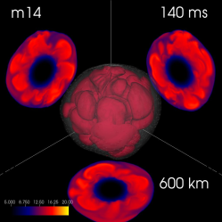
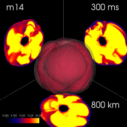
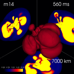
Figure 4: Time sequence of the isosurface of entropy, showing the morphology of the hot bubbles within the inner core of the exploding SN 1987A progenitor. Shown are three snapshots at 140 ms (left panel), 300 ms (middle), and 560 ms (right) after bounce. The time and spatial scales (box size) are noted in each panel. The contours on the cross-sections in the $x=0$, $y=0$, and $z=0$ planes are projected on the walls at the back right, back left, and bottom of each panel, respectively. Several high-entropy hot bubbles are visible, which push the shock outward without any dominant direction.

3.2 Neutrino emission and PNS convection

The behaviour of the matter behind the shock and the shock itself implies that neutrino heating plays a critical role in our 3D explosion model. Figure 5 shows luminosity and average energy of electron, anti-electron, and heavy lepton neutrinos ($\nu_{\rm e}$ , $\bar{\nu}_{\rm e}$, and $\nu_{\rm x}$) of our 3D model (thick red lines) compared with that of 1D model (thin gray lines) for reference. For the $\nu_{\rm e}$ and $\bar{\nu}_{\rm e}$ luminosity, both 1D and 3D models show sudden drop at $\sim 360$ ms after bounce (left panel). Prior to this luminosity drop, the Si/O interface falls onto the central region. The mass accretion rate decreases, resulting in a decrease in the release rate of gravitational energy carried by the accreting matter. The decrease of the accretion also causes a shock expansion in the 3D model, and the accretion rate drops further. In contrast, the 1D model does not present shock revival and keeps relatively high neutrino luminosity compared with the 3D model.

On the other hand, The $\nu_{\rm x}$ luminosity does not show such a sudden drop since $\nu_{\rm x}$ mainly comes from deep inside the core. Moreover, the $\nu_{\rm x}$ luminosity of the 3D model is higher than that of the 1D model. The deviation of the $\nu_{\rm x}$ luminosity between 1D and 3D models becomes visible at $\sim 150$ ms after bounce, which is roughly corresponding to the time when the anisotropic motion becomes outstanding in the 3D model (Figure 3). The turbulent motion seen in Figure 3, however, first appears at $r\sim 80$ km, which is out of neutrino spheres. It implies that this turbulent motion in the 3D model does not play a significant role in the deviation of neutrino properties from the 1D model.

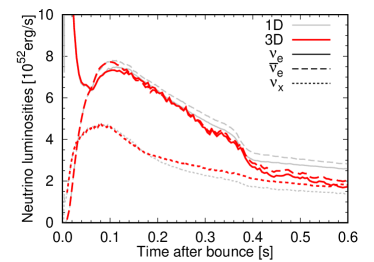
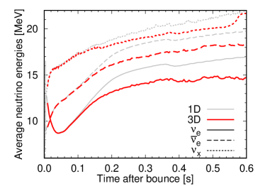
Figure 5: Neutrino luminosity (left panel) and average neutrino energy (right panel) as a function of time after bounce. The luminosities and average energies for the 3D model (thick red lines) are compared with those for the 1D model (thin grey lines), showing smaller values except $\nu_{\rm x}$ luminosity under the influence of the shock revival followed by a feeble accretion in the 3D model.

Again, since $\nu_{\rm x}$ mainly comes from deep inside the core, we provide a space-time diagram of the anisotropic velocity within the inner 100 km in Figure 6 to assess hydrodynamic motions deep inside the core. Two convective regions, the exterior neutrino-driven convection as in Figure 3 and the interior convective band around $r\sim 20$ km, are visible in this zoom-in panel. The interior convective zone first emerges at $\sim 25$ ms after bounce, then once becomes weaken and again active at $\sim 150$ ms. This may cause effective transport of diffusive neutrinos inside the PNS and explain the increase of $\nu_{\rm x}$ luminosity in the left panel of Figure 5 as discussed in Buras et al. (2006) and Nagakura et al. (2020). Furthermore, the interior convective motions hold up the PNS structure and the PNS radius of the 3D model becomes larger than that of the 1D model. This leads to a lift of neutrino sphere radius and a 1–2 MeV decrease of average neutrino energy of the 3D model compared to that of the 1D model as observed in the right panel of Figure 5 after $\sim 150$ ms and later.

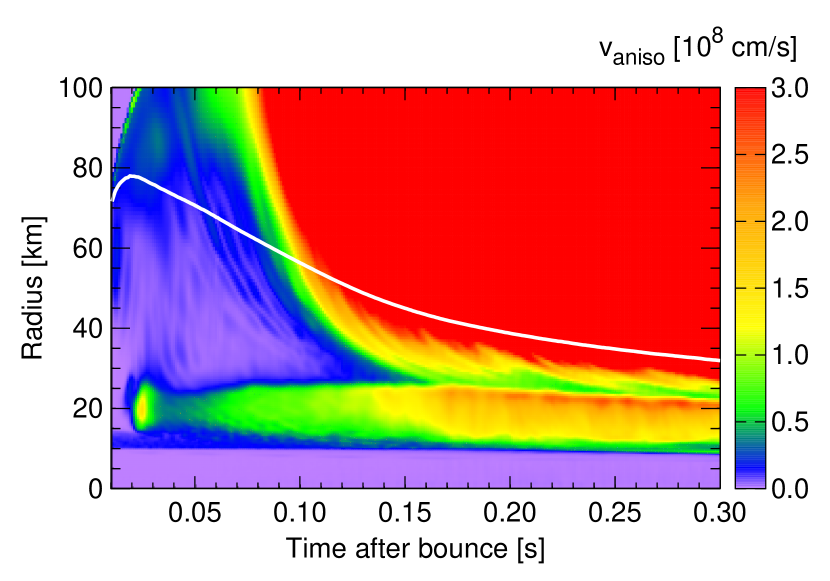
Figure 6: A space-time diagram of the anisotropic velocity for the 3D model as in Figure 3, but within the inner 100 km through 0.3 s after bounce. The inner PNS convective region is visible around $r\sim 20$ km. The white line illustrates the mean PNS radius defined as the radius where mass density $\rho=10^{11}\,{\rm g\,cm}^{-3}$.

Tamborra et al. (2014) found in their 3D CCSN model that the lepton-number flux ($\nu_{\rm e}$ minus $\bar{\nu}_{\rm e}$) emerges predominantly in one hemisphere, termed “Lepton-number Emission Self-sustained Asymmetry (LESA)”. We evaluate signatures of LESA in our 3D model. Following Glas et al. (2019), the moments of the lepton-number flux are evaluated as

$$A_{\rm lnf}(r,l)=\sqrt{\sum_{m=-l}^{l}[c_{l}^{m}(r)]^{2}},$$ (3)

where the multipole coefficients $c_{l}^{m}(r)$ at a given radius $r$ are calculated by integrating the flux over the whole spherical surface

$$c_{l}^{m}(r)=\sqrt{\frac{4\pi}{2l+1}}\int r^{2}F_{\rm lnf}^{\rm lab}Y_{l}^{m}d\Omega,$$ (4)

using the radial number flux of neutrino $F_{\rm lnf}^{\rm lab}$ in the lab frame. The time evolution of the multipole moments $A_{\rm lnf}$ of the electron lepton-number flux is shown in Figure 7. High order modes with $l=4$ and $l=5$ are excited first at $\sim 60$ ms after bounce. The emergence of these asymmetric neutrino fluxes roughly coincides with the time when the convective motion inside the PNS sets in (Figure 6). A dominant dipole ($l=1$) begins to appear at $\sim 170$ ms after bounce and the dipole and quadrupole ($l=2$) modes have dominant amplitudes until the end of our simulation. Such a time-evolving mode shift is consistent with Glas et al. (2019) who examine the effects of LESA with different progenitors, neutrino transport treatment, and grid resolutions.

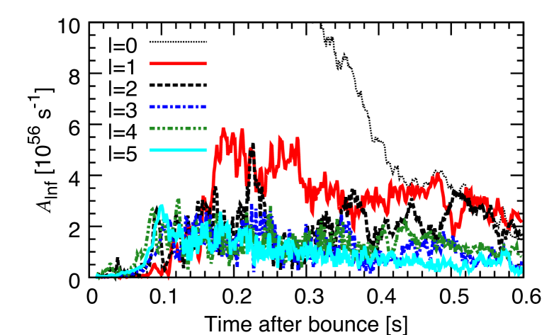
Figure 7: Monopole and multipole moments of the electron lepton-number flux for 3D models, evaluated at a radius of $r=500$ km and transformed into the lab frame at infinity, as functions of time after core bounce. The multipole amplitudes $A_{\rm lnf}$ are defined as given in Equation (3), while for $l=0$ the corresponding amplitude agrees with the total electron lepton-number flux.

3.3 Multi-messenger observables

At the end of our 3D simulation ($\sim 660$ ms after bounce), the average and the maximum shock radius have reached at $\sim 3000$ km and $\sim 4400$ km. The diagnostic explosion energy grows up to $E_{\rm diag}\sim 0.14\times 10^{51}$ erg by this time (Figure 8). Here the diagnostic explosion energy is defined as the sum of internal, kinetic, and gravitational energy in unbound materials with positive radial velocity. The electromagnetic lightcurve of SN 1987A is different from that of typical type IIP supernovae, but it can be reproduced by an explosion of a BSG with explosion energy $E_{\rm exp}\sim 1.5\times 10^{51}$ erg (Jerkstrand et al., 2020), one order of magnitude larger than the diagnostic explosion energy of our 3D model. The feeble explosion results in a small mass of ⁵⁶Ni yield. We obtain a rough estimate of ⁵⁶Ni mass, $M_{\rm Ni}$, in the unbound materials less than $0.01\,M_{\odot}$ by means of a simple 13 $\alpha$ network calculation, whereas the the value estimated from observations is $M_{\rm Ni}\sim 0.07\,M_{\odot}$ (Bouchet et al., 1991; McCray, 1993; Seitenzahl et al., 2014). Note that Sawada & Maeda (2019) and Sawada & Suwa (2021) argue that the timescale of the shock revival affects the ⁵⁶Ni yield. Their analysis indicates that the shock revival should occur earlier to obtain more yields.

The time evolution of the explosion energy and ⁵⁶Ni are compared to the results in 2D simulation in Figure 8. The 2D model assuming axi-symmetry presents a more energetic explosion with $E_{\rm diag}\sim 0.38\times 10^{51}$ erg and $M_{\rm Ni}\sim 0.04\,M_{\odot}$. The reason of the weak explosion in our 3D model will be discussed in §4.

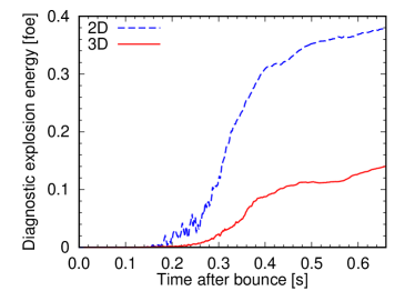
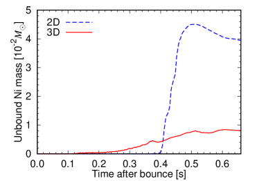
Figure 8: Time evolution of diagnostic explosion energy (left panel) and unbound Ni mass (right panel) of 2D and 3D models.

3.3.1 Neutrino

Our 3D model is not capable of direct comparison with SN 1987A observations. Below in this subsection, we assume that a supernova modelled by our 3D simulation occurs at the Galactic centre at the distance of 10 kpc and evaluate the multi-messenger signals like neutrino and gravitational wave from the CCSN. Figure 9 shows the neutrino detection event rate per 1 s bin expected by the Super-Kamiokande (SK) detector for the 10 kpc CCSN event. Here we only take account of inverse-beta events and do not consider MSW mixing (e.g., Kotake et al. (2006) for a review) and collective neutrino oscillations (see, e.g., Mirizzi et al., 2016; Horiuchi & Kneller, 2018; Shalgar & Tamborra, 2019, 2021; Abbar et al., 2019; Chakraborty & Chakraborty, 2020; Cherry et al., 2020; Sasaki et al., 2020; Sasaki & Takiwaki, 2021; Kato et al., 2020; Kato et al., 2021; Richers et al., 2021; Zaizen et al., 2021; Nagakura et al., 2021a; Harada & Nagakura, 2022; Sigl, 2022, for collective references therein). The high-statistics event curve will bring us plenty of information. The sudden drop at 0.35–0.4 s after bounce corresponds to the time of shock revival when the stalled shock turns to expand and neutrino luminosity from accreting matter decreases. Another revelation is a precise estimate of the bounce time, which is critical to reducing the background noise for gravitational wave detection (see Nakamura et al., 2016, for the discussion of multimessenger signals from a Galactic CCSN).

To obtain the whole neutrino light curve and spectrum from the supernova, we have to perform long term simulations, whose simulation time should be longer than $10\,{\rm s}$ (e.g., Suwa et al., 2019; Nakazato et al., 2022), which is beyond the scope of this paper. The relation between the character of PNS (e.g., mass and radius) and the neutrino luminosity is an important subject to investigate (Nakazato & Suzuki, 2019; Nagakura & Vartanyan, 2021). For this purpose an analytic solution of the light curve would be useful (Suwa et al., 2021).

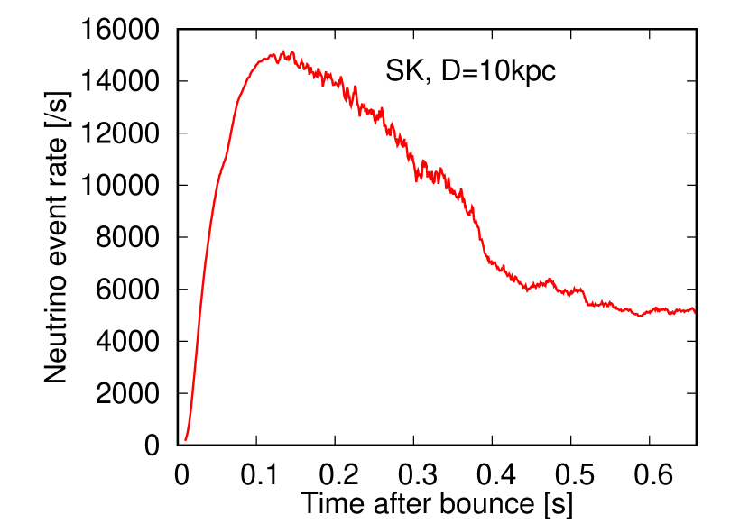
Figure 9: Expected neutrino events at Super-Kamiokande (SK) in 1 second time bins. Here we assume SK detector with an effective volume of 32 kton and the distance to the CCSN event of 10 kpc.

3.3.2 Gravitational wave

A gravitational-wave (GW) signal from CCSN is very weak compared to that from compact merger event. Once the neutrino detection event tells us the time of core bounce, however, a small time window for analysis is specified and background noise is greatly suppressed so that we expect gravitational wave detection from a Galactic core-collapse event (Nakamura et al., 2016). This detection is expected to revolutionize our CCSN theory (see, e.g., Kotake, 2013; Kuroda et al., 2016; Andresen et al., 2019; Radice et al., 2019; Abdikamalov et al., 2020; Müller & Varma, 2020; Mezzacappa et al., 2020; Eggenberger Andersen et al., 2021, for collective references therein) because the GW signals deliver the live information to us, which imprints the non-spherical hydrodynamics evolution up to the onset of explosion. Figures 10 and 11 show GW waveform of plus and cross modes ($h_{+}$ and $h_{\times}$, top windows) and a colour map of frequency $f$ components (spectrogram, bottom windows) as a function of time after bounce.

In Figure 10 we assume that an observer is along the $x$-axis of the simulation coordinates. One can see a typical time series of CCSN-GW characteristics both in plus and cross modes: first (0 to $\sim 50$ ms), a GW signal from prompt convection induced by a negative entropy gradient after the stalling shock appears in the wide range of frequency, followed by a relatively silent phase lasting from $\sim 50$ ms to $\sim 150$ ms, and then nonlinear fluid motions behind the shock excite strong high-frequency signals (starting from $f\sim 500$ Hz at 150 ms and growing up to $f>1000$ Hz at $\sim 400$ ms), which is attenuated as the shock expands and the nonlinear motions behind the shock are diluted ($t_{\rm pb}>400$ ms). Another component can be seen at around 100–300 Hz after $\sim 150$ ms. Kuroda et al. (2016) pointed out that the low frequency GW excess is correlated to the SASI in a similar frequency range . However, it should be noted that our model does not present SASI-like motion. This low-frequency signal in our model seems to correspond to a turn over timescale of the inner PNS convective motions (Figure 6) which emerges at $\sim 150$ ms in the radius around $10^{6}$ cm with 1–3 $\times 10^{8}\,{\rm cm\,s}^{-1}$ (see Mezzacappa et al. 2020 and discussion in Eggenberger Andersen et al. 2021, and also Nagakura et al. (2021b, c) for the neutrino signature).

In the left panels of Figures 10 and 11, showing the GW signal from the central ($<100$ km) matter, the amplitude is close to zero at the final phase. On the other hand, the amplitude of the total signal in the right panels deviates from zero. This is caused by the non-spherical motions of matter behind the shock.

A view from the polar ($z$-axis) direction (Figure 11) shows a similar time-evolution of GW waveform and spectrogram except for the prompt convection signal. We cannot unambiguously identify the reason of very weak prompt convection signal in the polar view. This may stem from a stochastic nature of prompt convection, the growth of which could happen to be direction-dependent.

We analyse a time-frequency behaviour of perturbative fluid motions by means of an open-source General Relativistic Eigen-mode Analysis Tool (GREAT, Torres-Forné et al., 2019) with changing the boundary condition (Sotani & Takiwaki, 2020a). We find some characteristic modes and overplot them on the GW spectrogram in the right panels of Figures 10 and 11. The most dominant frequency component appears at $\sim 150$ ms after bounce with $\sim 500$ Hz and evolves to more than 1000 Hz. This can be fitted by the $g1$ mode at first and shift to the $f$ mode at $\sim 250$ ms after bounce (Sotani et al., 2017; Morozova et al., 2018; Sotani & Takiwaki, 2020b). Relatively weak low-frequency (100–300 Hz) components after $\sim 150$ ms are fitted by the $g3$ and $g4$ modes.

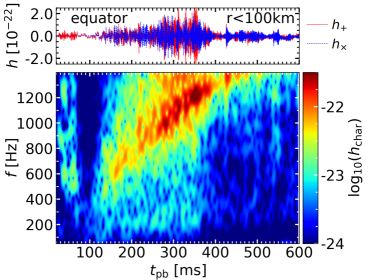
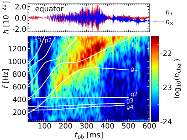
Figure 10: GW waveform and spectrogram of our 3D model viewed from the equator ($x$-axis) direction. Left panel: the input waveform in the top window and the Fourier-transformed spectrogram in the bottom window. GW source is limited within $r<100$ km. Right panel: same as the left panel but for the total GW signal. Overplotted are some characteristic gravitational wave frequencies calculated with GREAT.

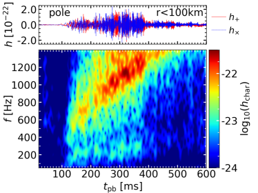
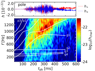
Figure 11: Same as Figure 10 but viewed from the polar ($z$-axis) direction.

Figure 12 presents GW spectra of our supernova model as a function of GW frequency $f$, compared with the detection sensitivity curves of some current and future GW detectors. Here we again assume the distance to the supernova to be 10 kpc. The detectors currently in operation (KAGRA, advanced LIGO, and advanced Virgo) have sensitivity to the GW signal for $f>100$ Hz with S/N ratio $>10$ and can be available for the analysis of the dominant high-frequency GW signals. The design sensitivity of Einstein Telescope and Cosmic Explorer is good enough for a wide range of frequencies covering $f<100$ Hz. Although such next-generation detectors or very nearby supernova events are desirable, the possible PNS convection signal ($\sim 200$ Hz) could be detectable by the current detectors.

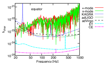
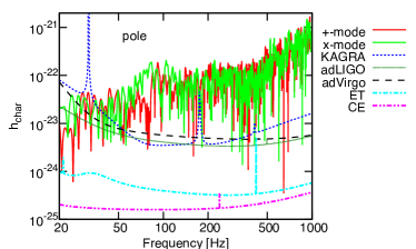
Figure 12: The gravitational wave spectra of our 3D model (solid lines) are compared with some detection sensitivity curves of current and future GW detectors. Shown are two cases that observers stand along the $x$-axis (left panel) and along the $z$-axis (right panel).

3.3.3 Neutron star kick and spin

A proper motion of the neutron star left behind the explosion is also meaningful. When a CCSN explosion is initiated in a non-spherical manner, the neutron star could be “kicked” by asymmetric hydrodynamic motions and mass ejection or by anisotropic neutrino emission from the PNS. Following the hydrodynamic kick scenario, we estimate the NS kick velocity as in Nakamura et al. (2019) (Figure 13). In this scenario, the kick velocity is determined by the net momentum of ejecta which is tightly connected to the explosion energy, asymmetricity of the ejecta motion, and the PNS mass. Nakamura et al. (2019) demonstrated long-term 2D CCSN simulations and concluded that the total momentum of the ejecta, or the explosion energy, is a predominant factor determining the strength of hydrodynamic kick, and the ejecta asymmetry plays a secondary role. Our 3D model has small explosion energy and roughly spherical mass distribution at least in the beginning of shock expansion, resulting in small kick velocity ($\sim 70\,{\rm km\,s}^{-1}$ at $t_{\rm pb}=660$ ms, red solid line in the right panel of Figure 13). Explosion models associated with jet-like structures have been studied to make the fast-moving heavy elements and the observed luminosity in SN 1987A (Nagataki, 2000) or to reproduce some morphological features of the remnant (Bear & Soker, 2018). Our axi-symmetric explosion of the 2D model does not hold a collimated jet, but it presents more energetic explosion and highly asymmetric mass distribution than the 3D model, leading to higher kick velocity ($>400\,{\rm km\,s}^{-1}$, dashed blue line).

Optical, X-ray, and gamma-ray light curves of SN 1987A and broad emission lines of heavy elements have strongly suggested large-scale mixing during the explosion (Kumagai et al., 1988, 1989; Hachisu et al., 1990). Morphology and the properties extracted from photometric and spectral observations of SN 1987A have revealed that the distribution of the matter ejected from SN 1987A is completely non-spherical (Wang et al., 2002; Larsson et al., 2013). Moreover, there is an intricate triple-ring structure around SN 1987A, reflecting non-spherical mass ejection in the evolution of the pre-SN. Observations of emission lines in the nebula phase have found a fast-moving iron clump and low-velocity hydrogen mixed down into the innermost ejecta, which can be reproduced by matter mixing via Rayleigh-Taylor instabilities at the chemical composition interfaces in the ejected envelope (Wongwathanarat et al., 2015; Utrobin et al., 2015, 2019; Utrobin et al., 2021; Ono et al., 2020), although it can not be captured by our space and time limited simulations. The NS kick is less affected by these asymmetries since they develop at locations far from the central core and the kick should be imposed in the early phase of the explosion.

Recently ALMA observation found an infrared excess source in the remnant of SN 1987A (Cigan et al., 2019; Page et al., 2020). Assuming that there is a cooling NS at the peak of the infrared excess, the NS kick velocity is estimated as $\sim 700\,{\rm km\,s}^{-1}$ from the deviation between the locations of the NS and the progenitor star (Cigan et al., 2019). Although this estimation involves large uncertainties, the high kick velocity implies that SN1987A was highly asymmetric in the very beginning of shock evolution.

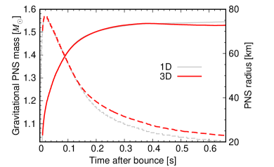
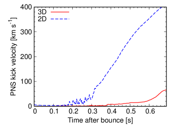
Figure 13: Left: The PNS mass (solid lines) and radius (dashed lines) for the 1D (thin grey) and 3D (thick red) simulations as a function of time after bounce. The PNS surface is defined at a fiducial density of $\rho=10^{11}\,{\rm g\,cm}^{-3}$. The larger PNS mass in 1D than in 3D is due to the long-lasting accretion in 1D. At late times, the PNS radius for the 3D simulation is larger than the 1D case. This is presumably caused by PNS convection in the 3D model, as visible in Figure 6. The larger PNS radius in the 3D model, as well as neutrino sphere radius, result in lower neutrino energy (Figure 5). Right: The PNS recoil velocity of the 3D model (solid red line), compared with that of the 2D model (dashed blue line). The weak explosion with roughly spherical distribution of ejecta in 3D results in small recoil velocity ($\sim 70\,{\rm km\,s}^{-1}$ at $t_{\rm pb}=660$ ms), whereas axi-symmetric 2D model exhibits much larger kick velocity ($>400\,{\rm km\,s}^{-1}$).

Our simulations start from spherically symmetric structure without rotation. The non-radial motions developed in our simulations, however, causes the rotation of the PNS in the final state. We calculate its angular momentum $\mathbf{J}$ in a Newtonian manner by integrating the flux of angular momentum through a sphere of radius $r=100$ km around the origin:

$$\frac{d\mathbf{J}}{dt}=\int\rho v_{r}\mathbf{v}\times\mathbf{r}\,d\Omega.$$ (5)

The estimated angular momentum advected onto the PNS is shown in the left panel of Figure 14. The angular momenta around the Cartesian axis fluctuate around zero before the stalled shock revive at $\sim 300$ ms after bounce and then develop to $\sim 10^{46-47}{\rm g\,cm^{2}\,s^{-1}}$ at the final time of our simulation. Following Wongwathanarat et al. (2010), we assume total angular momentum $J_{\rm ns}$ ($=|\mathbf{J}|$) and gravitational neutron star mass $M_{\rm grav}$ ($=1.53\,M_{\odot}$ at 0.66 s after bounce) are constant after the end of our simulations. We obtain a rough estimate of the NS spin period from $T_{\rm ns}=2\pi\,I_{\rm ns}/J_{\rm ns}$ by considering a moment of inertia $I_{\rm ns}$ given by

$$I_{\rm ns}=0.237M_{\rm grav}R^{2}\left[1+4.2\left(\frac{M_{\rm grav}/M_{\odot}}{R/{\rm km}}\right)+90\left(\frac{M_{\rm grav}/M_{\odot}}{R/{\rm km}}\right)^{4}\right].$$ (6)

The time evolution of $T_{\rm ns}$ is shown in the right panel of Figure 14. The PNS spins up during the simulation time and we find $T_{\rm ns}\sim 0.3$ s at the end of our simulation. The hot PNS gradually shrinks by energy loss via radiation. We obtain the final neutron star spin period $T_{\rm ns}=106$ ms with a final neutron star radius $R=12$ km. This spin period is larger than millisecond pulsars spinning up by accretion from a companion star, but consistent with rotation-powered pulsars whose spin periods are below $\sim 1$ s (Enoto et al., 2019, and references therein).

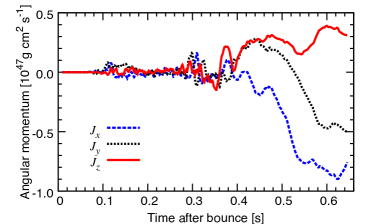
Figure 14: Left: Angular momentum advected onto the PNS calculated according to Equation 5. Right: Evolution of the PNS spin period assuming the moment of inertia of cold neutron stars given by Equation 6.

4 Summary and discussions

We have evolved the binary progenitor model of SN 1987A (Urushibata et al., 2018) in 3D with the neutrino-hydrodynamics code 3DnSNe. The considered stellar model is constructed as a SN 1987A progenitor based on the slow merger scenario and it satisfies most of the observed features like the surface N/C ratio, timing of the blueward evolution of $2\times 10^{4}$ yr before the collapse, and the red-to-blue evolution.

We have found that a shock formed after the core bounce is once stalled at $r\sim 150$ km, and then effective neutrino heating drives anisotropic matter motions behind the shock. The ratio of the advection timescale to the neutrino heating timescale exceeds unity at $\sim 200$ ms and the shock turns to expand at 220 ms after bounce. The expanding shock is roughly spherical, but the matter behind the shock is characterized by a few large hot bubbles going outward.

We have also found that anisotropic motions develop after $\sim 150$ ms post bounce in and out of the PNS. The outer anisotropic motion appears at $\sim 80$ km and gradually spreads outward. At $\sim 260$ ms it merges with post-shock turbulence and the stalled shock turns to expand. The inner anisotropic motion emerges at $\sim 20$ km and it helps transport of neutrinos diffused from the central core of the PNS. Specifically, it enhances the heavy-lepton neutrino luminosity compared to the 1D model without anisotropy. On the other hand, the luminosity of electron-type neutrino ($\nu_{\rm e}$ and $\bar{\nu}_{\rm e}$) is lower in 3D than in 1D, mainly caused by successful shock revival and suppression of accretion onto the central region in the 3D model.

In our supernova model, we have observed non-spherical lepton-number flux called LESA. The multipole ($l\geq 3$) moments evolve first and shift to the dipole and quadrupole moments. This is in line with the findings by Glas et al. (2019), who identified such asymmetry of lepton-number emission and found a similar time-evolution for 9 and 20 $M_{\odot}$ progenitors using different neutrino transport schemes.

We have examined the detectability of neutrino and GW signals assuming the distance to the SN event to be 10 kpc. Super-Kamiokande can detect enough numbers of anti-electron neutrino to determine the time of core bounce as well as the time of shock revival. Catching GW signals from CCSNe is rather difficult but the current detectors (KAGRA, advanced LIGO, and advanced Virgo) could detect not only the strong high-frequency ($>500$ Hz) component but also the relatively weak low-frequency (200–300 Hz) signals from the PNS convection. Our SN 1987A model leaves a PNS with baryonic mass of $1.53\,M_{\odot}$, a kick velocity of $\sim 70\,{\rm km\,s}^{-1}$, and a spin period of $\sim 0.1$ s. Although the central remnant of SN 1987A is not yet confirmed, these PNS properties are in the range of typical NSs.

Our self-consistent 3D simulation demonstrates a neutrino-driven shock revival, but the explosion with a diagnostic explosion energy $\sim 0.14\times 10^{51}$ erg and $<0.01\,M_{\odot}$ of ejected ⁵⁶Ni is very weak compared to the observed properties ($1.5\times 10^{51}$ erg and $0.07\,M_{\odot}$). Although 3D CCSN models usually suffer from such a kind of weak explosion problem, Bollig et al. (2021) reported that they have attained $\sim 10^{51}$ erg explosion energy and $0.087\,M_{\odot}$ Ni mass by means of a modern 3D supernova simulation for the first time. They initiated simulations from the non-spherical progenitor model (see, also Yoshida et al., 2019; Yadav et al., 2020; Yoshida et al., 2021; Varma & Müller, 2021; Fields & Couch, 2021) which is expected to favor large-scale instabilities, and the cycle of continuous downflows and outflows of neutrino-heated matter even after the shock revival led to a monotonic rise of the explosion energy from $\sim 10^{50}$ erg at 0.6 s, as small as our 3D model, up to $\sim 10^{51}$ erg at 7 s after bounce. On the other hand, our simulations start from a spherical progenitor. In our 3D model, small-scale convective flows dominate the matter motions behind the shock. It results in weak accretion flows behind the shock and a small growth rate of the explosion energy. As shown in Figure 8, our 2D model presents a more energetic explosion and produces 4 times more Ni than the 3D model. The 2D model shows a sloshing mode of SASI and the shock is highly aspherical. It leads to an early and vigorous shock revival to the polar direction as well as continuous strong downflows to the proto-NS from the equatorial plane.

There are many works of multi-dimensional CCSN simulations targeted to SN 1987A based on single BSG progenitors (e.g., Kifonidis et al., 2000, 2006; Wongwathanarat et al., 2013, 2015; Utrobin et al., 2015, 2019) and on binary-merger progenitors (Ono et al., 2020; Utrobin et al., 2021). These simulations were performed until minutes, hours, and days so that they can investigate nucleosynthesis and matter mixing in the ejecta. Many important findings consistent with observations, such as the outward mixing of newly formed iron-group elements and inward mixing of hydrogen envelope by Rayleigh-Taylor instabilities at composition interfaces, fast-moving nickel clumps, the distinctive lightcurve of SN 1987A, and implications for the NS kick and spin, have been achieved. Please be aware that the current simulations presented in this paper are intrinsically different from these previous studies. In their simulations, the PNS is excised so that the CFL condition is relaxed, which enables them to perform long-term simulations. In compensation for the simplification, they can not obtain the neutrino property (luminosity and energy distribution). Therefore, they had to assume the PNS contraction rate or the neutrino property itself so that at least one of the observational constraints of SN 1987A (for example, explosion energy) is satisfied. The shortage of the explosion energy and Ni mass in our simulations is suggestive. Long-term simulations including several additional ingredients which are not considered in our simulations such as rotation, magnetic fields, more elaborate neutrino opacity, or even radioactive particle decays like axions (Lucente et al., 2020; Caputo et al., 2021; Caputo et al., 2022; Mori et al., 2022) might produce more energetic 3D CCSN models and help bridging a gap between the observed values and theoretical predictions, which we leave as our future work.

Data Availability

The data underlying this article will be shared on reasonable request to the corresponding author.

References

- Abbar et al. (2019) Abbar S., Duan H., Sumiyoshi K., Takiwaki T., Volpe M. C., 2019, Phys. Rev. D, 100, 043004
- Abdikamalov et al. (2020) Abdikamalov E., Pagliaroli G., Radice D., 2020, arXiv e-prints, p. arXiv:2010.04356
- Alekseev et al. (1987) Alekseev E. N., Alekseeva L. N., Volchenko V. I., Krivosheina I. V., 1987, Soviet Journal of Experimental and Theoretical Physics Letters, 45, 589
- Alexeyev et al. (1988) Alexeyev E. N., Alexeyeva L. N., Krivosheina I. V., Volchenko V. I., 1988, Physics Letters B, 205, 209
- Alp et al. (2018) Alp D., et al., 2018, ApJ, 864, 174
- Andresen et al. (2019) Andresen H., Müller E., Janka H.-T., Summa A., Gill K., Zanolin M., 2019, MNRAS, 486, 2238
- Arnett (1966) Arnett W. D., 1966, Canadian Journal of Physics, 44, 2553
- Arnett (1987) Arnett W. D., 1987, ApJ, 319, 136
- Arnett et al. (1989) Arnett W. D., Bahcall J. N., Kirshner R. P., Woosley S. E., 1989, ARA&A, 27, 629
- Barkat & Wheeler (1989) Barkat Z., Wheeler J. C., 1989, ApJ, 342, 940
- Bear & Soker (2018) Bear E., Soker N., 2018, MNRAS, 478, 682
- Bethe & Wilson (1985) Bethe H. A., Wilson J. R., 1985, ApJ, 295, 14
- Bionta et al. (1987) Bionta R. M., Blewitt G., Bratton C. B., Casper D., Ciocio A., 1987, Physical Review Letters, 58, 1494
- Blanco et al. (1987) Blanco W. M., et al., 1987, ApJ, 320, 589
- Bollig et al. (2021) Bollig R., Yadav N., Kresse D., Janka H.-T., Müller B., Heger A., 2021, ApJ, 915, 28
- Bouchet et al. (1991) Bouchet P., Phillips M. M., Suntzeff N. B., Gouiffes G., Hanuschik R. W., Wooden D. H., 1991, A&A, 245, 490
- Bratton et al. (1988) Bratton C. B., et al., 1988, Phys. Rev. D, 37, 3361
- Buras et al. (2006) Buras R., Rampp M., Janka H.-T., Kifonidis K., 2006, A&A, 447, 1049
- Burrows et al. (1995) Burrows C. J., et al., 1995, ApJ, 452, 680
- Burrows et al. (2020) Burrows A., Radice D., Vartanyan D., Nagakura H., Skinner M. A., Dolence J. C., 2020, MNRAS, 491, 2715
- Caputo et al. (2021) Caputo A., Carenza P., Lucente G., Vitagliano E., Giannotti M., Kotake K., Kuroda T., Mirizzi A., 2021, Phys. Rev. Lett., 127, 181102
- Caputo et al. (2022) Caputo A., Janka H.-T., Raffelt G., Vitagliano E., 2022, arXiv e-prints, p. arXiv:2201.09890
- Catchpole et al. (1988) Catchpole R. M., et al., 1988, MNRAS, 231, 75P
- Chakraborty & Chakraborty (2020) Chakraborty M., Chakraborty S., 2020, J. Cosmology Astropart. Phys., 2020, 005
- Cherry et al. (2020) Cherry J. F., Fuller G. M., Horiuchi S., Kotake K., Takiwaki T., Fischer T., 2020, Phys. Rev. D, 102, 023022
- Cigan et al. (2019) Cigan P., et al., 2019, ApJ, 886, 51
- Colgate & White (1966) Colgate S. A., White R. H., 1966, ApJ, 143, 626
- De Loore & Vanbeveren (1992) De Loore C., Vanbeveren D., 1992, A&A, 260, 273
- Duchêne & Kraus (2013) Duchêne G., Kraus A., 2013, ARA&A, 51, 269
- Eggenberger Andersen et al. (2021) Eggenberger Andersen O., Zha S., da Silva Schneider A., Betranhandy A., Couch S. M., O’Connor E. P., 2021, arXiv e-prints, p. arXiv:2106.09734
- Enoto et al. (2019) Enoto T., Kisaka S., Shibata S., 2019, Reports on Progress in Physics, 82, 106901
- Esposito et al. (2018) Esposito P., Rea N., Lazzati D., Matsuura M., Perna R., Pons J. A., 2018, ApJ, 857, 58
- Fabian et al. (1987) Fabian A. C., Rees M. J., van den Heuvel E. P. J., van Paradijs J., 1987, Nature, 328, 323
- Fields & Couch (2021) Fields C. E., Couch S. M., 2021, ApJ, 921, 28
- France et al. (2010) France K., et al., 2010, Science, 329, 1624
- Fryer & Heger (2000) Fryer C. L., Heger A., 2000, ApJ, 541, 1033
- Glas et al. (2019) Glas R., Janka H. T., Melson T., Stockinger G., Just O., 2019, ApJ, 881, 36
- Hachisu et al. (1990) Hachisu I., Matsuda T., Nomoto K., Shigeyama T., 1990, ApJ, 358, L57
- Hamuy et al. (1988) Hamuy M., Suntzeff N. B., Gonzalez R., Martin G., 1988, AJ, 95, 63
- Harada & Nagakura (2022) Harada A., Nagakura H., 2022, ApJ, 924, 109
- Hillebrandt & Meyer (1989) Hillebrandt W., Meyer F., 1989, A&A, 219, L3
- Hillebrandt et al. (1987) Hillebrandt W., Hoeflich P., Weiss A., Truran J. W., 1987, Nature, 327, 597
- Hirata et al. (1987) Hirata K., Kajita T., Koshiba M., Nakahata M., Oyama Y., 1987, Physical Review Letters, 58, 1490
- Hirata et al. (1988) Hirata K. S., et al., 1988, Phys. Rev. D, 38, 448
- Horiuchi & Kneller (2018) Horiuchi S., Kneller J. P., 2018, Journal of Physics G Nuclear Physics, 45, 043002
- Ivanova et al. (2002) Ivanova N., Podsiadlowski P., Spruit H., 2002, MNRAS, 334, 819
- Iwakami et al. (2020) Iwakami W., Okawa H., Nagakura H., Harada A., Furusawa S., Sumiyoshi K., Matsufuru H., Yamada S., 2020, ApJ, 903, 82
- Janka et al. (2016) Janka H.-T., Melson T., Summa A., 2016, Annual Review of Nuclear and Particle Science, 66, 341
- Jerkstrand et al. (2020) Jerkstrand A., et al., 2020, MNRAS, 494, 2471
- Joss et al. (1988) Joss P. C., Podsiadlowski P., Hsu J. J. L., Rappaport S., 1988, Nature, 331, 237
- Kato et al. (2020) Kato C., Nagakura H., Hori Y., Yamada S., 2020, ApJ, 897, 43
- Kato et al. (2021) Kato C., Nagakura H., Morinaga T., 2021, ApJS, 257, 55
- Kifonidis et al. (2000) Kifonidis K., Plewa T., Janka H. T., Müller E., 2000, ApJ, 531, L123
- Kifonidis et al. (2006) Kifonidis K., Plewa T., Scheck L., Janka H.-T., Müller E., 2006, A&A, 453, 661
- Kitaura et al. (2006) Kitaura F. S., Janka H. T., Hillebrandt W., 2006, A&A, 450, 345
- Kotake (2013) Kotake K., 2013, Comptes Rendus Physique, 14, 318
- Kotake et al. (2006) Kotake K., Sato K., Takahashi K., 2006, Reports on Progress in Physics, 69, 971
- Kotake et al. (2018) Kotake K., Takiwaki T., Fischer T., Nakamura K., Martínez-Pinedo G., 2018, ApJ, 853, 170
- Kumagai et al. (1988) Kumagai S., Itoh M., Shigeyama T., Nomoto K., Nishimura J., 1988, A&A, 197, L7
- Kumagai et al. (1989) Kumagai S., Shigeyama T., Nomoto K., Itoh M., Nishimura J., Tsuruta S., 1989, ApJ, 345, 412
- Kuroda et al. (2016) Kuroda T., Kotake K., Takiwaki T., 2016, ApJ, 829, L14
- Langer (1991) Langer N., 1991, A&A, 243, 155
- Langer et al. (1989) Langer N., El Eid M. F., Baraffe I., 1989, A&A, 224, L17
- Laplace et al. (2021) Laplace E., Justham S., Renzo M., Götberg Y., Farmer R., Vartanyan D., de Mink S. E., 2021, A&A, 656, A58
- Larsson et al. (2013) Larsson J., et al., 2013, ApJ, 768, 89
- Lattimer & Swesty (1991) Lattimer J. M., Swesty F. D., 1991, Nuclear Physics A, 535, 331
- Lentz et al. (2015) Lentz E. J., et al., 2015, ApJ, 807, L31
- Liebendörfer et al. (2001) Liebendörfer M., Mezzacappa A., Thielemann F.-K., Messer O. E., Hix W. R., Bruenn S. W., 2001, Phys. Rev. D, 63, 103004
- Liebendörfer et al. (2009) Liebendörfer M., Whitehouse S. C., Fischer T., 2009, ApJ, 698, 1174
- Lucente et al. (2020) Lucente G., Carenza P., Fischer T., Giannotti M., Mirizzi A., 2020, J. Cosmology Astropart. Phys., 2020, 008
- Lundqvist & Fransson (1996) Lundqvist P., Fransson C., 1996, ApJ, 464, 924
- Maeder (1987) Maeder A., 1987, in European Southern Observatory Conference and Workshop Proceedings. p. 251
- Marek et al. (2006) Marek A., Dimmelmeier H., Janka H. T., Müller E., Buras R., 2006, A&A, 445, 273
- Matsumoto et al. (2020) Matsumoto J., Takiwaki T., Kotake K., Asahina Y., Takahashi H. R., 2020, MNRAS, 499, 4174
- Matsumoto et al. (2022) Matsumoto J., Asahina Y., Takiwaki T., Kotake K., Takahashi H. R., 2022, arXiv e-prints, p. arXiv:2202.07967
- Mattila et al. (2010) Mattila S., Lundqvist P., Gröningsson P., Meikle P., Stathakis R., Fransson C., Cannon R., 2010, ApJ, 717, 1140
- McCray (1993) McCray R., 1993, ARA&A, 31, 175
- McCray & Fransson (2016) McCray R., Fransson C., 2016, ARA&A, 54, 19
- Melson et al. (2015a) Melson T., Janka H.-T., Marek A., 2015a, ApJ, 801, L24
- Melson et al. (2015b) Melson T., Janka H.-T., Bollig R., Hanke F., Marek A., Müller B., 2015b, ApJ, 808, L42
- Menon & Heger (2017) Menon A., Heger A., 2017, MNRAS, 469, 4649
- Menon et al. (2019) Menon A., Utrobin V., Heger A., 2019, MNRAS, 482, 438
- Mezzacappa et al. (2020) Mezzacappa A., et al., 2020, Phys. Rev. D, 102, 023027
- Mirizzi et al. (2016) Mirizzi A., Tamborra I., Janka H.-T., Saviano N., Scholberg K., Bollig R., Hüdepohl L., Chakraborty S., 2016, Nuovo Cimento Rivista Serie, 39, 1
- Mori et al. (2021) Mori M., Suwa Y., Nakazato K., Sumiyoshi K., Harada M., Harada A., Koshio Y., Wendell R. A., 2021, Progress of Theoretical and Experimental Physics, 2021, 023E01
- Mori et al. (2022) Mori K., Takiwaki T., Kotake K., Horiuchi S., 2022, Phys. Rev. D, 105, 063009
- Morozova et al. (2018) Morozova V., Radice D., Burrows A., Vartanyan D., 2018, ApJ, 861, 10
- Müller & Varma (2020) Müller B., Varma V., 2020, MNRAS, 498, L109
- Müller et al. (2018) Müller B., Gay D. W., Heger A., Tauris T. M., Sim S. A., 2018, MNRAS, 479, 3675
- Müller et al. (2019) Müller B., et al., 2019, MNRAS, 484, 3307
- Nagakura & Vartanyan (2021) Nagakura H., Vartanyan D., 2021, arXiv e-prints, p. arXiv:2111.05869
- Nagakura et al. (2019) Nagakura H., Sumiyoshi K., Yamada S., 2019, ApJ, 880, L28
- Nagakura et al. (2020) Nagakura H., Burrows A., Radice D., Vartanyan D., 2020, MNRAS, 492, 5764
- Nagakura et al. (2021a) Nagakura H., Burrows A., Johns L., Fuller G. M., 2021a, Phys. Rev. D, 104, 083025
- Nagakura et al. (2021b) Nagakura H., Burrows A., Vartanyan D., Radice D., 2021b, MNRAS, 500, 696
- Nagakura et al. (2021c) Nagakura H., Burrows A., Vartanyan D., 2021c, MNRAS, 506, 1462
- Nagataki (2000) Nagataki S., 2000, ApJS, 127, 141
- Nakamura et al. (2014) Nakamura K., Takiwaki T., Kotake K., Nishimura N., 2014, ApJ, 782, 91
- Nakamura et al. (2016) Nakamura K., Horiuchi S., Tanaka M., Hayama K., Takiwaki T., Kotake K., 2016, MNRAS, 461, 3296
- Nakamura et al. (2019) Nakamura K., Takiwaki T., Kotake K., 2019, PASJ, 71, 98
- Nakazato & Suzuki (2019) Nakazato K., Suzuki H., 2019, ApJ, 878, 25
- Nakazato et al. (2021) Nakazato K., Sumiyoshi K., Togashi H., 2021, PASJ, 73, 639
- Nakazato et al. (2022) Nakazato K., et al., 2022, ApJ, 925, 98
- Nordhaus et al. (2010) Nordhaus J., Burrows A., Almgren A., Bell J., 2010, ApJ, 720, 694
- O’Connor & Ott (2011) O’Connor E., Ott C. D., 2011, ApJ, 730, 70
- Ono et al. (2020) Ono M., Nagataki S., Ferrand G., Takahashi K., Umeda H., Yoshida T., Orlando S., Miceli M., 2020, ApJ, 888, 111
- Ott et al. (2018) Ott C. D., Roberts L. F., da Silva Schneider A., Fedrow J. M., Haas R., Schnetter E., 2018, ApJ, 855, L3
- Page et al. (2020) Page D., Beznogov M. V., Garibay I., Lattimer J. M., Prakash M., Janka H.-T., 2020, ApJ, 898, 125
- Pietrzyński et al. (2019) Pietrzyński G., et al., 2019, Nature, 567, 200
- Podsiadlowski (1992) Podsiadlowski P., 1992, PASP, 104, 717
- Podsiadlowski & Joss (1989) Podsiadlowski P., Joss P. C., 1989, Nature, 338, 401
- Podsiadlowski et al. (1990) Podsiadlowski P., Joss P. C., Rappaport S., 1990, A&A, 227, L9
- Podsiadlowski et al. (1992) Podsiadlowski P., Joss P. C., Hsu J. J. L., 1992, ApJ, 391, 246
- Radice et al. (2019) Radice D., Morozova V., Burrows A., Vartanyan D., Nagakura H., 2019, ApJ, 876, L9
- Richers et al. (2021) Richers S., Willcox D., Ford N., 2021, Phys. Rev. D, 104, 103023
- Saio et al. (1988) Saio H., Kato M., Nomoto K., 1988, ApJ, 331, 388
- Sana et al. (2013) Sana H., et al., 2013, A&A, 550, A107
- Sasaki & Takiwaki (2021) Sasaki H., Takiwaki T., 2021, arXiv e-prints, p. arXiv:2109.14011
- Sasaki et al. (2020) Sasaki H., Takiwaki T., Kawagoe S., Horiuchi S., Ishidoshiro K., 2020, Phys. Rev. D, 101, 063027
- Sato & Suzuki (1987) Sato K., Suzuki H., 1987, Physical Review Letters, 58, 2722
- Sawada & Maeda (2019) Sawada R., Maeda K., 2019, ApJ, 886, 47
- Sawada & Suwa (2021) Sawada R., Suwa Y., 2021, ApJ, 908, 6
- Scheck et al. (2006) Scheck L., Kifonidis K., Janka H.-T., Müller E., 2006, A&A, 457, 963
- Seitenzahl et al. (2014) Seitenzahl I. R., Timmes F. X., Magkotsios G., 2014, ApJ, 792, 10
- Shalgar & Tamborra (2019) Shalgar S., Tamborra I., 2019, ApJ, 883, 80
- Shalgar & Tamborra (2021) Shalgar S., Tamborra I., 2021, Phys. Rev. D, 104, 023011
- Shibagaki et al. (2020) Shibagaki S., Kuroda T., Kotake K., Takiwaki T., 2020, MNRAS, 493, L138
- Shibagaki et al. (2021) Shibagaki S., Kuroda T., Kotake K., Takiwaki T., 2021, Characteristic time variability of gravitational-wave and neutrino signals from three-dimensional simulations of non-rotating and rapidly rotating stellar core collapse (arXiv:2010.03882), doi:10.1093/mnras/stab228
- Shigeyama & Nomoto (1990) Shigeyama T., Nomoto K., 1990, ApJ, 360, 242
- Shigeyama et al. (1988) Shigeyama T., Nomoto K., Hashimoto M., 1988, A&A, 196, 141
- Sigl (2022) Sigl G., 2022, Phys. Rev. D, 105, 043005
- Sotani & Takiwaki (2020a) Sotani H., Takiwaki T., 2020a, Phys. Rev. D, 102, 063025
- Sotani & Takiwaki (2020b) Sotani H., Takiwaki T., 2020b, MNRAS, 498, 3503
- Sotani et al. (2017) Sotani H., Kuroda T., Takiwaki T., Kotake K., 2017, Phys. Rev. D, 96, 063005
- Stockinger et al. (2020) Stockinger G., et al., 2020, MNRAS, 496, 2039
- Sumiyoshi et al. (2005) Sumiyoshi K., Yamada S., Suzuki H., Shen H., Chiba S., Toki H., 2005, ApJ, 629, 922
- Summa et al. (2018) Summa A., Janka H.-T., Melson T., Marek A., 2018, ApJ, 852, 28
- Suntzeff & Bouchet (1990) Suntzeff N. B., Bouchet P., 1990, AJ, 99, 650
- Suwa et al. (2019) Suwa Y., Sumiyoshi K., Nakazato K., Takahira Y., Koshio Y., Mori M., Wendell R. A., 2019, ApJ, 881, 139
- Suwa et al. (2021) Suwa Y., Harada A., Nakazato K., Sumiyoshi K., 2021, Progress of Theoretical and Experimental Physics, 2021, 013E01
- Takiwaki & Kotake (2018) Takiwaki T., Kotake K., 2018, MNRAS, 475, L91
- Takiwaki et al. (2012) Takiwaki T., Kotake K., Suwa Y., 2012, ApJ, 749, 98
- Takiwaki et al. (2014) Takiwaki T., Kotake K., Suwa Y., 2014, ApJ, 786, 83
- Takiwaki et al. (2016) Takiwaki T., Kotake K., Suwa Y., 2016, MNRAS, 461, L112
- Takiwaki et al. (2021) Takiwaki T., Kotake K., Foglizzo T., 2021, MNRAS, 508, 966
- Tamborra et al. (2014) Tamborra I., Hanke F., Janka H.-T., Müller B., Raffelt G. G., Marek A., 2014, ApJ, 792, 96
- Torres-Forné et al. (2019) Torres-Forné A., Cerdá-Durán P., Passamonti A., Obergaulinger M., Font J. A., 2019, MNRAS, 482, 3967
- Urushibata et al. (2018) Urushibata T., Takahashi K., Umeda H., Yoshida T., 2018, MNRAS, 473, L101
- Utrobin et al. (2015) Utrobin V. P., Wongwathanarat A., Janka H. T., Müller E., 2015, A&A, 581, A40
- Utrobin et al. (2019) Utrobin V. P., Wongwathanarat A., Janka H. T., Müller E., Ertl T., Woosley S. E., 2019, A&A, 624, A116
- Utrobin et al. (2021) Utrobin V. P., Wongwathanarat A., Janka H. T., Müller E., Ertl T., Menon A., Heger A., 2021, ApJ, 914, 4
- Varma & Müller (2021) Varma V., Müller B., 2021, MNRAS, 504, 636
- Vartanyan et al. (2019) Vartanyan D., Burrows A., Radice D., Skinner M. A., Dolence J., 2019, MNRAS, 482, 351
- Vartanyan et al. (2021) Vartanyan D., Laplace E., Renzo M., Götberg Y., Burrows A., de Mink S. E., 2021, ApJ, 916, L5
- Walborn et al. (1987) Walborn N. R., Lasker B. M., Laidler V. G., Chu Y.-H., 1987, ApJ, 321, L41
- Wampler & Richichi (1989) Wampler E. J., Richichi A., 1989, A&A, 217, 31
- Wampler et al. (1990) Wampler E. J., Wang L., Baade D., Banse K., D’Odorico S., Gouiffes C., Tarenghi M., 1990, ApJ, 362, L13
- Wang et al. (2002) Wang L., et al., 2002, ApJ, 579, 671
- Weiss (1989) Weiss A., 1989, ApJ, 339, 365
- Weiss et al. (1988) Weiss A., Hillebrandt W., Truran J. W., 1988, A&A, 197, L11
- Wongwathanarat et al. (2010) Wongwathanarat A., Hammer N. J., Müller E., 2010, A&A, 514, A48
- Wongwathanarat et al. (2013) Wongwathanarat A., Janka H.-T., Müller E., 2013, A&A, 552, A126
- Wongwathanarat et al. (2015) Wongwathanarat A., Müller E., Janka H. T., 2015, A&A, 577, A48
- Wood & Faulkner (1987) Wood P. R., Faulkner D. J., 1987, Proceedings of the Astronomical Society of Australia, 7, 75
- Woosley & Heger (2007) Woosley S. E., Heger A., 2007, Phys. Rep., 442, 269
- Woosley et al. (1988) Woosley S. E., Pinto P. A., Ensman L., 1988, ApJ, 324, 466
- Yadav et al. (2020) Yadav N., Müller B., Janka H. T., Melson T., Heger A., 2020, ApJ, 890, 94
- Yoshida et al. (2019) Yoshida T., Takiwaki T., Kotake K., Takahashi K., Nakamura K., Umeda H., 2019, arXiv e-prints,
- Yoshida et al. (2021) Yoshida T., Takiwaki T., Aguilera-Dena D. R., Kotake K., Takahashi K., Nakamura K., Umeda H., Langer N., 2021, MNRAS, 506, L20
- Zaizen et al. (2021) Zaizen M., Horiuchi S., Takiwaki T., Kotake K., Yoshida T., Umeda H., Cherry J. F., 2021, Phys. Rev. D, 103, 063008