Thermodynamic and Optical Behaviors
of Quintessential Hayward-AdS Black Holes

Abstract

Motivated by Dark Energy (DE) activities, we study certain physical behaviors of the quintessential Hayward-AdS black holes in four dimensions. We generalize some physical properties of the ordinary Hayward AdS black holes without the dark sector. We elaborate a study in terms of the new quantities $c$ and $\omega_{q}$ parametrizing the dark sector moduli space. We investigate the effect of such parameters on certain thermodynamic and optical aspects. To show the quintessential thermodynamic behaviors, we first reconsider the critical properties of the ordinary solutions. We find that the equation of state predicts a universal ratio given by $\chi_{0}=\frac{P_{c}v_{c}}{T_{c}}=\frac{27-3\sqrt{6}}{50}$, which is different than the universal one appearing for Van der Waals fluids. Considering the quintessential solutions and taking certain values of the DE state parameter $\omega_{q}$, we observe that the new ratio depends on the DE scalar field intensity $c$. In certain regions of the moduli space, we show that this ratio can be factorized using two terms describing the absence and the presence of the dark sector. Then, we analyze also the DE effect on the heat engines. For the optical aspect, we study the influence of DE on the shadows using one dimensional real curves. Finally, we discuss the associated energy emission rate, using the dark sector.

Keywords: Hayward-AdS black holes, Dark energy, Thermodynamics, Heat engine, Shadow optical behavior.

1 Introduction

Recently, the phase structure of the Anti de Sitter (AdS) black holes has received more attention from the extended phase space point of views [1, 2]. In such an extended space, it has been implemented both the pressure and the volume as thermodynamic variables [3]. Various interesting phenomena of the AdS black holes have been explored, such as reentrant phase transitions[4, 12], triple points [13], and $\lambda$-line phase transitions [14]. These activities have suggested that the AdS black holes offer huge similarities with the thermodynamic systems.
It has been remarked that the investigation of the black hole singularities has always been a real crisis in general relativity theory. The singularities are considered as serious problems in such a theory[5, 6, 7, 8, 9, 10, 11]. To overcome such issues, many suggestions have been proposed. In particular, regular black hole solutions have been elaborated. Among others, the theory of general relativity coupled to nonlinear electrodynamics has been also considered as an interesting candidate [15, 16]. Alternative ways generate regular solutions containing a critical scale, mass, and charge parameters restricted by certain values, depending only on the type of the curvature invariants [17]. Hayward presented a static spherically symmetric black hole being near the origin behaves like a de Sitter space-time. Precisely, its curvature is invariant everywhere and satisfies the weak energy condition[18]. Several Hayward-like black holes have been constructed after the original one by introducing an irregularity to topological changes. This offers a possibility to build spaces with a maximum curvature inside the black hole regions [19, 20, 21]. Regular black hole interior solutions have been also found in Loop Quantum Gravity [22]. In particular, they represent relevant ingredients needed to understand the associated physical theories.
In addition to the singularity problems, the general relativity theory should resolve certain questions which remain without a consensus. These questions may concern the dark sector associated with the dark matter [23] and the dark energy of late-time cosmology[24]. As a way to investigate the models dealing with such as a sector, a scalar field is usually introduced [25, 26]. Concretely, the quintessence remains the simplest and the promising one [27, 28, 29]. Recently, it has been shown that the observational results could confirm that our universe is expanding with acceleration behaviors[30, 31]. It has been remarked that this surprisingly accelerated expansion can be explained by the introduction of the dark energy, which accounts about 70% of the universe. It involves a negative pressure driving the expansion of the universe. Precisely, it has been suggested that such an energy could be modeled, in terms of a quintessential scalar field being considered as a spatially homogeneous real scalar field with intensity $c$. Treated as a perfect fluid with a pressure $p$ and an energy density $\rho_{q}$, such a DE is controlled by the equation of state $p=\omega_{q}\rho_{q}$ where $\omega_{q}$ is called a state parameter with the constraint $-1<\omega_{q}<-{1}/{3}$.
Kiselev first derived the solutions of the black hole in the presence of the quintessence[32]. Following this work, many black holes surrounded by the quintessential dark fields have been dealt with by unveiling certain data of the associated physics[33, 34, 35, 36].
Beside phase transitions and critical phenomena, developments in the black hole thermodynamics have provided many works including the Joule-Thomson expansion [37, 38] and the holographic heat engine behaviors [40, 39, 41, 42]. Considering the AdS black holes as heat engines, various black holes have been examined. Concretely, the ordinary Hayward AdS black holes without external moduli space have been studied in [3, 43]. The effect of DE on engine behaviors for RN-AdS black holes have been elaborated in [44]. It has been shown that the quintessence, controlled by an external moduli space, could improve the associated efficiency. A close inspection has revealed that DE affects also the optical aspect which has been dealt with using the shadow geometries in terms of one dimensional real curves. For certain black holes solutions, DE can be considered as a geometric deformation parameter controlling the size of the shadows [36, 45, 46, 47, 48, 49].

The aim of this work is to contribute to such activities by investigating physical behaviors of the quintessential Hayward-AdS black holes in four dimensions. In particular, we generalize certain physical properties of the ordinary Hayward AdS black holes without external moduli space associated with the dark sector. We elaborate a study in terms of the new quantities $c$ and $\omega_{q}$ parametrizing the dark sector moduli space. Precisely, we study the effect of such parameters on certain thermodynamic and optical aspects. Before examining the quintessential thermodynamic behaviors, we first reconsider the critical properties of the ordinary solutions associated with $c=0$. We find that the equation of state predicts a universal ratio given by $\chi_{0}=\frac{P_{c}v_{c}}{T_{c}}=\frac{27-3\sqrt{6}}{50}$. This ration is different than the universal one found for Van der Waals fluids. Considering the quintessential solutions and taking certain values of the DE state parameter $\omega_{q}$, we remark that the new ratio depends on the DE field intensity $c$. In certain regions of the moduli space, we show that this ratio can be factorized using two parts describing the absence and the presence of the dark sector. By considering models associated with $\omega_{q}=-1,-\frac{1}{3},-\frac{2}{3}$, we analyze also the DE effect on the heat engine behaviors of such black holes. Putting $c=0$, we recover the previous results corresponding to the ordinary solutions. For the optical aspect, we examine the effect of DE on the shadows in terms of one dimensional real curves. We find that DE contributions deform the shadow radius. Finally, we discuss the associated energy emission rate using the dark sector.

This work is organized as follows. In section 2, we reconsider the study of the critical behaviors of the quintessential Hayward-AdS black holes in four dimensions. In section 3, we investigate the effect of DE on such black holes as heat engines. In section 4, we examine the associated optical behaviors by considering shadow geometries using one dimensional real closed curves, and the associated energy emission. In the last section, we give conclusions and final remarks.

2 The model: Quintessential Hayward-AdS Black Hole

It has been suggested that black holes in scalar field backgrounds could provide concrete and semi-realistic models in connections with cosmological findings. An examination shows that many scalar models have been introduced supported by non-trivial theories including M-theory and superstrings. This could produce black holes with external parameters describing the scalar field sector. The later has been approached from different angles. The most exotic models are the dynamic dark energy models modeled in terms of a scalar field. It turns out that there are several types of scalar field theories including the quintessence model. It has been shown that this model can be considered as a cooling system. This result pushes one to inspect the effect of such an energy on the other physical properties including the thermodynamical and optical ones.

The models that we would like to elaborate are the quintessential AdS black holes in four dimensions. In the simplest model, the quintessential DE could be formulated in terms of a scalar field minimally coupled to gravity describing the ordinary AdS black hole solutions. Concretely, a close examination reveals that the moduli space of such AdS black holes can be factorized in two sectors

$$\mathcal{M}=\mathcal{M}_{obh}\times\mathcal{M}_{ds}$$ (2.1)

The first sector corresponds to the parameters of the ordinary AdS balck holes (obh)

$$\mathcal{M}_{obh}=\{M,a,Q,\Lambda\}$$ (2.2)

where $a$ is the rotating parameter and $\Lambda$ is the cosmological constant. $M$ and $Q$ are the mass and charge parameters, respectively. For the non-rotating black hole $(a=0)$, this can be reduced to a black hole moduli space parameterized only by $M$, $Q$ and $\Lambda$

$$\mathcal{M}_{obh}=\{M,Q,\Lambda\}.$$ (2.3)

The second sector $\mathcal{M}_{ds}$ that we are interested in represents the extra contributions corresponding to outside horizon contributions including DE, DM and other non trivial ones. Here, we consider only DE contributions via a quintessence scalar field. In this way, the dark sector can be controlled by two parameters $c$ and $\omega_{q}$ associated with the quintessence intensity and the DE state parameter, respectively. In this way, we can write

$$\mathcal{M}_{ds}=\{c,\omega_{q}\}.$$ (2.4)

For generic values of $c$, a close examination shows that the associated black hole models should depend only on $\omega_{q}$. In the present work, however, we pay attention to certain particular cases. General values of such a DE state parameter may need non trivial reflections to analyze the corresponding thermodynamic and optical behaviors in the presence of the quintessence. This contribution can be considered as an alternative contribution to the cosmological constant where the equation of state could take a central place. Many models of such energy contributions have been dealt with including ones describing a possible deviation of the cosmological constant via a single scalar field. In this way, the equation of state parameter can be toke as the following form

$$\omega_{q}=-1+\frac{2}{3}\epsilon_{\phi}$$ (2.5)

where $\epsilon_{\phi}$ indicates a positive contribution obtained from the scalar potential associated with the quintessence. In cosmological models, $\epsilon_{\phi}$ has been called slow-roll parameter. Certain models could be examined using scalar potentials already investigated in the literature. The selection of such scalar models has not been an easy task. In connection with black holes, three models have been extensively studied corresponding to three values of $\epsilon_{\phi}$ being 0, $\frac{1}{2}$, and 1 giving $\omega_{q}=-1,-\frac{2}{3},-\frac{1}{3}$. Assuming that the spacetime metric is static, spheric and symmetric, the line element describing such non rotating AdS black holes should be written as

$$ds^{2}=-f_{\omega_{q}}(r)dt^{2}+\frac{dr^{2}}{f_{\omega_{q}}(r)}+r^{2}d\Omega^{2},$$ (2.6)

where $f_{\omega_{q}}$ is the quintessential black hole metric function and $d\Omega^{2}$ is the line element of the 2-dimensional unit sphere. This function, which contains information on the above factorized moduli space, can be written as

$$f_{\omega_{q}}(r)=f(r)+cg(r)$$ (2.7)

where $g(r)$ is a function which depends on the dark sector state equation. Taking $c=0$, we can recover the ordinary the AdS Black Holes described by the metric function $f$. The main objective of this paper is to inspect the influence of the dark sector moduli space $\mathcal{M}_{ds}$ on physical properties of the ordinary Hayward AdS black holes. In particular, we study DE effects in terms of the new parameters associated with such a sector. At particular points of the moduli spaces, we will show that certain thermodynamical quantities $X_{c}$ can be factorized according the above metric function as follows

$$X_{c}\sim X_{0}+cX$$ (2.8)

where $X$ is an extra contribution associated with the dark sector. Similar optical behaviors will be shown.

3 Thermodynamic behaviors of Hayward-AdS black hole from DE

In this section, we investigate the effect of DE on critical behaviors of the Hayward-AdS black holes in four dimensions. Before studying such models, we reconsider the study of the ordinary solutions without DE contributions. In particular, we investigate the critical aspect.

3.1 Criticality behaviors of ordinary black hole solutions

In this part, we investigate the criticality behaviors of the proposed black hole solutions without DE contributions. For generic charge values, we first show that the ordinary solutions involve a critical universal ratio. Precisely, the equation of state for the quintessential black holes predicts a critical universal ratio depending on the involved DE fields. To reveal that, we consider the ordinary solutions associated with the Hayward-AdS metric [50]. We start by taking the following action

$$S=\frac{1}{16\pi}\int d^{4}x\sqrt{-g}\left(R-2\Lambda-\mathcal{L}(\mathcal{F})\right),$$ (3.1)

where one has used $\mathcal{F}=F_{\mu\nu}F^{\mu\nu}$. Here, $\mathcal{L}$ is a Lagrangian density depending only on $\mathcal{F}$ and $\Lambda=-\frac{3}{\ell^{2}}$. Varying the action with respect to the metric tensor $g_{\mu\nu}$ and the field strength $F_{\mu\nu}$, one gets the following equations of motion

$$G_{\mu\nu}-\frac{3}{\ell^{2}}g_{\mu\nu}=T_{\mu\nu},\quad\quad\nabla_{\mu}\left(\mathcal{L}_{\mathcal{F}}F^{\mu\nu}\right)=0$$ (3.2)

with $\mathcal{L}_{\mathcal{F}}=\frac{\partial\mathcal{L}(\mathcal{F})}{\partial\mathcal{F}}$ and $T_{\mu\nu}=2\left(\mathcal{L}_{\mathcal{F}}F_{\mu\nu}^{2}-\frac{1}{4}g_{\mu\nu}\mathcal{L}\right).$ For $c=0$, the spacetime metric has the following line element

$$ds^{2}=-f(r)dt^{2}+\frac{dr^{2}}{f(r)}+r^{2}d\Omega^{2}.$$ (3.3)

Using the above equations, we can obtain the $(t,t)$ component metric giving

$$\frac{rf^{\prime}(r)+f(r)-1}{r^{2}}-\frac{3}{\ell^{2}}=-\frac{\mathcal{L}(\mathcal{F})}{2}.$$ (3.4)

In terms of the mass parameter, this can be written as

$$\frac{2m^{\prime}(r)}{r^{2}}+\frac{3}{\ell^{2}}=\frac{\mathcal{L}(\mathcal{F})}{2}.$$ (3.5)

The associated calculation can be carried out according to the work reported in [60]. In particular, we consider the Lagrangian density given by

$$\mathcal{L}(\mathcal{F})=\frac{4\mu}{\alpha}\frac{\left(\alpha\mathcal{F}\right)^{5/4}}{\left(1+\sqrt{\alpha\mathcal{F}}\right)^{1+\frac{\mu}{2}}}$$ (3.6)

where one has $\mathcal{F}=\frac{2q_{m}^{2}}{r^{4}}$. $\alpha$ is a constant satisfying $\alpha=\frac{Q^{4}}{2q_{m}^{2}}$. $\mu$ is a positive dimensionless constant. It is recalled that Hayward black hole can be recovered by taking $\mu=3$ and $\alpha^{-1}Q^{3}=M$. After certain calculations, one can obtain

$$m(r)=-\frac{8Mq_{m}^{6}}{8q_{m}^{6}+M^{3}r^{3}}+C_{1}-\frac{r^{3}}{2\ell^{2}},$$ (3.7)

where $C_{1}$ is an integration constant and where $M$ is the black hole mass parameter. Many solutions could be obtained by taking certain limits. Here, we consider $f(r)$ which is a relevant function known by the metric function taking the following form

$$f(r)=1+\frac{r^{2}}{\ell^{2}}-\frac{2Mr^{2}}{r^{3}+Q^{3}},$$ (3.8)

where $\ell$ represents the AdS length. It is noted that the parameter $Q$ is related to the total magnetic charge $q_{m}$ via the relation

$$q_{m}=\frac{Q^{2}}{\sqrt{2a}}$$ (3.9)

where $a$ is a free integration constant. In thermodynamical activities of the AdS black holes, the cosmological constant $\Lambda=-\frac{3}{\ell^{2}}$ has been interpreted as the pressure

$$P=-\frac{\Lambda}{8\pi}=\frac{3}{8\pi\ell^{2}},$$ (3.10)

and its conjugate variable is associated with the thermodynamic volume. The black hole mass $M$ can be obtained by solving the constraint $f(r)=0$. The computations give

$$M=\frac{\left(Q^{3}+r_{h}^{3}\right)\left(8\,P\,\pi\,r_{h}^{2}+3\right)}{6\,r_{h}^{2}}.$$ (3.11)

To obtain the associated temperature, the first law of the black hole thermodynamics is needed. It is formulated by

$$dM=TdS+VdP+\phi dq_{m}+\Pi da,$$ (3.12)

where $T$, $\phi$, $V$ and $\Pi$ are the temperature, the electrostatic potential, the volume thermodynamic and the quantity conjugate to $a$, respectively [51]. After calculations, we find the following temperature

$$T=\frac{\kappa}{2\pi}=\frac{1}{4}\frac{\partial f(r)}{\partial r}\bigg{|}_{r=r_{h}}=\frac{8\pi Pr_{h}^{5}-2Q^{3}+r_{h}^{3}}{4\pi r_{h}\left(Q^{3}+r_{h}^{3}\right)}.$$ (3.13)

The entropy of such a black hole solution is given by

$$S=\int{\frac{dM}{T}}=\pi r_{h}^{2}.$$ (3.14)

Exploiting Eq.(3.11) and Eq.(3.14), the computations provide the following generalized mass formula

$$M(S,Q,P)=\frac{(\pi^{\frac{3}{2}}\,Q^{3}+S^{\frac{3}{2}})(3+8\,P\,S)}{6\,\sqrt{\pi}\,S}.$$ (3.15)

According to the method explored in many places, one can obtain the equation of state for such four-dimensional AdS-black holes [41, 43, 44]. For a generic point in the associated reduced moduli space, we obtain

$$P=\frac{16Q^{3}(\pi Tv+1)+v^{3}(2\pi Tv-1)}{2\pi v^{5}},$$ (3.16)

where $v$ represents the specific volume given by

$$v=2r_{h}.$$ (3.17)

Having obtained the relevant thermodynamical quantities, we move to analyze the associated $P-v$ diagram. Indeed, the corresponding behaviors are plotted in the Fig.(1).

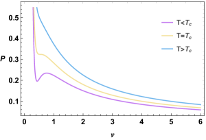
Figure 1: $P-v$ digram of the Hayward-AdS black hole for different values of $T$ by taking $Q=0.1$.

It has been observed from this figure that for the values of the temperature higher to the critical one $T_{C}$, the system behaves like an ideal gas. When the temperature takes the value $T_{C}$, one could talk about the the critical isotherm being characterized by an inflection point corresponding to the critical pressure $P_{C}$ and the critical volume $v_{C}$. The values of the temperature lower to $T_{C}$ represent the unstable thermodynamic region. The critical points should verify the following constraints

$$\frac{\partial P}{\partial\upsilon}=0,\hskip 42.67912pt\frac{\partial^{2}P}{\partial\upsilon^{2}}=0.$$ (3.18)

After computations, we find the critical quantities

$$T_{C} = \frac{\left(5\sqrt{2}-4\sqrt{3}\right)\left(7+3\sqrt{6}\right)^{2/3}}{4\ 2^{5/6}\,\pi\,Q},$$ (3.19)

$$v_{C} = {16}^{1/3}\left(7Q^{3}+{54}^{1/2}Q^{3}\right)^{1/3},$$ (3.20)

$$P_{C} = \frac{3\left(\sqrt{6}+3\right)}{16\ 2^{2/3}\left(3\sqrt{6}+7\right)^{5/3}\pi Q^{2}}.$$ (3.21)

For the reduced moduli space associated with generic charges values, these critical values provide a critical universal ratio

$$\chi_{0}=\frac{P_{C}v_{C}}{T_{C}}=\frac{27-3\sqrt{6}}{50}\simeq 0.393.$$ (3.22)

A this level, one can provide certain comments on such a ratio. First, it is noted that the temperature can be obtained using an alternative way by varying the mass with respect to the entropy. Such a way provides a closed number given by $\frac{2}{5}$. Second, it is observed that this ratio number is different than the one obtained in the charged AdS black holes being $\frac{P_{C}v_{C}}{T_{C}}=3/8$ found also in Van der Waals fluids [3]. Finally, a close examination shows that the function metric of the Hayward-AdS black hole is the relevant responsible of such a distinction.

3.2 Criticality of quintessential solutions

Now we are in position to consider the DE effect on such critical behaviors by introducing a quintessence scalar field. In this regard, the study will be made in terms of two parameters $c$ and $\omega_{q}$ associated with the quintessence intensity and the DE state parameter, respectively. Concretely, we will be interested in how the obtained critical universal number behaves in terms of such a DE field related to the density of quintessence via the relation

$$\rho_{q}=-\frac{c}{2}\frac{3\omega_{q}}{r^{3(\omega_{q}+1)}}.$$ (3.23)

It turns out that one can anticipate a relevant behavior for small values of $c$. To visualize the effect of DE in the critical thermodynamic quantities, we propose the following relation

$$\chi\sim\chi_{0}+\xi_{\omega_{q}}(c,Q).$$ (3.24)

This relation separates the ordinary contributions of the Hayward-AdS black holes and the ones of DE. In fact, $\xi_{\omega_{q}}$ represents the DE contributions. However, $\chi_{0}$ denotes the contribution without DE, given by the Eq (3.22). According to [32], and taking the Einstein equations for static black holes surrounded by the quintessence where the stress-energy tensor involves the additivity and linearity conditions, one finds

$$T^{t}_{t} = T^{r}_{r}=\rho_{q},$$ (3.25)

$$T^{\theta}_{\theta} = T^{\phi}_{\phi}=-\frac{\rho_{q}}{2}(3\omega_{q}+1).$$ (3.26)

In this way, the presence of the quintessence DE field requires that the above metric function $f(r)$ of the Hayward-AdS black hole should be modified as follows

$$f_{\omega_{q}}(r)=1+\frac{r^{2}}{\ell^{2}}-\frac{2Mr^{2}}{r^{3}+Q^{3}}-\frac{c}{r^{3\omega_{q}+1}},$$ (3.27)

where $f_{\omega_{q}}$ is the metric function in the presence of DE. Using Eq.(3.3), we get an exact solution of the Hayward AdS black hole in presence of the quintessential field[60]. As before, the black hole mass $M$ can be obtained by solving the constraint $f_{\omega_{q}}(r)=0$. Precisely, we find

$$M=\frac{\left(Q^{3}+r_{h}^{3}\right)\left((8\,P\,\pi\,+1)r_{h}^{3\omega_{q}+1}-3\,c\right)}{6\,r_{h}^{3\omega_{q}+3}}.$$ (3.28)

It is remarked that the previous mass equation can be recovered by sending $c$ to zero. Exploiting Eq.(3.28) and Eq.(3.13) and using the first law of the black hole thermodynamics, the temperature is found to be

$$T(\omega_{q},c)=\frac{1}{4}\frac{\partial f_{\omega_{q}}}{\partial r}\bigg{|}_{r=r_{h}}=\frac{8\pi Pr_{h}^{5}-2Q^{3}+r_{h}^{3}}{4\pi r_{h}\left(Q^{3}+r_{h}^{3}\right)}-\frac{3r^{-(3\omega_{q}+1)}_{h}\left(Q^{3}(\omega_{q}+1)+r_{h}^{3}\omega_{q}\right)c}{{4\pi r_{h}\left(Q^{3}+r_{h}^{3}\right)}.}.$$ (3.29)

According to the method explored in [3], one can obtain the equation of state for such four-dimensional modified AdS-black hole solutions. For a generic point in the associated moduli space, the computations provide the following state equation

$$P(\omega,c)=\frac{16Q^{3}(\pi Tv+1)+v^{3}(2\pi Tv-1)}{2\pi v^{5}}-\frac{3\times 2^{3\omega_{q}+1}v^{-(3\omega_{q}+1)}\left(8Q^{3}(\omega_{q}+1)+v^{3}\omega_{q}\right)c}{2\pi v^{5}}$$ (3.30)

where $v$ represents the associated specific volume. Taking $c=0$, we recover the ordinary pressure appearing in Eq.(3.16).
Having obtained the relevant thermodynamical quantities, we will be interested in analytical and numerical analysis on the obtained results. Precisely, we discuss the $P-V$ diagram. Motivated by similar activities, we deal with specific values of $\omega_{q}$ and $c$ being extensively studied in connections with the DE contributions. Indeed, the corresponding behaviors are plotted in Fig.(2).

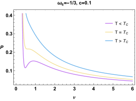
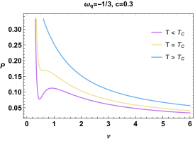
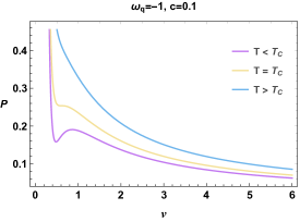
Figure 2: $P-v$ diagram for Hayward-AdS black hole for different values of $T$, $c$, and $\omega_{q}$ by taking $Q=0.1$.

It has been observed that for different values of DE parameters, we find similar behaviors for the $P-v$ diagram appearing in the ordinary Hayward-AdS black hole solutions without DE contributions. However, the one difference is that the unstable thermodynamic region associated with such values of the DE parameter is relevant with respect to the ordinary ones. Taking different values of $\omega_{q}$ and considering $c=0.1$, the critical quantities are almost the same. For $\omega_{q}=-1/3$ and $c=0.3$, however, the critical values are lower with respect to other models. Similar behaviors appear in the ordinary solutions. In the $P-V$ diagram, the inflection points should verify the following constraints

$$\frac{\partial P(\omega,c)}{\partial\upsilon}=0,\hskip 42.67912pt\frac{\partial^{2}P(\omega,c)}{\partial\upsilon^{2}}=0.$$ (3.31)

An examination reveals that the solution of equation (3.31) can be obtained by taking a fixed value of $\omega_{q}$. This will be exploited to get the expression of the critical quantities $T_{c}$, $v_{c}$, and $P_{c}$. Instead of taking generic expressions, we examine only three different $\omega$-models. For $\omega_{q}$=-1, we obtain the following critical quantities

$$T_{C} = \frac{\left(5\sqrt{2}-4\sqrt{3}\right)\left(7+3\sqrt{6}\right)^{2/3}}{4\ 2^{5/6}\,\pi\,Q}$$ (3.32)

$$v_{C} = {16}^{1/3}\left(7Q^{3}+{54}^{1/2}Q^{3}\right)^{1/3}$$ (3.33)

$$P_{C} = \frac{3\left(\sqrt{6}+3\right)}{16\ 2^{2/3}\left(3\sqrt{6}+7\right)^{5/3}\pi Q^{2}}+\frac{c}{8\pi}.$$ (3.34)

In this model, the behavior of the extended universal ratio takes a nice form. Precisely, it can be written

$$\chi_{c}=\chi_{0}+\xi_{-1}(c,Q).$$ (3.35)

After calculations, we find

$$\xi_{-1}(c,Q)=\frac{3\ 2^{2/3}\left(416\sqrt{6}+1019\right)cQ^{2}}{\left(3\sqrt{6}+7\right)^{7/3}}.$$ (3.36)

This is a nice general expression since it gives, as a particular case for $c=0$, the value $\frac{27-3\sqrt{6}}{50}$ for generic charge values. Taking $\omega_{q}=-\frac{2}{3}$, due to the higher degree of the critical parameter equation, we can prove numerically for different values of $Q$ and $c$ that the critical quantities can produce a critical universal number. Indeed, it can be written as

$$\chi_{c}\sim\chi_{0}+\xi_{-\frac{2}{3}}(c,Q).$$ (3.37)

The associated calculations are given in table.(1). For a vanishing value of the $c$ parameter, this can be reduced to the usual value $\chi=\frac{27-3\sqrt{6}}{50}=0.393$ appearing in the black holes without DE contributions given in Eq.(3.22). Taking $\omega_{q}=-\frac{1}{3}$, we get

$$T_{C} = \frac{\left(5\sqrt{2}-4\sqrt{3}\right)\left(7+3\sqrt{6}\right)^{2/3}(1-c)}{4\ 2^{5/6}\,\pi\,Q},$$ (3.38)

$$v_{C} = {16}^{1/3}\left(7Q^{3}+{54}^{1/2}Q^{3}\right)^{1/3},$$ (3.39)

$$P_{C} = \frac{3\left(\sqrt{6}+3\right)(1-c)}{16\ 2^{2/3}\left(3\sqrt{6}+7\right)^{5/3}\pi Q^{2}}.$$ (3.40)

This provides exactly Eq.(3.22). For $c=0$, we can show that the critical thermodynamic quantities are equivalents to the Hayward black hole solutions in EGB gravity by taking the limit $\alpha\to 0$[41]. In this model, the expression of the universal ratio does not depend on the $(Q,c)$ moduli space. It is valid for generic charge values of such quintessential black holes.
To inspect the influence $\omega_{q}$ for generic regions of the $(Q,c)$ moduli space, we should compute the ratio $\frac{P_{C}v_{C}}{T_{C}}$. The calculations are listed in Table.(1).

			$\omega=-1$			$\omega=-\frac{2}{3}$			$\omega=-\frac{1}{3}$
		$c=0$	$c=0.1$	$c=0.2$	$c=0.3$	$c=0.1$	$c=0.2$	$c=0.3$	$c=0.1$	$c=0.2$	$c=0.3$
	$T_{c}$	0.376	0.376	0.376	0.376	0.363	0.350	0.337	0.339	0.301	0.263
	$v_{c}$	0.612	0.612	0.612	0.612	0.608	0.604	0.600	0.612	0.612	0.612
	$P_{c}$	0.241	0.265	0.347	0.277	0.245	0.249	0.252	0.217	0.193	0.169
$Q=0.1$	${\bf\frac{P_{c}v_{c}}{T_{c}}}$	0.393	0.412	0.431	0.451	0.410	0.429	0.449	0.393	0.393	0.393
	$T_{c}$	0.188	0.188	0.188	0.188	0.175	0.162	0.149	0.169	0.150	0.131
	$v_{c}$	1.224	1.224	1.224	1.224	1.209	1.194	1.178	1.224	1.224	1.224
	$P_{c}$	0.060	0.072	0.084	0.096	0.062	0.075	0.088	0.054	0.048	0.042
$Q=0.2$	${\bf\frac{P_{c}v_{c}}{T_{c}}}$	0.393	0.470	0.548	0.625	0.429	0.552	0.693	0.393	0.393	0.393
	$T_{c}$	0.125	0.125	0.125	0.125	0.112	0.099	0.087	0.113	0.100	0.087
	$v_{c}$	1.836	1.836	1.836	1.836	1.802	1.768	1.734	1.836	1.836	1.836
	$P_{c}$	0.026	0.038	0.050	0.062	0.092	0.105	0.117	0.024	0.021	0.018
$Q=0.3$	${\bf\frac{P_{c}v_{c}}{T_{c}}}$	0.393	0.567	0.742	0.916	1.486	1.863	2.336	0.393	0.393	0.393
	$T_{c}$	0.094	0.094	0.094	0.094	0.095	0.081	0.067	0.084	0.075	0.065
	$v_{c}$	2.449	2.449	2.449	2.449	2.147	2.124	2.100	2.449	2.449	2.449
	$P_{c}$	0.015	0.038	0.044	0.050	0.020	0.021	0.022	0.013	0.012	0.010
$Q=0.4$	${\bf\frac{P_{c}v_{c}}{T_{c}}}$	0.393	0.703	1.013	1.324	0.467	0.558	0.688	0.393	0.393	0.393

Table 1: Numerical values of critical thermodynamic parameters in the presence of DE.

It has been observed that the expression of the critical universal ratio has certain nice features. For $\omega_{q}$ models, it depends on the $(Q,c)$ moduli space. Fixing the value of $\omega_{q}$ and considering the line $(Q,0)$ of the reduced moduli space, it reduces to the usual value $\chi_{0}=0.393$. At a generic point of the moduli space, we remark that when $\omega_{q}$ increases, the quantity $\frac{P_{c}\nu_{c}}{T_{c}}$ decreases by approaching the value $\chi_{0}$. Taking $\omega_{q}=-\frac{1}{3}$, in generic regions of the moduli space, it has been observed that this critical ratio is independent of the DE parameter for all range of $c$. This can be understood from the fact that the associated model could correspond to a possible length scaling for $\omega_{q}=-\frac{1}{3}$

$$\frac{1}{\ell^{2}}\to\frac{1}{\ell^{2}}-c.$$ (3.41)

For the ordinary solution and the $\omega_{q}=-\frac{1}{3}$ model, we get the same value of the ratio $\frac{P_{C}\nu_{C}}{T_{C}}$. This critical ratio is closed to the value $\frac{3}{8}$, obtained in AdS black hole solutions [52, 53]. However, for $\omega_{q}=-\frac{2}{3}$ and $\omega_{q}=-1$ models, the ratio $\frac{P_{c}\nu_{c}}{T_{c}}$ increases with $c$ and $Q$. Taking small values of $c$ and $Q$, this ratio increases slightly. This shows that the effect of $c$ is negligible for such models.

4 Heat engine behaviors from quintessence

Considering the Hayward-AdS black holes as heat engines, we compute and investigate the associated efficiency. In particular, we inspect the effect of the quintessence field on such heat engine behaviors. Before going ahead, we note that the heat engine is constructed into a closed path in the $P-V$ plane. It is recalled that the heat absorbed is defined as $Q_{H}$ and the heat discharged is given by $Q_{C}$ as represented in Fig.(3). To go beyond the previous thermodynamical proprieties, we compute the specific heat at constant volume and at constant pressure. In particular, one has

$$C_{V}=T\left(\frac{\partial S}{\partial T}\right)_{V}=0.$$ (4.1)

However, the heat capacity at constant pressure is found to be

$$C_{p}=T\left(\frac{\partial S}{\partial T}\right)_{p}.$$ (4.2)

This quantity is needed to investigate the associated work from the heat energy according to a cycle between two sources (cold/hot) with the temperatures $T_{cold}$ and $T_{hot}$, respectively. Then, we make contact with the Carnot cycle defined as a simple cycle described by two isobars and two isochores as reported in [44]. These configurations are illustrated in Fig.(3). In particular, we examine the DE effect on the efficiency of the Hayward-AdS black holes, as represented in Figure.(3), The heat engine is drown by a rectangular cycle $(1\longrightarrow 2\longrightarrow 3\longrightarrow 4\longrightarrow 1)$ in the $P-V$ plane.

Figure 3: Left: Carnot cycle. Right: The studied cycle.

The output work $W$, being the area of the rectangle, is given by

$$W=\oint PdV=P_{1}\left(V_{2}-V_{1}\right)+P_{4}\left(V_{4}-V_{3}\right).$$ (4.3)

Developing the calculations, one obtains

$$W=\frac{4}{3\sqrt{\pi}}\left({S_{2}}^{\frac{3}{2}}-{S_{1}}^{\frac{3}{2}}\right)\left(P_{1}-P_{4}\right).$$ (4.4)

Since $C_{V}=0$, we should compute the heat $Q_{H}$ during the process $1\longrightarrow 2$. Indeed, the heat $Q_{H}$ can be calculated using the following integral

$$Q_{H}=\int_{T_{1}}^{T_{2}}C_{p}\left(P_{1},T\right)dT=\int_{S_{1}}^{S_{2}}\left(\frac{\partial T}{\partial S}\right)dS=\int_{S_{1}}^{S_{2}}TdS=M_{2}-M_{1}.$$ (4.5)

Using Eq.(3.28), we obtain

$$Q_{H}=\frac{6cS\pi^{\frac{3\omega_{q}}{2}}\left(\pi^{2}Q^{3}(\omega_{q}+1)+\sqrt{\pi}S^{\frac{3}{2}}\omega_{q}\right)+2S^{\frac{3(\omega_{q}+1)}{2}}\left(S^{\frac{3}{2}}(8PS+1)-2\pi^{\frac{3}{2}}Q^{3}\right)}{S^{\frac{3\omega_{q}}{2}}\left(S^{2}(8PS-1)+8\pi^{\frac{3}{2}}Q^{3}\sqrt{S}\right)-3c\pi^{\frac{3\omega_{q}}{2}+\frac{1}{2}}\left(\pi^{\frac{3}{2}}Q^{3}\left(3\omega_{q}^{2}+8\omega_{q}+5\right)+S^{\frac{3}{2}}\omega_{q}(3\omega_{q}+2)\right)}.$$ (4.6)

Dividing the work by this expression, we can get the efficiency. Indeed, it is given by

$$\eta=\frac{W}{Q_{H}}=\frac{8({P_{1}}-P_{4})\left({S_{2}}^{\frac{3}{2}}-{S_{1}}^{\frac{3}{2}}\right)}{\beta_{S1}{S_{1}}^{-\frac{3}{2}(\omega_{q}+1)}\left(3c\pi^{\frac{3\omega_{q}}{2}+\frac{1}{2}}-\alpha_{S1}\right)+\beta_{S2}{S_{2}}^{-\frac{3}{2}(\omega_{q}+1)}\left(\alpha_{S2}-3c\pi^{\frac{3\omega_{q}}{2}+\frac{1}{2}}\right)}$$ (4.7)

where the entropy functions $\alpha_{S}$ and $\beta_{S}$ take the following form

$$\alpha_{S} = (8P_{1}S+3)S^{\frac{3\omega_{q}}{2}+\frac{1}{2}},$$ (4.8)

$$\beta_{S} = \pi^{\frac{3}{2}}Q^{3}+S^{\frac{3}{2}}.$$ (4.9)

Considering $Q=0$, we recover a similar equation of $\eta$ as reported in [44]. A close examination shows that small c expansions provide the following expression

$$\eta\sim\eta(c=0)+\eta(c)+O\left(c^{2}\right),$$ (4.10)

where $\eta(c=0)$ and $\eta(c)$ are giving by

$$\eta(c=0) = \frac{8{S_{1}}{S_{2}}({P_{1}}-{P_{4}})\left({S_{2}}^{\frac{3}{2}}-{S_{1}}^{\frac{3}{2}}\right)}{\beta_{S2}(8{P_{1}}{S_{2}}+3){S_{1}}-\beta_{S1}(8{P_{1}}{S_{1}}+3){S_{2}}},$$ (4.11)

$$\eta(c) = \frac{8c\left((\gamma_{S1}-\gamma_{S2})({P_{1}}-{P_{4}})\left({S_{2}}^{\frac{3}{2}}-{S_{1}}^{\frac{3}{2}}\right)\right)}{\left(\alpha_{S2}\beta_{S2}{S_{2}}^{-\frac{3}{2}(\omega_{q}+1)}-\alpha_{S1}\beta_{S1}{S_{1}}^{-\frac{3}{2}(\omega_{q}+1)}\right)^{2}}$$ (4.12)

and where one has used $\gamma_{S}=3\beta_{S}\pi^{\frac{3\omega_{q}}{2}+\frac{1}{2}}S^{\frac{1}{2}(-3)(\omega_{q}+1)}$. This expression should be compared with the Carnot efficiency $\eta_{car}$ by investigating the ratio $\frac{\eta}{\eta_{car}}$. Indeed, the efficiency of the Carnot engine is given by

$$\eta_{car}=1-\frac{T_{cold}}{T_{hot}}=1-\frac{T\left(P_{4},S_{1}\right)}{T\left(P_{1},S_{2}\right)}.$$ (4.13)

By employing the previous equations, the efficiency $\eta$ can take the following form

$$\eta_{car}=1-\frac{S_{2}^{\frac{1}{2}(3\omega_{q}+1)}\beta_{S2}(\lambda_{S1P4}+c\,\delta_{S1})}{S_{1}^{\frac{1}{2}(3\omega_{q}+1)}\beta_{S1}(\lambda_{S2P1}+c\,\delta_{S2})},$$ (4.14)

where one has

$$\lambda_{SP}=S^{\frac{1}{2}(3\omega_{q}+1)}\left(S^{\frac{3}{2}}(8PS+1)-2\pi^{\frac{3}{2}}Q^{3}\right)$$ (4.15)

and where the entropy function $\delta_{S}$ is given by

$$\delta_{S}=3\pi^{\frac{3\omega_{q}}{2}}\left(\pi^{2}Q^{3}(\omega_{q}+1)+\sqrt{\pi}S^{\frac{3}{2}}\omega_{q}\right).$$ (4.16)

Carrying out small c expansions, the Carnot efficiency $\eta_{car}$ reduces to

$$\eta_{car}\sim\eta_{car}(c=0)+\eta_{car}(c)+O\left(c^{2}\right),$$ (4.17)

where the involved terms are

$$\eta_{car}(c=0) = 1-\frac{S_{2}^{\frac{1}{2}(3\omega_{q}+1)}\beta_{S2}(\lambda_{S1P4}+c\,\delta_{S1})}{S_{1}^{\frac{1}{2}(3\omega_{q}+1)}\beta_{S1}(\lambda_{S2P1}+c\,\delta_{S2})},$$ (4.18)

$$\eta_{car}(c) = -\frac{S_{2}^{\frac{1}{2}(3\omega_{q}+1)}\beta_{S2}(\delta_{S1}\lambda_{S2P1}-\delta_{S2}\lambda_{S1P4})c}{S_{1}^{\frac{1}{2}(3\omega_{q}+1)}\beta_{S1}(\lambda_{S2P1})^{2}}.$$ (4.19)

It follows from these calculations that the heat engine efficiency depends on the involved quantities including the dark energy density, the state parameter, the entropy and the pressure. To visualize clearly the associated behaviors, we consider the variations of the efficiency in terms of various quantities. In particular, we consider three models corresponding to the known values of the state parameter $\omega=-1,-\frac{2}{3},-\frac{1}{3}$.
Concretely, Fig.(4) illustrates the variations of the efficiency $\eta$ and the ratio $\frac{\eta}{\eta_{car}}$ with respect to $S_{2}$ by taking different values of the state parameter.

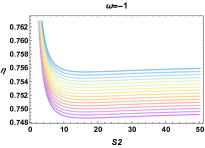
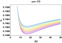
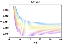
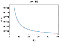
Figure 4: The functional relationship between the thermal engine efficiency $\eta$, the ratio $\eta/\eta_{car}$ and the entropy $S_{2}$ of the Hayward-AdS surrounded by quintessence field for different values of $\omega_{q}$ and $c$. It has been taken $Q=0.3$, $P_{1}=4$, $S_{1}=1$ and $P_{4}=1$.

First, we analyze the variation of the efficiency $\eta$. For $\omega_{q}=-1$ and $\omega_{q}=-\frac{2}{3}$, the efficiency decreases by increasing the entropy $S_{2}$ and by decreasing $c$. Moreover, it is almost constant for large entropy $S_{2}$ for different values of $c$. For $\omega=-\frac{1}{3}$, however, the behavior is quite different. The efficiency of the heat engine decreases for a certain range of the entropy. After reaching specific values, it increases with $S_{2}$. Varying $S_{2}$, the efficiency increases by increasing the DE filed intensity $c$. However, it is observed that the variation $\eta$ as a function of $S_{2}$ presents a minimum, which increases by increasing $c$. However, this minimum is not observed in the $\eta-S_{2}$ plane for the quintessential charged AdS black holes[44]. The variation of $\frac{\eta}{\eta_{car}}$ in terms of $S_{2}$ involves similar properties for the three $\omega$ models. In particular, it decreases by increasing $S_{2}$. For $\omega_{q}=-1$ and $\omega_{q}=-\frac{1}{3}$, we observe that the field intensity $c$ provides a non relevant effect on the ratio $\frac{\eta}{\eta_{car}}$. For $\omega_{q}=-1$, however, the ratio $\frac{\eta}{\eta_{car}}$ increases by increasing the DE filed intensity $c$.
Now, we move to examine the variation of the efficiency in terms of the pressure $P_{1}$ by varying $c$ and $\omega_{q}$. The associated behaviors are illustrated in Fig.(5) by scaling such a parameter as $10c$.

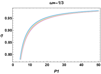
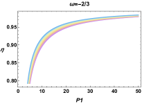
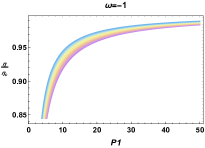
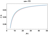
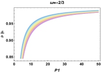
Figure 5: The functional relationship between the thermal engine efficiency $\eta$, the ratio $\eta/\eta_{car}$ and the pressure $P_{1}$ of the Hayward-AdS surrounded by quintessence field for different values of $\omega_{q}$ and $c$. It has been taken $Q=0.1$, $S_{1}=1$, $P_{4}=1$ and $S_{2}=4$.

It has been remarked that $\eta$ and $\frac{\eta}{\eta_{car}}$ involve similar aspects. For the $P_{1}$ variation, all panels obviously reveal that always there is a monotonous trend of an increase. Moreover, the efficiency of the heat engine approaches the maximum possible value $1$ by augmenting the pressure $P_{1}$. Taking $\omega_{q}=-\frac{1}{3}$, the effect of $c$ on the efficiency $\eta$ and the ratio $\frac{\eta}{\eta_{car}}$ is negligible. For $\omega_{q}=-1$ and $\omega_{q}=-\frac{2}{3}$, however, they increase by increasing $c$.
To see the effect of $\omega_{q}$ on such behaviors, we plot in Fig.(6) the variation of such quantities with respect to the entropy $S_{2}$ for three different values of the DE state parameter.

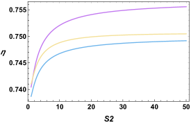
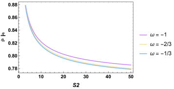
Figure 6: The variation of efficiency $\eta$ and the ratio $\eta/\eta_{car}$ as function of $S_{2}$ for different values of $\omega_{q}$ by taking $c=0.3$, $Q=0.3$, $P_{1}=4$, $S_{1}=1$ and $P_{4}=1$.

From Fig.(6), one can observe that the black hole cycle is more efficient when the parameter $\omega_{q}$ decreases. For the ratio between the efficiency and the Carnot efficiency ($\frac{\eta}{\eta_{car}}$), it has been seen that, for small values of the entropy $S_{2}$, all the efficiencies are the same. When the entropy becomes important with respect the pressure, the $\frac{\eta}{\eta_{car}}$ curves separate. In particular, the ratio $\frac{\eta}{\eta_{car}}$ increases when the parameter $\omega_{q}$ decreases.

5 Optical aspect of quintessential Hayward-AdS black holes

In this section, we investigate the optical properties of the charged quintessential Hayward-AdS black holes. Precisely, we approach the shadow geometrical configurations in terms of the involved parameters.

5.1 Shadow behaviors

Following to the activities associated with such quintessential AdS-black holes [54, 55], the massless particle equations of motion can be obtained by employing the Hamilton-Jacobi method for a photon in the associated spacetime. The associated equation reads as

$$\frac{\partial S}{\partial\tau}=-\frac{1}{2}g^{ij}p_{i}p_{j},$$ (5.1)

where $S$ and $\tau$ are the Jacobi action and the affine parameter respectively, along the geodesics. In the spherically symmetric spacetime, the motion of photon can be controlled by the following Hamiltonian

$$H=\frac{1}{2}g^{ij}p_{i}p_{j}=0.$$ (5.2)

For simplicity reasons, we consider the photon motion on the equatorial plane $\theta=\frac{\pi}{2}$. Indeed, one can get the Hamiltonian equation of the photon given by

$$(rf(r)p_{r})^{2}-r^{2}p_{t}^{2}+f(r)p_{t}^{2}=0$$ (5.3)

where $E=-p_{t}$ and $L=p_{\phi}$ are the conserved total energy and the conserved angular momentum of the photon, respectively. It is recalled that it has been used the $p_{\mu}$ notation being the four-momentum. Using the Hamiltonian-Jacobi formalism, the equations of motion can be formulated as

$$\frac{dt}{d\tau} = \frac{E}{f(r)},$$

$$\frac{dr}{d\tau} = \pm\sqrt{f(r)\left(\frac{E^{2}}{f(r)}-\frac{L^{2}}{r^{2}}\right)},$$

$$\frac{d\phi}{d\tau} = -\frac{L}{r^{2}}.$$ (5.4)

Indeed, the shape of a black hole is totally defined by the limit of its shadow being the visible shape of the unstable circular orbits of the photons. To reach that, one exploits the radial equation of motion. The latter takes the following form

$$\Big{(}\frac{dr}{d\tau}\Big{)}^{2}+V_{eff}(r)=0,$$ (5.5)

where $V_{eff}(r)$ indicates the effective potential for a radial particle motion. In particular, it is given by

$$V_{eff}=f(r)\left(\frac{L^{2}}{r^{2}}-\frac{E^{2}}{f(r)}\right).$$ (5.6)

The maximal value of the effective potential which provides the circular orbits and the unstable photons is required by the following constraint

$$V_{eff}=\frac{dV_{eff}}{dr}\Big{|}_{r=r_{p}}=0.$$ (5.7)

Using Eq.(5.6) and Eq.(5.7), one can obtain

$$V_{eff}|_{r=r_{p}}=\frac{dV_{eff}}{dr}\Big{|}_{r=r_{p}}=\left\{\begin{array}[]{ll}&f(r)\left(\frac{L^{2}}{r_{p}^{2}}-\frac{E^{2}}{f(r_{p})}\right)=0,\\ \\ &L^{2}\left(\frac{r_{p}f^{\prime}(r_{p})-2f(r_{p})}{r_{p}^{3}}\right)=0,\end{array}\right.$$ (5.8)

where one has used the notation $f^{\prime}(r)=\frac{\partial f(r)}{\partial r}$. The photon sphere radius $r_{p}$ of the quintessential Hayward-AdS black holes corresponds to the real and the positive solution of the following constraint

$$r_{p}f^{\prime}(r_{p})-2f(r_{p})=0.$$ (5.9)

It has been remarked that the AdS backgrounds do not affect the photon sphere radius $r_{p}$. It follows from Eq.(5.9) that it is complicated to determine $r_{p}$ analytically. However, we can perform a numerical computation to solve the corresponding equation. The orbit equation for the photon is obtained by considering the equation

$$\frac{dr}{d\phi}=\pm\frac{r^{2}}{L}\sqrt{f(r)\left(\frac{E^{2}}{f(r)}-\frac{L^{2}}{r^{2}}\right)}.$$ (5.10)

It is noted that the photon orbit is constrained by

$$\frac{dr}{d\phi}\Big{|}_{r=R}=0.$$ (5.11)

Then, the previous equation becomes

$$\frac{dr}{d\phi}=\pm r\sqrt{f(r)\left[\frac{r^{2}f(R)}{R^{2}f(r)}-1\right]}.$$ (5.12)

To get the desired equation, we should consider a light ray sending from a static observer situated at $r_{ob}$ and transmitting into the past with an angle $\alpha_{ob}$ with respect to the radial direction. In this way, one has

$$\cot\alpha_{ob}=\frac{\sqrt{g_{rr}}}{\sqrt{g_{\phi\phi}}}\frac{dr}{d\phi}{\Big{|}}_{r=r_{ob}}=\frac{1}{r\sqrt{f(r)}}\frac{dr}{d\phi}{\Big{|}}_{r=r_{ob}}.$$ (5.13)

Exploiting Eq.(5.13), one gets

$$\sin^{2}\alpha_{ob}=\frac{f(r_{ob})R^{2}}{r_{ob}^{2}f(R)}.$$ (5.14)

In this context, one could obtain the angular radius of the black hole shadow by sending $R$ to $r_{p}$ which is the circular orbit radius of the photon appearing in Eq.(5.9). Precisely, the shadow radius of the black hole observed by a static observer placed at $r_{ob}$ has been found to be

$$r_{s}=r_{ob}\sin\alpha_{ob}=\left.R\sqrt{\frac{f(r_{ob})}{f(R)}}\right|_{R=r_{p}}.$$ (5.15)

As the previous sections, taking small values of the DE field intensity, the radius can be factorized as

$$r_{s}\sim r_{s}(c=0)+r_{s}(c)+O\left(c^{2}\right),$$ (5.16)

where the involved terms are given by

$$r_{s}(c=0) = R\sqrt{\frac{g(r_{ob})}{g(R)}}$$ (5.17)

$$r_{s}(c) = \frac{R\left(g(R)g^{\prime}(r_{ob})-g(r_{ob})g^{\prime}(R)\right)c}{2g(R)\sqrt{g(R)g(r_{ob})}}$$ (5.18)

with $g(r)=f(r,c=0)$ and $g^{\prime}=\frac{\partial f}{\partial c}$. Following [56], the apparent shape of the shadow is obtained by using the celestial coordinates $x$ and $y$. They are defined by

$$x = \lim_{r_{0}\longrightarrow\infty}\left(-r_{0}^{2}\sin\theta_{0}\frac{d\phi}{dr}\Big{|}_{(r_{0},\theta_{0})}\right),$$

$$y = \lim_{r_{0}\longrightarrow\infty}\left(r_{0}^{2}\frac{d\theta}{dr}\Big{|}_{(r_{0},\theta_{0})}\right).$$ (5.19)

Fixing the value of the state parameter to $\omega=-\frac{1}{3}$, the shadow geometries are illustrated in Fig.(7).

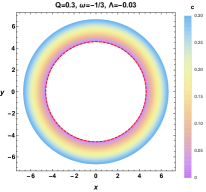
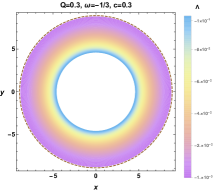
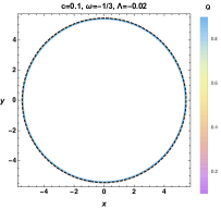
Figure 7: The Hayward-AdS black hole shadows variation as function of $Q$, $\omega_{q}$ and $\Lambda$ in the celestial plane. Dashed and red, brown and black circles correspond to $c=0$, $\Lambda=0$ and $Q=0$, respectively.

For $Q=0.3$ and $\Lambda=-0.03$, it has been remarked that $c$ controls the size of the shadows. It increases with the DE field intensity. It has been observed that the shadows of the ordinary Hayward-AdS black holes involve small radius compared to the quintessential ones[57, 58]. Taking $Q=0.3$ and $c=0.3$, we remark similar behaviors in terms of the cosmological constant. An examination shows that the flat solution involves a large radius compared to the AdS backgrounds. For $c=0.1$ and $\Lambda=-0.02$, however, the charge provides a negligible effect on the circular shadow geometries. To go beyond such an analysis, we illustrate the radius variation in terms of the quintessence field intensity by taking different values of the involved parameters. This is depicted in Fig.(8).

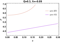
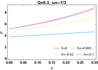
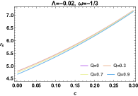
Figure 8: The shadow radius variation as function of $c$ parameter by varying $Q$, $\omega_{q}$ and $\Lambda$ parameters.

For $Q=0.3$ and $\Lambda=-0.09$, it has been observed that the radius of the shadows for $\omega_{q}=-\frac{2}{3}$ are larger than the ones associated with $\omega=-\frac{1}{3}$. This implies that the state parameter could be considered as a parameter controlling the size of the shadow geometries. By increasing the state parameter, the shadow size decreases. Taking $Q=0.3$ and $\omega_{q}=-\frac{1}{3}$, the cosmological constant increases the shadow radius. In the range $0<c<0.15$ with $\omega_{q}=-\frac{1}{3}$ and $\Lambda=-0.02$, the shadow size for $Q=0.09$ is almost smaller with respect to other charge values. In the remaining range, the charge has a negligible effect on the circular shadow behaviors.

5.2 Energy emission rate

Here, we investigate the associated energy emission rate. It is recalled that near the black hole horizons the quantum fluctuations can create and annihilate certain pairs particles. In this regard, the positive energy particles can escape through tunneling from the black hole, inside region where the Hawking radiation occurs. This phenomenon is known as the Hawking radiation which causes the black hole to evaporate in a certain period of time. In what follows, we discuss the corresponding energy emission rate. For a far distant observer, the high energy absorption cross section could approach to the shadow of the black hole. At very high energy, it has been noted that the absorption cross section of the black hole can oscillate to a limiting constant value $\sigma_{lim}=\pi r_{s}^{2}$. Roughly, the energy emission rate can be written as

$$\frac{d^{2}E(\varpi)}{d\varpi dt}=\frac{2\pi^{3}r_{s}^{2}\varpi^{3}}{e^{\frac{\varpi}{T_{{H}}}}-1},$$ (5.20)

where $\varpi$ represents the emission frequency [59], and where $T_{H}$ is the associated Hawking temperature. For the studied model, one takes the temperature given in Eq.(3.29). The energy emission rate is represented in Fig.(9) as a function of $\varpi$ by varying $c$, $\Lambda$ and $Q$ parameters.

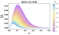
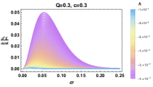
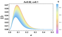
Figure 9: Energy emission rate for different values of DE the intensity $c$, cosmological constant $\Lambda$ and charge $Q$, by takin $\omega_{q}=-1/3$.

It is follows from Fig.(9) that, when DE is present, the energy emission rate is lower. This indicates that the black hole evaporation process is slow. Moreover, we get an even slower radiation process by increasing (decreasing) the intensity $c$ and the charge $Q$ (the cosmological constant $\Lambda$ parameter and the parameter $\omega_{q}$). It has been remarked that the emission rate of the Hayward-AdS black holes is slow compared to other back hole solutions [61, 62, 63].

6 Conclusions and discussions

In this paper, we have investigated the thermodynamic and the optical behaviors of the quintessential Hayward-AdS black holes in four dimensions. For the thermodynamic aspect, we have first reconsidered the study of the critical behaviors of the ordinary black hole solutions. Concretely, we have found that the equation of state provides a universal ratio given by $\chi_{0}=\frac{P_{c}v_{c}}{T_{c}}=\frac{27-3\sqrt{6}}{50}$. For certain values of the DE state parameter $\omega_{q}$, this new number has been modified by a contribution $\xi_{\omega_{q}}(c,Q)$ depending on the DE field intensity and the charge. Then, we have studied the DE effect on the heat engine behaviors of such Hayward AdS black hole solutions by taking certain known values of $\omega_{q}=-1,-\frac{2}{3},-\frac{1}{3}$. For the optical aspect, we have inspected the influence of DE by considering shadow geometries using one dimensional real space. Concretely, we have obtained that the associated radius has been changed by DE contributions. For different values of $\omega_{q}$ the efficiency and the ratio $\eta/\eta_{car}$ go to $1$ by increasing the normalization factor of the quintessence $c$. This can be confirmed by the fact that the quintessence field cools the black hole making it more efficient. Then, we have shown that the Hayward-AdS black holes involve small radius compared to the quintessential ones, in connection with EHT, such new behaviors could take good places. However, the variation of the black hole shadow radius as a function of the parameter $Q$ related to the total magnetic charge $q_{m}$ is neglected. This could reveal that the parameter $Q$ does not affect the black hole shadows.
This work comes with some open questions. A natural question may concern the implementation of other quantities including the rotation parameter. It could be possible to get certain conditions for dark energy models which could be considered as an alternative cosmological model to $\Lambda$CMD. Higher dimensional models could be an interesting investigation in future works.

References

- [1] D. Kastor, S. Ray and J. Traschen, Enthalpy and the Mechanics of AdS Black Holes, Class. Quant. Grav. 26 (2009) 195011, arXiv:0904.2765.
- [2] B. P. Dolan, Pressure and volume in the first law of black hole thermodynamics, Class. Quant. Grav. 28 (2011) 235017, arXiv:1106.6260.
- [3] D. Kubiznak and R. B. Mann, P-V criticality of charged AdS black holes, JHEP 07 (2012) 033, arXiv:1205.0559.
- [4] N. Altamirano, D. Kubiznak and R. B. Mann, Reentrant phase transitions in rotating anti–de Sitter black holes, Phys. Rev. D 88 10 (2013) 101502, arXiv:1306.5756.
- [5] A. Awad, G. G.L. Nashed, Generalized teleparallel cosmology and initial singularity crossing,J.C.A.P 02(2017) 046, arXiv:1701.06899.
- [6] T. Shirafuji, G. G. L. Nashed, Energy and Momentum in the Tetrad Theory of Gravitation , P. T. Phys, 6 (1997) 98, arXiv:gr-qc/9711010.
- [7] E. Elizalde, G.G.L. Nashed, S. Nojiri, S.D. Odintsov, Spherically symmetric black holes with electric and magnetic charge in extended gravity: Physical properties, causal structure, and stability analysis in Einstein’s and Jordan’s frames, Eur. Phys. J. C 2, (2020) 80, arXiv:2001.11357.
- [8] A. Awad, W. El Hanafy, G.G.L. Nashed, S.D.Odintsov, V.K. Oikonomou, Constant-roll Inflation in Teleparallel Gravity, J. C. A. P, 07 (2018)26, arXiv: 1710.00682.
- [9] G. G. L. Nashed, Brane World black holes in Teleparallel Theory Equivalent to General Relativity and their Killing vectors, Energy, Momentum and Angular-Momentum, Chinese Phys. B 19 (2010) 020401, arXiv:0910.5124.
- [10] W. El Hanafy and G. G. L. Nashed, Exact Teleparallel Gravity of Binary Black Holes, Astrophys Space Sci 361,(2016) 68, arXiv:1507.07377.
- [11] G. G.L. Nashed, Schwarzschild solution in extended teleparallel gravity,E.P.L, 105, 10001, arXiv:1501.00974
- [12] D. Kubiznak and F. Simovic, Thermodynamics of horizons: de Sitter black holes and reentrant phase transitions, Class. Quant. Grav. 33 24 (2016) 245001, arXiv:1507.08630.
- [13] N. Altamirano, D. Kubizňák, R. B. Mann and Z. Sherkatghanad, Kerr-AdS analogue of triple point and solid/liquid/gas phase transition, Class. Quant. Grav. 31 (2014) 042001, arXiv:1308.2672.
- [14] R. A. Hennigar, R. B. Mann and E. Tjoa, Superfluid Black Holes, Phys. Rev. Lett. 118 2 (2017) 021301, arXiv:1609.02564.
- [15] K. A. Bronnikov, Regular magnetic black holes and monopoles from nonlinear electrodynamics, Phys. Rev. D 63 (2001) 044005, arXiv:gr-qc/0006014.
- [16] I. Dymnikova, Regular electrically charged structures in nonlinear electrodynamics coupled to general relativity, Class. Quant. Grav. 21 (2004) 4417, arXiv:gr-qc/0407072.
- [17] J. Polchinski, Decoupling Versus Excluded Volume or Return of the Giant Wormholes, Nucl. Phys. B 325 (1989) 619.
- [18] S. A. Hayward, Formation and Evaporation of Regular Black Holes, Phys. Rev. Lett. 96 (2006) 031103, arXiv:gr-qc/0506126.
- [19] V. P. Frolov, M. A. Markov and V. F. Mukhanov, Through a Black Hole Into a New Univers?, Phys. Lett. B 216 (1989) 272.
- [20] V. F. Mukhanov and R. H. Brandenberger, A Nonsingular Universe, Phys. Rev. Lett. 68, (1992)1969.
- [21] V. P. Frolov, Notes on nonsingular models of black holes, Phys. Rev. D 94 10 (2016) 104056, arXiv:1609.01758.
- [22] L. Modesto, Black hole interior from loop quantum gravity, Adv. High Energy Phys. 2008 (2008) 459290, arXiv:gr-qc/0611043.
- [23] G. Bertone and D. Hooper, History of dark matter, Rev. Mod. Phys. 90, 4 (2018) 045002, arXiv:1605.04909.
- [24] D. Huterer and D. L. Shafer, Dark energy two decades after: Observables, probes, consistency tests, Rept. Prog. Phys. 811 (2018) 016901,arXiv:1709.01091.
- [25] R. Gannouji, A Primer on Modified Gravity, Int. J. Mod. Phys. D 28 05 (2019) 1942004.
- [26] A. Belhaj, A. El Balali, W. El Hadri, H. El Moumni, M. B. Sedra, Dark energy effects on charged and rotating black holes, Eur. Phys. J. Plus 134(9) (2019) 422.
- [27] R. R. Caldwell, R. Dave and P. J. Steinhardt, Cosmological imprint of an energy component with general equation of state, Phys. Rev. Lett. 80, (1998) 1582, arXiv:astro-ph/9708069.
- [28] R. Uniyal, N. Chandrachani Devi, H. Nandan and K. D. Purohit, Geodesic Motion in Schwarzschild Spacetime Surrounded by Quintessence, Gen. Rel. Grav. 47 2 (2015) 16, arXiv:1406.3931.
- [29] R. A. Konoplya, Shadow of a black hole surrounded by dark matter, Phys. Lett. B 795, (2019) 6, arXiv:1905.00064.
- [30] N. A. Bahcall, J. P. Ostriker, S. Perlmutter and P. J. Steinhardt, The Cosmic triangle: Assessing the state of the universe, Science 284 (1999) 1481, arXiv:astro-ph/9906463.
- [31] V. Sahni and A. A. Starobinsky, The Case for a positive cosmological Lambda term, Int. J. Mod. Phys. D 9 (2000) 373, arXiv:astro-ph/9904398.
- [32] V. V. Kiselev, Quintessence and black holes, Class. Quant. Grav. 20, (2003) 1187, arXiv:gr-qc/0210040.
- [33] S. Chen, B. Wang and R. Su, Hawking radiation in a -dimensional static spherically-symmetric black Hole surrounded by quintessence, Phys. Rev. D 77, (2008) 124011, arXiv:0801.2053.
- [34] S. Chen, Q. Pan and J. Jing,Holographic superconductors in quintessence AdS black hole spacetime, Class. Quant. Grav. 30 (2013) 145001, arXiv:1206.2069.
- [35] M. Chabab, H. El Moumni, S. Iraoui, K. Masmar and S. Zhizeh, More Insight into Microscopic Properties of RN-AdS Black Hole Surrounded by Quintessence via an Alternative Extended Phase Space,Int. J. Geom. Meth. Mod. Phys. 15, 10 (2018) 1850171, arXiv:1704.07720.
- [36] A. Belhaj, M. Benali, A. El Balali, H. El Moumni and S. E. Ennadifi, Deflection angle and shadow behaviors of quintessential black holes in arbitrary dimensions, Class. Quant. Grav. 37 21 (2020) 215004, arXiv:2006.01078.
- [37] Ö. Ökcü and E. Aydıner, Joule–Thomson expansion of the charged AdS black holes, Eur. Phys. J. C 77 (2017) no.1, 24 [arXiv:1611.06327 [gr-qc]].
- [38] M. Chabab, H. El Moumni, S. Iraoui, K. Masmar and S. Zhizeh, Joule-Thomson Expansion of RN-AdS Black Holes in gravity, LHEP 02 (2018), 05 [arXiv:1804.10042 [gr-qc]].
- [39] A. Belhaj, M. Chabab, H. El Moumni, K. Masmar, M. B. Sedra and A. Segui, On Heat Properties of AdS Black Holes in Higher Dimensions, JHEP 05 (2015), 149 [arXiv:1503.07308 [hep-th]].
- [40] C. V. Johnson, Holographic Heat Engines, Class. Quant. Grav. 31 (2014) 205002, arXiv:1404.5982.
- [41] M. Zhang, C. M. Zhang, D. C. Zou and R. H. Yue, criticality and Joule-Thomson Expansion of Hayward-AdS black holes in 4D Einstein-Gauss-Bonnet gravity, arXiv:2102.04308.
- [42] H. El Moumni and K. Masmar, Regular AdS black holes holographic heat engines in a benchmarking scheme, Nucl. Phys. B 973 (2021), 115590.
- [43] Y-L. Huang and S. Guo, Thermodynamic of the charged accelerating AdS black hole: P-V critical and Joule-Thomson expansion, arXiv:2009.09401 .
- [44] H. Liu and X. H. Meng, Effects of dark energy on the efficiency of charged AdS black holes as heat engines, Eur. Phys. J. C 77 8 (2017) 556, arXiv:1704.04363.
- [45] X. X. Zeng and H. Q. Zhang, Influence of quintessence dark energy on the shadow of black hole, Eur. Phys. J. C 80 (2020) no.11, 1058, arXiv:2007.06333 [gr-qc].
- [46] S. U. Khan and J. Ren, Shadow cast by a rotating charged black hole in quintessential dark energy, Phys. Dark Univ. 30 (2020) 100644,arXiv:2006.11289 [gr-qc].
- [47] O. Pedraza, L. A. López, R. Arceo and I. Cabrera-Munguia, Geodesics of Hayward black hole surrounded by quintessence, Gen. Rel. Grav. 53 (2021) 24, arXiv:2008.00061 [gr-qc].
- [48] A. Abdujabbarov, B. Toshmatov, Z. Stuchlík and B. Ahmedov, Shadow of the rotating black hole with quintessential energy in the presence of plasma, Int. J. Mod. Phys. D 26 (2016) 1750051, arXiv:1512.05206 [gr-qc].
- [49] A. Abdujabbarov, M. Amir, B. Ahmedov and S. G. Ghosh, Shadow of rotating regular black holes, Phys. Rev. D 93 (2016) 104004, arXiv:1604.03809 [gr-qc].
- [50] Z. Y. Fan and X. Wang, Construction of Regular Black Holes in General Relativity, Phys. Rev. D 94 12 (2016) 124027, arXiv:1610.02636.
- [51] Z. Y. Fan, Critical phenomena of regular black holes in anti-de Sitter space-time, Eur. Phys. J. C 77 (2017) no.4, 266, arXiv:1609.04489 [hep-th].
- [52] D. Kubiznak and R. B. Mann, P-V criticality of charged AdS black holes, JHEP 07 (2012) 033, arXiv:1205.0559 [hep-th].
- [53] A. Belhaj, M. Chabab, H. El Moumni and M. B. Sedra, On Thermodynamics of AdS Black Holes in Arbitrary Dimensions, Chin. Phys. Lett. 29 (2012) 100401, arXiv:1210.4617 [hep-th].
- [54] B. Carter, Global structure of the Kerr family of gravitational fields, Phys. Rev. 174 (1968), 1559-1571
- [55] S. Chandrasekhar, The Mathematical Theory of Black Holes, (Oxford University Press, 1998).
- [56] E. F. Eiroa and C. M. Sendra, Shadow cast by rotating braneworld black holes with a cosmological constant, Eur. Phys. J. C 78 (2018) 91, arXiv:1711.08380 [gr-qc].
- [57] A. Belhaj, A. El Balali, W. El Hadri, M. A. Essebani, M. B. Sedra and A. Segui, KerrAdS Black Hole Behaviors from Dark Energy, Int. Jour. of Mod. Phys. D29 (09) (2020) 2050069.
- [58] A. Belhaj, A. El Balali, W. El Hadri, Y. Hassouni, E. Torrente-Lujan, Phase transition and shadow behaviors of quintessential black holes in M-theory/superstring inspired models, Int.J.Mod.Phys. A 36 (2021) 2150057.
- [59] S. W. Wei and Y. X. Liu, Observing the shadow of Einstein-Maxwell-Dilaton-Axion black hole, JCAP 11 (2013) 063, arXiv:1311.4251 [gr-qc].
- [60] Z-Y. Fan and X. Wang, Construction of Regular Black Holes in General Relativity, Phys. Rev. D 94, 124027 (2016), arXiv:1610.02636 [gr-qc].
- [61] A. Belhaj, M. Benali, A. El Balali, W. El Hadri, H. El Moumni, Shadows of Charged and Rotating Black Holes with a Cosmological Constant, Gen. Rel. and Qua. Cos. (2020), arXiv:2007.09058"[gr-qc].
- [62] S. W. Wei, Y. X. Liu, Observing the shadow of Einstein-Maxwell-Dilaton-Axion black hole, JCAP 11 (2013)063, arXiv:1311.4251 [gr-qc].
- [63] S. V. M. C. B. Xavier, Pedro V. P. Cunha, Luıs C. B. Crispino, Carlos A. R. Herdeiro, Shadows of charged rotating black holes: Kerr-Newman versus Kerr-Sen, arXiv:2003.14349.