Natural Image Stitching Using Depth Maps

Abstract

Natural image stitching (NIS) aims to create one natural-looking mosaic from two overlapping images that capture a same 3D scene from different viewing positions. Challenges inevitably arise when the scene is non-planar and the camera baseline is wide, since parallax becomes not negligible in such cases. In this paper, we propose a novel NIS method using depth maps, which generates natural-looking mosaics against parallax in both overlapping and non-overlapping regions. Firstly, we construct a robust fitting method to filter out the outliers in feature matches and estimate the epipolar geometry between input images. Then, we draw a triangulation of the target image and estimate multiple local homographies, one per triangle, based on the locations of their vertices, the rectified depth values and the epipolar geometry. Finally, the warping image is rendered by the backward mapping of piece-wise homographies. Panorama is then produced via average blending and image inpainting. Experimental results demonstrate that the proposed method not only provides accurate alignment in the overlapping regions, but also virtual naturalness in the non-overlapping region.

I Introduction

Natural image stitching (NIS) is a well-studied problem in image processing and computer vision, which composites multiple overlapping images captured from different viewing positions into one natural-looking panorama [27]. The fundamental NIS problem is $2$-into-$1$: given two input images, one reference and one target, to generate one output image that is virtually captured in the reference viewing position, which includes both overlapping and non-overlapping contents as natural as possible. Hence, the first crucial task in NIS is how to warp the target image into an extended view of the reference image, such that the warping result is not only content-consistent in the overlapping region but also view-consistent in the non-overlapping region.

When the capturing scene is planar or the viewing point is stationary, homography is effective for accomplishing the dual task [10]. However, when the 3D scene consists of background objects with non-planar surfaces or even foreground objects with discontinuous depths, meanwhile the baseline is wide, homography cannot generate a natural-looking mosaic because it is not flexible enough to describe the underlying 3D geometry between parallax views (see Fig. 1(b)).

Lots of adaptive warping models are devoted to addressing the parallax issue in NIS. Suppose a set of feature matches between two input images are given, some methods divide the target image into adjacent patches (pixels [7], superpixels [16], rectangles [31], triangles [17], irregular domains [34]) and warp each of them by a local homography using weighted matches; some methods divide the target into rectangular cells and deform them simultaneously via an energy minimization using local (similar [32] or affine [33]) plus global (similar [4] or linearized projective [20]) geometric invariants. Other NIS methods devote attention to combining weighted matches and geometric invariants [2, 21, 18], increasing densities of feature matches [19, 23], pursuing local alignment allowing seamless composition [8, 22]. Nevertheless, existing adaptive warping models are still not fine enough to describe the underlying geometry between large-parallax views such that they still create misaligned or non-natural-looking mosaics at times (see Fig. 1(c-e)).

It is well-known that depth maps are powerful for representing the 3D geometry of a stereo scene and deep learning enables extracting the dense depth map from a single target image [9]. Intuitively, depth maps help align non-matching region or even non-overlapping region (see Fig. 1(f)).

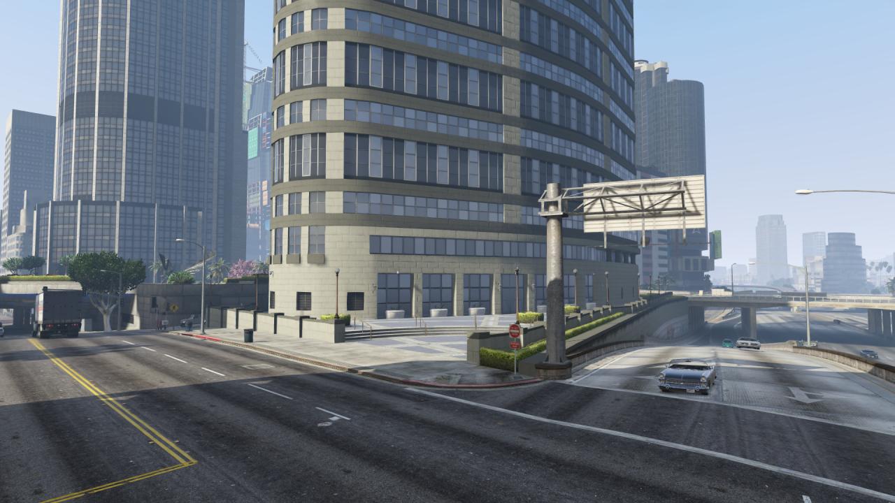
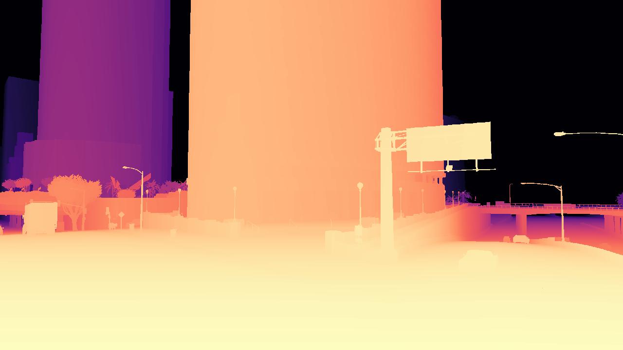
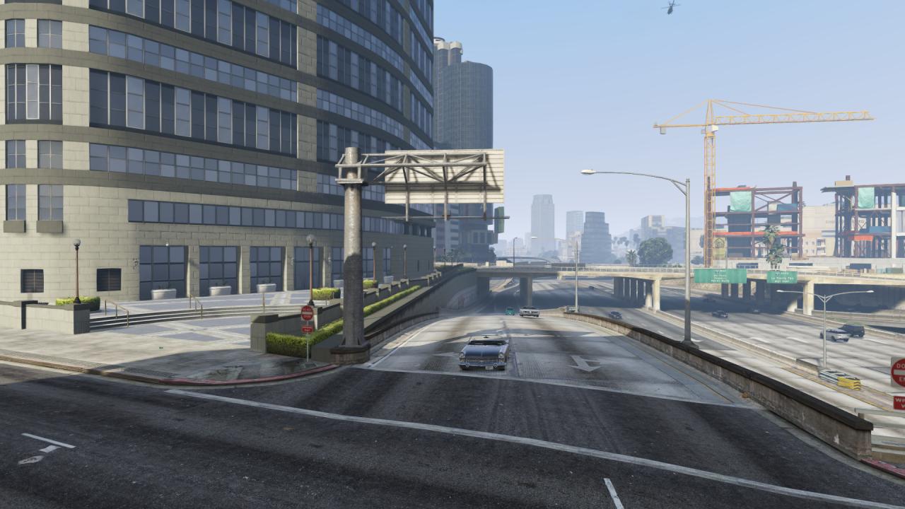
(a) Target image (left), reference image (right) and depth map of the target (middle)

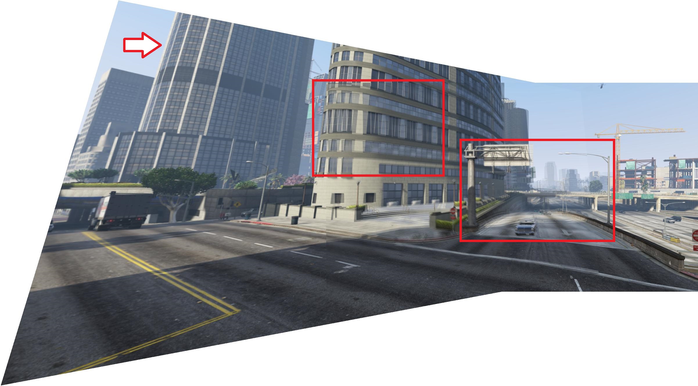
(b) Homography

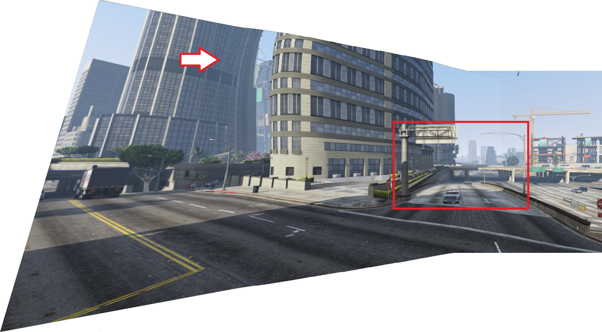
(c) APAP [31]

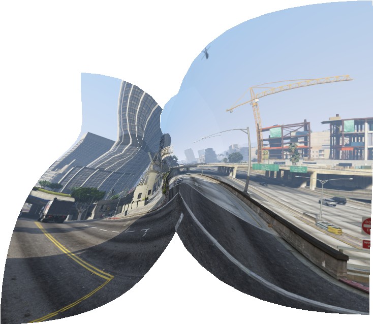
(d) NISwGSP [4]

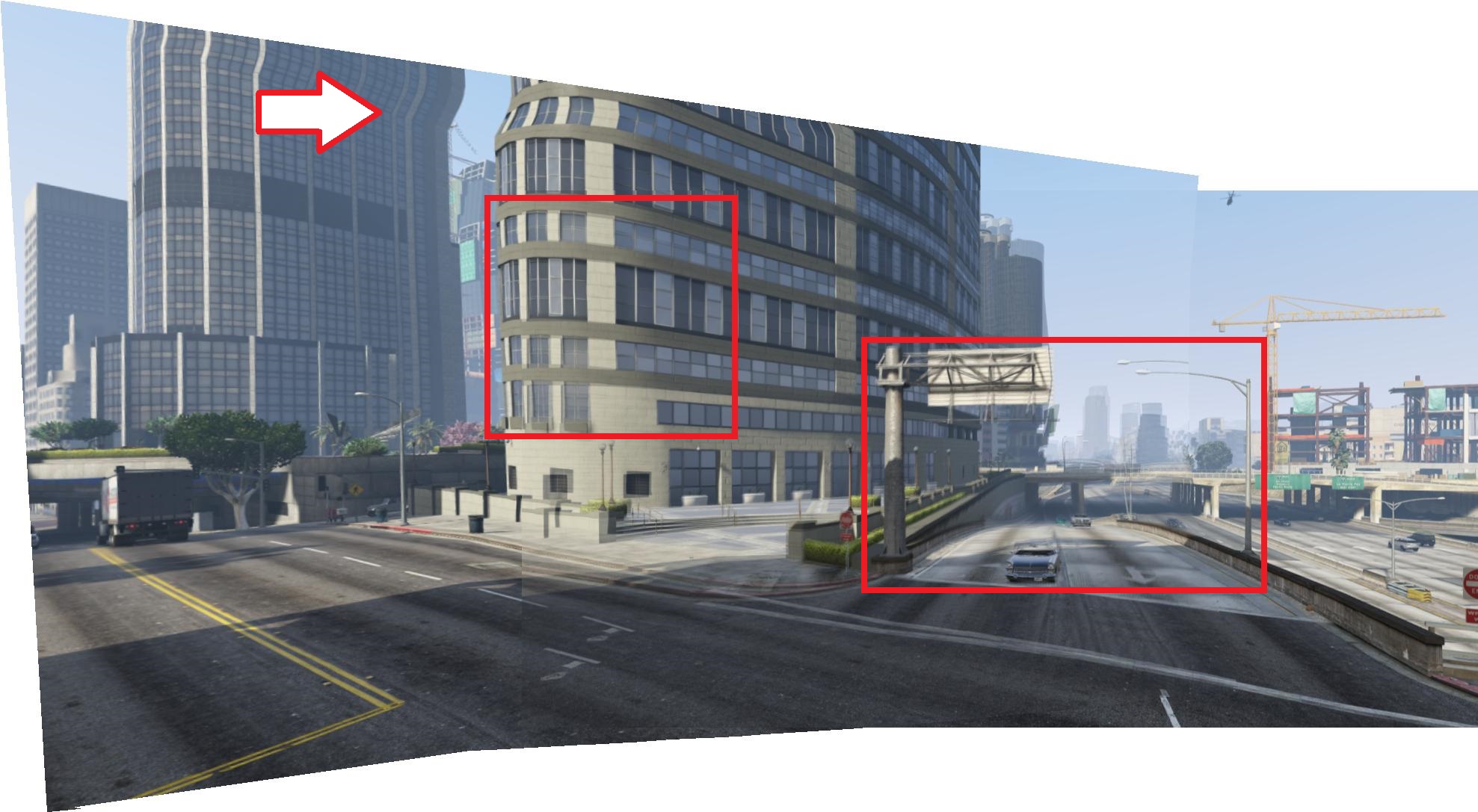
(e) LFA [17]

(f) Warped target image via our method

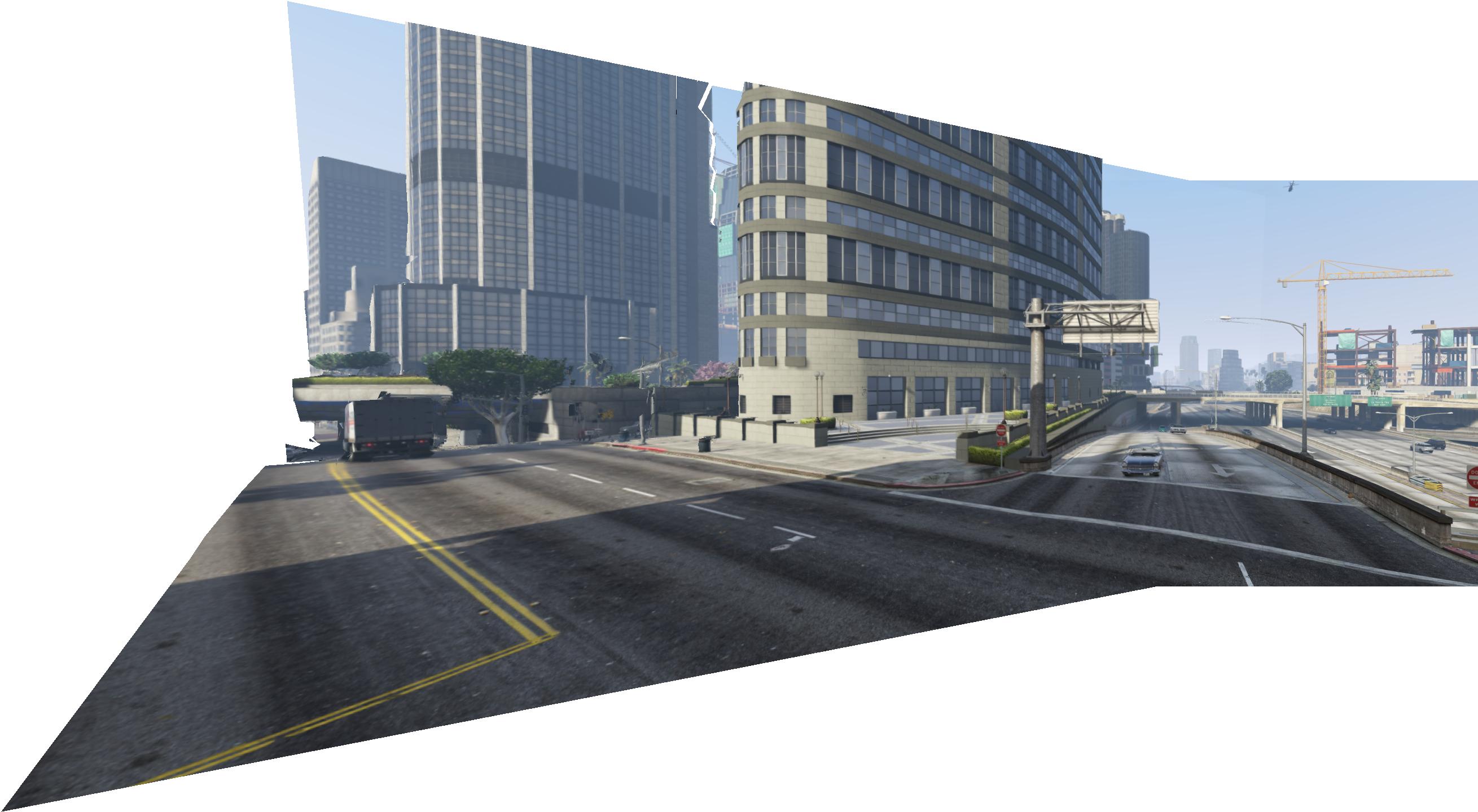
(g) Our final result

Figure 1: Stitching results of 0118 test case from MVS-Synth Dataset [11] via various methods. All results are generated via simple average blending, except that (f) is the rendered target image via our method (best view in color and zoom in).

In this paper, we propose a new NIS method using depth maps against large parallax in both the overlapping and non-overlapping regions. Suppose a set of feature point matches between input images and a depth map of the target image are given, firstly we construct a robust fitting method to filter out the outliers in feature matches and estimate the epipolar geometry of input images; then we draw a triangulation of the target image such that every triangle domain is coplanar in the 3D space; local homographies are estimated, one per triangle, based on locations of its vertices, the rectified depth values and the epipolar geometry; further, the warping image is generated by backward mapping piece-wise homographies; finally, the panorama is produced via average blending and image inpainting. Experimental results show that the stitching mosaics by the proposed NIS method are not only accurately aligned in the overlapping regions but also virtually natural-looking in the non-overlapping regions (see Fig. 1(g)).

The contributions of our work are as follows:

• We propose a robust fitting method to filter out the outliers in feature matches and estimate the epipolar geometry, which is robust to the issue of large parallax;

• We propose a piece-wise homograhies estimation method based on locations of triangle vertices, their rectified depth values and the epipolar geometry, which enables warping the target image discontinuously and naturally to align with the reference image;

The rest of the paper is organized as follows. Section II reviews the related works of adaptive NIS and view synthesis. Section III proposes the novel NIS method using depth maps. Section IV describes the implementation details. Section V presents the experimental results. Section VI concludes the paper.

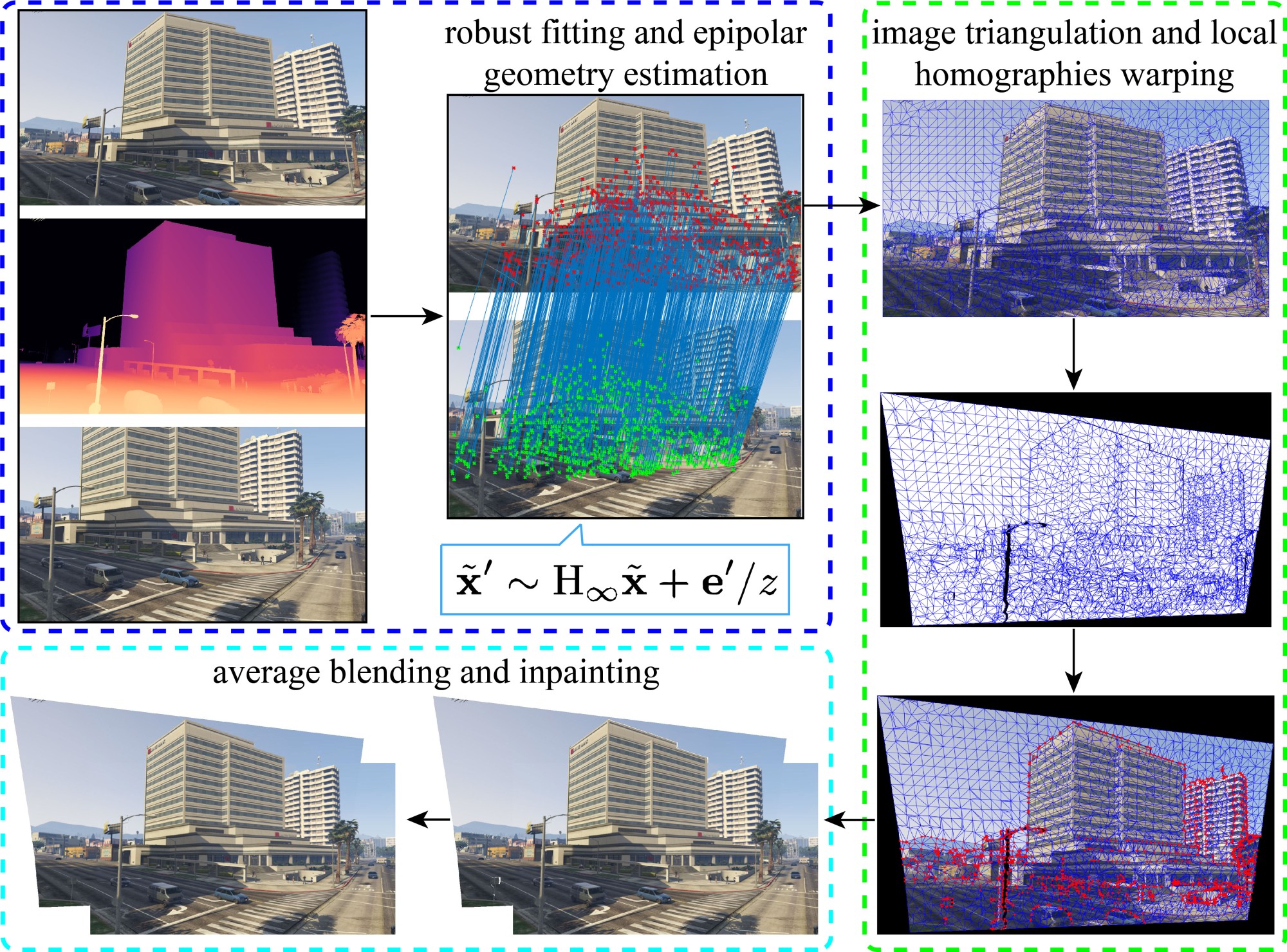
Figure 2: The pipeline of our proposed method, which includes 3 main stages: feature matching and robust fitting (blue box), image triangulation and local warping (green box), image blending and inpainting (cyan box). Stage 1: Point feature matches between input images are extracted, our robust fitting method is then used to filter out the outliers and estimate the epipolar geometry; Stage 2: Delaunay triangulation is applied to the target image, and for each triangle we estimate a local homography warp based on the locations of vertices, its rectified depth values and the epipolar geometry. Then the warped image is rendered via backward texture mapping. Stage 3: Warped images are composited via average blending to generate panorama, in which missing parts are completed via image inpainting.

II Related Work

II-A NIS using weighted matches

Suppose a set of feature matches between two input images is given, some NIS methods adopted piece-wise homographies as adaptive warping models where every local homography is determined via some weighting methods. Gao et al. proposed a dual-homography warping model, where two representative homographies (distant plane $+$ ground plane) are first clustered then the local homography per pixel is estimated by a weighted sum of them [7]. Zheng et al. modified a multiple-homography warping model, where multiple projective-consistent homographies are first clustered and one non-overlapping homography is averaged, then the local homography per pixel is determined by a weighted sum of them [34]. Zaragoza et al. proposed a new as-projective-as-possible (APAP) warp, where the target image is first divided into regular grid cells and the local homography per cell is estimated by moving DLT that assigns more weights to feature matches that located closer to the target cell [31]. Joo et al. appended line matches into the framework of APAP [14]. Recently, Lee and Sim proposed a modified version of APAP, where the target image is divided into superpixels instead of cells and the local homography per superpixel is estimated by moving DLT which assigns more weights to feature points that located on more similar planar regions to the target superpixel instead of explicitly depending on the spatial locations [16]. The most notable advantage of [16] is that it enables a discontinuous warping model against large parallax in the overlapping region. Besides, Li et al. proposed a weighting-free version of APAP, where the target image is divided into adjacent triangle regions whose vertices are either matching feature points or boundary points, then the local homography per triangle is estimated by its vertex matches associated with the relative position between two input views [17]. The advantage of triangulation is apparent as triangles are easier to fulfill coplanar assumption than other patches. However, [17] did not allow vertex split such that large parallax can not be handled. On the contrary, the proposed method uses depth maps to enable triangulation vertex split to handle large parallax not only in the overlapping but also in the non-overlapping regions.

II-B NIS using geometric invariants

Instead of using weighted matches to warping non-matching patches, some NIS methods divide the target image into cells then warp them simultaneously by a deformation, where every mesh is penalized to undergo some geometric invariants (local $+$ global) as much as possible. Zhang and Liu proposed a mesh deformation that uses similar as local geometric invariant and projective as global geometric invariant [32]. Chen and Chuang used similar as both local and global geometric invariants [4]. The estimations of global similarity were comprehensively studied in [2, 21]. In order to address the NIS problem for wide-baseline images, Zhang et al. proposed a mesh deformation that uses affine as local geometric invariant and horizontal-perpendicular-preserving as global geometric invariant [33]. In order to generate perspective-consistent mosaics, Liao and Li used linearized projective [18] as both local and global geometric invariants [20]. Recently, Jia et al. proposed a new local coplanar invariant and a new global collinear invariant [13]. Note that local and global geometric invariants play the roles of interpolation and extrapolation regularizers in the overlapping and non-overlapping regions respectively, while the depth map of the target image can provide more accurate regularizers.

II-C View synthesis using depth maps

Generally speaking, view synthesis (view interpolation) [3] is the task of generating new views of a 3D scene from source views of the scene, where depth maps are commonly adopted to describe the 3D scene from source viewing positions. There are different methods to extract depth maps of source images. Penner and Zhang used depth estimation from multiple images to accomplish novel view synthesis [25]. Wiles et al. leveraged single-image depth predictions implicitly to enable end-to-end view synthesis [30]. In fact, image warping in NIS can also be interpreted as extended view synthesis, taking the target image as the source image and the reference view as the virtual view. However, this paper focuses on using depth maps to improve both alignment and naturalness for NIS rather than appearance modeling [35] and occlusion inpainting in view synthesis tasks [26].

III Proposed Method

In this section, we propose our NIS method using depth maps. The pipeline of our method is illustrated in Fig. 2.

Notations: let the upper-case letters such as $\mathrm{K},\mathrm{R},\mathrm{H}$ denote real matrices, the lower-case letters such as $x,y,z$ denote real values, the bold-faced letters such as $\mathbf{x},\mathbf{e}^{\prime}$ denote real vectors; the symbol $\tilde{\mathbf{x}}$ denotes the homogeneous representation of $\mathbf{x}$, the symbol $[\mathbf{e}^{\prime}]_{\times}$ denotes the skew-symmetric matrix formulated by $\mathbf{e}^{\prime}$.

III-A Robust fitting and epipolar geometry estimation

Given a target image $I_{\mathrm{t}}$ and a reference image $I_{\mathrm{r}}$, suppose their camera matrices are:

$$\mathrm{P}=\mathrm{K}[\mathrm{I}\,|\,\mathbf{0}],\quad\mathrm{P}^{\prime}=\mathrm{K}^{\prime}[\mathrm{R}\,|\,\mathbf{t}],$$ (1)

where $\mathrm{K}\in\mathbb{R}^{3\times 3}$ and $\mathrm{K}^{\prime}\in\mathbb{R}^{3\times 3}$ are two calibration matrices, $\mathrm{R}\in\mathrm{SO}(3)$ is a rotation and $\mathbf{t}\in\mathbb{R}^{3}$ is a translation.

Let $\mathbf{X}\in\mathbb{R}^{3}$ be a world point, $\mathbf{x}\in\mathbb{R}^{2}$ and $\mathbf{x}^{\prime}\in\mathbb{R}^{2}$ be its image points in $I_{\mathrm{t}}$ and $I_{\mathrm{r}}$, and $z\in\mathbb{R}$ be its depth value measured from $\mathrm{P}$, then

$$\tilde{\mathbf{x}}=\mathrm{K}\mathbf{X}/z.$$ (2)

Since $\mathrm{K}$ is invertible, by plugging $\mathbf{X}=z\mathrm{K}^{-1}\tilde{\mathbf{x}}$ into

$$\tilde{\mathbf{x}}^{\prime}\sim\mathrm{K}^{\prime}\mathrm{R}\mathbf{X}+\mathrm{K}^{\prime}\mathbf{t},$$ (3)

where $\sim$ denotes equality up to scale, we obtain

$$\tilde{\mathbf{x}}^{\prime}\sim\mathrm{K}^{\prime}\mathrm{R}\mathrm{K}^{-1}\tilde{\mathbf{x}}+\mathrm{K}^{\prime}\mathbf{t}/z.$$ (4)

Let $\mathrm{H}_{\infty}=\mathrm{K}^{\prime}\mathrm{R}\mathrm{K}^{-1}$ and $\mathbf{e}^{\prime}=\mathrm{K}^{\prime}\mathbf{t}$, we simplify Eq. (4) as

$$\tilde{\mathbf{x}}^{\prime}\sim\mathrm{H}_{\infty}\tilde{\mathbf{x}}+\mathbf{e}^{\prime}/z.$$ (5)

In fact, $\mathrm{H}_{\infty}$ is the infinite homography between two parallax views and $\mathbf{e}^{\prime}$ is the epipole in the view of $I_{\mathrm{r}}$.

If a pair of feature match is incorrect (a outlier), the mapping error would extremely increase such that we can construct a robust fitting method based on Eq. (5) to filter out the outliers in feature matches. The mapping error of a feature match $(p_{i},q_{i})$ is calculated as

$$\epsilon_{i}=\left\|\pi\left(\mathrm{H}_{\infty}\,\tilde{\mathbf{p}}_{i}+\frac{\mathbf{e}^{\prime}}{z(p_{i})}\right)-\mathbf{q}_{i}\right\|,$$ (6)

where $\pi(\mathbf{v})=(v_{1}/v_{3},v_{2}/v_{3})^{T}$ for $\mathbf{v}\in\mathbb{R}^{3}$. Conversely, if a set of inliers and their corresponding depth values from $\mathrm{P}$ are given, one can estimate $\mathrm{H}_{\infty}$ and $\mathbf{e}^{\prime}$ based on Eq. (5).

The implementation details about robust fitting and estimating $\mathrm{H}_{\infty}$ and $\mathbf{e}^{\prime}$ will be presented in Sec. IV-A.

III-B Local homography using depth maps

Let us consider the $3$-parameter family of world planes across $\mathbf{X}$,

$$\mathbf{m}^{T}\mathrm{K}\mathbf{X}=1,$$ (7)

where $\mathbf{m}\in\mathbb{R}^{3}$. Consequently, by multiplying the row vector $\mathbf{m}^{T}$ to Eq. (2), we obtain

$$\mathbf{m}^{T}\tilde{\mathbf{x}}=1/z,$$ (8)

which means that a plane can be uniquely determined from three non-collinear image points and their depth values.

Furthermore, by plugging Eq. (8) into Eq. (5), we derive

$$\tilde{\mathbf{x}}^{\prime}\sim\mathrm{H}_{\infty}\tilde{\mathbf{x}}+\mathbf{e}^{\prime}\mathbf{m}^{T}\tilde{\mathbf{x}}.$$ (9)

It is well known that the images of a world plane between two views satisfy a homography. Therefore,

$$\mathrm{H}=\mathrm{H}_{\infty}+\mathbf{e}^{\prime}\mathbf{m}^{T},$$ (10)

describes the $3$-parameter family of homographies between two different views induced by a world plane in Eq. (7).

Given a triangular domain $\triangle$ of $I_{\mathrm{t}}$ and three depth values of its vertices measured from $\mathrm{P}$, assuming that its corresponding world point set is coplanar, then we can determine $\mathbf{m}_{\triangle}$ based on Eq. (8). Conversely, when a triangulation of $I_{\mathrm{t}}$ is given such that every $\triangle$ is coplanar in the 3D space, then the local homography $\mathrm{H}_{\triangle}$, one per triangle, can be established by Eq. (10) with estimated $\mathbf{m}_{\triangle}$.

The implementation details about estimating $\mathbf{m}_{\triangle}$ will be presented in Sec. IV-B.

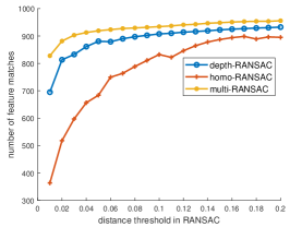
(a)

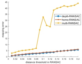
(b)

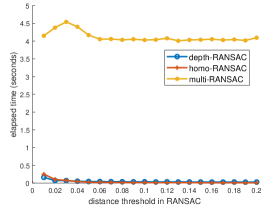
(c)

Figure 3: Comparison of different robust fitting methods on 14 test cases in MVS-Synth Dataset [11]. (a)(b)(c): The average number of feature matches, average mapping error and average elapsed time tested on different distance threshold settings in RANSAC. All the mapping errors are calculated based on Eq. (6).

III-C Image warping via piece-wise homographies

Finally, the warping image $I_{\mathrm{w}}$ is generated by the backward mapping of piece-wise homographies:

$$I_{\mathrm{w}}(\mathbf{x}^{\prime})=I_{\mathrm{t}}\left(\pi\left(\mathrm{H}_{\triangle}^{-1}(\tilde{\mathbf{x}}^{\prime})\right)\right),~{}\forall\mathbf{x}^{\prime}\in\triangle^{\prime},$$ (11)

where $\triangle^{\prime}$ is the triangular domain of $\triangle$ which is forward mapped by $\mathrm{H}_{\triangle}$.

Note that two adjacent domains in $I_{\mathrm{t}}$ may become overlapping in $I_{\mathrm{w}}$ after mapping by different homographies. The implementation details about backward texture mapping by $\{\mathrm{H}_{\triangle}^{-1}\}$ will be presented in Sec. IV-C.

IV Implementation

In this section, we present some implementation details of the proposed method.

IV-A Estimating infinite homography and epipole

In order to estimate $\mathrm{H}_{\infty}$ and $\mathbf{e}^{\prime}$, we firstly prepare a set of SIFT [24] point matches $\{(\mathbf{p}_{i},\mathbf{q}_{i})\}_{i=1}^{N}$ between $I_{\mathrm{t}}$ and $I_{\mathrm{r}}$, a depth map $z=d(\mathbf{x})$ of $I_{\mathrm{t}}$ which can be directly obtained from RGBD datasets.

Similar to the DLT algorithm for estimating homography from a data set $\{(\mathbf{p}_{i},\mathbf{q}_{i})\}_{i=1}^{N}$, $\mathrm{H}_{\infty}$ and $\mathbf{e}^{\prime}$ can be estimated from the augmented data set $\{(\mathbf{p}_{i},\mathbf{q}_{i},d(\mathbf{p}_{i}))\}_{i=1}^{N}$ via solving the following linear least-square problem

$$\min\limits_{\mathbf{h},\mathbf{e}^{\prime}}~{}\left\|\mathrm{A}\,\mathbf{h}+\mathrm{B}\,\mathbf{e}^{\prime}\right\|^{2},$$ (12)

where $\mathbf{h}$ is a $9$-vector made up of the entries of $\mathrm{H}_{\infty}$, and the matrices $\mathrm{A}$ and $\mathrm{B}$ are vertically stacked by

$$\mathrm{A}_{i}=\begin{bmatrix}x_{i}&y_{i}&1&0&0&0&-x_{i}x^{\prime}_{i}&-x^{\prime}_{i}y_{i}&-x^{\prime}_{i}\\ 0&0&0&x_{i}&y_{i}&1&-x_{i}y^{\prime}_{i}&-y_{i}y^{\prime}_{i}&-y^{\prime}_{i}\end{bmatrix}$$

$$\mathrm{B}_{i}=\begin{bmatrix}1/z_{i}&0&-x^{\prime}_{i}/z_{i}\\ 0&1/z_{i}&-y^{\prime}_{i}/z_{i}\end{bmatrix}$$

for $i=1,\ldots,N$, $(x_{i},y_{i})$ and $(x^{\prime}_{i},y^{\prime}_{i})$ are coordinates of $\mathbf{p}_{i}$ and $\mathbf{q}_{i}$, $z_{i}=d(\mathbf{p}_{i})$. When $N\geq 6$, Eq. (12) can be efficiently solved by Singular Value Decomposition (SVD).

For the sake of more robust estimation, we employ the $6$-point SVD solver as the minimal solver in the RANSAC framework. With the help of depth data, a single RANSAC estimator can identify a sufficiently large consensus set of point matches between large parallax views, while existing methods need multiple RANSAC estimators to identify multiple homographies.

Fig. 3 shows the comparison results of the number of feature matches, mapping error and elapsed time via three robust fitting methods: homography-based RANSAC [6] (homo-RANSAC), multiple-sampling RANSAC [31] (multi-RANSAC) and our depth-based RANSAC (depth-RANSAC). The depth-RANSAC method can identify sufficiently many feature matches meanwhile takes the least time and has the lowest mapping error. More experiments on the superiority of our depth-based RANSAC are demonstrated in Sec. V-C.

For the sake of more accurate estimation, $\mathrm{H}_{\infty}$ and $\mathbf{e}^{\prime}$ are refined by solving the following nonlinear LS problem

$$\min\limits_{\mathrm{H}_{\infty},\mathbf{e}^{\prime}}~{}\sum\limits_{i\in\mathrm{IS}}\left\|\pi\left(\mathrm{H}_{\infty}\,\tilde{\mathbf{p}}_{i}+\mathbf{e}^{\prime}/z_{i}\right)-\mathbf{q}_{i}\right\|^{2}$$ (13)

where $\mathrm{IS}$ is the index set of identified inliers from the RANSAC estimator. Eq. (13) can be efficiently solved by the Levenberg-Marquardt (LM) algorithm.

The algorithm for estimating $\mathrm{H}_{\infty}$ and $\mathbf{e}^{\prime}$ is summarized in Algorithm 1.

Algorithm 1 Estimate $\mathrm{H}_{\infty}$ and $\mathbf{e}^{\prime}$.

0:  $\{(\mathbf{p}_{i},\mathbf{q}_{i})\}_{i=1}^{N}$ and $\{z_{i}=d(\mathbf{p}_{i})\}$;

0:  $\hat{\mathrm{H}}_{\infty}$ and $\hat{\mathbf{e}}^{\prime}$.

1:  Initialize $\hat{\mathrm{H}}_{\infty}$, $\hat{\mathbf{e}}^{\prime}$ and $\mathrm{IS}$ via RANSAC with a minimal six-point SVD solver Eq. (12);

2:  Refine $\hat{\mathrm{H}}_{\infty}$ and $\hat{\mathbf{e}}^{\prime}$ by optimizing Eq. (13) with $\mathrm{IS}$;

3:  Return $\hat{\mathrm{H}}_{\infty}$ and $\hat{\mathbf{e}}^{\prime}$.

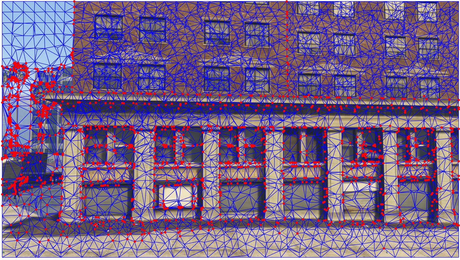
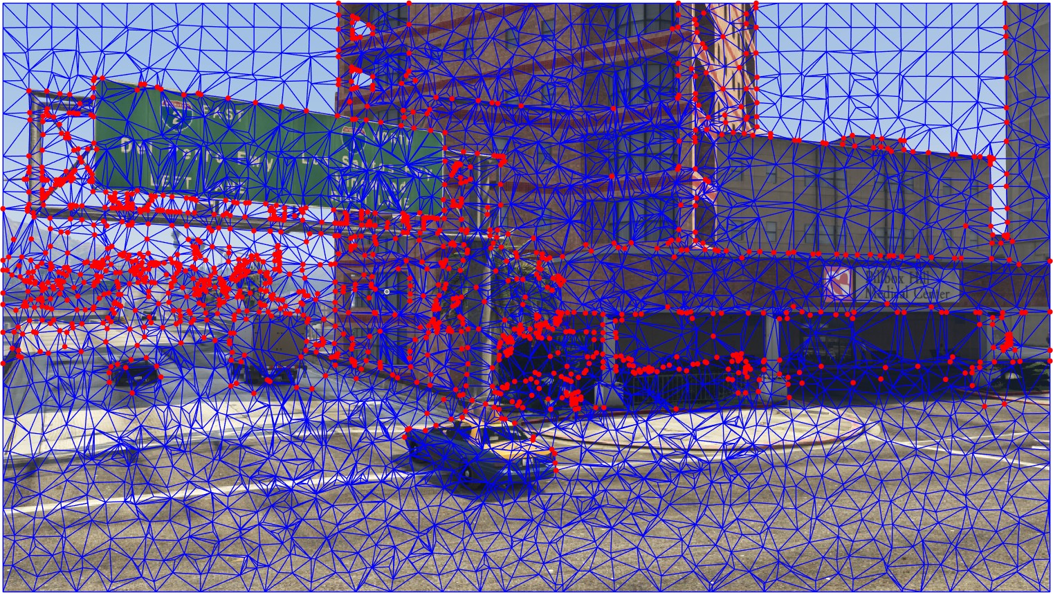
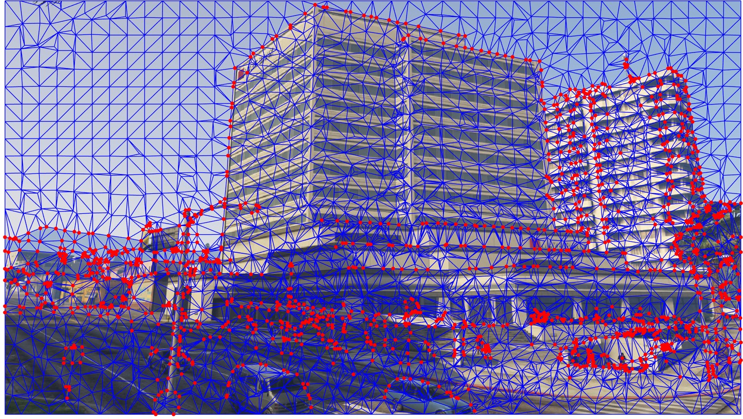
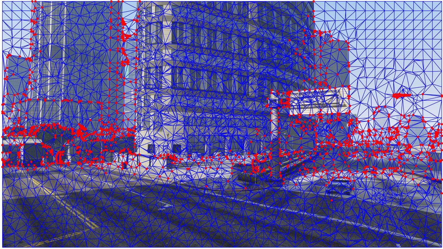
Figure 4: Results of Delaunay triangulation, vertices clustering and backward texture mapping on MVS-Synth Dataset [11]. Test cases from left ro right are (0044, 0064, 0105, 0118), respectively. Red dots in the first row represent the splitting vertices. Black “holes” in the second row indicate the parallax between input images.

IV-B Estimating local homographies

In order to establish multiple local homographies $\{\mathrm{H}_{\triangle}\}$, we first partition the target image into SLIC [1] segments based on its depth map and perform polygonal fitting on the border of each segment. Denote the vertex set by $\{\mathbf{v}_{j}\}_{j=1}^{M}$ consisting of all point matches in the target image and all polygon vertices, then the triangulation can be calculated by the Delaunay triangulation algorithm (see Fig. 2).

IV-B1 Depth rectification of feature points

For the sake of better local alignment, we first rectify the depth value of every matched point $\mathbf{p}_{i}$ by

$$\frac{1}{z_{i}}=\frac{\left(\tilde{\mathbf{y}}^{\prime}\times\mathbf{e}^{\prime}\right)^{T}\left(\tilde{\mathbf{y}}^{\prime}\times\mathrm{H}_{\infty}\tilde{\mathbf{y}}\right)}{\|\tilde{\mathbf{y}}^{\prime}\times\mathbf{e}^{\prime}\|^{2}},$$ (14)

where $(\tilde{\mathbf{y}},\tilde{\mathbf{y}}^{\prime})$ is the corrected point match that minimizes the reprojection error subject to the epipolar constraint, i.e, the optimal solution of

$$\min\limits_{\mathbf{x},\,\mathbf{x}^{\prime}} ~{}~{}~{}\|\mathbf{p}_{i}-\mathbf{x}\|^{2}+\|\mathbf{q}_{i}-\mathbf{x}^{\prime}\|^{2}$$

subject to $$~{}~{}~{}{\tilde{\mathbf{x}}^{\prime T}}\,[\mathbf{e}^{\prime}]_{\times}\,\mathrm{H}_{\infty}\,\tilde{\mathbf{x}}=0.$$

After the above depth rectification, Eq. (8) will enable an optimal three-parameter family of homography for accurate local alignment at the vertex.

IV-B2 Depth rectification of triangle vertices

For the sake of better local naturalness, we then rectify the depth value of every vertex $\mathbf{v}_{j}$, triangle-by-triangle by

$$\frac{1}{z_{j,\triangle}}=\bar{\mathbf{m}}_{\triangle}^{T}\,\tilde{\mathbf{v}}_{j},$$ (15)

where $\bar{\mathbf{m}}_{\triangle}$ is the parameter that best fits the inner points inside the triangle into a plane, i.e., the optimal solution of

$$\min\limits_{\mathbf{m}_{\triangle}}~{}\|\mathrm{C}_{\triangle}\,\mathbf{m}_{\triangle}-\mathbf{d}_{\triangle}\|^{2},$$

where $\mathrm{C}_{\triangle}$ and $\mathbf{d}_{\triangle}$ are stacked vertically by

$$\mathrm{C}_{k}=\begin{bmatrix}x_{k}&y_{k}&1\end{bmatrix},~{}d_{k}=1/z_{k},~{}\forall(x_{k},y_{k})\in\mathrm{int}(\triangle).$$

After the above depth rectification, Eq. (8) will enable an optimal $3$-parameter family of homography for planar local naturalness inside the triangle.

IV-B3 Depth clustering and vertices splitting

In order to enable a globally discontinuous and locally smooth warping model, the multiple rectified depth values of the same vertex should be further clustered and averaged.

Global discontinuity means that one vertex $\mathbf{v}_{j}$ should be allowed to split into some disjointed vertices after warping. For multiple depth values of a vertex, if the maximal difference is less than a threshold $\eta$, we consider them to be of the same class, otherwise we cluster them into different classes via a multiple-model fitting method [12], i.e.,

$$\min_{\mathbf{L}}E(\mathbf{L})=\sum_{p}\|p-L_{p}\|+\beta\cdot|\mathcal{L}_{\mathbf{L}}|.$$ (16)

Fig. 4 shows some experimental results of vertices clustering and splitting.

Local smoothness means that those triangles sharing a common vertex after warping should share the same depth value at this common vertex before warping. Therefore, we assign the average of multiple depth values inside their member class to the common vertex. Note that, for the class that includes the rectified depth value of a matched feature point, we assign that value rather than the average to the common vertex, such that the feature point can be prior aligned.

The algorithm for estimating $\{\mathrm{H}_{\triangle}\}$ for triangles is summarized in Algorithm 2.

Algorithm 2 Estimate $\{\mathrm{H}_{\triangle}\}$.

0:  $\{\triangle\}$, $\{(\mathbf{p}_{i},\mathbf{q}_{i})\}_{i\in\mathrm{IS}}$ and $d(I)$;

0:  $\{\mathrm{H}_{\triangle}\}$.

1:  For every $\mathbf{p}_{i}$, rectify its depth value by Eq. (14);

2:  For every $\triangle$, rectify the depth value of $\mathbf{v}_{j}$ by Eq. (15);

3:  For every $\mathbf{v}_{j}$, cluster its multiple depth values;

4:  For every $\triangle$, finalize the depth value of $\mathbf{v}_{j}$ as the average of its member class then solve Eq. (8) to get $\mathbf{m}_{\triangle}$;

5:  Return $\{\mathrm{H}_{\triangle}\}$ that formulated by Eq. (10) with $\{\mathbf{m}_{\triangle}\}$.

(a) 0002

(b) 0016

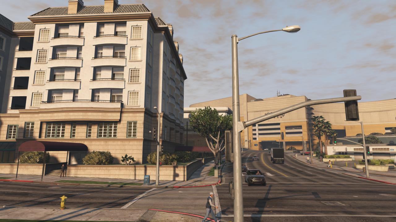
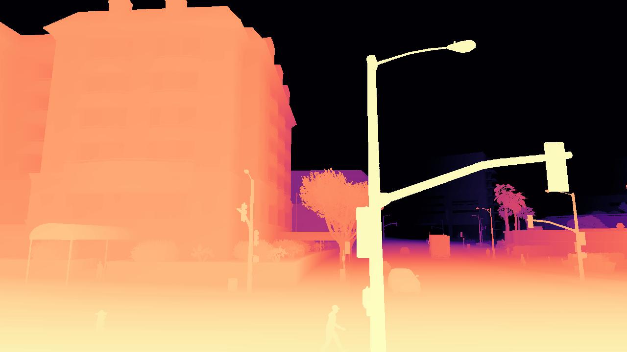
(c) 0022

(d) 0044

(e) 0047

(f) 0064

(g) 0079

(h) 0090

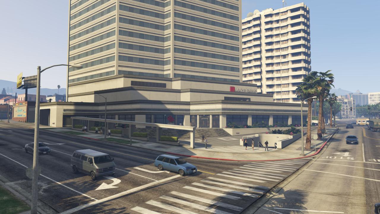
(i) 0105

(j) 0118

Figure 5: Dataset for quantitative comparison.

IV-C Backward texture mapping

Since vertices splitting is allowed, the splitting triangles may be overlapping with each other in the overlapping region and even the non-overlapping region. When such case happens, i.e. two different local homographies $\mathrm{H}_{\triangle}$ and $\mathrm{H}_{\triangle^{\prime}}$ map two different point $\mathbf{p}$ and $\mathbf{p}^{\prime}$ in $I_{\mathrm{t}}$ to the same point $\mathbf{q}$ in $I_{\mathrm{w}}$, we compare $d(\mathrm{H}_{\triangle}^{-1}(\tilde{\mathbf{q}}))$ with $d(\mathrm{H}_{\triangle^{\prime}}^{-1}(\tilde{\mathbf{q}}))$ and use the pixel with the smaller depth value in the backward texture mapping, because it is closer to camera.

After images are warped and rendered, we blend them together via average blending to produce the final panorama. However, due to the large parallax between input images, the panorama may still have missing “holes” in the non-overlapping region (see Fig. 4), which are eliminated by applying image inpainting algorithms [5, 15] to the missing regions.

Finally, we summarize our method in Algorithm 3.

Algorithm 3 Natural Image Stitching using Depth Maps.

0:  $I_{\mathrm{t}}$ and $I_{\mathrm{r}}$;

0:  Panorama $I_{\mathrm{m}}$.

1:  Extract a depth map of $I_{\mathrm{t}}$;

2:  Extract a set of point matches between $I_{\mathrm{t}}$ and $I_{\mathrm{r}}$;

3:  Extract a triangulation of $I_{\mathrm{t}}$;

4:  Estimate $\mathrm{H}_{\infty}$ and $\mathbf{e}^{\prime}$ via Algorithm 1;

5:  Estimate $\{\mathrm{H}_{\triangle}\}$ via Algorithm 2;

6:  Warp $I_{\mathrm{t}}$ to $I_{\mathrm{w}}$ via backward texture mapping;

7:  Composite $I_{\mathrm{w}}$ and $I_{\mathrm{r}}$ via average blending to create $I_{\mathrm{m}}$;

8:  Apply image inpainting method to panorama $I_{m}$ to fill the missing holes.

V Experiments

A series of comparison experiments are conducted to evaluate the performance of our proposed NIS method. The comparing methods include global homography (Homo), APAP [31], NISwGSP [4] and LFA [17]. The parameters of existing methods are set as suggested by the original papers. In the experiment, we use VLFeat [28] to extract and match SIFT [24] feature points, use our robust fitting algorithm to remove outliers. To ensure a fair comparison, the same matching data are used in all tested methods except the NISwGSP method which is implemented in C++. To highlight the accuracy of image alignment, all stitching results are generated via simple average blending.

TABLE I: Comparisons on MS-SSIM and PSNR.

Dataset	MS-SSIM $\uparrow$ / PSNR $\uparrow$
	Homo	APAP [31]	NISwGSP [4]	LFA [17]	Ours
0002	0.8206/18.8346	0.8944/19.9026	0.9281/20.3518	0.8404/19.3579	0.9328/24.3715
0016	0.6108/15.8300	0.8277/18.9876	0.8028/17.9444	0.8359/19.0841	0.8979/21.9402
0022	0.6399/17.3369	0.8014/19.9049	0.8025/19.7191	0.7051/18.4067	0.9220/23.9084
0044	0.4546/15.8437	0.8200/21.3852	–	0.7812/20.5869	0.9351/25.2064
0047	0.5134/16.7394	0.6564/18.9894	0.6232/18.0361	0.6277/17.7134	0.9158/22.6412
0064	0.5623/17.6217	0.8377/21.1313	0.8597/21.5153	0.9169/23.8954	0.9224/24.5517
0079	0.5207/16.4707	0.8353/20.8725	0.8490/20.5486	0.6298/17.4495	0.9333/24.5749
0090	0.6906/18.0152	0.8825/21.7101	0.8678/21.4278	0.8080/20.3467	0.9248/23.2854
0105	0.8928/22.1935	0.9468/24.7182	0.9543/25.7275	0.8496/20.8186	0.9362/23.4227
0118	0.6019/19.1429	0.9314/24.9119	–	0.6859/20.6206	0.9284/25.3247
Average	0.6308/17.8029	0.8434/21.2514	0.8359/20.6588	0.7681/19.8262	0.9249/23.9227

V-A Quantitative comparison

In order to accurately evaluate the performance of our NIS method, we introduce two indices, MS-SSIM (Multiscale structural similarity) [29] and PSNR to evaluate the alignment quality and compare with other methods. The image dataset used in the quantitative experiments is exhibited in Fig. 5, which is selected from MVS-Synth Dataset [11]. The MS-SSIM and PSNR indices are calculated based on the overlapping regions of warped images.

The scores of different methods are listed in Table I. In some test cases, NISwGSP [4] fails to align the images naturally, resulting in severe misalignments and meaningless indices, which are indicated as “–”. The global homography (Homo) is not able to handle the large parallax and eliminate local structure misalignments, such that receives the lowest scores. The three existing methods could achieve better alignment quality, hence get higher scores. Among all the tested methods, our proposed NIS method achieves the highest scores in most cases, and therefore provides the best alignment quality. It’s worth noting that, though our method receives the lower score in 0105 test case, there are still non-negligible misalignments in the other methods, which the two indices may fail to identify (see Fig. 6).

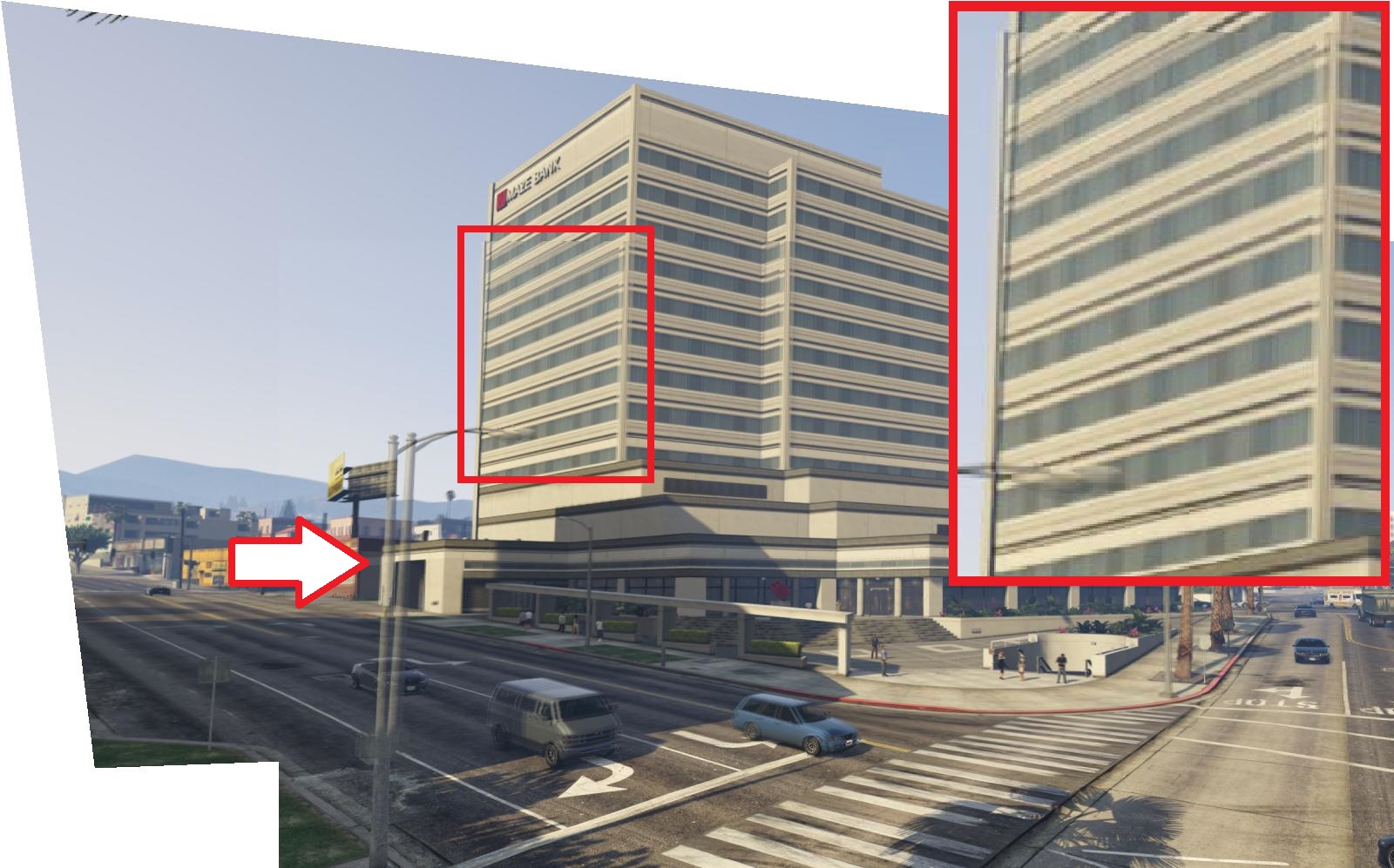
(a) Homography

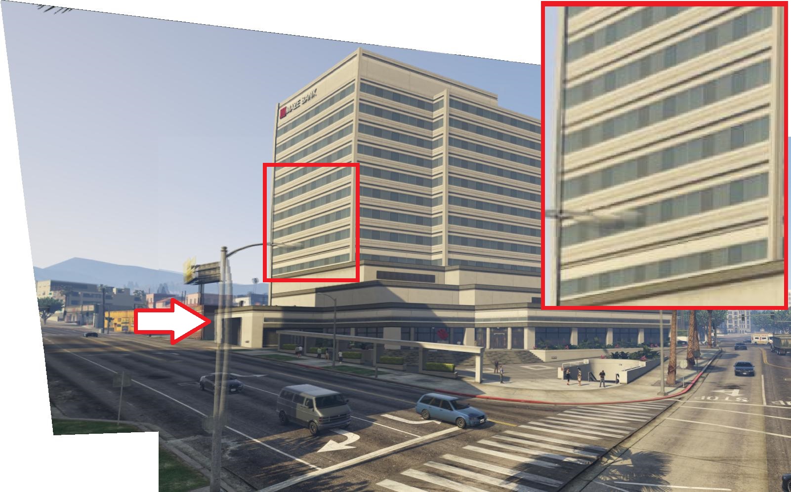
(b) APAP [31]

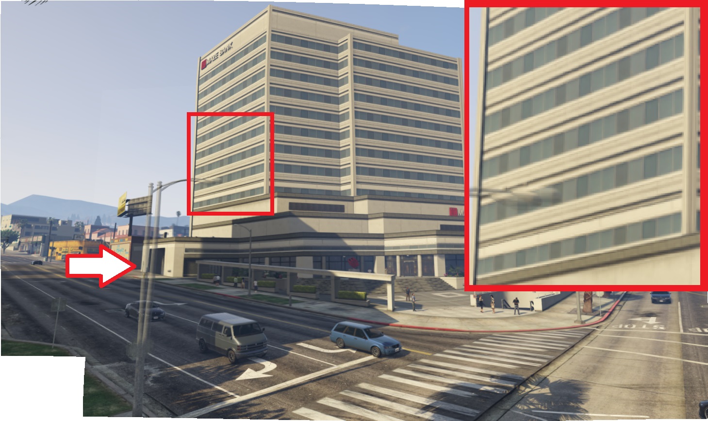
(c) NISwGSP [4]

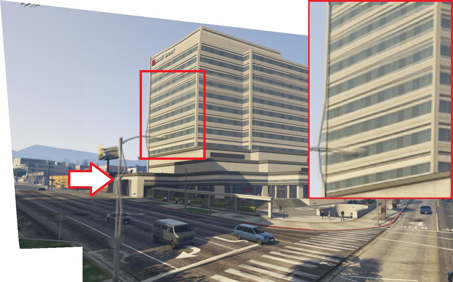
(d) LFA [17]

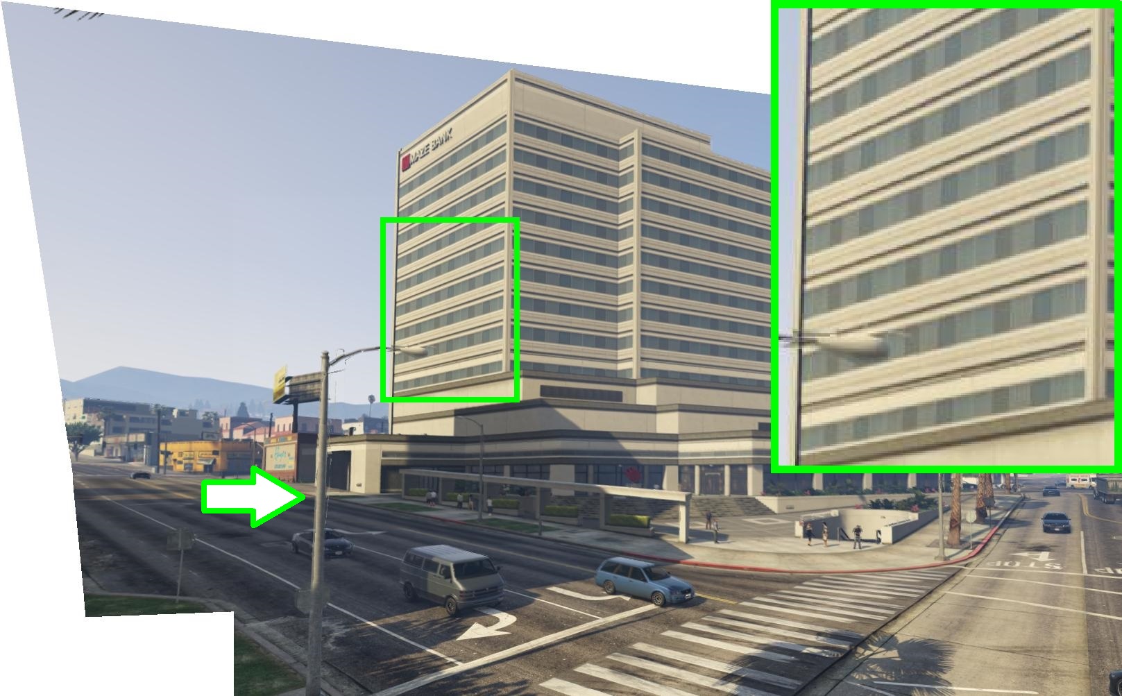
(e) Our method

Figure 6: Comparisons with state-of-the-art image stitching methods on the 0105 test case (best view in color and zoom in).

V-B Qualitative comparison

Fig. 6 demonstrates the comparison results of the 0105 test case, which contains drastically varying depth. Two representative areas in the overlapping region of each panorama are highlighted with colored boxes and arrows. Due to the lack of matching data on the street lamp, the four existing methods suffer severe ghosting effects (see red arrows), global homography and LFA cannot align the building, while APAP and NISwGSP can relieve the structure misalignments (see red boxes). With the help of the depth map, our local warping model can accurately align the street lamp and building, hence outperforms all the other methods. More comparison results on other test cases are provided in the supplementary material.

V-C Ablation study

We validate the effectiveness of every module in our method by evaluating the average measures of the 10 test cases in Fig. 5, as shown in Table II.

TABLE II: Ablation studies on MVS-Synth Dataset [11].

	Robust fitting			Depth rectification			Metric
	Homo-RANSAC	Multi-RANSAC	Depth-RANSAC	w/ Eq. (14)	w/ Eq. (15)	w/ Eq. (16)	MS-SSIM $\uparrow$	PSNR $\uparrow$
1	✓			✓	✓	✓	0.6870	17.5890
2		✓		✓	✓	✓	0.8579	22.0899
3			✓	✓	✓	✓	0.9249	23.9227
4			✓	✓	✓		0.9264	23.9095
5			✓	✓			0.8520	20.7023
6			✓				0.8522	20.7059

V-C1 Robust fitting

We test different robust fitting methods, homography-based RANSAC (homo-RANSAC), multiple-sampling RANSAC (multi-RANSAC) and our depth-based RANSAC (depth-RANSAC), as shown in the experiments 1-3 of Table II. The homo-RANSAC cannot identify sufficient matched features for large parallax cases, thus provides the lowest alignment accuracy. Although, the multi-RANSAC identified sufficient features as our depth-RANSAC, it has the lower accuracy than ours. We believe the reason is that the multi-RANSAC has the worst mapping error (see Fig. 3(b)) such that the subsequent local warping cannot alleviate it.

V-C2 Depth rectification

We ablate the depth rectification module in Sec. IV-B as the basic structure and evaluate the effectiveness of different rectification equations (Eqs. (14,15,16)). As shown in experiments 3-6 of Table II, the basic structure (experiment 6) means that all the local homographies are estimated based on the depth values of the triangle vertices, the experiment 4 means that all the rectified depth values are not clustered and averaged. The comparison results shows that the depth rectification of triangle vertices can significantly improve the alignment accuracy, even achieves the best MS-SSIM score. Noting that experiments 3-4 shows that the depth clustering and averaging may have little effect on improving the alignment accuracy of the overlapping region, but it can help generating a locally smoother panorama in the non-overlapping region. Fig. 7 demonstrates a comparison of 0118 test case. The warped target image of experiment 4 has too much splitting issues (see Fig. 7(a) the mask image), while the final model can relieve such issues.

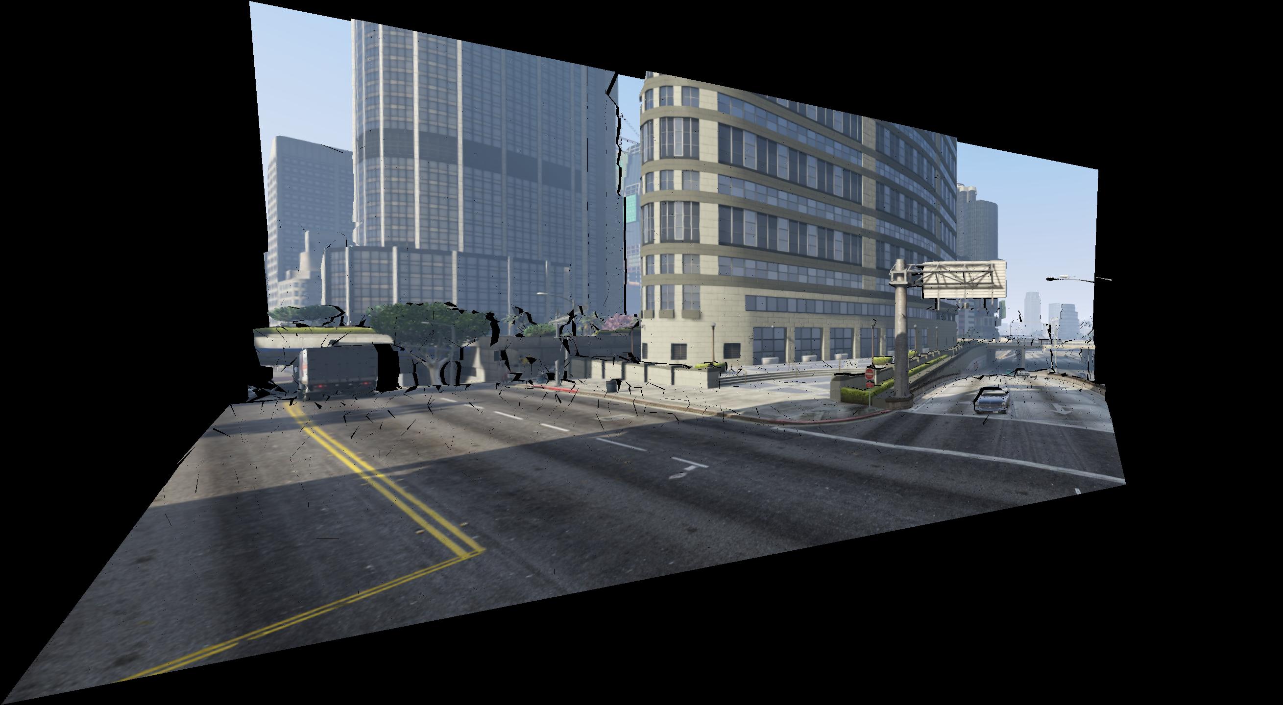
(a) Warped target via experiment 4 of the ablation study

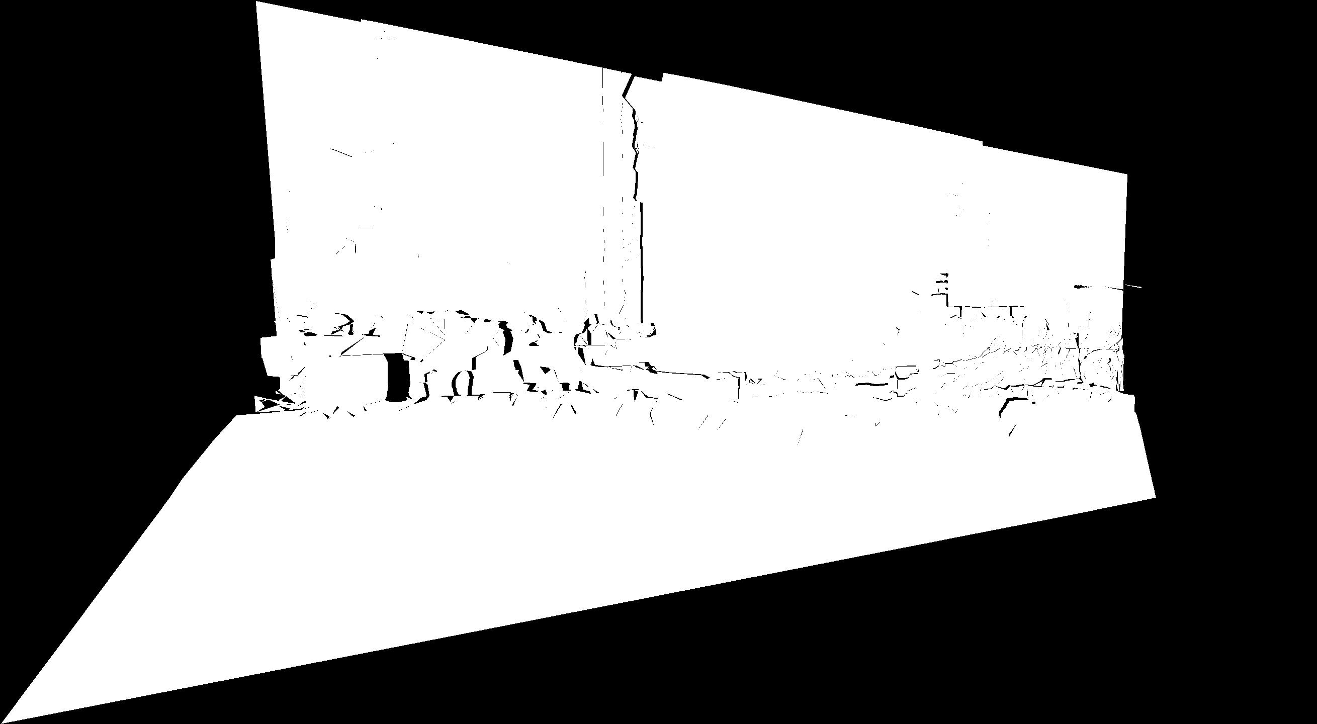
(b) Warped target via our final model

Figure 7: Comparison of warped target images of the 0118 test case. In (a),(b), Left is the warped target images; Right is the masks of the warped target images.

V-D Limitation and failure examples

Our method assumes that the depth map of the target image is relatively accurate, the triangulation of the target image is assumed to be coplanar in the space for every triangular domain. Furthermore, the missing area in the panorama should not be too large. If such assumptions are violated, our method may fail to generate a plausible result.

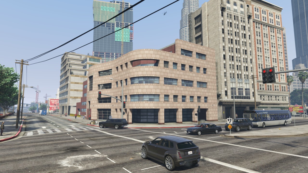
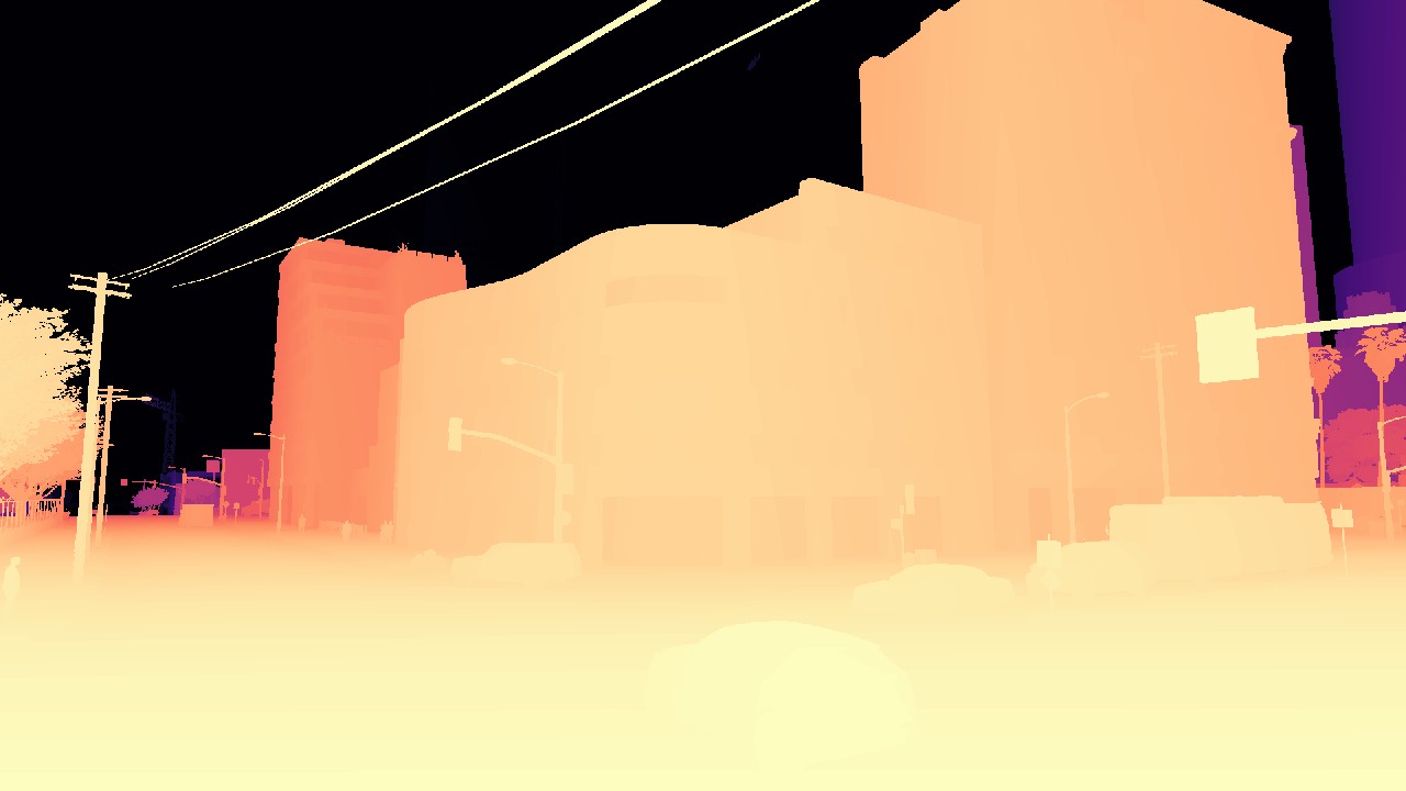
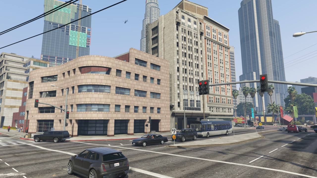
(a) Input images and depth map of target

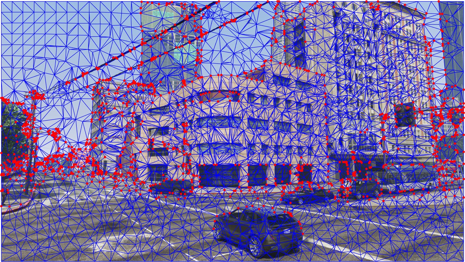
(b) Warped target image

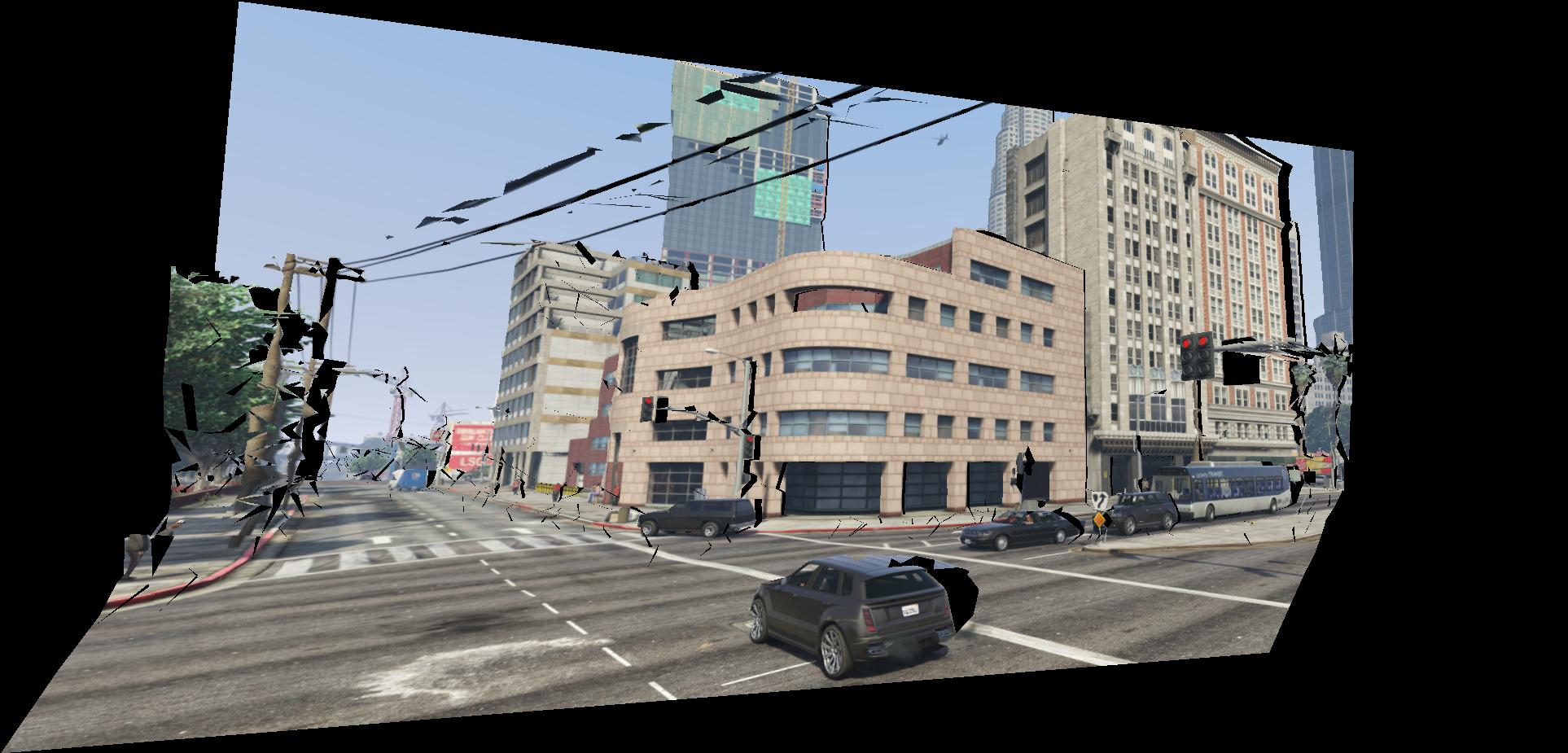
(c) Warped target image

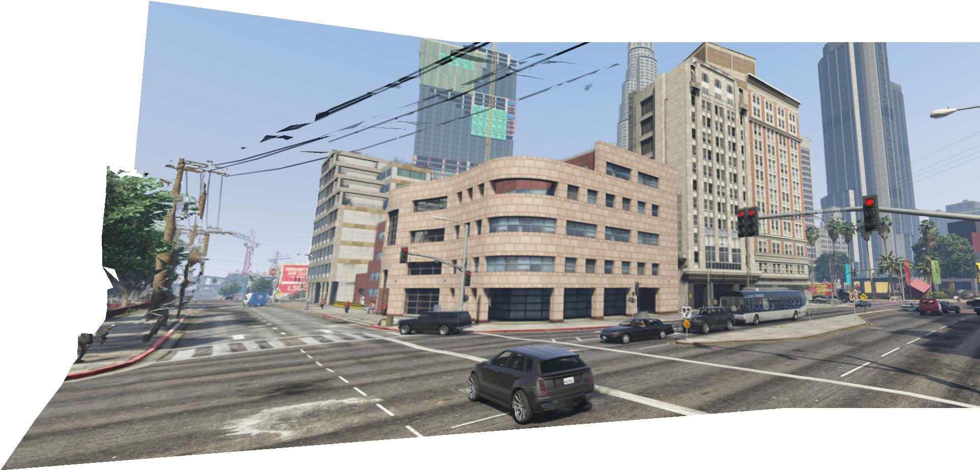
(d) Final panorama

Figure 8: Failure example of a test case in MVS-Synth Dataset [11].

Fig. 8 shows a failure example of our proposed method. Input images are of wide camera baseline and drastic depth variation. Due to the abundant and complex geometric structures, the Delaunay triangulation and the subsequent depth values clustering are error-prone (see Fig. 8(b-c)), and then ghosting or artifacts introduced by blending or image inpainting appear in the resulting panorama.

VI Conclusion

This paper proposes a natural image stitching (NIS) method using depth maps. Our main contribution is to provide an adaptive method that leverages depth maps in NIS to address the challenge of parallax. Experimental results show that the proposed method not only provides accurate alignment in the overlapping regions, but also virtual naturalness in the non-overlapping region. Future research includes reducing the dependence on the depth map, and designing a more accurate and less complex triangulation algorithm.

References

- [1] Radhakrishna Achanta, Appu Shaji, Kevin Smith, Aurelien Lucchi, Pascal Fua, and Sabine Süsstrunk. Slic superpixels compared to state-of-the-art superpixel methods. IEEE Trans. Pattern Anal. Mach. Intell., 34(11):2274–2282, 2012.
- [2] Che-Han Chang, Yuuki Sato, and Yung-Yu Chuang. Shape-preserving half-projective warps for image stitching. In IEEE Conf. Comput. Vis. Pattern Recog., pages 3254–3261, 2014.
- [3] Shenchang Eric Chen and Lance Williams. View interpolation for image synthesis. In Proceedings of the 20th Annual Conference on Computer Graphics and Interactive Techniques, SIGGRAPH ’93, page 279–288, New York, NY, USA, 1993. Association for Computing Machinery.
- [4] Yu-Sheng Chen and Yung-Yu Chuang. Natural image stitching with the global similarity prior. In Eur. Conf. Comput. Vis., pages 186–201, 2016.
- [5] Antonio Criminisi, Patrick Pérez, and Kentaro Toyama. Region filling and object removal by exemplar-based image inpainting. IEEE Transactions on image processing, 13(9):1200–1212, 2004.
- [6] Martin A Fischler and Robert C Bolles. Random sample consensus: a paradigm for model fitting with applications to image analysis and automated cartography. Communications of the ACM, 24(6):381–395, 1981.
- [7] Junhong Gao, Seon Joo Kim, and Michael S Brown. Constructing image panoramas using dual-homography warping. In IEEE Conf. Comput. Vis. Pattern Recog., pages 49–56, 2011.
- [8] Junhong Gao, Yu Li, Tat-Jun Chin, and Michael S Brown. Seam-driven image stitching. Eurographics, pages 45–48, 2013.
- [9] Clement Godard, Oisin Mac Aodha, Michael Firman, and Gabriel J. Brostow. Digging into self-supervised monocular depth estimation. In Int. Conf. Comput. Vis., October 2019.
- [10] R. I. Hartley and A. Zisserman. Multiple View Geometry in Computer Vision. Cambridge University Press, second edition, 2004.
- [11] Po-Han Huang, Kevin Matzen, Johannes Kopf, Narendra Ahuja, and Jia-Bin Huang. Deepmvs: Learning multi-view stereopsis. In IEEE Conference on Computer Vision and Pattern Recognition (CVPR), 2018.
- [12] Hossam Isack and Yuri Boykov. Energy-based geometric multi-model fitting. Int. J. Comput. Vis., 97(2):123–147, 2012.
- [13] Qi Jia, ZhengJun Li, Xin Fan, Haotian Zhao, Shiyu Teng, Xinchen Ye, and Longin Jan Latecki. Leveraging line-point consistence to preserve structures for wide parallax image stitching. In IEEE Conf. Comput. Vis. Pattern Recog., pages 12186–12195, June 2021.
- [14] K. Joo, N. Kim, T. Oh, and I. S. Kweon. Line meets as-projective-as-possible image stitching with moving dlt. In IEEE Int. Conf. Image Process., pages 1175–1179, 2015.
- [15] Olivier Le Meur, Mounira Ebdelli, and Christine Guillemot. Hierarchical super-resolution-based inpainting. IEEE transactions on image processing, 22(10):3779–3790, 2013.
- [16] Kyu-Yul Lee and Jae-Young Sim. Warping residual based image stitching for large parallax. In IEEE Conf. Comput. Vis. Pattern Recog., June 2020.
- [17] Jing Li, Baosong Deng, Rongfu Tang, Zhengming Wang, and Ye Yan. Local-adaptive image alignment based on triangular facet approximation. IEEE Trans. Image Process., 29:2356–2369, 2019.
- [18] N. Li, Y. Xu, and C. Wang. Quasi-homography warps in image stitching. IEEE Trans. Multimedia, 20(6):1365–1375, 2018.
- [19] Shiwei Li, Lu Yuan, Jian Sun, and Long Quan. Dual-feature warping-based motion model estimation. In Int. Conf. Comput. Vis., pages 4283–4291, 2015.
- [20] T. Liao and N. Li. Single-perspective warps in natural image stitching. IEEE Trans. Image Process., 29:724–735, 2020.
- [21] Chung-Ching Lin, Sharathchandra U Pankanti, Karthikeyan Natesan Ramamurthy, and Aleksandr Y Aravkin. Adaptive as-natural-as-possible image stitching. In IEEE Conf. Comput. Vis. Pattern Recog., pages 1155–1163, 2015.
- [22] Kaimo Lin, Nianjuan Jiang, Loong-Fah Cheong, Minh Do, and Jiangbo Lu. Seagull: Seam-guided local alignment for parallax-tolerant image stitching. In Eur. Conf. Comput. Vis., pages 370–385, 2016.
- [23] Kaimo Lin, Nianjuan Jiang, Shuaicheng Liu, Loong-Fah Cheong, Minh Do, and Jiangbo Lu. Direct photometric alignment by mesh deformation. In IEEE Conf. Comput. Vis. Pattern Recog., pages 2701–2709. IEEE, 2017.
- [24] David G Lowe. Distinctive image features from scale-invariant keypoints. Int. J. Comput. Vis., 60(2):91–110, 2004.
- [25] Eric Penner and Li Zhang. Soft 3d reconstruction for view synthesis. ACM Trans. Graph., 36(6), Nov. 2017.
- [26] Meng-Li Shih, Shih-Yang Su, Johannes Kopf, and Jia-Bin Huang. 3d photography using context-aware layered depth inpainting. In IEEE Conf. Comput. Vis. Pattern Recog., pages 8025–8035, 2020.
- [27] Richard Szeliski. Image alignment and stitching: A tutorial. Foundations and Trends® in Computer Graphics and Vision, 2(1):1–104, 2006.
- [28] Andrea Vedaldi and Brian Fulkerson. Vlfeat: An open and portable library of computer vision algorithms. In Proceedings of the 18th ACM International Conference on Multimedia, pages 1469–1472, 2010.
- [29] Zhou Wang, Eero P Simoncelli, and Alan C Bovik. Multiscale structural similarity for image quality assessment. In The Thrity-Seventh Asilomar Conference on Signals, Systems & Computers, 2003, volume 2, pages 1398–1402. IEEE, 2003.
- [30] Olivia Wiles, Georgia Gkioxari, Richard Szeliski, and Justin Johnson. Synsin: End-to-end view synthesis from a single image. In IEEE Conf. Comput. Vis. Pattern Recog., pages 7465–7475, 2020.
- [31] Julio Zaragoza, Tat-Jun Chin, Quoc-Huy Tran, Michael S Brown, and David Suter. As-projective-as-possible image stitching with moving dlt. IEEE Trans. Pattern Anal. Mach. Intell., 7(36):1285–1298, 2014.
- [32] Fan Zhang and Feng Liu. Parallax-tolerant image stitching. In IEEE Conf. Comput. Vis. Pattern Recog., pages 3262–3269, 2014.
- [33] Guofeng Zhang, Yi He, Weifeng Chen, Jiaya Jia, and Hujun Bao. Multi-viewpoint panorama construction with wide-baseline images. IEEE Trans. Image Process., 25(7):3099–3111, 2016.
- [34] J. Zheng, Y. Wang, H. Wang, B. Li, and H. M. Hu. A novel projective-consistent plane based image stitching method. IEEE Trans. Multimedia, 21(10):2561–2575, 2019.
- [35] Tinghui Zhou, Richard Tucker, John Flynn, Graham Fyffe, and Noah Snavely. Stereo magnification: Learning view synthesis using multiplane images. ACM Trans. Graph., 37(4), July 2018.