Critical-layer instability of shallow water magnetohydrodynamic shear flows

Abstract

In this paper, the instability of shallow water shear flow with a sheared parallel magnetic field is studied. Waves propagating in such magnetic shear flows encounter critical levels where the phase velocity relative to the basic flow $c-U(y)$ matches the Alfvén wave velocities $\pm B(y)/\sqrt{\mu\rho}$, based on the local magnetic field $B(y)$, the magnetic permeability $\mu$ and the mass density of the fluid $\rho$. It is shown that when the two critical levels are close to each other, the critical layer can generate an instability. The instability problem is solved, combining asymptotic solutions at large wavenumbers and numerical solutions, and the mechanism of instability explained using the conservation of momentum. For the shallow water MHD system, the paper gives the general form of the local differential equation governing such coalescing critical layers for any generic field and flow profiles, and determines precisely how the magnetic field modifies the purely hydrodynamic stability criterion based on the potential vorticity gradient in the critical layer. The curvature of the magnetic field profile, or equivalently the electric current gradient, $J^{\prime}=-B^{\prime\prime}/\mu$ in the critical layer is found to play a complementary role in the instability.

1 Introduction

The shallow water equations are an essential idealised model for the study of large-scale dynamics in geophysical fluid systems. Their relatively simple form has provided significant insights in our understanding of waves, instabilities and turbulence in the oceans and atmosphere. More recently, Gilman (2000) extended the application of the shallow water model to the dynamics of the solar tachocline by incorporating a magnetic field. In the present study, we will examine the stability of such shallow water magnetohydrodynamic (MHD) systems.

The stability properties of hydrodynamic shallow water flows have been studied extensively, and we now know of a number of instabilities with distinctive features. They include Rayleigh’s instability which is related to an inflectional point of the shear flow profile (Blumen et al., 1975), resonant instability generated by interaction between two neutral modes (Satomura, 1981; Hayashi & Young, 1987), critical-layer instability induced by singularities of neutral modes (Balmforth, 1999; Riedinger & Gilbert, 2014), and radiative instability caused by waves radiating outward in an unbounded domain (Ford, 1994; Riedinger & Gilbert, 2014).

In the context of astrophysical flows, such as in the solar tachocline, magnetic fields are present and will generally modify the stability properties of the flow. Although the elasticity of field lines suggests a stabilising effect, in reality this additional coupling can lead to new modes of instability, as occurs for example in the magneto-rotational instability (Balbus and Hawley 1991). The instability of two-dimensional shear flow with a parallel magnetic field has been investigated by a number of researchers. It is well known that a strong magnetic field has a stabilizing effect. Chandra (1973) and Hughes & Tobias (2001) have shown that modified versions of Howard’s (1961) semicircle rule exist when the field is included. The magnetic field reduces the possible domain in which the complex phase velocity may reside, and instability will be suppressed if the magnetic field is sufficiently strong everywhere.

The role of a weaker magnetic field, however, is more subtle, and researchers have found situations where it may have a destabilising effect. Kent (1968), Stern (1963) and Chen & Morrison (1991) have studied the instability problem analytically in the zero-wavenumber limit, in which case the dispersion relation reduces to an equation involving a simple integral. They have demonstrated various examples where the magnetic field may destabilise an otherwise stable flow, e.g., a parabolic profile of the field can destabilise a plane Couette flow (Chen & Morrison, 1991). Guided by these theoretical studies, Tatsuno & Dorland (2006), Lecoanet et al. (2010) and Heifetz et al. (2015) have computed unstable modes numerically at finite small wavenumbers.

The instability of shallow water MHD systems has been studied by Mak et al. (2016). They consider basic velocity profiles of unstable shear layers and jets, and examine the effect of a uniform magnetic field on these classical instabilities. Their results demonstrate that the field mainly plays a stabilising role. The same semicircle rule of Hughes & Tobias (2001) exists, so a sufficiently strong magnetic field can suppress any instability. Increasing the field always reduces the maximum unstable growth rate, but in some situations may increase the (albeit small) growth rates for long wavelength modes.

The instability analyses cited so far are all based on flows in Cartesian geometry, but for the solar tachocline, spherical geometry is a better representation. Gilman & Fox (1997, 1999) considered two-dimensional MHD flows in a thin spherical shell with the basic differential rotation profile of the Sun and various magnetic fields. They found a ‘joint instability’: either the shear flow or the magnetic field is stable by itself, but the system is unstable when they are present together. Gilman & Dikpati (2002) and Dikpati et al. (2003) studied the effect of a free surface on these joint instabilities by employing the shallow water MHD model of Gilman (2000). They show that the free surface has a weak effect on the instability as long as the effective gravity is not too small, but as this parameter is decreased the instability is eventually completely suppressed as the shell thickness of the reference state tends to zero at certain latitudes. Márquez-Artavia et al. (2017) revealed yet another type of instability for shallow-water MHD flow on a sphere: it is purely induced by the free surface and the magnetic field, and exists even when the basic flow is quiescent or is solid-body rotation. A review of MHD instabilities in spherical shells has been given by Gilman & Cally (2007). The consequences of these instabilities may include transition to turbulence, magnetic reconnection (Cally, 2001; Cally et al., 2003), and the generation of Rossby waves in the solar tachocline (Dikpati & McIntosh, 2020).

In the present study, we investigate the effect of critical levels on the instability of shallow water MHD systems. Critical levels appear as singularities of steady waves propagating in shear flows if the fluid system has no dissipation. In hydrodynamic problems with flow profile $U(y)$, say, a critical level is a location $y=y_{{c}}$ at which the phase velocity of waves matches the basic flow velocity, i.e. $c=U(y)$. When a parallel magnetic field is added, the critical levels become locations $y=y_{B\pm}$ where $c-U(y)$ matches the Alfvén wave velocity $\pm B(y)/\sqrt{\rho\mu}$, where $B(y)$ is the magnetic field profile, $\rho$ is the mass density of the fluid and $\mu$ is the magnetic permeability. These magnetic critical layers have been found to play crucial roles in a wide range of phenomena and applications, including sunspots (Sakurai et al., 1991), solar wind (Chen & Hasegawa, 1974), hot Jupiters (Hindle et al., 2021) and tokamak reactors (Mok & Einaudi, 1985).

In hydrodynamic stability theory, critical layers play the key role in driving instabilities in a wide variety of flows. They include the shallow water flows we have mentioned, baroclinic flows (Bretherton, 1966), stratified flows with horizontal shear (Wang & Balmforth, 2018), and, perhaps most famously, wind flowing over water generating surface water waves (Miles, 1957). All these instabilities share a common mechanism: the critical layer generates a finite amount of mean-flow momentum (or potential vorticity, equivalently). Thus, given the total momentum is conserved, the mean-flow momentum in the critical layer must be balanced by unsteady motion in the outer flow, and this balance can be thought of as driving the instability.

Therefore, these instabilities are sometimes referred to as ‘critical-layer instabilities’ (Bretherton, 1966; Riedinger & Gilbert, 2014). However, the magnetic field-induced instabilities found in previous studies cannot be understood in terms of this mechanism. For example, in Tatsuno & Dorland (2006), Lecoanet et al. (2010) and Heifetz et al. (2015), it can be inferred that the mean-flow modification is anti-symmetric due to the parity property of the unstable modes. As a result the mean-flow momentum generated in two critical layers cancels out completely and so cannot be seen to drive the growth of the outer flow. Instead, the instability may be interpreted as a result of adding more magnetic free energy to the system (Lecoanet et al., 2010) or through the interaction between vorticity waves (Heifetz et al., 2015).

In this paper, we will reveal a new kind of magnetic critical layer instability in shallow water MHD systems. It shares a similar mechanism with the hydrodynamic critical layer instabilities, but magnetic critical levels have distinctive properties. Unlike hydrodynamic instabilities where there is usually a single critical level, here we have two critical levels close to each other, and hence their interaction plays a crucial role in the instability. Also, in the hydrodynamic shallow water system, the potential vorticity (PV) is conserved and it largely controls the dynamics of the flow. In particular, the sign of the background potential vorticity gradient $Q^{\prime}=-(U^{\prime}/H)^{\prime}$ ($H$ being the depth of shallow water) determines whether the critical layer has a stabilising or destabilising effect (Balmforth, 1999; Riedinger & Gilbert, 2014). A magnetic field, however, breaks the PV conservation and significantly changes the dynamics. An example of the impact of such a loss of PV conservation has been presented by Dritschel et al. (2018) for the fundamental problem of the evolution of two-dimensional vortices. We will show that the loss of PV conservation has a dramatic impact on the MHD shallow water system as well: this is evident in the study of the basic flow of linear shear, i.e.  vanishing background vorticity gradient $-U^{\prime\prime}(y)=0$, and a constant shallow-water depth $H$. In the absence of a magnetic field, PV conservation would imply there is no critical level at all. The presence of a magnetic field, however, brings back the singular behaviour at the critical levels, and hence the possibility of critical layer instability. The general instability criterion we obtain combines the PV gradient $Q^{\prime}$ with the analogous quantity of the electric current gradient $J^{\prime}=-B^{\prime\prime}/\mu$ in a key ‘curvature parameter’ $\gamma$ which appears in the local ODE for the critical layer.

Finally, we investigate the mean-flow response of the instability, and show that it is strongly localised in the critical layer. We explain the instability mechanism via the conservation of momentum following the paradigm of Hayashi & Young (1987), which is a balance between the ‘mean momentum’ and the ‘wave momentum’. The mean momentum is just the momentum of mean-flow response, while the ‘wave momentum’ is the coupling between linear waves of velocity and surface displacements. We show that the mean momentum generated in the critical layer must be balanced by the exponential growth of the wave momentum, and this can be understood as a mechanism for the instability. This mechanism is similar to that of hydrodynamic critical layer instabilities, but we will show that the magnetic field also controls the mean momentum via the Maxwell stress and the electric current gradient $J^{\prime}=-B^{\prime\prime}/\mu$.

The layout of the paper is as follows. In §2, we present the equations for the problem. The shallow water magnetohydrodynamic system of Gilman (2000) is given in §2.1, the eigenvalue problem for the linear instability is derived in §2.2, and the equations for the mean-flow responses and momentum conservation are obtained in §2.3. In §3, we present numerical solutions to the instability problem and the mean-flow response for typical basic-flow profiles, and summarise the instability criterion and the instability mechanism. In §4, we derive the asymptotic solution for the instability problem at large wavenumbers for general basic-flow profiles, and explain the instability mechanism via momentum conservation. We conclude in §5 and compare the new instability to those discussed in the literature.

2 The governing equations

2.1 The shallow water MHD model

We study the dynamics of the shallow water magnetohydrodynamic (SWMHD) model for ideal, perfectly conducting fluid originally proposed by Gilman (2000). Our main objective is to study the effect of critical levels on stability, and as a starting point we use Cartesian coordinates which are easier for analysis. Let $(x,y)$ be the horizontal coordinates and $z$ the vertical direction. Under the assumption that the horizontal scale is much greater than the vertical scale, the leading-order dynamics are characterised by horizontal velocities $\textbf{{u}}_{*}=[u_{*}(x,y,t),v_{*}(x,y,t)]$, which are independent of $z$, and the depth of the shallow water $h_{*}(x,y,t)$. We use a star decoration following the notation of Hayashi & Young (1987), to denote the total quantity which may include a basic state, a linear disturbance and a mean-flow response. The magnetic field is also dominated by the horizontal field $\textbf{{B}}_{*}=[B_{1*}(x,y,t),B_{2*}(x,y,t)]$.

The dimensionless governing equations are

$$\frac{\partial h_{*}}{\partial t}+\nabla\cdot\left(h_{*}\textit{{u}}_{*}\right)=0,$$ (1)

$$\frac{\partial\textit{{u}}_{*}}{\partial t}+\textit{{u}}_{*}\cdot\nabla\textit{{u}}_{*}=-F^{-2}\,{\nabla h_{*}}+\textit{{B}}_{*}\cdot\nabla{\textit{{B}}}_{*},$$ (2)

$$\nabla\cdot(h_{*}\textit{{B}}_{*})=0,$$ (3)

$$\frac{\partial\textit{{B}}_{*}}{\partial t}+\textit{{u}}_{*}\cdot\nabla\textit{{B}}_{*}=\textit{{B}}_{*}\cdot\nabla\textit{{u}}_{*},$$ (4)

which are the continuity equation, the momentum equation, the divergence-free condition in terms of the horizontal magnetic field, and the induction equation. The depth $h_{*}$ has been rescaled by the vertical length scale, which may be taken as the depth $H$ of the shallow water. The coordinates $(x,y)$ and $\textbf{{u}}_{*}$ have been rescaled by the characteristic horizontal length scale $L$ and velocity scale $U_{0}$, respectively. The Froude number $F$ is defined by $F=U_{0}/\sqrt{gH}$ and the magnetic field $\textbf{{B}}_{*}$ has been rescaled by $U_{0}\sqrt{\mu\rho}$.

Equation (3) indicates that the divergence-free condition involves the depth of the shallow water, and we may use this to define a magnetic flux $\textbf{{A}}_{*}=A_{*}\textit{{e}}_{z}$, where $\textit{{e}}_{z}$ is the unit vector in the $z$-direction, such that

$$h_{*}\textbf{{B}}_{*}=\nabla\times\textbf{{A}}_{*}.$$ (5)

From (1) and (4) one can show that $A_{*}$ is conserved following a fluid particle:

$$\frac{\partial A_{*}}{\partial t}+\textit{{u}}_{*}\cdot\nabla A_{*}=0,$$ (6)

which provides an alternative description for the induction equation (4). For the boundary conditions, we take the normal components of velocity and magnetic field to vanish on boundaries located at dimensionless values $y=\pm 1$:

$$v_{*}=B_{2*}=0\quad\mathrm{at}\quad y=\pm 1.$$ (7)

We also take $h_{*}$, $\textbf{{u}}_{*}$, $\textbf{{B}}_{*}$ and $A_{*}$ to be periodic in the $x$-direction with period $2\pi/k$, where $k$ is the spatial wavenumber.

Dellar (2002) has shown that the SWMHD system admits a number of conserved quantities. The most common ones are momentum $M$, energy $E$ and cross helicity $W$: we have

$$\frac{\mathrm{d}M}{\mathrm{d}t}=\frac{\mathrm{d}}{\mathrm{d}t}\iint h_{*}u_{*}\,\mathrm{d}x\,\mathrm{d}y=0,\quad\frac{\mathrm{d}W}{\mathrm{d}t}=\frac{\mathrm{d}}{\mathrm{d}t}\iint h_{*}\textbf{{u}}_{*}\cdot\textbf{{B}}_{*}\,\mathrm{d}x\,\mathrm{d}y=0,\\$$

$$\frac{\mathrm{d}E}{\mathrm{d}t}=\frac{\mathrm{d}}{\mathrm{d}t}\iint\frac{1}{2}\left(h_{*}|\textbf{{u}}_{*}|^{2}+\frac{|\nabla A_{*}|^{2}}{h_{*}}+\frac{h_{*}^{2}}{F^{2}}\right)\,\mathrm{d}x\,\mathrm{d}y=0$$

in one periodic domain. We will mainly study the conservation of momentum. The conservation of the other two quantities will be discussed briefly at the end of §4.4.

2.2 The linear instability equations

We now consider linear instability for the SWMHD system outlined in the previous section. For the basic state, we take the shallow water to have a uniform depth when its surface is flat: without loss of generality, we select $h_{*}=1$. We take a steady parallel flow and magnetic field pointing in the $x$-direction with a shear in the $y$-direction: $\textit{{u}}_{*}=[U(y),0]$, $\textit{{B}}_{*}=[B(y),0]$. According to (5), the basic state for $A_{*}=A(y)$ is determined by $A^{\prime}(y)=B(y)$. These are all taken to be smooth functions of $y$; there are no internal discontinuities or interfaces present in the systems we study.

Upon the basic state, we add linear disturbances $(h,u,v,a,b_{1},b_{2})$ with

$$h_{*}=1+\varepsilon h(x,y,t),\quad u_{*}=U(y)+\varepsilon u(x,y,t),\quad v_{*}=\varepsilon v(x,y,t),$$

$$A_{*}=A(y)+\varepsilon a(x,y,t),\quad B_{1*}=B(y)+\varepsilon b_{1}(x,y,t),\quad B_{2*}=\varepsilon b_{2}(x,y,t),$$

where $\varepsilon$ is a small number representing the order of the amplitude of the linear disturbances. We substitute ($(9a,b,c)$) into the full SWMHD model (1–7), and the order $\varepsilon$ terms yield the linearised governing equations. The linearised version of (5) gives

$$b_{1}=a_{y}-Bh,\quad b_{2}=-a_{x}\,,$$ (10)

which express the field components in terms of the flux $a$, the subscripts representing partial derivatives. Using (10), the linearisation of (1, 2, 6) yields

$$h_{t}+Uh_{x}+u_{x}+v_{y}=0,$$ (11)

$$u_{t}+Uu_{x}+U^{\prime}v=-\frac{1}{F^{2}}\,h_{x}+Ba_{xy}-B^{\prime}a_{x}-B^{2}h_{x},$$ (12)

$$v_{t}+Uv_{x}=-\frac{1}{F^{2}}\,h_{y}-Ba_{xx},$$ (13)

$$a_{t}+Ua_{x}+Bv=0.$$ (14)

The boundary conditions are

$$v=a_{x}=0\quad\mathrm{at}\quad y=\pm 1.$$ (15)

We seek a normal mode instability:

$$(u,v,h,a)=[\hat{u}(y),\hat{v}(y),\hat{h}(y),\hat{a}(y)]e^{\mathrm{i}k(x-ct)}+\mathrm{c.c.},$$ (16)

where $k$ is the wavenumber, $c$ is the complex phase velocity and c.c. represents the complex conjugate. Substituting (16) into (11–15), we obtain

$$\mathrm{i}k(U-c)\hat{h}+\mathrm{i}k\hat{u}+\hat{v}^{\prime}=0,$$ (17)

$$\mathrm{i}k(U-c)\hat{u}+U^{\prime}\hat{v}=-\frac{\mathrm{i}k}{F^{2}}\hat{h}+\mathrm{i}k(B\hat{a}^{\prime}-B^{\prime}\hat{a}-B^{2}\hat{h}),$$ (18)

$$\mathrm{i}k(U-c)\hat{v}=-\frac{1}{F^{2}}\hat{h}^{\prime}+k^{2}B\hat{a},$$ (19)

$$\mathrm{i}k(U-c)\hat{a}+B\hat{v}=0,$$ (20)

$$\hat{v}=\mathrm{i}k\hat{a}=0\quad\mathrm{at}\quad y=\pm 1.$$ (21)

After some algebra, we obtain the relations

$$\hat{u}=-\frac{\hat{v}^{\prime}}{\mathrm{i}k}-(U-c)\hat{h},\quad\hat{v}=-\frac{U-c}{\mathrm{i}k[(U-c)^{2}-B^{2}]F^{2}}\,\hat{h}^{\prime},\quad\hat{a}=-\frac{B}{\mathrm{i}k(U-c)}\,\hat{v},$$ (22)

and a second-order ODE for $\hat{h}$

$$\hat{h}^{\prime\prime}-\frac{2[(U-c)U^{\prime}-BB^{\prime}]}{(U-c)^{2}-B^{2}}\,\hat{h}^{\prime}-k^{2}\left\{1-F^{2}[(U-c)^{2}-B^{2}]\right\}\hat{h}=0,$$ (23)

with boundary conditions

$$\hat{h}^{\prime}(-1)=0,\quad\hat{h}^{\prime}(1)=0.$$ (24)

Equations (23) and (24) constitute an eigenvalue problem for the phase velocity $c$, and will be the main problem we are going to consider. Because all coefficients are real except for $c$, complex phase velocities for normal mode solutions always appear in complex conjugates, i.e., $c=c_{\mathrm{r}}+\mathrm{i}c_{\mathrm{i}}$ and $c=c_{\mathrm{r}}-\mathrm{i}c_{\mathrm{i}}$. Hence we will only consider normal modes with positive $c_{\mathrm{i}}$, which represent unstable disturbances.

Equations (23) and (24) are equivalent to the eigenvalue problem of Mak, Griffiths & Hughes (2016), expressed by the equation in terms of $\hat{v}$. They have shown that two semicircle theorems exist for any unstable mode, which we quote below:

$$c_{\mathrm{r}}^{2}+c_{\mathrm{i}}^{2}\leq(U^{2}-B^{2})_{\max},\quad\left(c_{\mathrm{r}}-\frac{U_{\max}+U_{\min}}{2}\right)^{2}+c_{\mathrm{i}}^{2}\leq\left(\frac{U_{\max}-U_{\min}}{2}\right)^{2}-B^{2}_{\min},$$ (25)

where $\max$ and $\min$ indicate the maximum or minimum value among all locations of $y$. It is then clear that for an arbitrary prescribed $U$, if $B$ is sufficiently strong everywhere, no unstable mode can exist, and so the magnetic field must be weak somewhere in the domain for any instability to occur.

The governing ODE (23) becomes singular when $c-U=\pm B$. Such locations of $y$ are critical levels, which we define as $y_{B\pm}$,

$$U(y_{B+})-c+B(y_{B+})=0,\quad U(y_{B-})-c-B(y_{B-})=0.$$ (26)

The Frobenius solution for $\hat{h}$ around each critical level is

$$\hat{h}=C_{s\pm}\left[1+\frac{k^{2}}{2}(y-y_{B\pm})^{2}\log(y-y_{B\pm})+\cdots\right]+C_{r\pm}\left[(y-y_{B\pm})^{2}+\cdots\right],$$ (27)

where $C_{s\pm}$ and $C_{r\pm}$ are constants. Although $\hat{h}$ converges as $y\rightarrow y_{B\pm}$, other disturbance components, $\hat{u}$, $\hat{v}$ and $\hat{a}$, all diverge. When the flow is unstable, $c$ has an imaginary part $c_{\mathrm{i}}$ and thus the critical levels $y_{B\pm}$ are also complex: for small $c_{\mathrm{i}}$, the imaginary part of (26) yields

$$\operatorname{\mathrm{Im}}y_{B\pm}=\frac{c_{\mathrm{i}}}{\left(U^{\prime}\pm B^{\prime}\right)|_{y=\operatorname{\mathrm{Re}}y_{B\pm}}}\,.$$ (28)

Hence the singularity is avoided, but we nonetheless have locally large amplitudes since $c_{\mathrm{i}}$ is found to be small in our study. We will see that the critical levels play crucial roles in the eigenvalue problem.

If the two critical levels $y_{B\pm}$ coalesce at $y_{B}$ where $B=0$, then the Frobenius solution about $y_{B}$ is

$$\hat{h}= C_{s}\left[1-\frac{k^{2}}{2}(y-y_{B})^{2}-\left.\frac{U^{\prime}U^{\prime\prime}-B^{\prime}B^{\prime\prime}}{3({U^{\prime 2}}-{B^{\prime 2}})}\right|_{y=y_{B}}k^{2}(y-y_{B})^{3}\log(y-y_{B})+\cdots\right]$$

$$+ C_{r}\left[(y-y_{B})^{3}+\cdots\right].$$ (29)

Unlike in (27), now the logarithmic singularity of the coalesced critical level depends essentially on the local curvatures of the basic field profiles. Using the relations in (22), one can show that for $\hat{u}$, $\hat{v}$ and $\hat{a}$, the singular behaviour of the coalesced critical level is weaker than the separated critical levels. When the two critical levels are close to each other but do not coalesce exactly, $\hat{h}$ has the characteristics of both (27) and (2.2), and we will study this problem in detail in the later part of the paper.

Before discussing the solution of the instability problem, we note that in non-magnetic hydrodynamic flows, an important quantity is the potential vorticity (PV):

$$q_{*}=\frac{v_{*,x}-u_{*,y}}{h_{*}}\,.$$ (30)

It is conserved following fluid particles. Linearising it in the same manner, i.e. $q_{*}=Q(y)+q(x,y,t)$, its value for the basic flow is $Q=-U^{\prime}(y)$ and for a linear disturbance is

$$q=v_{x}-u_{y}+hU_{y}.$$ (31)

According to the linear governing equations (11–14), the evolution of $q$ follows

$$q_{t}+Uq_{x}+vQ_{y}=-Ba_{xxx}-\left(Ba_{xy}-B_{y}a_{x}-B^{2}h_{x}\right)_{y}.$$ (32)

When the magnetic field is absent, the left hand side of (32) is the material conservation of PV and it puts a strong constraint on the shallow water flow. For example, for the linear profile of $U=-y$ which we will study later on, $Q_{y}\equiv 0$ and hence $q\equiv 0$ for all $x,y,t$ when the normal mode solution (16) is applied. This would imply no hydrodynamic critical levels at all. The magnetic field essentially breaks the PV conservation, and as a result, magnetic critical levels with singular behaviour still exist for linear shear flows.

We will solve the eigenvalue problem represented by equations (23) and (24) both numerically and asymptotically. The numerical method is a shooting method based on ode15s of Matlab. With an initial guess of $c$ which can be provided by the asymptotic solution, we integrate (23) from $y=1$ with $\hat{h}^{\prime}(1)=0$ to $y=-1$. The value of $\hat{h}^{\prime}(-1)$ then serves as an error, which provides a correction to $c$ to be reduced by means of Newton iteration. Typical numerical results will be given in §3. The asymptotic analysis provides approximate analytical solutions for eigenvalues and eigenfunctions at large wavenumbers $k$; details will be elaborated in §4.

2.3 Mean-flow response and momentum conservation

We further explore the mean-flow response of the system to the instability, an important aspect of nonlinearity. Through quadratic terms the instability modifies the basic flow and field profiles, which could potentially modify the instability. We will also study the momentum conservation through the mean-flow responses, which can provide a mechanism of the instability.

We extend ($(9a,b,c)$) to the next order of $\varepsilon$ to include the mean-flow modifications denoted by $\Delta H$, $\Delta U$, $\Delta V$, $\Delta A$, $\Delta B$ and $\Delta B_{2}$:

$$h_{*}=1+\varepsilon h(x,y,t)+\varepsilon^{2}\Delta H(y,t),\quad u_{*}=U(y)+\varepsilon u(x,y,t)+\varepsilon^{2}\Delta U(y,t),$$

$$v_{*}=\varepsilon v(x,y,t)+\varepsilon^{2}\Delta V(y,t),\quad A_{*}=A(y)+\varepsilon a(x,y,t)+\varepsilon^{2}\Delta A(y,t),$$

$$B_{1*}=B(y)+\varepsilon b_{1}(x,y,t)+\varepsilon^{2}\Delta B(y,t),\quad B_{2*}=\varepsilon b_{2}(x,y,t)+\varepsilon^{2}\Delta B_{2}(y,t).$$

We will limit our attention to weak nonlinearity, so that the mean-flow response is weak compared to the linear disturbances. The first harmonics of linear disturbances, the $e^{\pm 2\mathrm{i}k(x-ct)}$ waves are also present at order $\varepsilon^{2}$, but are not of interest in our study.

We denote the zonal average as:

$$\overline{(\cdots)}=\frac{k}{2\pi}\int_{0}^{2\pi/k}(\cdots)\,\mathrm{d}x.$$

Spatial periodicity implies that the zonal average of linear disturbances and their harmonics, as well as quadratic terms such as $uu_{x}$, are all zero. Substituting ($(33c,d)$) into (5), selecting the order $\varepsilon^{2}$ terms and then taking the zonal average, we have

$$\Delta B=-B\Delta H-\overline{hb_{1}}+\frac{\partial\Delta A}{\partial y}\,,\quad\Delta B_{2}=-\overline{hb_{2}}.$$

Implementing the same procedure to (1, 2, 6, 7), we obtain the mean-flow equations

$$\frac{\partial\Delta H}{\partial t}+\frac{\partial\Delta V}{\partial y}+\overline{(hv)_{y}}=0,$$ (35)

$$\frac{\partial\Delta U}{\partial{t}}+\overline{vu_{y}}+\Delta V\,U^{\prime}=\overline{a_{x}(-a_{yy}+h_{y}B+2hB^{\prime})},$$ (36)

$$\frac{\partial\Delta V}{\partial t}+\overline{uv_{x}}+\overline{vv_{y}}=-\frac{1}{F^{2}}\frac{\partial\Delta H}{\partial y}+\overline{a_{xx}(hB-2a_{y})},$$ (37)

$$\frac{\partial\Delta A}{\partial t}+\overline{ua_{x}}+\overline{va_{y}}+\Delta V\,B=0,$$ (38)

$$\Delta V=0\quad\mathrm{at}\quad y=\pm 1.$$ (39)

Note that the boundary condition for $\Delta A$, i.e. $\partial_{x}\Delta A=0$, is automatically satisfied since $\Delta A$ is the zonal average independent of $x$.

For momentum conservation, substituting ($(33c,d)$$a,b$) into (2.1$a$) and collecting the $O(\varepsilon^{2})$ terms, we have

$$\frac{\mathrm{d}M_{\mathrm{w}}}{\mathrm{d}t}+\frac{\mathrm{d}M_{\mathrm{m}}}{\mathrm{d}t}=0,$$ (40)

where

$$M_{\mathrm{w}}=\int_{-1}^{1}\overline{hu}\,\mathrm{d}y,\quad M_{\mathrm{m}}=\int_{-1}^{1}(\Delta U+U\Delta H)\,\mathrm{d}y.$$

Following Hayashi & Young (1987), we refer to $M_{\mathrm{w}}$ and $M_{\mathrm{m}}$ as the ‘wave momentum’ and ‘mean momentum’ respectively, since the former is composed of linear disturbance fields while the latter are mean-flow modifications. It is straightforward to verify that (11–15) and (35–39) guarantee (40). The conservation of energy and cross helicity may also be represented by the balance between the wave and mean components in the same fashion. We will briefly discuss these in §4.4.

Solving the mean-flow system (35–39) can be complicated in general, but we will see that the instability is weak for the examples we study, i.e.  the growth rate $\omega_{\mathrm{i}}=kc_{\mathrm{i}}$ is of the order of $0.01$ (cf. figure 2), and this allows us to make significant simplifications and derive relatively compact results. In particular, since the mean-flow responses are driven by terms that are quadratic in the linear disturbances, their time dependence is $\exp(2\omega_{\mathrm{i}}t)$. Hence in (35) and (37), the time derivatives of $\Delta H$ and $\Delta V$,

$$\frac{\partial\Delta H}{\partial t}=2\omega_{\mathrm{i}}\Delta H,\quad\frac{\partial\Delta V}{\partial t}=2\omega_{\mathrm{i}}\Delta V$$

are small compared to terms in $\Delta H$ and $\Delta V$ without time derivatives. So we may neglect the time-derivative terms and find

$$\Delta V=-\overline{hv},\quad\frac{\partial\Delta H}{\partial y}=-F^{2}\left[\overline{a_{xx}(-hB+2a_{y})}+\overline{uv_{x}}+\overline{vv_{y}}\right].$$

In (36) and (38), however, there are no terms in $\Delta U$ and $\Delta A$ without time derivatives, and so the quadratic terms directly drive $\partial_{t}\Delta U$ and $\partial_{t}\Delta A$. Substituting in ($(43a,b)$$a$), we find

$$\frac{\partial\Delta U}{\partial t}=\overline{vq}+\overline{a_{x}(-a_{yy}+Bh_{y}+2B^{\prime}h)},$$ (44)

$$\frac{\partial\Delta A}{\partial t}=-\overline{ua_{x}}+\overline{v(-a_{y}+Bh)},$$ (45)

where the potential vorticity $q$ is defined in (31). Combining (45) and ($(34a,b)$$a$), we find

$$\frac{\partial\Delta B}{\partial t}=\overline{(-ua_{x}-va_{y}+Bvh)_{y}},$$ (46)

with $O(\omega_{\mathrm{i}})$ terms again neglected. Mean-flow equations similar to (44) and (46) have been derived by Gilman & Fox (1997) in spherical coordinates. When the field is switched off, (44) becomes $\partial_{t}\Delta U=\overline{vq}$, which is the classical result for the mean-flow response in hydrodynamic flows (cf. Bühler (2014)). In that case, $q\equiv 0$ rendered from PV conservation in our linear shear flow would simply indicate no mean-flow response at all. The magnetic field, however, fundamentally breaks this simple state of affairs, as we will see subsequently.

From ($(42a,b)$$a$), ($(43a,b)$$b$) and (44), we can deduce that the time derivative of the mean surface displacement $\partial_{t}\Delta H$ is order $O(\omega_{i})$ smaller than that of the mean velocity $\partial_{t}\Delta U$, hence we will neglect the former in the time derivative the mean momentum and let

$$\frac{\mathrm{d}M_{\mathrm{m}}}{\mathrm{d}t}=\int_{-1}^{1}\frac{\partial\Delta U}{\partial t}\,\mathrm{d}y.$$ (47)

We will present the numerical solution to (44) and (46) in §3 to show the acceleration of mean velocity and field. We will also analyse the momentum conservation (40) in §4 to give a mechanism for the instability.

3 General results

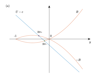
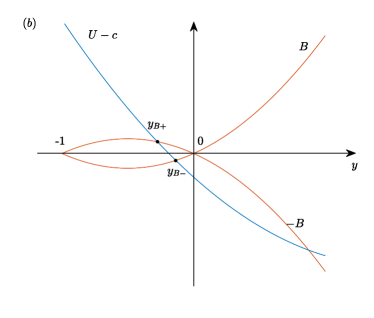
Figure 1: A sketch of the basic flow of ($a$) $U=-y$, $B=\frac{1}{2}y(y+1)$ and $(b)$ $U=-y+\frac{1}{3}y^{2}$, $B=\frac{1}{2}y(y+1)$ with two critical levels $y_{B\pm}$ for $c_{\mathrm{r}}=0.2$. There is another critical level in figure ($b$) that is not labelled.

In this section, we present typical numerical solutions of the eigenvalue problem, and give the general conclusions regarding the conditions for the instability. We use two basic flow profiles to present concrete numerical results:

$$U=-y,\quad B=\frac{1}{2}y(y+1),$$ (48)

and

$$U=-y+\frac{1}{3}y^{2},\quad B=\frac{1}{2}y(y+1).$$ (49)

It is known that the basic-flow vorticity gradient $-U^{\prime\prime}$ is responsible for hydrodynamic critical-layer instabilities. In order to exclude these instabilities and demonstrate the impact of breaking PV conservation, in the first example we use a profile that has $U^{\prime\prime}=0$ everywhere. We will show that the magnetic field itself can induce a new kind of instability. In the second example, we demonstrate how a non-zero $U^{\prime\prime}$ affects the instability. Given that the flow already has a critical-layer instability without the magnetic field (cf. Balmforth (1999)), we study how the field modifies it. A sketch of the two profiles with the critical levels identified is shown in figure 1. The field is relatively weak between $y=-1$ and $y=0$, hence the radii in the semicircle rule (25) remain positive, which retains the possibility for instability.

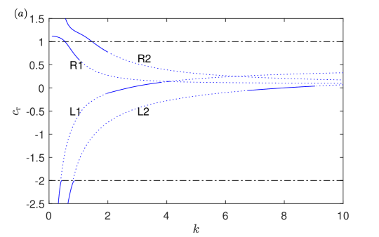
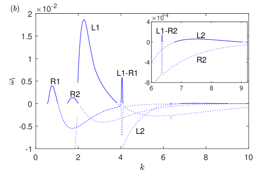
Figure 2: Numerical solution giving $c_{\mathrm{r}}$ and the unstable growth rate $\omega_{\mathrm{i}}=kc_{\mathrm{i}}$ for the basic flow profile $U=-y$, $B=\frac{1}{2}y(y+1)$ at $F=2$. Solid lines represent normal modes governed by (23) and (24), and dotted lines represent quasi-modes. ‘L1’ represents the ‘first’ mode localised near the ‘left’ boundary, and similar definitions apply for the labelling of other modes. In panel ($a$), the dash–dot lines at $c_{\mathrm{r}}=1$ and $c_{\mathrm{r}}=-2$ represent the condition that critical level $y_{B-}$ is on the boundary $y=-1$ and $y=1$, respectively.

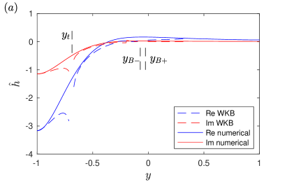
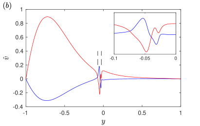
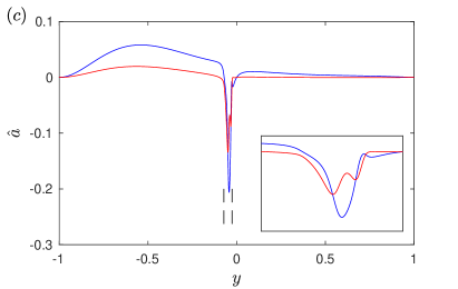
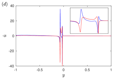
Figure 3: Eigenfunctions, $\hat{h}$, $\hat{v}$, $\hat{a}$ and $\hat{u}$ for the unstable normal mode ‘L1’ of figure 2 at $k=3$. In panel $(a)$ we have also plotted the WKB solution studied in §4, which uses the asymptotic eigenvalue and has been normalised by $\mathcal{A}=1$ in (58). The amplitude of the numerical solution is chosen by fitting to the asymptotic solution in panel $(a)$.

The numerical solutions of the dispersion relation for the basic state (48), i.e. linear $U$ and a parabolic $B$, are shown in figure 2. We plot the real part of the phase velocity $c_{\mathrm{r}}$ and the unstable growth rate $\omega_{\mathrm{i}}=kc_{\mathrm{i}}$ versus the wavenumber $k$. The solid lines represent normal mode solutions, while the dotted lines represent ‘quasi-modes’, which we will explain later in more detail. We have plotted four modes: ‘L1’ and ‘R1’ represent the first surface-gravity mode (cf. Balmforth (1999)) localised near the left and right boundary, respectively (see figure 3 for the eigenfunctions of ‘L1’). Similarly, ‘L2’ and ‘R2’ represent the second such modes. In panel 2$(a)$, the dash–dot lines $c_{\mathrm{r}}=1$ and $c_{\mathrm{r}}=-2$ are the conditions that the critical level $y_{B-}$ is on the boundary $y=-1$ and $y=1$, respectively (cf. figure 1$(a)$). In $c_{\mathrm{r}}>1$ or $c_{\mathrm{r}}<-2$, modes have no critical level and they are neutral. In the central region $-2<c_{\mathrm{r}}<1$, at least one critical level is inside the domain $-1<y<1$. It is seen that the critical levels destroy most of the normal modes, turning them into quasi-modes. On the segments of solid lines where the normal modes survive, they become unstable, as indicated by the positive growth rates in panel 2$(b)$. For ‘L1’ and ‘L2’, unstable modes appear at $c_{\mathrm{r}}\approx 0$, whereas for ‘R1’ and ‘R2’, they appear at $c_{\mathrm{r}}\approx 1$. This is related to the fact that for the profile of (48), when $c_{\mathrm{r}}=0$ or $c_{\mathrm{r}}=1$, the two critical levels coalesce at $y=0$ or $y=-1$ where $B=0$ (cf. figure 1$(a)$). These instabilities are essentially induced by the critical layers. Since $U^{\prime\prime}\equiv 0$, they are distinct from the hydrodynamic critical-layer instabilities; the local magnetic field plays the crucial role in the destabilisation, as we will elaborate subsequently. In figure 2$(b)$, we also see two narrow peaks of unstable growth rates ‘L1-R1’ and ‘L1-R2’. They are the resonant instabilities induced by two modes with nearly the same phase velocity, i.e. they correspond to the intersections of curves in figure 2$(a)$.

The eigenfunctions of $\hat{h}$, $\hat{v}$, $\hat{a}$ and $\hat{u}$ for an ‘L1’ unstable mode at $k=3$ are shown in figure 3. As stated above, the wave-like structure is localised near the left boundary $y=-1$, representing the surface-gravity mode there, and the two critical levels are close to each other near $y=0$. For $\hat{v}$, $\hat{a}$ and $\hat{u}$, there are very strong amplitude gradients in the critical layer, and because it contains two adjacent critical levels interacting with each other, the critical-layer flow is more distorted than those of hydrodynamic critical layers (see Drazin & Reid (1982) for example).

The dotted lines in figure 2 represent ‘quasi-modes’, being dotted to indicate that these ‘modes’ are not actual solutions to the eigenvalue problem, but only arise if we deform the path of $y$ into a contour in the complex plane between $y=-1$ and $y=1$. By this means, we obtain non-trivial solutions to equations (23) and (24), which are referred to as quasi-modes. Such computations usually appear when we solve an initial value problem that involves integrals in $y$, the paths of which can be deformed in the complex plane. For large times, a quasi-mode behaves like a decaying normal mode (the decay rates are shown in panel 2$(b)$), but also involves the continuous spectrum. In the early stage, however, it can contribute to transient algebraic growth under certain initial conditions (Balmforth et al., 1997). For detailed properties and behaviours of quasi-modes, see Briggs et al. (1970), Balmforth et al. (2001) and Turner & Gilbert (2007). We will briefly explain the formation of quasi-modes in our problem and our method to compute them in §4.3.

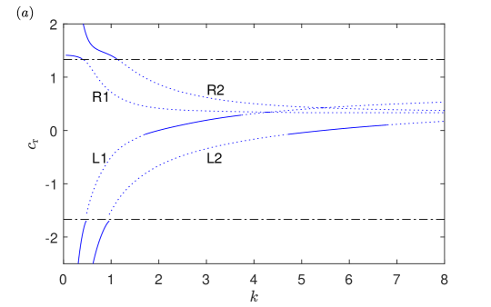
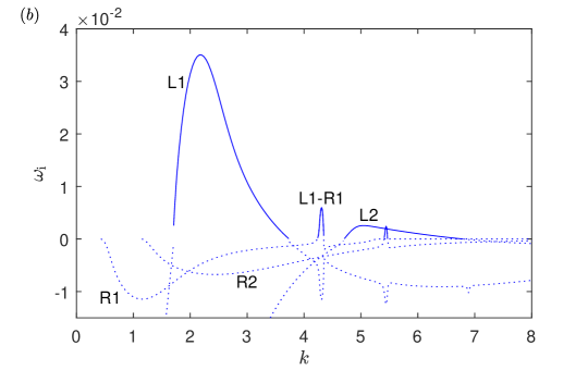
Figure 4: Numerical solution giving $c_{\mathrm{r}}$ and the unstable growth rate $\omega_{\mathrm{i}}=kc_{\mathrm{i}}$ for the basic flow profile of $U=-y+\frac{1}{3}y^{2}$, $B=\frac{1}{2}y(y+1)$ at $F=2$. Line styles and notations have the same meaning as in figure 2.

The dispersion relation for the basic state (49), i.e. parabolic profiles for both $U$ and $B$, is shown in figure 4. The general features are very similar to figure 2. The ‘L1’ and ‘L2’ unstable modes are again located where $c_{\mathrm{r}}$ is close to zero. However, we notice that there is no longer any instability of the ‘R1’ and ‘R2’ modes. In addition, the growth rates of the ‘L1’ and ‘L2’ modes have been significantly enhanced. These are essentially the effects of $U^{\prime\prime}$ in the critical layer which we will elaborate later on. Since the basic velocity profile is unstable itself, in figure 5 we plot the instability both with and without the magnetic field. The purely hydrodynamic instability (red, dashed curves) has a broader unstable waveband, since there is no additional restriction for the critical-layer instability other than the sign of $U^{\prime\prime}$ (Balmforth, 1999). Thus in the full system (blue curves) the magnetic field has the effect of narrowing the unstable waveband and also seems to inhibit the resonant instability significantly. However, the magnetic field enhances the largest growth rate of the ‘L1’ mode.

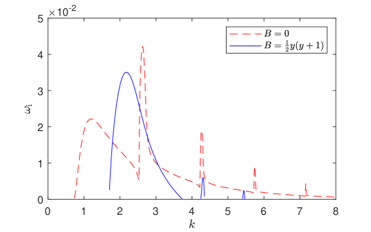
Figure 5: Growth rates of unstable ‘L1’ modes for $U=-y+\frac{1}{3}y^{2}$ with and without the magnetic field, for $F=2$.

In summary, we see that when the magnetic field is present, the critical-layer instability may only arise when the two critical levels are close to each other in one critical layer where $B\approx 0$. We will show this analytically in §4.3 using the asymptotic analysis at large $k$, and we find the closeness is described by

$$|y_{B+}-y_{B-}|\lesssim\sqrt{\frac{\pi}{k^{3}}\left|\frac{B^{\prime}B^{\prime\prime}-U^{\prime}U^{\prime\prime}}{U^{\prime 2}-B^{\prime 2}}\right|_{y=y_{B}}}\,.$$ (50)

If the two critical levels are well separated, the magnetic field is found to be stabilising and even hydrodynamic instabilities are suppressed. Note that only the two critical levels closest to the boundary where the surface-gravity mode is localised count. For example, for figure 1$(b)$, if we study the instability of the ‘L1’ and ‘L2’ modes, we only consider $y_{B+}$ and $y_{B-}$, and we do not count the additional (unlabelled) critical level further away, since disturbances are much weaker there (similarly to figure 3). Also note that the two critical levels must come from each of $U-c-B=0$ and $U-c+B=0$; if both of them belong to $U-c-B=0$ (or both to $U-c+B=0$), the critical levels still have a stabilising effect even if they are close to each other.

Our asymptotic analysis also indicates that once the two critical levels are close, the key quantity that determines the instability is $B^{\prime}B^{\prime\prime}-U^{\prime}U^{\prime\prime}$ in the critical layer. In particular, for modes localised near the left boundary (i.e. ‘L1’, ‘L2’ etc.), the condition for instability is that in the critical layer,

$$B^{\prime}B^{\prime\prime}-U^{\prime}U^{\prime\prime}>0.$$ (51)

By performing a rotation of the domain, the condition for the instability of the modes localised near the right boundary is that in the critical layer,

$$B^{\prime}B^{\prime\prime}-U^{\prime}U^{\prime\prime}<0.$$ (52)

These conditions are generalisations of hydrodynamic critical-layer instabilities based on the vorticity gradient $-U^{\prime\prime}$ (Balmforth, 1999; Riedinger & Gilbert, 2014), and they can well explain the numerical results we just presented. For the profile of (48), $B^{\prime}B^{\prime\prime}-U^{\prime}U^{\prime\prime}=\frac{1}{2}$ at $y=0$, so (51) is satisfied and ‘L1’ and ‘L2’ are destabilised when the critical levels are near $y=0$. Similarly, $B^{\prime}B^{\prime\prime}-U^{\prime}U^{\prime\prime}=-\frac{1}{2}$ at $y=-1$, so (52) is satisfied, and ‘R1’ and ‘R2’ are destabilised when the critical levels are near $y=-1$. Since $U^{\prime\prime}=0$ for this profile, it is the magnetic field that plays the key role in the destabilisation via the current gradient $J^{\prime}=-B^{\prime\prime}$. When we include curvature of $U$, in the profile (49), $B^{\prime}B^{\prime\prime}-U^{\prime}U^{\prime\prime}=\frac{7}{6}$ at $y=0$, so unstable modes ‘L1’ and ‘L2’ again exist, but $B^{\prime}B^{\prime\prime}-U^{\prime}U^{\prime\prime}=\frac{11}{18}$ at $y=-1$ which violates (52), and so instability of the modes of ‘R1’ and ‘R2’ no longer occurs, as shown in figure 4. Once the condition (51) or (52) is satisfied, the largest growth rate increases with the value of $|B^{\prime}B^{\prime\prime}-U^{\prime}U^{\prime\prime}|$ in the critical layer if the unstable wavenumbers remain similar, as we see in figures 2, 4 and 5 for the ‘L1’ modes. We note that our asymptotic analysis is based on large $k$, but we find that for the conditions we study, it still gives qualitatively good results even when $k$ is of the order of unity.

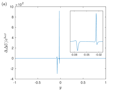
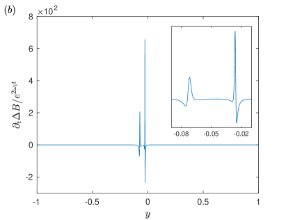
Figure 6: Mean-flow acceleration of (a) streamwise velocity and (b) magnetic field corresponding to the unstable mode of figure 3.

The numerical results for $\partial_{t}\Delta U$ and $\partial_{t}\Delta B$ from (44) and (46) for the unstable mode of figure 3 are plotted in figure 6, normalised by the exponential growth $\exp(2\omega_{\mathrm{i}}t)$. The mean-flow responses are strongly localised around the two critical levels. The flow response $\Delta U$ generally exhibits two jets forced in opposite directions. The profile of $\Delta B$ is a little different: it is extended in both directions at each critical level, which may be understood as a result of stretching caused by the mean-flow jet, following Alfvén’s theorem.

Another prominent feature of figure 6 is that there is almost no mean-flow or mean-field response outside the critical layer: we find that the amplitudes of both are of magnitude $0.01$ or smaller. In non-magnetic hydrodynamic mean-flow theory, $\partial_{t}\Delta U\approx 0$ outside the critical layer may be inferred from the ‘non-acceleration rule’ (which also applies when the PV is not zero). This rule states that the mean-flow velocity is not accelerated if the waves are steady and there is no dissipation (see Bühler, 2014). Apparently, adding a streamwise magnetic field does not change this in our problem. In appendix B, we give a mathematical proof that $\partial_{t}\Delta U$ and $\partial_{t}\Delta B$ are both zero outside the critical layer in the limit of neutral stability, hence the use of analytical continuation implies $\partial_{t}\Delta U$ and $\partial_{t}\Delta B$ are of order $\omega_{\mathrm{i}}$, which is small. We note that in hydrodynamic wave–mean flow interaction, the derivation of the non-acceleration rule strongly depends on PV conservation, so it is a little surprising that it still holds when the magnetic field breaks this conservation. Our mathematical derivation in appendix B shows that in each of the quadratic terms of (44–46), if the wave is steady, i.e. $c_{\mathrm{i}}=0$, then the two components of linear waves have a phase difference of $\pi/2$, hence their product is still a wave with zero mean value. We do not have a deeper physical explanation at present, nor can we extend this conclusion to more general flows.

The momentum conservation represented by equation (40) can provide an explanation for the mechanism of the instability. As we see in figure 6, the mean-velocity acceleration $\partial_{t}\Delta U$ is very strong in the critical layer. We can show that its integral in $y$ over the critical layer has a non-trivial value, which represents a source of mean momentum $M_{\mathrm{m}}$. Thus, it drives the exponential growth of the outer flow following the conservation of momentum. We will demonstrate details of this mechanism in §4.4, taking advantage of the large-wavenumber asymptotics.

4 The asymptotic analysis

In order to better understand the instability and obtain conclusions for general smooth profiles, we perform an asymptotic analysis at large wavenumbers. This allows us to derive the instability criteria exhibited in §3 analytically. We will combine WKB solutions through the bulk of the flow and a local analysis near the critical levels, highlighting the effects of the singularities, and then derive an asymptotic solution for the eigenvalue $c$. The methodology is similar to Riedinger & Gilbert’s (2014) analysis of shallow water instability and Wang & Balmforth’s (2018) analysis of strato-rotational instability, but here we have a more complicated critical layer since there are two critical levels inside. We will also study the conservation law of momentum in detail to provide a mechanism for the instability. We will only study the instability induced by critical layers as the principal goal of this paper, though we note that critical layers may also affect the resonant instability, a topic we leave for further research.

4.1 WKB solutions

We rewrite equation (23) as

$$\hat{h}^{\prime\prime}-\frac{[(U-c)^{2}-B^{2}]^{\prime}}{(U-c)^{2}-B^{2}}\,\hat{h}^{\prime}+l^{2}\hat{h}=0,$$ (53)

where

$$l^{2}=-\lambda^{2}=-k^{2}\left\{1-F^{2}[(U-c)^{2}-B^{2}]\right\}.$$ (54)

In the short-wavelength limit $k\gg 1$, $l,\lambda\gg 1$, thus (53) has WKB solutions. Since $c_{\mathrm{i}}$ is a small number, we may assume $c\approx c_{\mathrm{r}}$ in (53) and (54), and hence $l^{2}$ and $\lambda^{2}$ are approximately real, as long as we are not close to the critical levels. The height field $\hat{h}$ is wavelike when $l^{2}>0$ and evanescent when $\lambda^{2}>0$; $l$ and $\lambda$ represent the approximate wavenumber and the exponential decay rate, respectively.

We take the modes localised near the left boundary, i.e. ‘L1’ and ‘L2’ in figure 2, as an example for the asymptotic analysis. The distribution of $l^{2}$ for the eigenfunction of figure 3 is shown in figure 7. There is a turning point located at $y=y_{\mathrm{t}}$ where $l^{2}=0$. Hence $\hat{h}$ is wavelike in $-1<y<y_{\mathrm{t}}$ and evanescent in $y>y_{t}$, which can also be seen in figure 3. The two critical levels $y_{B\pm}$ are in the evanescent region. They render a thin critical layer where the WKB solution fails. For convenience, we define their midpoint as

$$y_{B}=\frac{y_{B+}+y_{B-}}{2}\,,$$ (55)

representing the centre of the critical layer.

For general basic flow profiles, it is also necessary for the instability that $l^{2}>0$ near the boundary, so that $\hat{h}$ is wavelike and the surface-gravity mode can exist. For modes localised near the left boundary, this means

$$U-c>\sqrt{B^{2}+F^{-2}}\quad\mathrm{or}\quad U-c<-\sqrt{B^{2}+F^{-2}}\quad\mathrm{at}\quad y=-1.$$

It is also necessary that there is no other critical level other than $y_{B\pm}$ between $y_{B}$ and $y=-1$ (otherwise that critical level would be the dominant one to determine the instability property and hence the subject to study). The continuous functions $U(y)-c\pm B(y)$ have designated signs at $y=-1$ indicated by ($(56a,b)$), but are nearly zero at $y=y_{B}$, hence to guarantee they have no other zeros in between, the signs of their derivatives at $y=y_{B}$ are also fixed, that is,

$$U^{\prime}\pm B^{\prime}<0\quad\mathrm{or}\quad U^{\prime}\pm B^{\prime}>0\quad\mathrm{at}\quad y=\operatorname{\mathrm{Re}}y_{B},$$

corresponding to ($(56a,b)$$a$) and ($(56a,b)$$b$), respectively. Whether the critical layer has ($(57a,b)$$a$) or ($(57a,b)$$b$) holding will determine the sign of $\operatorname{\mathrm{Im}}y_{B\pm}$ (see (28)), and therefore results in a similar derivation with numerous sign changes. We will use the combination of ($(56a,b)$$a$) and ($(57a,b)$$a$) for our derivation, which is the case for figure 1. The other situation of ($(56a,b)$$b$) and ($(57a,b)$$b$) will be noted briefly, and in fact, the resulting condition for instability is the same. The flow field in $y>y_{B}$ is not important since the disturbance is weak there. There could be other turning points or critical levels in $y>y_{B}$, as long as they are not close to $y_{B}$.

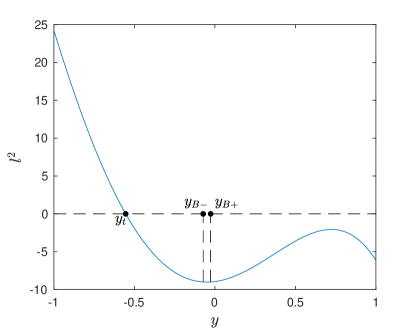
Figure 7: Distribution of $l^{2}$ for the mode of figure 3.

In $y>y_{B}$, we consider the WKB solution of (53) that decays exponentially:

$$\hat{h}=\mathcal{A}\,\sqrt{\frac{(U-c)^{2}-B^{2}}{\lambda}}\,\exp\biggl{(}-\int_{y_{B}}^{y}\lambda(y^{\prime})\,\mathrm{d}y^{\prime}\biggr{)},$$ (58)

where $\mathcal{A}$ is an arbitrary constant. In $y_{\mathrm{t}}<y<y_{B}$, because of the critical layer, both exponential solutions exist, and $\hat{h}$ is expressed by

$$\hat{h}=\mathcal{A}_{-}\hat{h}_{-}+\mathcal{A}_{+}\hat{h}_{+},$$ (59)

where $\mathcal{A}_{-}$ and $\mathcal{A}_{+}$ are constants and $\hat{h}_{-}$ and $\hat{h}_{+}$ are the exponentially decaying and growing solutions, respectively:

$$\hat{h}_{\pm}=\sqrt{\frac{(U-c)^{2}-B^{2}}{\lambda}}\,\exp\biggl{(}\pm\int_{y_{B}}^{y}\lambda(y^{\prime})\,\mathrm{d}y^{\prime}\biggr{)}.$$ (60)

In $-1<y<y_{\mathrm{t}}$, (59) is still applicable but we need to find the corresponding wavelike solutions of $\hat{h}_{-}$ and $\hat{h}_{+}$. Following the standard procedure to match across the turning point $y_{\mathrm{t}}$ via Airy functions (cf. Bender & Orszag, 2013; Hinch, 1991), we find

$$\hat{h}_{-}=2\,\sqrt{\frac{(U-c)^{2}-B^{2}}{l}}\,\Psi\,\cos\biggl{[}\int_{y_{t-}}^{y}l(y^{\prime})\,\mathrm{d}y^{\prime}+\frac{\pi}{4}\biggr{]},$$

$$\hat{h}_{+}=\sqrt{\frac{(U-c)^{2}-B^{2}}{l}}\,\frac{1}{\Psi}\,\cos\biggl{[}\int_{y_{t-}}^{y}l(y^{\prime})\,\mathrm{d}y^{\prime}-\frac{\pi}{4}\biggr{]},$$

where

$$\Psi=\exp\left(\int_{y_{\mathrm{t}}}^{y_{B}}\lambda\,\mathrm{d}y\right)$$ (62)

represents the exponential gain (loss) of the amplitude of $\hat{h}_{-}$ ($\hat{h}_{+}$) from $y_{B}$ to $y_{\mathrm{t}}$. We will need to determine the relation between $\mathcal{A}$, $\mathcal{A}_{-}$ and $\mathcal{A}_{+}$ through analysis of the critical layer which connects (58) and (59).

4.2 Local solution in the critical layer

In the critical layer, we introduce a stretched coordinate

$$\eta=\frac{y-y_{B}}{\delta}\,,\quad\delta=k^{-1}\ll 1,$$ (63)

based on the short-wave limit. To derive a local equation for (23), we Taylor expand $U-c\pm B$ around their zeros $y_{B\pm}$, then substitute in the local coordinate (63) and take the leading two orders of $\delta$. After some algebra, we arrive at the local equation

$$\hat{h}_{\eta\eta}+\left(\gamma-\frac{2\eta}{\eta^{2}-D^{2}}\right)\hat{h}_{\eta}-\hat{h}=0,$$ (64)

with two parameters

$$D=\frac{y_{B+}-y_{B-}}{2\delta}\,,\quad\gamma=-\delta\,\frac{B^{\prime}B^{\prime\prime}-U^{\prime}U^{\prime\prime}}{B^{\prime 2}-U^{\prime 2}}\,\bigg{|}_{y=y_{B}}.$$

The quantity $D$ represents a rescaled distance between the two critical levels which are located at $\eta=\pm D$ in the local equation, hence we refer to $D$ as the ‘separation parameter’. The parameter $\gamma$ is determined by the curvature of the profiles of the basic velocity and magnetic field, and is therefore referred to as the ‘curvature parameter’. When the magnetic field vanishes, the separation parameter $D=0$ and we recover the hydrodynamic critical level at $\eta=0$, with the curvature parameter $\gamma$ determined by the vorticity gradient $Q^{\prime}=-U^{\prime\prime}$. When a magnetic field is involved, the current gradient $J^{\prime}=-B^{\prime\prime}$ appears on an equal footing. It should be noted that although the curvature parameter $\gamma=O(\delta)$ is algebraically small, it plays a crucial role in the singularity and instability. This can be easily understood for the hydrodynamic case $D=0$: $\gamma$ determines the strength of the singularity at $\eta=0$, and the singularity becomes removable if $\gamma$ is absent. Similar arguments have also been given by Riedinger & Gilbert (2014).

To provide the connection condition for the outer WKB solution, we consider the behaviour of $\hat{h}(\eta)$ in an intermediate regime $y-y_{B}=O(\delta^{\frac{1}{2}})$, or $\eta=O(\delta^{-\frac{1}{2}})$. Applying the method of dominant balance (Bender & Orszag, 2013) to (64), we find

$$\hat{h}\sim\left\{\begin{array}[]{ll}\alpha\eta e^{-\eta},&\eta=O(\delta^{-\frac{1}{2}}),\;\eta>0,\\ \alpha_{-}(-\eta)e^{-\eta}+\alpha_{+}(-\eta)e^{\eta},&\eta=O(\delta^{-\frac{1}{2}}),\;\eta<0,\end{array}\right.$$

where $\alpha$, $\alpha_{-}$ and $\alpha_{+}$ are constants. For positive $\eta$, only the decaying solution is included in accordance with the WKB solution. We will see that the key quantity that controls the instability is

$$\beta=\Imag\left(\frac{\alpha_{+}}{\alpha_{-}}\right),$$ (67)

representing the phase difference between the growing and decaying amplitude for negative $\eta$, and we will study its properties in detail. The relation between $\alpha_{-}$ and $\alpha$, representing the amplitudes on two sides of the critical layer, is noted in appendix A.

When $D=0$, i.e. two critical levels overlap exactly, $\hat{h}$ can be represented by confluent hypergeometric functions, and we can derive the analytical connection condition. We can show that under the condition of ($(57a,b)$$a$) and $c_{\mathrm{i}}\rightarrow 0^{+}$, in the limit of small $\gamma=O(\delta)$,

$$\beta|_{D=0}=\frac{\pi}{2}\,\gamma.$$ (68)

This result has been derived by Riedinger & Gilbert (2014) for hydrodynamic shallow water critical layers, but continues to apply when we include the field curvature in $\gamma$. Note that (68) is the leading-order solution for small $\gamma$; a more precise solution for finite $\gamma$ is given in ($(97a,b,c)$$c$) in appendix A. When $D\neq 0$, we have not been able to derive the connection formula analytically. Equation (64) may be converted to Heun’s equation (cf. Arscott et al., 1995), but still, we have not been able to find analytical connection formulae for Heun’s functions in the literature. Therefore, we will resort to numerical solutions of (64).

There are some issues to which we should pay attention when solving the equation numerically. First, we need to make sure that we select the correct branch when passing the logarithmic branch points. The Frobenius solutions of (64) around $\eta=\mp D$ are

$$\hat{h}=C_{s\pm}\Bigl{[}1+\tfrac{1}{2}(\eta\pm D)^{2}\log(\eta\pm D)+\cdots\Bigr{]}+C_{r\pm}\left[\frac{(\eta\pm D)^{2}}{k^{2}}+\cdots\right],$$ (69)

which are equivalent to (27). By definition, $y_{B\pm}$, $\eta$, $D$ and $\gamma$ are all slightly complex due the small growth rate $c_{\mathrm{i}}$. Our aim is to approach the limit $c_{\mathrm{i}}\rightarrow 0^{+}$ if numerically possible, so as to draw parallel conclusions with the analytical relation (68). But we also need to make sure that in (69) we select the same branch as (27) for the logarithm function, and therefore, we require that $\Imag(\eta\pm D)$ and $\Imag(y-y_{B\pm})$ have the same sign. According to equation (28), the quantities $\operatorname{\mathrm{Im}}y_{B\pm}$ are negative for an unstable mode if we prescribe the condition ($(57a,b)$$a$). So for convenience, we assume $D$ and $\gamma$ to be real but add a very small $positive$ imaginary part to $\eta$ when integrating (64) numerically. In practice, we use $\operatorname{\mathrm{Im}}\eta=10^{-6}$–$10^{-8}$; using different values of $\operatorname{\mathrm{Im}}\eta$ in this range does not affect the solution for $\hat{h}$ or $\beta$.

There is also a technical issue regarding the large $|\eta|$ limits. The asymptotic behaviour ($(66a,b)$) becomes precise when $|\eta|$ is very large, but numerically, $\alpha_{+}(-\eta)e^{\eta}$ becomes too small compared to $\alpha_{-}(-\eta)e^{-\eta}$ for very large $-\eta$, and the value of the former may not be precisely stored in $\hat{h}$ within the usual numerical precision. To tackle this difficulty, we develop a numerical method that separately computes the solution corresponding to the limit of $\alpha_{+}(-\eta)e^{\eta}$, based on shooting from both sides of the domain. Details of this method are presented in appendix A.

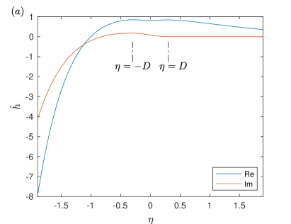
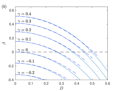
Figure 8: ($a$) The local solution of $\hat{h}$ at $D=0.3$, $\gamma=0.3$, and $(b)$ $\beta$ as a function of $D$ and $\gamma$ for the condition ($(57a,b)$$a$). In panel $(b)$, solid lines represent the numerical solution for $\beta$, and dashed lines show the results of the empirical fitting (70)

.

A sample solution for $\hat{h}$ is given in figure 8($a$): $\hat{h}$ in general decays exponentially, but becomes flat at the two critical levels, as predicted by the Frobenius solution (69). There is a phase shift of the decaying amplitude across the critical layer, which is rendered by a complex $\alpha_{-}/\alpha$. The numerical solution for the key quantity $\beta$ is shown in figure 8$(b)$ in solid curves, as a function of the separation parameter $D$ and the curvature parameter $\gamma$. It is clearly seen that $\beta$ increases with $\gamma$ but decreases with $D$. In our subsequent analysis, we are concerned about the situation where $\beta$ is positive, as this is the condition that instability may arise. When the two critical levels overlap, i.e. $D=0$, our analytical solution (68) indicates that the curvature parameter $\gamma$ has to be positive for $\beta$ to be positive, which is also seen in the figure. When $D\neq 0$, we found that the decrease of $\beta$ with $D$ can be well fitted by a quadratic function

$$\beta\approx\beta\,|_{D=0}-2D^{2}.$$ (70)

The results of (70) are plotted in figure 8$(b)$ in dashed lines. Hence a positive $\beta$ requires $|D|$ to be relatively small. According to the value of $\beta\,|_{D=0}$ provided by (68), we need $|D|\lesssim\sqrt{\pi\gamma}/2$.

4.3 Matching and eigenvalues

We take the limit of $y\rightarrow y_{B}$ for the WKB solutions (58) and (59), and then match them to the inner solution ($(66a,b)$). This provides the connection conditions

$$\frac{\mathcal{A}}{\alpha}=\sqrt{\frac{k^{3}}{U_{B}^{\prime 2}-B_{B}^{\prime 2}}}\,,\quad\frac{\mathcal{A}_{-}}{\mathcal{A}}=\frac{\alpha_{-}}{\alpha},\quad\frac{\mathcal{A}_{+}}{\mathcal{A}-}=\frac{\alpha_{+}}{\alpha_{-}}\,,\quad\Imag\left(\frac{\mathcal{A}_{+}}{\mathcal{A}_{-}}\right)=\beta.$$ (71)

Finally, we incorporate the boundary conditions to determine the eigenvalue $c$. For modes localised near the left boundary, the eigenfunction $\hat{h}$ has an exponential decay structure, so its amplitude is much larger near the left boundary $y=-1$ than near the right boundary $y=1$. Therefore, the eigenvalue is primarily determined by the boundary condition at $y=-1$, namely $\hat{h}^{\prime}(-1)=0$, which is

$$\hat{h}_{-}^{\prime}(-1)+\frac{\mathcal{A}_{+}}{\mathcal{A}_{-}}\,\hat{h}_{+}^{\prime}(-1)=0.$$ (72)

Since $|\hat{h}_{-}|\gg|\hat{h}_{+}|$ given $\Psi\gg 1$, the dominant balance of (72) is

$$\hat{h}^{\prime}_{-}(-1)=0.$$ (73)

Substituting in ($(61a)$$a$) and taking the leading order in terms of $l\gg 1$, we can derive an integral dispersion relation

$$\int_{-1}^{y_{t}}l(y^{\prime},c_{\mathrm{r}})\,\mathrm{d}y^{\prime}=\left(n\pi-\frac{3}{4}\pi\right),\quad n=1,2,\ldots.$$ (74)

Equation (74) implicitly determines $c=c_{\mathrm{r}}$ which is real. In absence of a critical layer, it determines the phase velocity of a neutral surface-gravity mode in the large wavenumber limit. The integer $n$ represents the index of the mode, i.e. L1 and L2 in figure 2 correspond to $n=1$ and $n=2$.

The exponentially small $\hat{h}_{+}$ in (72), however, can make $c$ complex and render an unstable flow. Suppose including the $\hat{h}_{+}$ term causes a small correction to the phase velocity: $c_{\mathrm{r}}\rightarrow c_{\mathrm{r}}+\Delta c$, then from (72) and (73), we have

$$\frac{\partial}{\partial c}\,\hat{h}_{-}^{\prime}(-1)\Big{|}_{c=c_{\mathrm{r}}}\Delta c+\frac{\mathcal{A}_{+}}{\mathcal{A}_{-}}\,\hat{h}^{\prime}_{+}(-1)\Big{|}_{c=c_{\mathrm{r}}}=0.$$ (75)

It is now apparent that $\Imag(\mathcal{A}_{+}/\mathcal{A}_{-})=\beta$ can generate an imaginary part $c_{\mathrm{i}}$ of $\Delta c$, which demonstrates how the critical layer can make the flow unstable. Substituting ($(61a)$) into (75), again taking the leading order of $l$, after some algebra we find

$$c_{\mathrm{i}}=-\frac{\beta}{2\Psi^{2}\displaystyle\int_{-1}^{y_{\mathrm{t}}}\left(\displaystyle\frac{\partial l}{\partial c}\right)_{c=c_{\mathrm{r}}}\mathrm{d}y}\,,\qquad\frac{\partial l}{\partial c}=-\frac{kF^{2}(U-c)}{\sqrt{F^{2}[(U-c)^{2}-B^{2}]-1}}\,.$$ (76)

As prescribed in ($(56a,b)$$a$), $U>c_{\mathrm{r}}$ near the left boundary $y=-1$, and so an unstable mode $c_{\mathrm{i}}>0$ requires $\beta>0$. The WKB solution for $\hat{h}$ is compared with the numerical solution in figure 3$(a)$. The asymptotic solutions of $c_{\mathrm{r}}$ and $c_{\mathrm{i}}$ for the dispersion relation of figure 4 are plotted in figure 9. For both ‘L1’ and L2’ mode, the asymptotic solution becomes inaccurate for smaller $k$, because for negative $c_{\mathrm{r}}$, the additional critical level in figure 1$(b)$ moves close to $y_{B\pm}$, and all critical levels may disappear. These effects are not included in the asymptotic analysis, and make the error of $c_{\mathrm{i}}$ very sensitive to the error of $c_{\mathrm{r}}$. But overall, the asymptotic analysis for $k\gg 1$ gives qualitatively good predictions to the eigenfunction and the eigenvalue, and in fact, it still works well when $k$ is of the order of unity as we see in figure 9.

Hence the crucial condition that the critical layer destabilises the mode localised near the left boundary is $\beta>0$, for the situation under the conditions ($(56a,b)$$a$) and ($(57a,b)$$a$). As shown in figure 8, a positive $\beta$ requires two conditions: the curvature parameter $\gamma$ should be positive and the separation parameter $D$ should be relatively small. The first condition requires that the curvature of the profiles of the basic velocity and field have designated signs in the critical layer, that is

$$B^{\prime}B^{\prime\prime}-U^{\prime}U^{\prime\prime}>0\quad\mathrm{at}\quad y=y_{B},$$ (77)

The second condition, on the other hand, requires that the two critical levels should be close to each other:

$$|y_{B+}-y_{B-}|\lesssim\frac{\sqrt{\pi\gamma}}{k}$$ (78)

approximately from (70). It is straightforward to check that for the case of fields satisfying ($(56a,b)$$b$) and ($(57a,b)$$b$), the condition for the critical layer to destabilise the mode near the left boundary is the same. We only need to pay attention to the fact that in this case $U-c_{\mathrm{r}}<0$ in (76) but we replace $\beta$ by $-\beta$ in (68) and figure 8$(b)$, a consequence of the sign of $\operatorname{\mathrm{Im}}y_{B\pm}$ reversing (see (28). From equations ($(65a,b)$$b$, 68, 70, 76), we also see that the maximum value of the growth rate is proportional to $\gamma$ if the other quantities in (76) remain similar, and thus the growth rate is positively correlated with the value of $B^{\prime}B^{\prime\prime}-U^{\prime}U^{\prime\prime}$ in the critical layer. The conditions and properties of the instability exhibited in §3 are therefore derived analytically.

If $c_{\mathrm{i}}$ predicted by (76) becomes negative, it does not represent a decaying normal mode. This is because $c_{\mathrm{i}}<0$ implies $\operatorname{\mathrm{Im}}\eta<0$, which is inconsistent with our choice of $\operatorname{\mathrm{Im}}\eta\rightarrow 0^{+}$ in the critical layer based on the prescription of $c_{\mathrm{i}}>0$ (cf. (28, 63, 69) and related discussion). In such situations, the normal mode cannot exist: it is destroyed by the critical layer. In the setting of an initial value problem, however, the solution of the Laplace-transformed variable involves integrals in $y$, and one may deform the integral contour in the complex plane (Briggs et al., 1970). If we choose $\operatorname{\mathrm{Im}}y>\operatorname{\mathrm{Im}}y_{B\pm}>0$ on the contour, then $\operatorname{\mathrm{Im}}\eta$ is still positive even when $c_{\mathrm{i}}<0$. In this way, we may recover the solution to the eigenvalue problem (23, 24) for complex $y$, which is the quasi-mode we referred to earlier in §3. For the numerical solution of the quasi-modes shown in figures 2 and 4, we have applied the shooting method on the complex contour:

$$y=w+\mathrm{i}\alpha(1-w^{2}),\quad-1<w<1,\quad\alpha>0,\quad\alpha,w\;\mathrm{real},$$ (79)

which is an arc connecting $y=-1$ and $y=1$ in the complex plane with $\operatorname{\mathrm{Im}}y>0$. For the theoretical foundations of recovering quasi-modes from initial value problems, see Briggs et al. (1970).

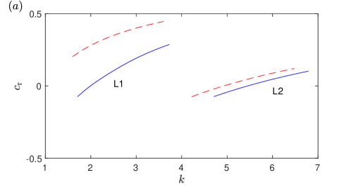
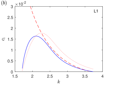
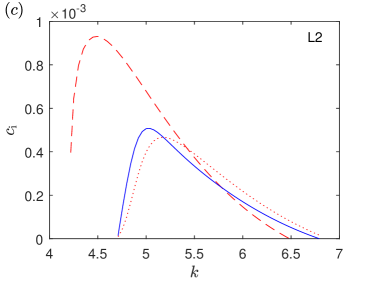
Figure 9: Comparison between the numerical solution (solid lines) and asymptotic solution (dashed lines) for $c_{\mathrm{r}}$ and $c_{\mathrm{i}}$ for the dispersion relation in figure 4. Dotted lines for $c_{\mathrm{i}}$ are the solutions predicted by momentum conservation in (89).

4.4 Implications of momentum conservation

Finally, we study the momentum conservation in (40) to provide a mechanism for the critical-layer instability in this system. In studies of hydrodynamic instabilities, the conservation law has been used to represent the signature of different types of instabilities. For example, Rayleigh’s instability features the conservation of mean momentum $M_{\mathrm{m}}$ (Bühler, 2014); the resonance instability of shallow-water flows with linear shear velocities features the cancellation of wave momentum $M_{\mathrm{w}}$ with opposite signs (Balmforth et al., 1997), and the critical-layer instability of shallow-water flows features a balance between the wave momentum $M_{\mathrm{w}}$ and the mean momentum $M_{\mathrm{m}}$ (Balmforth et al., 1997; Riedinger & Gilbert, 2014).

The wave momentum is determined by the global structure of the unstable mode:

$$M_{\mathrm{w}}=2\hat{M}_{\mathrm{w}}\,e^{2\omega_{\mathrm{i}}t},\quad\hat{M}_{\mathrm{w}}=\int_{-1}^{1}\tfrac{1}{2}(\hat{h}\hat{u}^{*}+\hat{u}\hat{h}^{*})\,\mathrm{d}y.$$ (80)

Although $\hat{u}$ is locally strong in the critical layer, because the critical layer is too thin, $\hat{h}\hat{u}^{*}+\hat{u}\hat{h}^{*}$ is still not strong enough to give a significant contribution to the integral from the critical layer. Outside the critical layer, the exponential decay of the eigenfunctions implies that the main contribution to the integral comes from the region $y\in[-1,y_{\mathrm{t}}]$. Hence in the large-$k$ limit, using (22) and $(\ref{18})$, one can derive that

$$\hat{M}_{\mathrm{w}}\simeq-\int_{-1}^{y_{\mathrm{t}}}\frac{U-c_{\mathrm{r}}}{F^{2}[(U-c_{\mathrm{r}})^{2}-B^{2}]}\,|\hat{h}|^{2}\,\mathrm{d}y.$$ (81)

Given conditions ($(56a,b)$$a$) and ($(57a,b)$$a$), $\hat{M}_{\mathrm{w}}<0$, and hence for an unstable mode,

$$\frac{\mathrm{d}M_{\mathrm{w}}}{\mathrm{d}t}=4\omega_{\mathrm{i}}\hat{M}_{\mathrm{w}}\,e^{2\omega_{\mathrm{i}}t}<0.$$ (82)

For the mean-flow momentum, we have found that the value of $\partial_{t}\Delta U$ is at $O(k^{-1}\omega_{\mathrm{i}}|\hat{v}|^{2})$ outside the critical layer, which is $O(k^{-1})$ smaller compared to the wave momentum in the large-$k$ limit. Details of the computation are given in appendix B. Hence it is the critical-layer mean-flow acceleration that balances the wave momentum, which is the same as for hydrodynamic shallow-water instabilities (Balmforth et al., 1997; Riedinger & Gilbert, 2014). Let $\Delta$ be half of the critical-layer thickness, then we choose $\Delta=O(\delta^{\frac{1}{2}})$ as we did in ($(66a,b)$). Substituting (44, 31, 11) into (47), we derive

$$\frac{\mathrm{d}M_{\mathrm{m}}}{\mathrm{d}t} \simeq\int_{y_{B}-\Delta}^{y_{B}+\Delta}\frac{\partial\Delta U}{\partial t}\,\mathrm{d}y$$

$$=\int_{y_{B}-\Delta}^{y_{B}+\Delta}\left[-\overline{(uv)_{y}}+\overline{U^{\prime}vh-u(h_{t}+Uh_{x})}-\overline{(a_{x}a_{y})_{y}}+\overline{a_{x}(Bh_{y}+2B^{\prime}h)}\right]\,\mathrm{d}y.$$ (83)

From the Frobenius solutions (27) or (2.2), together with the relation (22), one can show that the dominant terms of (83) are $-\overline{(vu)_{y}}$ and $-\overline{(a_{x}a_{y})_{y}}$, and other terms which involve the surface displacement $h$ are much smaller. Therefore,

$$\frac{\mathrm{d}M_{\mathrm{m}}}{\mathrm{d}t}\simeq-\left.\overline{(uv+a_{x}a_{y})}\right.\Big{|}_{y_{B}-\Delta}^{y_{B}+\Delta}.$$ (84)

Equation (84) indicates the mean-flow response is determined by the jump of Reynolds stress $\overline{uv}$ and Maxwell stress $\overline{a_{x}a_{y}}$ across the critical layer, and it extends the result of the mean-flow response of hydrodynamic critical layers determined by the jump of the Reynolds stress (for example, Killworth & McIntyre, 1985; Booker & Bretherton, 1967). At the edge of the critical layer $y_{B}\pm\Delta$, using (22) with $\delta\ll\Delta\ll 1$, we can show the following relation holds:

$$\overline{a_{x}a_{y}}\simeq-\left(\frac{B_{B}^{\prime}}{U_{B}^{\prime}}\right)^{2}\overline{uv}.$$ (85)

So the Maxwell stress has the opposite sign to the Reynolds stress, similar to what was found by Gilman & Fox (1997), and given $|B^{\prime}_{B}|<|U^{\prime}_{B}|$ in our problem (see ($(57a,b)$$a$)), the former is weaker. We note that we should not interpret the Maxwell stress as the overall effect of the magnetic field, because the Reynolds stress is also controlled by the value of $B^{\prime}B^{\prime\prime}-U^{\prime}U^{\prime\prime}$ in the critical layer.

To find the value of $\mathrm{d}_{t}M_{\mathrm{m}}$, we first substitute the normal mode solution (16, 22) into (84) to represent it in terms of $\hat{h}$: in the limit of large $k$,

$$\frac{\mathrm{d}M_{\mathrm{m}}}{\mathrm{d}t}\simeq e^{2\omega_{\mathrm{i}}t}\left.\left[\frac{2\,\Imag(\hat{h}^{{}^{\prime}*}\hat{h}^{\prime\prime})}{k^{3}F^{4}|(U-c)^{2}-B^{2}|}\right]\right|_{y_{B}-\Delta}^{y_{B}+\Delta}.$$ (86)

Then we use the asymptotic solution ($(66a,b)$) to compute the value of $\hat{h}$ at $y_{B}\pm\Delta$. Using the property that $D\delta\ll\Delta\ll 1$ and the relations in (71), after some algebra, we derive a compact result in terms of $\beta$

$$\frac{\mathrm{d}M_{\mathrm{m}}}{\mathrm{d}t}\simeq 4e^{2\omega_{\mathrm{i}}t}\,\frac{|\mathcal{A}_{-}|^{2}\beta}{kF^{4}}\,.$$ (87)

When the magnetic field is switched off, from (22$b$, 68, 71, $(97a,b,c)$$b$), together with $\hat{h}|_{\eta=0}=\alpha$ for the local solution, a property of the relevant confluent hypergeometric function, it can shown that (87) reduces to

$$\frac{\mathrm{d}M_{\mathrm{m}}}{\mathrm{d}t}\simeq e^{2\omega_{\mathrm{i}}t}\,\frac{2\pi|\hat{v}_{c}|^{2}U_{c}^{\prime\prime}}{k|U_{c}^{\prime}|}\,,$$ (88)

where now we use the subscript $c$ to represent the hydrodynamic critical level $y_{c}$. Equation (88) is the classical result for the mean-flow momentum forced in the critical layer (Miles, 1957; Vekstein, 1998; Balmforth, 1999; Riedinger & Gilbert, 2014), with the important implication that its value is proportional to the local vorticity gradient $-U_{c}^{\prime\prime}$. So again, we have generalised this result to MHD flows through use of the phase difference parameter $\beta$. To balance $\mathrm{d}_{t}M_{\mathrm{w}}<0$, (87) should be positive, which again requires $\beta>0$. The balance between (82) and (87) yields another expression for $c_{\mathrm{i}}$,

$$c_{\mathrm{i}}=-\frac{|\mathcal{A}_{-}|^{2}\beta}{k^{2}F^{4}\hat{M}_{\mathrm{w}}}\,.$$ (89)

Therefore, momentum conservation indicates that the exponential growth of the wave momentum is driven by the mean-flow acceleration in the critical layer, and this serves as a mechanism for the instability. The result of (89) is also plotted in figure 9$(b,c)$ using dotted lines, again giving qualitatively good predictions. Note that here we are using the precise numerical solutions of $c_{\mathrm{r}}$ for the computation of (89), and that is why it is much more precise than the results of (76) at smaller wavenumbers.

If we study the conservation law of the energy $E$ and cross helicity $W$ shown in (2.1$b$,$c$), then under the assumption of small $\Delta$ and $\omega_{\mathrm{i}},$ we can derive that the contributions of the critical layer to their mean components are

$$\frac{\mathrm{d}E_{\mathrm{m},B}}{\mathrm{d}t}=U_{B}\int_{y_{B}-\Delta}^{y_{B}+\Delta}\frac{\partial\Delta U}{\partial t}\,\mathrm{d}y+B_{B}\int_{y_{B}-\Delta}^{y_{B}+\Delta}\frac{\partial\Delta B}{\partial t}\,\mathrm{d}y,$$ (90)

$$\frac{\mathrm{d}W_{\mathrm{m},B}}{\mathrm{d}t}=U_{B}\int_{y_{B}-\Delta}^{y_{B}+\Delta}\frac{\partial\Delta B}{\partial t}\,\mathrm{d}y+B_{B}\int_{y_{B}-\Delta}^{y_{B}+\Delta}\frac{\partial\Delta U}{\partial t}\,\mathrm{d}y.$$ (91)

For the integral of the mean-field time derivative $\partial_{t}\Delta B$, according to (45) and (46),

$$\int_{y_{B}-\Delta}^{y_{B}+\Delta}\frac{\partial\Delta B}{\partial t}\,\mathrm{d}y=\frac{\partial\Delta A}{\partial t}\,\bigg{|}_{y_{B}-\Delta}^{y_{B}+\Delta}\,,$$ (92)

but we have shown in (102) that the value of $\partial_{t}\Delta A=0$ is nearly zero outside the critical layer, so the value of (92) is negligible. In our problem, $B_{B}\approx 0$ in the critical layer (the condition for the two critical levels to be close), so the mean cross helicity generated in the critical layer given by (91) is negligible. Similarly, our basic flow also has $U_{B}\approx 0$ for the ‘L’ modes, so the mean energy in the critical layer is also negligible. Hence in conclusion, in the conservation laws of energy and cross helicity, the critical layer does not provide a source of mean-flow components that drives the growth of the outer flow. Instead, the conservation is achieved by the cancellation of various wave and mean components outside the critical layer. We will not investigate these balances further in this paper.

5 Conclusions and remarks

In this paper, we have studied the linear instability of shallow water flow with a magnetic field parallel to the basic-flow velocity. We have combined an asymptotic analysis in the short-wavelength limit and a numerical shooting method to solve the instability problem. We paid special attention to the magnetic critical levels, which are located where the Doppler-shifted velocity matches the Alfvén wave velocity, i.e. where $c-U(y)=\pm B(y)$ in our dimensionless system. The critical levels appear as singularities for neutral modes, and generate pronounced wave amplitudes and mean-flow responses in their vicinity, namely in the critical layers. We have shown that when two critical levels are close to each other, they may induce an instability. If the two critical levels are separated, the magnetic field has a strong stabilising effect.

The centrepiece of our analysis is a local equation for the critical layer, which has two parameters: a ‘separation parameter’ $D$ which represents a rescaled distance between two critical levels, and a ‘curvature parameter’ $\gamma$ representing a combination of the curvature of the field and velocity profile. We have shown that the critical-layer instability may be generated if $D$ is sufficiently small and $\gamma$ has a designated sign. These conditions may be used to study the instability of generalised profiles of velocity $U(y)$ and field $B(y)$. In order for the instability to happen, $B(y)$ needs to be very weak somewhere, the simplest case being where $B(y)$ passes through zero, and then the two critical levels can both reside there, close to each other. As for the profile curvature, the requirement is that the value of $B^{\prime}B^{\prime\prime}-U^{\prime}U^{\prime\prime}$ in the critical layer should be positive (negative) if the critical layer is to destabilise a surface-gravity mode localised near the left boundary at $y=-1$ (the right boundary at $y=1$). This result generalises that for hydrodynamic instabilities based on the vorticity gradient $-U^{\prime\prime}$, bringing in the electric current gradient $-B^{\prime\prime}$ on an equal footing. If these conditions are satisfied, provided the surface-gravity mode localised on the boundary exists and there are no other critical levels closer to the boundary, the critical layer instability will arise.

We have explained the mechanism of the instability via the conservation of momentum, following the framework of Hayashi & Young (1987). There is a balance between the ‘mean momentum’ which consists of the mean-flow modifications, and the ‘wave momentum’ which combines surface displacements and velocities of linear waves. We demonstrate that the critical layer produces a finite amount of mean momentum, which drives the exponential growth of the wave momentum and makes the flow unstable. This mechanism is similar to the critical-layer instability of hydrodynamic shallow water shear flows (Balmforth, 1999; Riedinger & Gilbert, 2014), but we note the importance of the magnetic field: the Maxwell stress forces the mean-flow response on an equal footing to the Reynolds stress, and the mean-flow momentum in the critical layer is again controlled by the local value of $B^{\prime}B^{\prime\prime}-U^{\prime}U^{\prime\prime}$ in the critical layer.

The magnetic field can play a fundamental role in destabilising the flow, and so the critical layer instability reported here is different from the shallow water MHD instability studied by Mak et al. (2016), which is primarily driven by the hydrodynamic shear. The instability here is also quite different from the field-induced instabilities in two-dimensional shear flows reported in previous studies, that is, Stern (1963), Kent (1968), Chen & Morrison (1991), Tatsuno & Dorland (2006), Lecoanet et al. (2010) and Heifetz et al. (2015), owing to the free surface in our problem. The analytical studies of these instabilities (Stern, 1963; Kent, 1968; Chen & Morrison, 1991) were undertaken in the limit of zero wavenumber, and as the numerical solutions of Tatsuno & Dorland (2006), Lecoanet et al. (2010) and Heifetz et al. (2015) confirm, the instability exists when the wavenumbers are small. Our instability, on the other hand, exists for large wavenumbers, which is the feature of the surface-gravity mode. Also, for the numerical studies in these papers, the symmetry of the unstable modes makes the mean-flow modifications anti-symmetric; hence the mean-flow modifications in the two critical layers cancel each other and cannot drive an instability. Momentum conservation in their problems only involves the mean-flow momentum, unlike the balance between the wave momentum and mean momentum in our case.

The magnetic critical layers have also been shown to play important roles in the instability of fluids in spherical geometry: Gilman & Fox (1997), Gilman & Fox (1999) and Dikpati & Gilman (1999) have studied the instability of fluid in a thin spherical shell with toroidal magnetic field, and they found an energy reservoir for the instability, concentrated around the critical layers. These instabilities have quite a different nature from the instability we study here: they can arise in the absence of a free surface, so the ‘wave momentum’ which serves as a fundamental element in our instability mechanism does not exist there. In a forthcoming paper, we will show that the instability is strongly related to the spherical geometry of the flow. In particular, the global structure of the unstable mode features a pattern of tilted basic toroidal field (cf. Cally (2001); Cally et al. (2003)), and we have found that its interaction with the critical layer drives the instability.

The strong amplitudes in the critical layers suggest the effects of nonlinearity and diffusion may also be important. Shukhman (1998a, b) has constructed weakly nonlinear theories for the evolution of magnetic critical layers, which we may adopt to extend the study in the present paper.

Declaration of interests

The authors report no conflict of interest.

Appendix A Numerical method to compute the connection condition

In this appendix, we give an effective numerical method to compute the connection formula for equation ($(66a,b)$). To obtain the precise values of $\alpha_{-}$ and $\beta$, we first set out a more accurate version of ($(66a,b)$) by including the effect of small $\gamma$ and going to one order higher in $\eta^{-1}$ :

$$\hat{h}\sim\alpha\eta^{s_{-}}e^{r_{-}\eta}\left(1+\frac{d_{-}}{\eta}\right),\quad\eta\rightarrow+\infty,$$ (93)

and for $\eta<0$, we define

$$\hat{h}=\alpha_{-}\hat{\mathcal{H}}_{-}+\alpha_{+}\hat{\mathcal{H}}_{+},$$ (94)

$$\hat{\mathcal{H}}_{-}\sim(-\eta)^{s_{-}}e^{r_{-}\eta}\left(1+\frac{d_{-}}{\eta}\right),\quad\hat{\mathcal{H}}_{+}\sim(-\eta)^{s_{+}}e^{r_{+}\eta}\left(1+\frac{d_{+}}{\eta}\right),\quad\eta\rightarrow-\infty,$$

where $s_{\pm}$, $r_{\pm}$ and $d_{\pm}$ are constants:

$$r_{\pm}=\pm\frac{\sqrt{\gamma^{2}+4}}{2}-\frac{\gamma}{2}\,,\quad s_{\pm}=1\mp\frac{\gamma}{\sqrt{\gamma^{2}+4}}\,,\quad d_{\pm}=\frac{s_{-}(s_{-}-3)}{-(s_{-}-1)(\gamma+2r_{-})+2r_{-}}\,.$$ (96)

When $D=0$, the analytical connection condition under ($(57a,b)$$a$) and $c_{\mathrm{i}}\rightarrow 0^{+}$ is

$$\left.\frac{\alpha_{+}}{\alpha}\right|_{D=0}=-(\gamma^{2}+4)^{\frac{1}{2}(s_{+}-s_{-})}\,\frac{\Gamma(-s_{+})}{\Gamma(-s_{-})}\,,\quad\left.\frac{\alpha_{-}}{\alpha}\right|_{D=0}=e^{\mathrm{i}\pi s_{-}},\\$$

$$\beta|_{D=0}=(\gamma^{2}+4)^{\frac{1}{2}(s_{+}-s_{-})}\,\sin(\pi s_{-})\,\frac{\Gamma(-s_{+})}{\Gamma(-s_{-})}\,,$$

where $\Gamma$ represents the Gamma function. Equation (68) is the $\gamma\rightarrow 0$ limit of ($(97a,b,c)$$c$).

As discussed in §4.2, we consider the limit $\Imag\,\eta\rightarrow 0^{+}$, so that $\hat{\mathcal{H}}_{-}$ and $\hat{\mathcal{H}}_{+}$ are real functions as long as $\eta<-D$. We first shoot from $\eta=R$ given by (93) to $\eta=-R$ for a large positive number $R\sim 20$, and find $\hat{h}\,|_{\eta=-R}$ . Since $\hat{\mathcal{H}}_{-}\gg\hat{\mathcal{H}}_{+}$ at $\eta=-R$, we can neglect $\alpha_{+}\hat{\mathcal{H}}_{+}$ in (94) and compute $\alpha_{-}$ from

$$\alpha_{-}=\frac{\hat{h}\,|_{\eta=-R}}{R^{s_{-}}e^{-r_{-}R}\left(1-{d_{-}}/{R}\right)}\,.$$ (98)

Our numerical results indicate that for all of the parameters we have considered, up to our numerical precision, $\alpha_{-}/\alpha$ is independent of the separation parameter $D$, and is therefore identical to the analytical relation ($(97a,b,c)$$b$) at $D=0$. This means that for the same curvature parameter $\gamma$, the exponential decay behaviour of $\hat{h}$ as $|\eta|\rightarrow\infty$ does not depend on the distance between the two critical levels. While the evidence clearly shows that this holds, we have not been able to find an analytical justification.

We then choose a location $\eta_{\mathrm{m}}$ with $\eta_{\mathrm{m}}<-D$ but $\eta_{\mathrm{m}}=O(1)$, such that at $\eta=\eta_{\mathrm{m}}$, $\hat{\mathcal{H}}_{-}$ and $\hat{\mathcal{H}}_{+}$ are of the same order of magnitude and $\hat{h}$ therefore contains sufficient information about $\alpha_{+}\hat{\mathcal{H}}_{+}$. We record $\hat{h}\,|_{\eta=\eta_{\mathrm{m}}}$ from the previous shooting, and then do a second shooting for $\hat{\mathcal{H}}_{+}$ from $\eta=-R$ given by ($(95a,b)$$b$) to $\eta=\eta_{\mathrm{m}}$ and find $\mathcal{H}_{+}|_{\eta=\eta_{\mathrm{m}}}$. We rewrite (94) as

$$\frac{\alpha_{+}}{\alpha_{-}}=\frac{\hat{h}}{\alpha_{-}\hat{\mathcal{H}}_{+}}-\frac{\hat{\mathcal{H}}_{-}}{\hat{\mathcal{H}}_{+}}\,.$$ (99)

We evaluate (99) at $\eta=\eta_{\mathrm{m}}$ and can take its imaginary part, giving

$$\beta=\Imag\biggl{(}\frac{\alpha_{+}}{\alpha_{-}}\biggr{)}=\Imag\biggl{(}\frac{\hat{h}}{\alpha_{-}\hat{\mathcal{H}}_{+}}\biggr{)}\bigg{|}_{\eta=\eta_{\mathrm{m}}},$$ (100)

from which we can compute the numerical value of $\beta$. We have compared the results of (98) and (100) against the analytical solution ($(97a,b,c)$$b$, $c$) at $D=0$, and found the numerical error is smaller than $0.5\%$. It is also apparent that we cannot find $\mathrm{Re}(\alpha_{+}/\alpha_{-})$ by this method due to the $\hat{\mathcal{H}}_{-}/\hat{\mathcal{H}}_{+}$ term in (99), but it is unimportant for the instability.

Appendix B Mean-flow response outside the critical layer

In this appendix, we prove that outside the critical layer, $\partial_{t}\Delta U$ and $\partial_{t}\Delta B$ are zero in the limit of neutral stability $\omega_{\mathrm{i}}=0$. We also briefly discuss $\partial_{t}\Delta U$ for small $\omega_{\mathrm{i}}$ in the large-$k$ limit.

Substituting the normal mode (16) into (32, 44, 45), we have

$$\frac{\partial\Delta U}{\partial t}= -\frac{|\hat{v}|^{2}Q^{\prime}}{\mathrm{i}k(U-c)}+\frac{\hat{v}^{*}}{U-c}\left[k^{2}B\hat{a}-(B\hat{a}^{\prime}-B\hat{a}-B^{2}\hat{h})^{\prime}\right]$$

$$\qquad+\mathrm{i}k\hat{a}^{*}(\hat{a}^{\prime\prime}-B\hat{h}^{\prime}-2B^{\prime}\hat{h})+\mathrm{c.c.}$$ (101)

$$\frac{\partial\Delta A}{\partial t}=-\left(\mathrm{i}k\hat{u}^{*}\hat{a}+\hat{v}^{*}\hat{a}^{\prime}-B\hat{v}^{*}\hat{h}\right)e^{2\omega_{\mathrm{i}}t}+\mathrm{c.c.}$$ (102)

Using the relations in (22) and equation (23), one can show that if $c$ is real, most of the terms in (101) and (102) cancel out after adding the complex conjugates, and what is left can be represented by real functions of $U$ and $B$ multiplying

$$\operatorname{\mathrm{Im}}(\hat{h}^{*}\hat{h}^{\prime})=\hat{h}_{\mathrm{r}}\hat{h}^{\prime}_{\mathrm{i}}-\hat{h}_{\mathrm{i}}\hat{h}^{\prime}_{\mathrm{r}}.$$ (103)

When $c$ is real, equation (23) is a real equation, so $\hat{h}_{\mathrm{r}}$ and $\hat{h}_{\mathrm{i}}$ are both its solutions. Therefore, (103) is the Wronskian of equation (23), which according to Abel’s identity is

$$\operatorname{\mathrm{Im}}(\hat{h}^{*}\hat{h}^{\prime})=C\exp\left(\int\frac{2[(U-c)U^{\prime}-BB^{\prime}]}{(U-c)^{2}-B^{2}}\,\mathrm{d}y\right)=C[(U-c)^{2}-B^{2}],$$ (104)

for some constant $C$. But according to the boundary condition $\hat{h}^{\prime}=0$ on both boundaries, (104) must be zero, hence the mean-flow responses are zero when $c$ is real. Note that this calculation fails when we approach the critical levels, because the functions multiplying (103) become singular.

If $c_{\mathrm{i}}$ is a small number, then both $\partial_{t}\Delta U$ and $\partial_{t}\Delta A$ are at $O(c_{\mathrm{i}})$ by analytical continuation. When $k$ is large, more analytical insight is available for $\partial_{t}\Delta U$ outside the critical layer. Using (22, 23), we can find the largest terms in (101) and compute them:

$$\frac{\hat{v}^{*}}{U-c}k^{2}B\hat{a}+\mathrm{c.c.}=-\omega_{\mathrm{i}}|\hat{v}|^{2}\left[\frac{4B^{2}}{(U-c_{\mathrm{r}})^{3}}+O(c_{\mathrm{i}})\right],$$ (105)

$$\frac{\hat{v}^{*}}{U-c}B^{2}\hat{h}^{\prime}-\mathrm{i}k\hat{a}^{*}B\hat{h}^{\prime}+\mathrm{c.c.}=\omega_{\mathrm{i}}|\hat{v}|^{2}\left\{\frac{4B^{2}F^{2}\left[(U-c_{\mathrm{r}})^{2}-B^{2}\right]}{(U-c_{\mathrm{r}})^{3}}+O(c_{\mathrm{i}})\right\},$$ (106)

$$-\frac{\hat{v}^{*}}{U-c}B\hat{a}^{\prime\prime}+\mathrm{i}k\hat{a}^{*}\hat{a}^{\prime\prime}+\mathrm{c.c.}=\omega_{\mathrm{i}}|\hat{v}|^{2}\left\{\frac{4B^{2}\left\{1-F^{2}\left[(U-c_{\mathrm{r}})^{2}-B^{2}\right]\right\}}{(U-c_{\mathrm{r}})^{3}}+O\left(\frac{1}{k}\right)+O(c_{\mathrm{i}})\right\}.$$ (107)

Interestingly, the sum of (105)-(107) completely cancels out to leading order, leaving $\partial_{t}\Delta U$ to be at order $O(k^{-1}\omega_{\mathrm{i}}|\hat{v}|^{2})$, which is $O(k^{-1})$ of the wave-momentum acceleration given by (82). We believe that there should be a deeper underlying reason for this surprising cancellation.

References

- Arscott et al. (1995) Arscott, F. M., Slavyanov, S. Y., Schmidt, D., Wolf, G., Maroni, P. & Duval, A. 1995 Heun’s differential equations. Clarendon Press.
- Balmforth (1999) Balmforth, N. J. 1999 Shear instability in shallow water. J. Fluid Mech. 387, 97–127.
- Balmforth et al. (1997) Balmforth, N. J., del Castillo-Negrete, D. & Young, W. R. 1997 Dynamics of vorticity defects in shear. J. Fluid Mech. 333, 197–230.
- Balmforth et al. (2001) Balmforth, N. J., Llewellyn Smith, S. G. & Young, W. R. 2001 Disturbing vortices. J. Fluid Mech. 426, 95–133.
- Bender & Orszag (2013) Bender, C. M. & Orszag, S. A. 2013 Advanced mathematical methods for scientists and engineers I: Asymptotic methods and perturbation theory. Springer Science & Business Media.
- Blumen et al. (1975) Blumen, W., Drazin, P. G. & Billings, D. F. 1975 Shear layer instability of an inviscid compressible fluid. Part 2. J. Fluid Mech. 71 (2), 305–316.
- Booker & Bretherton (1967) Booker, J. R. & Bretherton, F. P. 1967 The critical layer for internal gravity waves in a shear flow. J. Fluid Mech. 27, 513–539.
- Bretherton (1966) Bretherton, F. P. 1966 Critical layer instability in baroclinic flows. Q. J. R. Meteorol. Soc. 92 (393), 325–334.
- Briggs et al. (1970) Briggs, R. J., Daugherty, J. D. & Levy, R. H. 1970 Role of Landau damping in crossed-field electron beams and inviscid shear flow. Phys. Fluids 13 (2), 421–432.
- Bühler (2014) Bühler, O. 2014 Waves and mean flows, 2nd edn. Cambridge University Press.
- Cally (2001) Cally, P. S. 2001 Nonlinear evolution of 2d tachocline instabilities. Sol. Phys. 199 (2), 231–249.
- Cally et al. (2003) Cally, P. S., Dikpati, M. & Gilman, P. A 2003 Clamshell and tipping instabilities in a two-dimensional magnetohydrodynamic tachocline. Astrophys. J. 582 (2), 1190–1205.
- Chandra (1973) Chandra, K. 1973 Hydromagnetic stability of plane heterogeneous shear flow. J. Phys. Soc. Japan 34 (2), 539–542.
- Chen & Hasegawa (1974) Chen, L. & Hasegawa, A. 1974 A theory of long-period magnetic pulsations: 1. Steady state excitation of field line resonance. J. Geophys. Res. 79 (7), 1024–1032.
- Chen & Morrison (1991) Chen, X. L. & Morrison, P. J. 1991 A sufficient condition for the ideal instability of shear flow with parallel magnetic field. Phys. Fluids B 3 (4), 863–865.
- Dellar (2002) Dellar, P. J. 2002 Hamiltonian and symmetric hyperbolic structures of shallow water magnetohydrodynamics. Phys. Plasmas 9, 1130–1136.
- Dikpati & Gilman (1999) Dikpati, M. & Gilman, P. A. 1999 Joint instability of latitudinal differential rotation and concentrated toroidal fields below the solar convection zone. Astrophys. J. 512 (1), 417–441.
- Dikpati et al. (2003) Dikpati, M., Gilman, P. A. & Rempel, M. 2003 Stability analysis of tachocline latitudinal differential rotation and coexisting toroidal band using a shallow-water model. Astrophys. J. 596 (1), 680–697.
- Dikpati & McIntosh (2020) Dikpati, M. & McIntosh, S. W. 2020 Space weather challenge and forecasting implications of Rossby waves. Space Weather 18 (3), e2018SW002109.
- Drazin & Reid (1982) Drazin, P. G. & Reid, W. H. 1982 Hydrodynamic stability. Cambridge University Press.
- Dritschel et al. (2018) Dritschel, D. G., Diamond, P. H. & Tobias, S. M. 2018 Circulation conservation and vortex breakup in magnetohydrodynamics at low magnetic prandtl number. J. Fluid Mech. 857, 38–60.
- Ford (1994) Ford, R. 1994 The instability of an axisymmetric vortex with monotonic potential vorticity in rotating shallow water. J. Fluid Mech. 280, 303–334.
- Gilman (2000) Gilman, P. A. 2000 Magnetohydrodynamic “shallow water” equations for the solar tachocline. Astrophys. J. Lett. 544 (1), L79–L82.
- Gilman & Cally (2007) Gilman, P. A. & Cally, P. S. 2007 Global MHD instabilities of the tachocline. In The solar tachocline (ed. D. Hughes, Rosner R. & Weiss N.), pp. 243–274. Cambridge University Press.
- Gilman & Dikpati (2002) Gilman, P. A. & Dikpati, M. 2002 Analysis of instability of latitudinal differential rotation and toroidal field in the solar tachocline using a magnetohydrodynamic shallow-water model. I. Instability for broad toroidal field profiles. Astrophys. J. 576 (2), 1031–1047.
- Gilman & Fox (1997) Gilman, P. A. & Fox, P. A. 1997 Joint instability of latitudinal differential rotation and toroidal magnetic fields below the solar convection zone. Astrophys. J. 484 (1), 439–454.
- Gilman & Fox (1999) Gilman, P. A. & Fox, P. A. 1999 Joint instability of latitudinal differential rotation and toroidal magnetic fields below the solar convection zone. II Instability for toroidal fields that have a node between the equator and pole. Astrophys. J. 510 (2), 1018–1044.
- Hayashi & Young (1987) Hayashi, Y.-Y. & Young, W. R. 1987 Stable and unstable shear modes of rotating parallel flows in shallow water. J. Fluid Mech. 184, 477–504.
- Heifetz et al. (2015) Heifetz, E., Mak, J., Nycander, J. & Umurhan, O. M 2015 Interacting vorticity waves as an instability mechanism for magnetohydrodynamic shear instabilities. J. Fluid Mech. 767, 199–225.
- Hinch (1991) Hinch, E. J. 1991 Perturbation methods. Cambridge University Press.
- Hindle et al. (2021) Hindle, A. W., Bushby, P. J. & Rogers, T. M. 2021 The magnetic mechanism for hotspot reversals in hot Jupiter atmospheres. Astrophys. J. 922 (2), 176.
- Howard (1961) Howard, L. N. 1961 Note on a paper of John W. Miles. J. Fluid Mech. 10 (4), 509–512.
- Hughes & Tobias (2001) Hughes, D. W. & Tobias, S. M. 2001 On the instability of magnetohydrodynamic shear flows. Proc. R. Soc. A 457 (2010), 1365–1384.
- Kent (1968) Kent, A. 1968 Stability of laminar magnetofluid flow along a parallel magnetic field. J. Plasma Phys. 2 (4), 543–556.
- Killworth & McIntyre (1985) Killworth, P. D. & McIntyre, M. E. 1985 Do Rossby-wave critical layers absorb, reflect, or over-reflect? J. Fluid Mech. 161, 449–492.
- Lecoanet et al. (2010) Lecoanet, D., Zweibel, E. G., Townsend, R. H. D. & Huang, Y.-M. 2010 Violation of Richardson’s criterion via introduction of a magnetic field. Astrophys. J. 712 (2), 1116–1128.
- Mak et al. (2016) Mak, J., Griffiths, S. D. & Hughes, D. W. 2016 Shear flow instabilities in shallow-water magnetohydrodynamics. J. Fluid Mech. 788, 767–796.
- Márquez-Artavia et al. (2017) Márquez-Artavia, X., Jones, C. A. & Tobias, S. M. 2017 Rotating magnetic shallow water waves and instabilities in a sphere. Geophys. Astrophys. Fluid Dyn. 111 (4), 282–322.
- Miles (1957) Miles, J. W. 1957 On the generation of surface waves by shear flows. J. Fluid Mech. 3, 185–204.
- Mok & Einaudi (1985) Mok, Y. & Einaudi, G. 1985 Resistive decay of Alfvén waves in a non-uniform plasma. J. Plasma Phys. 33 (2), 199–208.
- Riedinger & Gilbert (2014) Riedinger, X. & Gilbert, A. D. 2014 Critical layer and radiative instabilities in shallow-water shear flows. J. Fluid Mech. 751, 539–569.
- Sakurai et al. (1991) Sakurai, T., Goossens, M. & Hollweg, J. V. 1991 Resonant behaviour of magnetohydrodynamic waves on magnetic flux tubes II. Absorption of sound waves by sunspots. Sol. Phys. 133, 247–262.
- Satomura (1981) Satomura, T. 1981 An investigation of shear instability in a shallow water. J. Meteor. Soc. Japan Ser. II 59 (1), 148–167.
- Shukhman (1998a) Shukhman, I. G. 1998a Nonlinear evolution of a weakly unstable wave in a free shear flow with a weak parallel magnetic field. J. Fluid Mech. 369, 217–252.
- Shukhman (1998b) Shukhman, I. G. 1998b A weakly nonlinear theory of the spatial evolution of disturbances in a shear flow with a parallel magnetic field. Phys. Fluids 10 (8), 1972–1986.
- Stern (1963) Stern, M. E. 1963 Joint instability of hydromagnetic fields which are separately stable. Phys. Fluids 6 (5), 636–642.
- Tatsuno & Dorland (2006) Tatsuno, T. & Dorland, W. 2006 Magneto-flow instability in symmetric field profiles. Phys. Plasmas 13 (9), 092107.
- Turner & Gilbert (2007) Turner, M. R. & Gilbert, A. D. 2007 Linear and nonlinear decay of cat’s eyes in two-dimensional vortices, and the link to Landau poles. J. Fluid Mech. 593, 255–279.
- Vekstein (1998) Vekstein, G. E. 1998 Landau resonance mechanism for plasma and wind-generated water waves. Am. J. Phys. 66 (10), 886–892.
- Wang & Balmforth (2018) Wang, C. & Balmforth, N. J. 2018 Strato-rotational instability without resonance. J. Fluid Mech. 846, 815–833.