A Geometric Understanding of Natural Gradient

Abstract

While natural gradients have been widely studied from both theoretical and empirical perspectives, we argue that some fundamental theoretical issues regarding the existence of gradients in infinite dimensional function spaces remain underexplored. We address these issues by providing a geometric perspective and mathematical framework for studying natural gradient that is more complete and rigorous than existing studies. Our results also establish new connections between natural gradients and RKHS theory, and specifically to the Neural Tangent Kernel (NTK). Based on our theoretical framework, we derive a new family of natural gradients induced by Sobolev metrics and develop computational techniques for efficient approximation in practice. Preliminary experimental results reveal the potential of this new natural gradient variant.

1 Introduction

Since their introduction in (Amari, 1998), natural gradients have been a topic of interest among both theoretical researchers (Ollivier, 2015; Martens, 2014) and practitioners (Kakade, 2001; Pascanu and Bengio, 2013). In recent years, research has examined several important theoretical aspects of natural gradient under function approximations like neural networks, such as replacing the KL-divergence by the $L^{2}$ metric on the function space (Benjamin et al., 2019), Riemannian metrics for neural networks (Ollivier, 2015), and convergence properties under overparameterization (Zhang et al., 2019b).

However, some critical theoretical aspects of natural gradient related to function approximations are still largely underexplored. In parametric approaches to machine learning, one often maps the parameter domain $W\subset\mathbb{R}^{k}$ to a space ${\mathcal{M}}={\mathcal{M}}(M,N)$ of differentiable functions from a manifold $M$ to another manifold $N$. For example, in neural networks, $W$ is the space of network weights, and $\phi:W\to{\mathcal{M}}(\mathbb{R}^{n},\mathbb{R}^{m})$ has $\phi(w)$ equal to the associated network function, where $n$ is the dimension of network inputs and $m$ the dimension of outputs. If $\phi$ is an immersion, a Riemannian metric on ${\mathcal{M}}$ induces a pullback or natural metric on $W$ (Amari, 1998). In supervised training of such neural networks, the empirical loss $\ell$ of a particular type, say mean squared error (MSE) for regression and cross-entropy for classification, is typically applied to the parametric function evaluated on a finite set of training data. As shown in Figure 1, most existing work on natural gradient focuses on the red dashed regime, where natural gradient decreases the objective $\ell$ along the gradient flow line on $\Phi=\phi(W)$ under the natural metric, instead of using the standard Euclidean metric on $W$. We argue, however, that the functional gradient $\nabla\ell$ at any point of $\Phi$ need not lie in the tangent space to $\Phi$. Therefore, a complete study of natural gradient should analyze both the gradient of $\ell$ in the ambient functional space $\mathcal{M}\supset\Phi$ and its projection onto $\Phi$, before pulling it back to $W$. This motivates our study of the topological and differential geometric properties of ${\mathcal{M}}$ that influence the pullback metric.

In particular, as detailed in §3, given the “point-wise” nature of a typical empirical loss, the gradient of the loss function does not in general exist on the infinite dimensional space ${\mathcal{M}}$ for common choices of metric, such as $L^{2}$. To the best of our knowledge, this theoretical issue has not been carefully treated in the machine learning literature. Based on our geometric viewpoint, we identify a preferred family of metrics, the Sobolev metrics $H_{s}=H_{s}(M,N)$, $s\geq 0$, where $H_{0}$ is the standard $L^{2}$ metric used in Gauss-Newton methods, and $H_{s}$ is an RKHS for $s>s_{0}={\rm dim}(M)/2+1.$ We show that for $s$ an integer slightly larger than $s_{0}$, gradient descent for the empirical loss function in the natural $s$-metric is well-defined.

Along these lines, we develop several new results and make new connections to existing topics in machine learning, such as RKHS theory and the neural tangent kernel (NTK). We also introduce a new variant of natural gradient, the Sobolev Natural Gradient, and develop practical computational techniques for efficient implementation. Our preliminary experiments demonstrate its potential in training real-world classification neural networks.

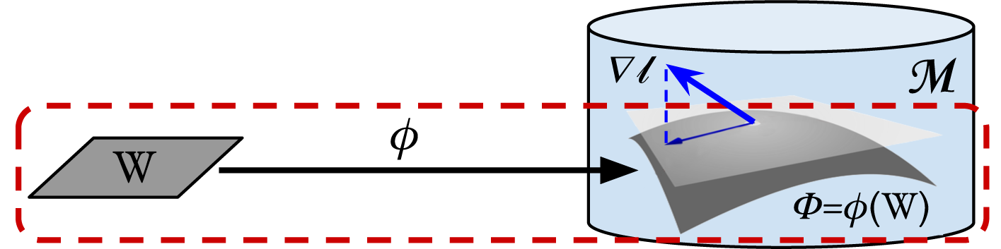
Figure 1: Most existing work on natural gradient focuses on the red dashed regime, where $\phi$ is a mapping from the parameter space $W$ to the parameterized functional space $\Phi=\phi(W)$. Natural gradient decreases the objective $\ell$ along the gradient flow line on $\Phi$ under a chosen Riemannian metric, instead of using the standard Euclidean metric on $W$. However, the functional gradient $\nabla\ell$ at any point of $\Phi$ need not lie in the tangent space to $\Phi$.

To the best of our knowledge, this is a more complete picture of natural gradient than has appeared in the machine learning literature, and is a novel assembling of known techniques from Sobolev spaces, RKHS, functional gradients, and Riemmannian geometry. We now summarize the contributions of this work, which also serves as an outline for the rest of the paper.

• In §2, we address the relationship between gradient flow on $\phi(W)$ and gradient flow on ${\mathcal{M}}$. The main theoretical result is Proposition 2.3, which shows that the inverse of metric matrix of natural gradient is in fact a consequence of the orthonormal projection from $\mathcal{M}$ onto $\Phi$.

• For standard empirical loss functions, we show in §3 that the gradient vector field on ${\mathcal{M}}$ with respect to the $L^{2}$ metric does not exist, as it is formally a sum of delta functions. Surprisingly, we also note that the formal/mechanical $L^{2}$ gradient projects to the correct $L^{2}$-induced gradient on $\phi(W).$

• In §4, Lemma 4.1 and Proposition 4.2, we prove that for $s>s_{0}$, the gradient flow on ${\mathcal{M}}$ in the $H_{s}$ metric is well-defined and projects to the $H_{s}$-induced gradient flow on $\phi(W)$, and hence pulls back to gradient flow on $W$ with respect to the natural metric. The main advantage of the $H_{s}$ metric is that delta functions are in the dual space $H_{s}^{*},$ which is not true for $L^{2}.$

• In §5, we discuss the differences between natural/pullback metrics and pushforward (Euclidean) metrics. In §5.1, we consider $H_{s}$ as an RKHS and characterize tangent spaces of $\Phi$ corresponding to different $w$ as a family of RKHS’s with corresponding projection kernels parameterized by $w$. In §5.2, we incorporate the standard (Enclidean) pushforward metric into this projection picture and relate it to the NTK kernel. A novel automatic orthonormality property of NTK-like/pushforward kernels is established in Proposition 5.1. As an example, in §5.3 we reformulate the notion of flatness in (Dinh et al., 2017) in terms of the pullback metric and show that it has the advantage of being coordinate-free, which was not enjoyed by its original definition using the pushforward metric.

• In §6 we discuss several critical computational techniques for implementing our Sobolev Natural Gradient. We first suggest an approximation of the Sobolev metric tensor by projecting it to the subspace spanned by evaluation functions at the training set. We then compute the Sobolev kernel as in (Wendland, 2004) and adapt the Kronecker-factored approximation to efficiently approximate the Sobolev Natural Gradient. Experimental results of our approach compared with Amari’s natural gradient baseline are included to demonstrate the potential of the Sobolev natural gradient.

Future work is discussed in §7. Proofs and Sobolev space technicalities are gathered in Appendices A and B. Appendix C contains experimental details and more results. Appendix D gives an example of the exact pullback metric computation in our framework for a simple neural network. Appendix E proves a stand-alone Riemannian version of primal and mirror descent on $W$ with the natural metric, under the assumption that the loss function on $\phi(W)$ pulls back to a convex function on $W$.

2 The Theoretical Setup

In supervised learning, we typically want to learn an optimal function $f:\mathbb{R}^{n}\to\mathbb{R}^{m}$, or more generally $f:M\to N$, where $M,N$ are $n$-dimensional, $m$-dimensional manifolds, respectively. Here an optimal function minimizes some cost function $F:{\mathcal{M}}\to\mathbb{R}$, where ${\mathcal{M}}$ is the space of candidate functions.

When function approximation is applied, $f$ is parameterized by some parameter vector of finite dimension, and the general situation can be described by the following simple diagram:

(1)

Here ${\mathcal{M}}={\mathcal{M}}(M,N)$ is a space of smooth maps from a manifold $M$ to a manifold $N$. ${\mathcal{M}}$ is an infinite dimensional manifold with a reasonable (high Sobolev or Fréchet) topology. The parameter space $W$, also a manifold, is usually a compact subset of a Euclidean space, and $\phi:W\to{\mathcal{M}}$ is the parametrization of the image $\phi(W)\subset{\mathcal{M}}$. $F$ is the loss function, and $\widetilde{F}=F\circ\phi$ makes the diagram commute.

We always assume that $\phi$ be an immersion, i.e., at every $w\in W$, the differential $d\phi_{w}:T_{w}W\to T_{\phi(w)}\phi(W)$ must be injective. Here $T_{w}W$ is the tangent space to $W$ at $w$, and similarly for $T_{\phi(w)}\phi(W)$. If this condition fails, then for a fixed metric $\bar{g}$ on ${\mathcal{M}}$, the pullback metric on $X,Y\in T_{w}W$

$$(\phi^{*}\bar{g})(X,Y):=\bar{g}(d\phi(X),d\phi(Y))$$ (2)

will be degenerate if $X\in{\rm ker}(d\phi).$ Here $\bar{g}$ is a Riemannian metric on ${\mathcal{M}}.$ In Appendix A.1, we discuss a work around for a particular case in the literature where $\phi$ is not an immersion.

2.1 Smooth gradients, orthogonal projection, and pullback metric

For a metric $\bar{g}$ on ${\mathcal{M}}$, we want to study the gradient flow of $F$ on the image $\Phi:=\phi(W)$, and this should be equivalent to studying gradient flow for $\widetilde{F}$ on $W$ via Amari’s natural gradient (Amari, 1998). Of course, to define the gradient, $F$ needs to be smooth (or at least Fréchet differentiable), which we assume here and treat more carefully in §3. Even this is not enough to assure that $\nabla F$ exists on ${\mathcal{M}}$, as discussed in §3. We also have to distinguish between the gradient flow lines of $F$ in ${\mathcal{M}}$ and the flow lines on $\Phi$. Indeed, a gradient flow line of $F$ starting in $\Phi$ will not stay in $\Phi$ in general, since $\nabla F$ need not point in $\Phi$ directions.

The following lemma establishes the relationship between gradient flow in ${\mathcal{M}}$ and flows on $\Phi$, and the equivalence between pullback gradients on the parameter space $W$ and gradients on $\Phi$ in the function space.

Lemma 2.1.

(i) The gradient flow on $\Phi=\phi(W)$ for $F|_{\Phi}$ is given by the flow of $P(\nabla F)$, where $P=P_{\phi(w)}$ is the orthogonal projection from $T_{\phi(w)}{\mathcal{M}}$ to $T_{\phi(w)}\Phi$.

(ii) Let ${\mathcal{M}}$ have a Riemannian metric $\bar{g}$, and let $\widetilde{g}=\phi^{*}\bar{g}$ be the pullback metric on $W$. Then $d\phi(\nabla_{\widetilde{g}}\widetilde{F})=\nabla_{\bar{g}}F$, and $\gamma(t)$ is a gradient flow line of $\widetilde{F}$ with respect to $\widetilde{g}$ iff $\phi(\gamma(t))$ is a gradient flow line of $F|_{\Phi}$.

Remark 2.2.

Lemma 2.1(ii) fails if we do not put the pullback metric $\widetilde{g}=\phi^{*}\bar{g}$ on $W$. In particular, for $W\subset\mathbb{R}^{n}$, the lemma fails if we use the Euclidean metric on $W.$

By this Lemma, we need to compute $P(\nabla F)$.

Proposition 2.3.

The orthogonal projection of $\nabla F$ onto $\phi(W)$ is

$$P(\nabla F)=\widetilde{g}^{ij}\left\langle\nabla F,\frac{\partial\phi}{\partial\theta^{i}}\right\rangle\frac{\partial\phi}{\partial\theta^{j}},$$ (3)

where $\widetilde{g}=\phi^{*}\bar{g}$ is the pullback metric on $W$.

Thus gradient flow lines for $\widetilde{F}$ are computed with respect to $\widetilde{g}$. From standard formulas in Riemannian geometry (Rosenberg, 1997, §1.2.3), the gradient of $\widetilde{F}$ is given by

$$\nabla\widetilde{F}=\widetilde{g}^{ij}\frac{\partial\widetilde{F}}{\partial\theta^{i}}\frac{\partial}{\partial\theta^{j}},$$ (4)

in local coordinates $\{\theta^{i}\}$ on $W$. Since $\phi:W\to\phi(W)$ is a diffeomorphism, (3) and (4) are equivalent. Again, if we used the Euclidean metric we would replace $\widetilde{g}^{ij}$ with $\delta^{ij}$, which certainly introduces error. Proofs for this section are in Appendix A.

3 $L^{2}$ Gradients of the Empirical Loss

In this section, we discuss the most commonly used setting of ${\mathcal{M}}$ in supervised machine learning, where the target space $N$ is $\mathbb{R}^{n}$, and the loss function $F$ is some empirical loss. In this case, ${\mathcal{M}}$ is an infinite dimensional vector space, so we have to specify its topology. For the easiest topology, the one induced by the $L^{2}$ inner product, we prove that the gradient of the loss function exists only formally/mechanically, although its projection to a finite dimensional parametrized submanifold $\Phi$ gives the correct formula for the gradient on $\Phi$. This lack of rigor motivates the use of Sobolev space topologies in §4.

A typical choice of empirical loss term on ${\mathcal{M}}$ is the mean squared loss

$$\ell_{E}(f)=\frac{1}{2}\sum_{i=1}^{k}d^{2}(f(x_{i}),y_{i}),$$ (5)

for a set $\{(x_{i},y_{i})\}^{k}_{i=1}\subset M\times\mathbb{R}^{n}$ of training data. Let $f:M\to\mathbb{R}^{n}$ have components $f^{j}:M\to\mathbb{R}$, and let $\delta_{i}$ be the “$\delta$-vector field”, $\delta_{i}(f^{j})=f^{j}(x_{i})\in\mathbb{R}$. We informally and incorrectly consider $\delta_{i}$ to be a function on $M$ with $\int_{M}\delta_{i}r=r(x_{i})$ for $r\in C^{\infty}(M)$. The integral is with respect to some volume form on $M$, so we are formally working with the $L^{2}$ inner product.

Take a curve $f_{t}\in{\mathcal{M}}$ with $f_{0}=f$, and set $h=\dot{f}_{t}|_{t=0}\in T_{f}{\mathcal{M}}\simeq{\mathcal{M}}.$ In this formal computation, we ignore the nontrivial question of the topologies on ${\mathcal{M}}$ and $T_{f}{\mathcal{M}}$. Then the differential $d\ell_{E}$ at $f$, denoted $d\ell_{E,f}:T_{f}{\mathcal{M}}\to\mathbb{R}$, satisfies

$$d\ell_{E,f}(h) =\frac{d}{dt}\biggl{|}_{{}_{t=0}}\frac{1}{2}\sum_{i}d^{2}(f_{t}(x_{i}),y_{i})=\frac{d}{dt}\biggl{|}_{{}_{t=0}}\frac{1}{2}\sum_{i}\sum_{j=1}^{n}(f_{t}^{j}(x_{i})-y_{i}^{j})^{2}$$ (6)

$$=\sum_{i}\sum_{j=1}^{n}(f^{j}(x_{i})-y_{i}^{j})h^{j}(x_{i}).$$

Thus we formally get $d\ell_{E,f}(h)=\int_{M}\sum_{j}\left(\sum_{i}(f^{j}(x_{i})-y_{i}^{j})\delta_{i}\right)h^{j}.$ We expect $d\ell_{E,f}(h)=$
$\langle\nabla\ell_{E,f},h\rangle_{L^{2}}=\int_{M}\sum_{j}(\nabla\ell_{E,f})^{j}\cdot h^{j},$ where $\cdot=\cdot_{E}$ is the Euclidean dot product. This equation is again formal, since a linear functional $\ell:{\mathcal{H}}\to\mathbb{R}$ on a Hilbert space ${\mathcal{H}}$ satisfies $\ell(h)=\langle w,h\rangle$ for some $w\in{\mathcal{H}}$ iff $\ell$ is continuous. Since we haven’t specified the topology on ${\mathcal{M}}$, we can’t discuss continuity of $d\ell_{E}.$ In any case, the formal gradient of $\ell_{E}$ at $f$ has $j^{\rm th}$ component given by

$$\left(\nabla\ell_{E,f}\right)^{j}=\sum_{i}(f(x_{i})-y_{i})^{j}\delta_{i}.$$ (7)

In other words, the gradient of the empirical loss (5) is formally a sum of delta functions. Since delta functions are not $L^{2}$ functions, the $L^{2}$ gradient does not exist.

We can also compute the formal gradient of $\ell_{E}$ restricted to $\Phi=\phi(W).$ By Proposition 2.3, we get

$$\nabla(\ell_{E}|_{\Phi})_{f} =\widetilde{g}^{kj}\left\langle\nabla\ell_{E,f},\frac{\partial\phi}{\partial\theta^{k}}\right\rangle\frac{\partial\phi}{\partial\theta^{j}}=\widetilde{g}^{kj}\left(\int_{M}\nabla\ell_{E,f}\cdot\frac{\partial\phi}{\partial\theta^{k}}\right)\frac{\partial\phi}{\partial\theta^{j}}$$ (8)

$$=\widetilde{g}^{kj}\left(\int_{M}\sum_{i}(f(x_{i})-y_{i})\delta_{i}\cdot\frac{\partial\phi}{\partial\theta^{k}}\right)\frac{\partial\phi}{\partial\theta^{j}}=\widetilde{g}^{kj}\sum_{i}\left((f(x_{i})-y_{i})\cdot_{E}\frac{\partial\phi}{\partial\theta^{k}}\biggl{|}_{{}_{x_{i}}}\right)\frac{\partial\phi}{\partial\theta^{j}}.$$

Of course, the gradient of $\ell_{E}|_{\Phi}$ exists on the finite dimensional manifold $\Phi$ and equals $d(\nabla_{\widetilde{g}}(\ell_{E}\circ\phi))$ by Lemma 2.1(ii). Thus at $f=\phi(\theta_{0}),$

$$\nabla(\ell_{E}|_{\Phi})_{f} =d\left(\widetilde{g}^{kj}\frac{\partial(\ell_{E}\circ\phi)}{\partial\theta^{k}}\frac{\partial}{\partial\theta^{j}}\right)=\widetilde{g}^{kj}\frac{\partial(\ell_{E}\circ\phi)}{\partial\theta^{k}}\frac{\partial\phi}{\partial\theta^{j}}$$ (9)

$$=\widetilde{g}^{kj}\sum_{i}\left((f(x_{i})-y_{i})\cdot_{E}\frac{\partial\phi}{\partial\theta^{k}}\biggl{|}_{{}_{x_{i}}}\right)\frac{\partial\phi}{\partial\theta^{j}}$$

Therefore the formal computation (8) on the infinite dimensional space ${\mathcal{M}}$ projects correctly to the finite dimensional space $\Phi.$ We find this surprising.

4 Sobolev Spaces and RKHS Theory

To addresss the concerns about the delta functions appearing in the gradient of the empirical loss, we rigorously compute the gradient of the empirical loss by introducing a Sobolev space topology/norm on ${\mathcal{M}}$. These norms make ${\mathcal{M}}$ an RKHS, and in the next section, we will make the relationship between general RKHS theory and Sobolev spaces more explicit.

To make the computations of $d\ell_{E,f}(h)$ in §3 rigorous, we have to pick a framework in which delta functions are well defined. We can either do this using the general theory of RKHSs, or we focus on a particular RKHS. We start with the particular choice of Sobolev space, as it generalizes to ${\mathcal{M}}(M,N)$, and discuss the general RKHS case in §5.1.

An overview of the Sobolev space is given in Appendix B. Following the notations therein, let ${\mathcal{M}}(M,\mathbb{R}^{n}):=H_{s}(M,\mathbb{R}^{n})$ now denote functions $f:M\to\mathbb{R}^{n}$ whose coordinate functions $f^{j}$ lie in the $s$-Sobolev space for some fixed integer $s>{\rm dim}(M)/2.$ In (6), $d\ell_{E,f}:T_{f}{\mathcal{M}}\simeq{\mathcal{M}}\to\mathbb{R}$ is a continuous linear functional on ${\mathcal{M}},$ because convergence in $H_{s}$ norm implies pointwise convergence by the Sobolev Embedding Theorem. Thus $d\ell_{E,f}(h)=\langle\nabla\ell_{E,f},h\rangle_{s}$ defines $\nabla\ell_{E,f}$ as an element of ${\mathcal{M}}.$ In contrast, $h\mapsto d\ell_{E,f}(h)$ is not a continuous linear functional on $L^{2}$, so the $L^{2}$ gradient does not exist.

Let $[\boldsymbol{\delta}_{x_{i}}(h)]^{j}=\delta_{x_{i}}h^{j}=h^{j}(x_{i})$ be the “$\delta$-vector” that evaluates each component of $h\in{\mathcal{M}}$ at the point $x_{i}.$ As above, there exists $d_{x_{i}}\in H_{s}(M)$ such that $\langle d_{x_{i}},h^{j}\rangle_{s}=\delta_{x_{i}}(h^{j})=h^{j}(x_{i})$ (see (33)). Let $\boldsymbol{d}_{x_{i}}$ be the diagonal matrix with diagonal entries $(d_{x_{i}},\ldots,d_{x_{i}})$.

The following results apply to more general empirical loss functions. Proofs are in Appendix A.3.

Lemma 4.1.

For $L=L(z,w):\mathbb{R}^{n}\times\mathbb{R}^{n}\to\mathbb{R}$ a differentiable function, the $H_{s}$-gradient of the $L$-empirical loss function $\ell_{L}(f)=\sum_{i}L(f(x_{i}),y_{i})$ on ${\mathcal{M}}=H_{s}(M,\mathbb{R}^{n})$ is given by

$$\nabla\ell_{L,f}=\sum_{i}\boldsymbol{d}_{x_{i}}(\nabla^{E}L_{z}(f(x_{i}),y_{i})).$$

Here $\nabla^{E}L_{z}$ is the Euclidean gradient of $L$ in the $z$ direction. The important question of computing $\boldsymbol{d}_{x_{i}}$ is treated in Appendix B. Although $\nabla\ell_{L,f}\in H_{s}(M,\mathbb{R}^{n})\subset L^{2}(M,\mathbb{R}^{n})$ for all $f$, we emphasize that $\nabla\ell_{L,f}$ is the $H_{s}$ and not the $L^{2}$ gradient, which doesn’t exist.

By Proposition 2.3, we can project $\nabla\ell_{L,f}$ to the tangent space of $\Phi=\phi(W)$ inside the Sobolev space $T_{f}{\mathcal{M}}\simeq H_{s}(M,\mathbb{R}^{n})$.

Proposition 4.2.

For $L=L(z,w):\mathbb{R}^{n}\times\mathbb{R}^{n}\to\mathbb{R}$ a differentiable function, the projection of the $H_{s}$-gradient of the $L$-empirical loss function $\ell_{L}(f)=\sum_{i}L(f(x_{i}),y_{i})$ to $\Phi=\phi(W)$ equals

$$P\nabla\ell_{L,f}=\widetilde{g}_{s}^{k\ell}\sum_{i}\left(\nabla^{E}L_{z}(f(x_{i}),y_{i})\cdot_{E}\frac{\partial\phi}{\partial\theta^{k}}\biggl{|}_{{}_{x_{i}}}\right)\frac{\partial\phi}{\partial\theta^{\ell}},$$ (10)

where $\widetilde{g}_{s}$ is the pullback to $W$ of the $s$-Sobolev inner product $\langle\cdot,\cdot\rangle_{s^{n}}$ on ${\mathcal{M}}=H_{s}(M,\mathbb{R}^{n})$.

We emphasize that the $\widetilde{g}^{k\ell}_{s}$ depend on the choice of $H_{s}$ norm. For $s$ an even integer, the $H_{s}$ inner product is equivalent to the inner product $\langle X,Y\rangle^{\prime}_{s}=\int_{\mathbb{R}^{n}}(1+\Delta)^{s/2}X\cdot_{\mathbb{R}^{m}}Y,$ where $\Delta$ is the Euclidean Laplacian acting componentwise on $X$, by the basic elliptic estimate (Gilkey, 1995, §1.3). This inner product is computable but exponentially expensive in $s.$ We call both (10) and its pullback to $W$ the Sobolev Natural Gradient, and discuss computational techniques to approximate it in §6.

5 Pushforward vs. Pullback Metrics

In this section, we compare pushforward metrics and pullback/natural metrics. In §5.1, we relate the Sobolev perspective of natural gradient presented in §4 with RKHS theory. In §5.2, we discuss NTK methods as a pushforward metric, showing that the pushforward metric fits into the RKHS framework of §5.1 and NTK-like kernels enjoy a nice automatic orthonormality property. In §5.3, we treat the flatness of a loss surface in both the pushforward and pullback context, as an example where the pullback metric has the strong advantage of giving a coordinate-free definition of flatness.

5.1 An RKHS perspective

As a Hilbert space of functions on which the evaluation/delta functions $\delta_{x}$ are continuous, ${\mathcal{H}}:=H_{s}$ is an RKHS. In the notation of §3, the reproducing or Mercer kernel is $K_{\mathcal{H}}^{ij}(x,y):=d_{x}(y)\delta^{i}_{j}.$ In the simplest case $M=\mathbb{R}^{n},$ we compute $d_{x}$ in Appendix B.

As in any RKHS, $\delta_{x_{i}}(f^{j})=\langle d_{x_{i}},f^{j}\rangle_{\mathcal{H}_{0}}$ for some $d_{x_{i}}\in\mathcal{H}_{0}$, where $\mathcal{H}_{0}$ is the scalar-value RKHS corresponding to each component of $f$. For vector-value RKHS $\mathcal{H}$, the reproducing property is

$$\langle K_{\mathcal{H}}(x,\cdot),f\rangle_{\mathcal{H}}=(\langle K_{\mathcal{H}}^{1}(x,\cdot),f\rangle,\ldots,\langle K_{\mathcal{H}}^{n}(x,\cdot),f\rangle)=(f^{1}(x),\ldots,f^{n}(x))=f(x).$$

The proof of Lemma 4.1 carries over to give

$$\nabla\ell_{L,f}=\sum_{i}K_{\mathcal{H}}(x_{i},\cdot)\nabla^{E}L_{z}(f(x_{i}),y_{i}).$$ (11)

For a particular choice of $K_{{\mathcal{H}}}$, this may be feasible to compute. In particular, this can be applied to stochastic gradient descent in our function space:

$$f_{t}=f_{t-1}-\eta_{t}\nabla\ell_{L,f_{t-1}},$$ (12)

where $\eta_{t}$ is the step size. If we apply (12) to a sequence of data points $(x_{1},y_{1}),(x_{2},y_{2}),\cdots,(x_{T},y_{T})$ with the initial condition $f_{0}(x)=0$, we get

$$f_{T}(x)=-\sum_{t=1}^{T}\eta_{t}K_{{\mathcal{H}}}(x_{t},x)\nabla L_{z}(z_{t},y_{t}).$$ (13)

Gradient descent in RKHS has been studied previously. See for example (Dieuleveut et al., 2016).

To further relate the RKHS perspective with the Sobolev perspective presented in §4, as we will see, projecting (11) to $\phi(W)$ precisely gives (10) of Proposition 4.2. We first emphasize that each $T_{f}\phi(W)$ becomes an RKHS for the $H_{s}$ metric using the $H_{s}$ orthogonal projection:

$$\boldsymbol{\delta_{x}}(g)=\langle g,P_{T_{f}\phi(W)}\boldsymbol{d}_{x}\rangle_{T_{f}\phi(W)}:=\langle g,\boldsymbol{d}_{x,f}\rangle_{T_{f}\phi(W)},\ {\rm for}\ g\in T_{f}\phi(W),$$

where $\boldsymbol{d}_{x,f}=P_{T_{f}\phi(W)}\boldsymbol{d}_{x}$, with corresponding positive definite kernel $K_{f}(x,x^{\prime})=\boldsymbol{d}_{x,f}(x^{\prime}).$ Thus it is more accurate to say that Sobolev theory produces a family of RKHSs parametrized by $w\in W$, with the corresponding reproducing kernel $K_{f}$, for $f=\phi(w)$, given by

$$K_{f}(x,x^{\prime}) =\boldsymbol{d}_{x,f}(x^{\prime})=(P_{T_{f}\phi(W)}\boldsymbol{d}_{x})(x^{\prime})=\sum_{i}\langle\boldsymbol{d}_{x},h_{i}\rangle_{\mathcal{H}}h_{i}(x^{\prime})=\sum_{i}h_{i}(x)\otimes h_{i}(x^{\prime}),$$ (14)

where $\{h_{i}\}$ is the orthonormal basis of $T_{f}\phi(W)$. Alternatively, by Proposition 2.3, we have

$$K_{f}(x,x^{\prime}) =(P_{T_{f}\phi(W)}\boldsymbol{d}_{x})(x^{\prime})=\tilde{g}^{ij}_{{\mathcal{H}}}\left\langle\boldsymbol{d}_{x},\frac{\partial\phi}{\partial\theta^{i}}\right\rangle_{\mathcal{H}}\frac{\partial\phi}{\partial\theta^{j}}(x^{\prime})=\tilde{g}^{ij}_{{\mathcal{H}}}\frac{\partial\phi}{\partial\theta^{i}}(x)\otimes\frac{\partial\phi}{\partial\theta^{j}}(x^{\prime}).$$ (15)

This yields an RKHS formulation of Proposition 4.2: by (11) and (15), for $P=P_{T_{f}\phi(W)},$

$$P\nabla\ell_{L,f} =\sum_{i}PK(x_{i},\cdot)\nabla^{E}L_{z}(f(x_{i}),y_{i})=\sum_{i}K_{f}(x_{i},\cdot)\nabla^{E}L_{z}(f(x_{i}),y_{i})$$ (16)

$$=\widetilde{g}_{s}^{k\ell}\sum_{i}\left(\nabla^{E}L_{z}(f(x_{i}),y_{i})\cdot_{E}\frac{\partial\phi}{\partial\theta^{k}}\biggl{|}_{{}_{x_{i}}}\right)\frac{\partial\phi}{\partial\theta^{\ell}},$$

which is (10).

While RKHS theory is general enough to apply to any finite basis, it does not specify which orthonormal basis, i.e., metric, is preferred. In §5.3, we argue with a concrete example that pullback metrics are better behaved than pushforward metrics.

5.2 NTK as a pushforward metric

In contrast to the kernel $K_{\mathcal{H}}^{ij}(x,y):=d_{x}(y)\delta^{i}_{j}$ in §5.1, in (Jacot et al., 2019, §4) the simpler NTK kernel is proposed:

$$\Theta^{(L)}(x,x^{\prime})=\sum_{i}\frac{\partial\phi}{\partial\theta^{i}}(x)\otimes\frac{\partial\phi}{\partial\theta^{i}}(x^{\prime}).$$ (17)

As in Proposition 2.3, where the gradient on $\phi(W)$ is obtained by a projection, this kernel follows from a surjection $S$ from $T_{f}{\mathcal{M}}$ to $T_{f}\phi(W)$ given by

$$S(v)(x^{\prime})=\left\langle\Theta^{(L)}(x,x^{\prime}),v(x)\right\rangle_{{\mathcal{H}}}=\sum_{i}\left\langle v,\frac{\partial\phi}{\partial\theta^{i}}\right\rangle_{\mathcal{H}}\frac{\partial\phi}{\partial\theta^{i}}(x^{\prime}).$$

While $S$ is similar to the orthonormal projection (10) in that $S|_{(T_{f}\phi(W))^{\perp}}=0$, $S$ is not a projection: $S^{2}$ and $S|_{T_{f}\phi(W)}$ are not the identity map. Thus flow lines for $\nabla\ell_{L,f}$ do not project to flow lines of $S\nabla\ell_{L,f}.$ Nevertheless, it is tempting to use the approximation

$$P\nabla\ell_{L,f}\approx S\nabla\ell_{L,f}=\sum_{i}\sum_{\ell}\left(\nabla^{E}L_{z}(f(x_{\ell}),y_{\ell})\cdot\frac{\partial\phi}{\partial\theta^{i}}\biggl{|}_{x_{\ell}}\right)\frac{\partial\phi}{\partial\theta^{i}}.$$ (18)

While (18) doesn’t involve the pullback metric $\tilde{g}^{ij}$ as in (10), (18) certainly introduces error. We could at least replace $X_{i}=\partial\phi/\partial\theta^{i}$ by their norm one versions $X_{i}/\|X_{i}\|_{s}.$ However, computing the $H_{s}$ norm of $X_{i}$ is not feasible.

While NTK methods have striking wide limits properties, to fit into the general framework of $\S\ref{sec:setup}$, we need metric on $T_{f}\phi(W)$ such that $S$ becomes an orthogonal projection. Forcing $S$ to be an orthogonal projection involves two steps: the first is making the $\{X_{i}\}$ an orthonormal basis of $T_{f}\phi(W)$, i.e.,

$$\left\langle\frac{\partial\phi}{\partial\theta^{i}},\frac{\partial\phi}{\partial\theta^{j}}\right\rangle=\delta_{ij},$$ (19)

which is addressed by the following Proposition 5.1. The second step is to define a normal space $\nu_{f}$ to $T_{f}\phi(W)$ inside $T_{f}{\mathcal{M}}$, so that any $v\in T_{f}\phi(W)$ can be decomposed into normal and tangential components, $v=v^{T}+v^{\nu}$, and we can define $S(v)=v^{T}.$ Since $T_{f}{\mathcal{M}}$ comes with a Riemannian metric $\bar{g}$ (e.g., the $H_{s}$ metrics), the easiest choice for a normal space is $\nu_{f}=\{w\in T_{f}{\mathcal{M}}:\langle w,w^{\prime}\rangle_{\bar{g}}=0,\ \forall w^{\prime}\in T_{f}\phi(W)\}.$ In summary, to make $S$ an orthogonal projection, we must alter $\bar{g}$ to a mixed metric which is given by (19) in directions tangent to $\phi(W)$ and by $\bar{g}$ in $\bar{g}$-normal directions.

This metric implicitly uses the pushforward $\phi_{*}g_{E}$ of the Euclidean metric from $W$ to $\phi(W)$: For a smooth map $\phi:W\to{\mathcal{M}}$ between manifolds, the pushforward of a metric $g$ on $W$ to a metric $\phi_{*}g$ on $\phi(W)$ is given by

$$(\phi_{*}g)(X,Y):=g((d\phi)^{-1}X,(d\phi)^{-1}Y),\ X,Y\in T\phi(W),$$

$\phi_{*}g$ exists iff $\phi$ is an immersion. We have $d\phi(\partial/\partial\theta^{i})=\partial\phi/\partial\theta^{i}$, so (19) is the pushforward $\phi_{*}g_{E}$ of the Euclidean metric on $W$.

While the construction of this mixed metric seems artificial, we now prove that (19) is automatically satisfied for the RKHS induced by the NTK kernel $\Theta^{(L)}$ on $\phi(W)$. This follows from the following Lemma for general finite dimensional functional spaces. As a result, $S$ is indeed an orthogonal projection under the mixed metric, and (23) becomes a special case of (15).

Proposition 5.1.

Given a finite dimensional functional space $\mathcal{F}\subset\{f:\mathcal{X}\to\mathbb{R}^{n}\}$ and any basis $\{b_{i}\}$ of $\mathcal{F}$, $\{b_{i}\}$ is an orthonormal basis of the RKHS corresponding to the kernel

$$K(x,x^{\prime})=\sum_{i}b_{i}(x)\otimes b_{i}(x^{\prime}).$$ (20)

The proof is in Appendix A.3. Note that this is a property of general finite dimensional function spaces regardless of whether or how they are parameterized. When $\mathcal{F}=T_{f}\phi(W)$ and $b_{i}=\frac{\partial\phi}{\partial\theta^{i}}$, we recover the NTK kernel (17) as a special case.

5.3 Pullback metric vs. pushforward metric: an example involving flatness

From a mathematical viewpoint, the pullback metric has better compatibility/naturality properties. For example, suppose $W\subset W^{\prime}$, and $\phi:W\to{\mathcal{M}}$ extends to $\phi^{\prime}:W^{\prime}\to{\mathcal{M}}$. Then the pullback metrics behave well: $(\phi^{\prime})^{*}\bar{g}=\phi^{*}\bar{g}$ for a metric $\bar{g}$ on ${\mathcal{M}}.$ In contrast, there is no relationship in general between $(\phi^{\prime})_{*}g_{E}$ and $\phi_{*}g_{E}$. In fact, there is no relationship between the pushforward metric and any metric on ${\mathcal{M}},$ so all insight coming from the geometry of ${\mathcal{M}}$ is lost. In contrast, the pullback metric retains all the information of $\bar{g}|_{\phi(W)}.$

This is not to say that the pushforward metric is never useful. The NTK approach works well when the trajectory stays near the initial condition $f_{0}=\phi(w_{0})$, as we are approximating the true trajectory in $\phi(W)$ by the linearized trajectory in $T_{f_{0}}\phi(W).$ This situation occurs in lazy training (Chizat et al., 2019).

A key point is that pullback metrics are independent of change of coordinates on the parameter space $W$, while pushforward metrics depend on a choice of coordinates. As a simple example, if we scale the standard coordinates $(x^{1},\ldots,x^{k})$ on $W\subset\mathbb{R}^{k}$ to $(y^{1},\ldots,y^{k})=(2x^{1},\ldots,2x^{k})$, then in (1) the pushforward metric $\phi_{*}g_{E}=\sum_{i}(\partial\phi/\partial x^{i})\otimes(\partial\phi/\partial x^{i})$ of the Euclidean metric on $W$ changes to $\sum_{i}(\partial\phi/\partial y^{i})\otimes(\partial\phi/\partial y^{i})=(1/4)\phi_{*}g_{E}.$ More generally, if $y=\alpha(x)$ is a change of coordinates on $W$ given by a diffeomorphism $\alpha,$ the pushforward metrics for the two coordinate systems will be very different. Thus the pushforward metric is useful only if we do not allow coordinate changes on $W$.

In contrast, the pullback metric is well behaved (“natural” in math terminology) with respect to coordinate changes. If $\bar{g}$ is a Riemannian metric on ${\mathcal{M}}$, then $(\phi\circ\alpha)^{*}\bar{g}=\alpha^{*}(\phi^{*}\bar{g}).$ In particular, for $v,w$ tangent vectors at a point in $W$, we have

$$\langle v,w\rangle_{(\phi\circ\alpha)^{*}\bar{g}}=\langle d\alpha(v),d\alpha(w)\rangle_{\phi^{*}\bar{g}}.$$ (21)

Since $v$ in the $x$-coordinate chart is identified with $d\alpha(v)$ in the $y=\alpha(x)$-coordinate chart, (21) says that the inner product of tangent vectors to $W$ is independent of chart for pullback metrics.

For the rest of this section, we give a concrete example in machine learning where these properties of the pullback metric have an explicit advantage over the pushforward metric. In particular, we consider the various notions of flatness associated to the basic setup (1) near a minimum. In (Dinh et al., 2017, §5), $\epsilon$-flatness of $\widetilde{F}:W\to\mathbb{R}$ near a minimum $w_{0}$ is defined by e.g., measuring the Euclidean volume of maximal sets $S\subset W$ on which $F(w)<F(w_{0})+\epsilon$ for all $w$ in $S$. The authors note that their definitions of flatness are not independent of scaling the Euclidean metric by different factors in different directions. Here the pushforward of the Euclidean metric is implicitly used. As above, scaling is the simplest version of a change of coordinates of the parameter space. Since this definition of flatness is not coordinate free, it has no intrinsic of differential geometric meaning.

This issue is discussed in (Dinh et al., 2017), Fig. 5. Under simple scaling of the $x$-axis, the graph of a function $f:\mathbb{R}\to\mathbb{R}$ will “look different.” Of course, $f$ is independent of scaling, but the graph looks different to an eye with an implicit fixed scale for the $x$-axis, i.e., from the point of view of a fixed coordinate chart.

We instead obtain the following coordinate free notion of flatness by measuring volumes in the pullback metric $\phi^{*}\bar{g}.$

Definition 5.2.

In the notation of (1), the $\epsilon$-flatness of $\widetilde{F}$ near a local minimum $w_{0}$ is $\int_{S}{\rm dvol}_{\phi^{*}\bar{g}}$ where $S$ is a maximal connected set such that ${\widetilde{F}}(S)\subset(\widetilde{F}(w_{0}),{\widetilde{F}}(w_{0})+\epsilon).$

Since $\int_{S}{\rm dvol}_{(\phi\circ\alpha)^{*}\bar{g}}=\int_{S}{\rm dvol}_{\phi^{*}\bar{g}}=\int_{\phi(S)}{\rm dvol}_{\bar{g}},$ for any orientation preserving diffeomorphism of $W$, $\epsilon$-flatness is independent of coordinates on $W$, and can be measured on $S$ or on ${\mathcal{M}}$. In contrast, the Euclidean volume of $S$ is not related to the volume of $\phi(S)\subset{\mathcal{M}}.$

6 Computational Techniques and Experimental Results

As shown in (16), in order to compute the Sobolev Natural Gradient on $W$, we have to efficiently compute the inverse of the Sobolev metric tensor $\widetilde{g}_{{\mathcal{H}},ij}$, which is analogous to the Fisher information matrix in Amari’s natural gradient. In §6.1, we discuss an RKHS-based approximation of $\widetilde{g}_{{\mathcal{H}},ij}$. In §6.2, we provide a practical computational method of $\widetilde{g}_{{\mathcal{H}},ij}$ based on the Kronecker-factored approximation (Martens and Grosse, 2015; Grosse and Martens, 2016). In §6.3, we report experimental results on supervised learning benchmarks.

6.1 An approximate computation of $\widetilde{g}_{{\mathcal{H}},ij}$

In general, it is not possible to exactly compute $\widetilde{g}_{{\mathcal{H}},ij}=\left\langle\frac{\partial\phi}{\partial\theta^{i}},\frac{\partial\phi}{\partial\theta^{j}}\right\rangle_{{\mathcal{H}}}$ for ${\mathcal{H}}=H_{s}$. We therefore resort to approximation. From (13), the functional gradient descent iterate $f_{T}$ lies in the subspace $K_{\mathcal{X}}$ of ${\mathcal{H}}$ spanned by $\{K_{{\mathcal{H}}}(x_{t},\cdot)\}^{T}_{t=1}$ for a given dataset $\mathcal{X}=\{x_{t}\}^{T}_{t=1}$. From the proof of Proposition 2.3 (in Appendix A), for any $f\in{\mathcal{H}}$, the projection is $P_{K_{\mathcal{X}}}f=K^{-1}_{ij}\left\langle f,K(x_{i},\cdot)\right\rangle_{{\mathcal{H}}}K(x_{j},\cdot)$, where $K_{ij}=\left\langle K(x_{i},\cdot),K(x_{j},\cdot)\right\rangle_{{\mathcal{H}}}$. We then approximate $\widetilde{g}_{{\mathcal{H}},ij}$ as follows,

$$\widetilde{g}_{{\mathcal{H}},ij} =\left\langle\frac{\partial\phi}{\partial\theta^{i}},\frac{\partial\phi}{\partial\theta^{j}}\right\rangle_{{\mathcal{H}}}\approx\left\langle P_{K_{{\mathcal{X}}}}\frac{\partial\phi}{\partial\theta^{i}},P_{K_{{\mathcal{X}}}}\frac{\partial\phi}{\partial\theta^{j}}\right\rangle_{{\mathcal{H}}}$$

$$=\left\langle K^{-1}_{ab}\left\langle\frac{\partial\phi}{\partial\theta^{i}},K(x_{a},\cdot)\right\rangle_{{\mathcal{H}}}K(x_{b},\cdot),K^{-1}_{cd}\left\langle\frac{\partial\phi}{\partial\theta^{j}},K(x_{c},\cdot)\right\rangle_{{\mathcal{H}}}K(x_{d},\cdot)\right\rangle_{{\mathcal{H}}}$$

$$=\left\langle\frac{\partial\phi}{\partial\theta^{i}},K(x_{a},\cdot)\right\rangle_{{\mathcal{H}}}K^{-1}_{ac}\left\langle\frac{\partial\phi}{\partial\theta^{j}},K(x_{c},\cdot)\right\rangle_{{\mathcal{H}}}$$

$$=\frac{\partial\phi}{\partial\theta^{i}}(x_{a})K^{-1}_{ac}\frac{\partial\phi}{\partial\theta^{j}}(x_{c}).$$ (22)

Note that by setting $K_{ij}$ to the identity matrix, (6.1) becomess the Gauss-Newton approximation of the natural gradient metric (Zhang et al., 2019c). For a practical implementation of (6.1) used in the next subsection, we only need to invert a $K_{ab}$ matrix of size $B\times B$, where $B$ is the mini-batch size of supervised training, which is quite manageable in practice.

Now all we need is to compute $K_{ij}=\left\langle K(x_{i},\cdot),K(x_{j},\cdot)\right\rangle_{{\mathcal{H}}}$ for all $x_{i},x_{j}\in{\mathcal{X}}.$ Since ${\mathcal{H}}$ is the Sobolev space $H_{s}$, the following Lemma computes $K_{ij}=d_{x_{i}}(x_{j})$.

Lemma 6.1.

For $s={\rm dim}(M)+3,$

$$d_{x_{i}}(x)=C_{n}e^{-\|x-x_{i}\|}(1+\|x-x_{i}\|),$$ (23)

where $C_{n}$ is some constant only depends on $n$.

This explicit formula for the Sobolev kernel is known in the literature, such as (Wendland, 2004, Theorem 6.13). We provide a full proof and its reduction to our specific form in Appendix B.

Even with (6.1), exact computation of the pullback metric for neural networks is in general extremely hard, we give such an example for a two-layer neural network in Appendix D. To efficiently approximate (6.1) in practice, in the next subsection, we adapt the Kronecker-factored approximation techniques (Martens and Grosse, 2015; Grosse and Martens, 2016).

6.2 Kronecker-factored approximation of $\widetilde{g}_{{\mathcal{H}}}$

Kronecker-factored Approximation Curvature (K-FAC) has been successfully used to approximate the Fisher information matrix for natural gradient/Newton methods. We now use fully-connected layers as an example to show how to adapt K-FAC (Martens and Grosse, 2015) to approximate $\widetilde{g}_{{\mathcal{H}}}$ in (6.1). Approximation techniques for convolutional layers can be similarly adapted from (Grosse and Martens, 2016). We omit standard K-FAC derivations and only focus on critical steps that are adapted for our approximation purposes. For full details of K-FAC, see (Martens and Grosse, 2015; Grosse and Martens, 2016).

As with the K-FAC approximation to the Fisher matrix, we first assume that entries of $\widetilde{g}_{{\mathcal{H}}}$ corresponding to different network layers are zero, which makes $\widetilde{g}_{{\mathcal{H}}}$ a block diagonal matrix, with each block corresponding to one layer of the network.

In the notation of (Martens and Grosse, 2015), the $\ell$-th fully-connected layer is defined by

$$\boldsymbol{s}_{\ell}=\bar{W}_{\ell}\bar{\boldsymbol{a}}_{\ell-1}\quad\bar{\boldsymbol{a}}_{\ell}=\psi_{\ell}(\boldsymbol{s}_{\ell}),$$

where $\bar{W}_{\ell}=(W_{\ell}\ \boldsymbol{b}_{\ell})$ denotes the matrix of layer bias and weights, $\bar{\boldsymbol{a}}_{\ell}=(\boldsymbol{a}^{T}_{\ell}\ 1)^{T}$ denotes the activations with an appended homogeneous dimension, and $\psi_{\ell}$ denotes the nonlinear activation function.

For $\widetilde{g}^{(\ell)}_{{\mathcal{H}}}$ the block of $\widetilde{g}_{{\mathcal{H}}}$ corresponding to the $\ell$-th layer, the argument of (Martens and Grosse, 2015) applied to (6.1) gives

$$\widetilde{g}^{(\ell)}_{{\mathcal{H}}}=\mathbb{E}_{K}\left[\bar{\boldsymbol{a}}_{\ell-1}\bar{\boldsymbol{a}}^{T}_{\ell-1}\otimes\mathcal{D}\boldsymbol{s}_{\ell}\mathcal{D}\boldsymbol{s}^{T}_{\ell}\right],$$ (24)

where $\mathcal{D}\boldsymbol{s}_{\ell}=\frac{\partial\phi}{\partial\boldsymbol{s}_{\ell}}$, $\otimes$ denotes the Kronecker product, and $\mathbb{E}_{K}$ is defined by

$$\mathbb{E}_{K}\left[X\otimes Y\right]=X(x_{i})K^{-1}_{ij}Y(x_{j}).$$

Just as K-FAC pushes the expectation of $\mathbb{E}\left[\bar{\boldsymbol{a}}_{\ell-1}\bar{\boldsymbol{a}}^{T}_{\ell-1}\otimes\mathcal{D}\boldsymbol{s}_{\ell}\mathcal{D}\boldsymbol{s}^{T}_{\ell}\right]$ inwards by assuming the independence of $\bar{\boldsymbol{a}}_{\ell-1}$ and $\boldsymbol{s}_{\ell}$, we apply the same trick to (24) by assuming the following $K^{-1}$-independence between $\bar{\boldsymbol{a}}_{\ell-1}$ and $\boldsymbol{s}_{\ell}$:

$$\mathbb{E}_{K}\left[\bar{\boldsymbol{a}}_{\ell-1}\bar{\boldsymbol{a}}^{T}_{\ell-1}\otimes\mathcal{D}\boldsymbol{s}_{\ell}\mathcal{D}\boldsymbol{s}^{T}_{\ell}\right]=\mathbb{E}_{K}\left[\bar{\boldsymbol{a}}_{\ell-1}\bar{\boldsymbol{a}}^{T}_{\ell-1}\right]\otimes\mathbb{E}_{K}\left[\mathcal{D}\boldsymbol{s}_{\ell}\mathcal{D}\boldsymbol{s}^{T}_{\ell}\right].$$ (25)

The rest of the computation follows the standard K-FAC for natural gradient. Let $\boldsymbol{A}_{\ell-1}$ and $\boldsymbol{S}_{\ell}$ be the Kronecker factors

$$\boldsymbol{A}_{\ell-1}=\mathbb{E}_{K}\left[\bar{\boldsymbol{a}}_{\ell-1}\bar{\boldsymbol{a}}^{T}_{\ell-1}\right]=\bar{\boldsymbol{a}}_{\ell-1}(x_{i})K^{-1}_{ij}\bar{\boldsymbol{a}}^{T}_{\ell-1}(x_{j}),$$

$$\boldsymbol{S}_{\ell}=\mathbb{E}_{K}\left[\mathcal{D}\boldsymbol{s}_{\ell}\mathcal{D}\boldsymbol{s}^{T}_{\ell}\right]=\mathcal{D}\boldsymbol{s}(x_{i})_{\ell}K^{-1}_{ij}\mathcal{D}\boldsymbol{s}^{T}_{\ell}(x_{j}).$$

Then our natural gradient for the $\ell$-th layer can be computed efficiently by solving the linear system,

$$\left(\widetilde{g}^{(\ell)}_{{\mathcal{H}}}\right)^{-1}\text{vec}(V_{\ell})=\left(\boldsymbol{A}_{\ell-1}\otimes\boldsymbol{S}_{\ell}\right)^{-1}\text{vec}(V_{\ell})=\left(\boldsymbol{A}_{\ell-1}^{-1}\otimes\boldsymbol{S}_{\ell}^{-1}\right)\text{vec}(V_{\ell})=\text{vec}(\boldsymbol{S}_{\ell}^{-1}V_{\ell}\boldsymbol{A}_{\ell-1}^{-1}),$$

where $\text{vec}(V_{\ell})$ denotes the vector form of the Euclidean gradients of loss with respect to the parameters of the $\ell$-th layer. All Kronecker factors $\boldsymbol{A}_{\ell}$ and $\boldsymbol{S}_{\ell}$ are estimated by moving averages over training batches.

6.3 Experimental results

Given that comparisons between natural gradient descent and Euclidean gradient descent have been conducted extensively in the literature (Zhang et al., 2019c, a) and that our proposed approach ends up being a new variant of natural gradient, our numerical experiments focus on comparing our Sobolev natural gradient (ours) with the most widely-used natural gradient (baseline) originally proposed by (Amari, 1998) in the supervised learning setting.

Since we borrow the K-FAC approximation techniques in designing an efficient computational method for our Sobolev natural gradient, we follow the settings of (Zhang et al., 2019c), which applies the K-FAC approximation to Amari’s natural gradient, to test both gradient methods on the VGG16 neural network on the CIFAR-10 and the CIFAR-100 supervised learning benchmarks. Our implementations and testbed are based on the PyTorch K-FAC codebase (Wang, 2019) provided by one of the co-authors of (Zhang et al., 2019c). For hyper-parameters of the baseline, we follow the grid searched results of (Wang, 2019). For our approach, we directly use most of the hyper-parameters optimized for the baseline, while tuning only the learning rate decay scheduling, and another scaling parameter which is only introduced by our method. We also confirm by experiments that switching to the set of hyper-parameters used by us does not bring any benefit to the performance of the baseline. Further details of the experimental setup and results are provided in Appendix C.

When comparing the natural gradient with the SGD, (Zhang et al., 2019c) trains natural gradients for 100 epochs while training the SGD for 200 epochs, highlighting the training efficiency of natural gradient methods. Following the same philosophy, in comparing the two natural gradient variants, we further shorten the training epochs to 50 in all our experiments, and we have found that the final performance is almost on par with that trained with 100 epochs. The training and testing behavior of ours vs. the baseline on CIFAR-10 and CIFAR-100 is shown in Figure 2 and Figure 3, respectively. While the final testing performance of both natural gradient variants are similar, as expected, our method shows a clear advantage regarding convergence speed, with the margin increased on the more challenging CIFAR-100 benchmark.

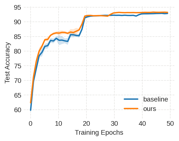
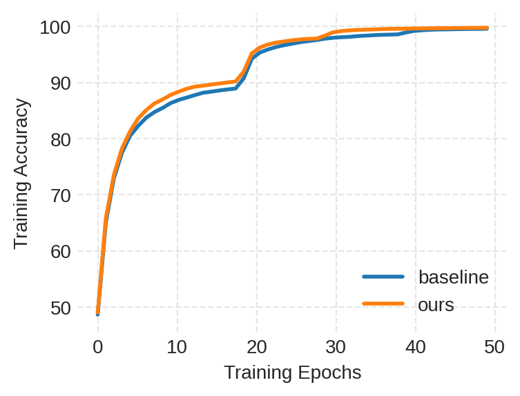
[Testing Accuracy] [Training Accuracy] [Training Loss]

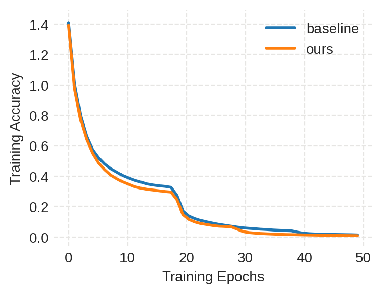
Figure 2: Training and testing behaviors of Sobolev Natural Gradient (ours) vs Amari’s Natural Gradient (baseline) on CIFAR-10. Results are averaged over four runs of different random seeds, with the shaded area corresponding to the standard deviation.

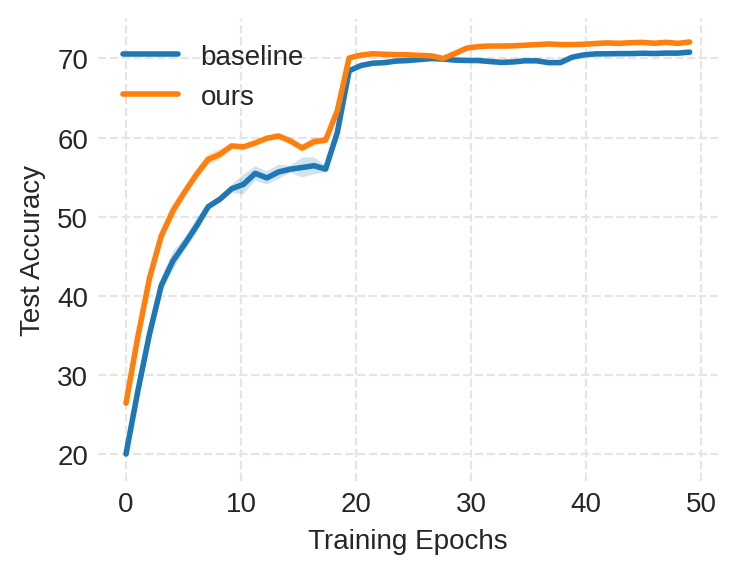
[Testing Accuracy] [Training Accuracy] [Training Loss]

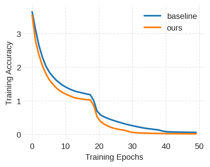
Figure 3: Training and testing behaviors of Sobolev Natural Gradient (ours) vs Amari’s Natural Gradient (baseline) on CIFAR-100. Results are averaged over four runs of different random seeds, with the shaded area corresponding to the standard deviation.

7 Future Work

We believe our work is just the beginning of fruitful results in both theory and practice of a broader view of natural gradient. From a theoretical viewpoint, it is worth studying what metrics in ${\mathcal{M}}$ lead to better convergence rate for natural gradient descent. It is even more interesting to investigate the relation between choices of metrics and the generalization ability, which we have not touched in current work. From a practical viewpoint, we hope to investigate better computational techniques for approximating $\widetilde{g}_{{\mathcal{H}}}$. In particular, we want to approximate it in the tangent spaces $T_{\phi(w)}{\mathcal{M}}$, which is in principle more accurate than approximating it on the subspace spanned by $\{K_{{\mathcal{H}}}(x_{t},\cdot)\}^{T}_{t=1}$ for the given training set, as done in §6.

Appendix A Technical details for §2, §4, and §5

A.1 A remark on immersions

There are examples of simple neural networks (Dinh et al., 2017, §3) where the immersion hypothesis fails. In particular, if for some $f\in{\rm Maps}(M,N)$ the level set $L_{f}=\phi^{-1}(f)$ is a positive dimensional submanifold of $W$, then $d\phi|_{L_{f}}=0.$ In this case, we assume that $W$ admits local slices $S$ for the level sets: $S$ is a union of submanifolds of $W$ such that there is one point in $S$ for each level set. If $S$ has just one component, it is called a global slice. In the example in (Dinh et al., 2017), the level sets in $W=\mathbb{R}^{+}\times\mathbb{R}^{+}$ are the hyperbolas $\{w_{1}w_{2}={\rm cons.}\}$, so a global slice is given e.g. by the lines $w_{1}={\rm cons.}$ or $w_{2}={\rm cons.}$ We then assume that $\phi|_{S}$ is an immersion. (In the example cited, the level sets are the orbits of a group action of $\mathbb{R}^{+}$ on $W$, namely $\lambda\cdot(w_{1},w_{2})=(\lambda w_{1},\lambda^{-1}w_{2}).$ For compact Lie group actions on manifolds, local slices always exist.)

A.2 Proofs for §2

Proof of Lemma 2.1.

(i) Take $X\in T_{\phi(w)}\Phi$ and a curve $\gamma(t)\subset\Phi$ with $\gamma(0)=\phi(w),\dot{\gamma}(0)=X.$ Then

$$d(F|_{\Phi})(X) =\frac{d}{dt}\biggl{|}_{{}_{t=0}}\left(F|_{\Phi}\right)(\gamma(t))=\frac{d}{dt}\biggl{|}_{{}_{t=0}}\left(F\right)(\gamma(t))$$

$$=\langle\nabla F,X\rangle_{\phi(w)}=\langle P(\nabla F),X\rangle_{\phi(w)}.$$

Since $d(F|_{\Phi})(X)=\langle\nabla(F|_{\Phi}),X\rangle$ determines $\nabla(F|_{\Phi}),$ we conclude that

$$P(\nabla F)=\nabla\left(F|_{\Phi}\right).$$ (26)

The result follows.

(ii) Take a gradient flow line $\gamma(t)$ for $\widetilde{F}$, so $\dot{\gamma}(t)=\nabla\widetilde{F}_{\gamma(t)}.$ Then $\phi\circ\gamma$ is a gradient flow line of $F|_{\Phi}$ iff

$$d\phi(\dot{\gamma})(\gamma(t))=(\phi\circ\gamma)\dot{}(t)=\nabla(F|_{\Phi})_{(\phi\circ\gamma)(t)}.$$

Substituting in $\dot{\gamma}(t)=\nabla\widetilde{F}_{\gamma(t)},$ and using (26), we need to show that

$$d\phi(\nabla\widetilde{F}_{w})=P(\nabla F_{\phi(w)}).$$ (27)

Take $\widetilde{X}\in T_{w}W$. Because $\phi$ is an isometry from $(W,\widetilde{g})$ to $(\Phi,\bar{g})$, we have for each $w$

$$\langle d\phi(\nabla\widetilde{F}),d\phi(\widetilde{X})\rangle_{\bar{g}} =\langle\nabla\widetilde{F},\widetilde{X}\rangle_{\widetilde{g}}=d\widetilde{F}(\widetilde{X})=d(F\circ\phi)(\widetilde{X})=dF\circ(d\phi(\widetilde{X}))$$

$$=\langle\nabla F,d\phi(\widetilde{X})\rangle_{\bar{g}}=\langle P(\nabla F),d\phi(\widetilde{X})\rangle_{\bar{g}}.$$

Since $d\phi(T_{w}W)$ spans $T_{\phi(w)}\Phi$, this proves (27) and $d\phi(\nabla\widetilde{F})=\nabla F$. $\Box$

Proof of Proposition 2.3. In general, we can compute the projection $P$ in a vector space as the solution to the minimization problem: the projection $P\boldsymbol{v}$ of a vector $\boldsymbol{v}$ onto a subspace $B$ is

$$P\boldsymbol{v}={\rm argmin}_{\boldsymbol{b}\in B}\|\boldsymbol{v}-\boldsymbol{b}\|^{2}.$$

If $\{b_{j}\}$ is a basis of $B$, we want ${\rm argmin}_{a^{i}\in\mathbb{R}}\|\boldsymbol{v}-\sum a_{i}\boldsymbol{b}_{i}\|^{2}.$ Taking first derivatives of $\|\boldsymbol{v}-\sum a_{i}\boldsymbol{b}_{i}\|^{2}$ with respect to $a^{i}$, we get

$$0=-2\langle v,b_{i}\rangle+2\sum_{j}a^{j}\langle b_{i},b_{j}\rangle.$$

For $\widetilde{g}=(\widetilde{g}_{ij})=(\langle b_{i},b_{j}\rangle)$, we get $a^{j}=\widetilde{g}^{ij}\langle\boldsymbol{v},b_{i}\rangle.$ Thus $P\boldsymbol{v}=\widetilde{g}^{ij}\langle\boldsymbol{v},b_{i}\rangle b_{j}.$ For $\boldsymbol{v}=\nabla F,b_{i}=\partial\phi/\partial\theta^{i}$, we recover (3). $\Box$

Proof of (4). For local coordinates $\{\theta^{i}\}$ on $W$, we have by definition

$$d\phi(\partial/\partial\theta^{i})=\partial\phi/\partial\theta^{i}.$$ (28)

By (27) we want to show

$$P(\nabla F)=\widetilde{g}^{ij}\frac{\partial\widetilde{F}}{\partial\theta^{i}}\frac{\partial\phi}{\partial\theta^{i}}.$$

Since

$$\frac{\partial\widetilde{F}}{\partial\theta^{i}}=d(F\circ\phi)(\partial/\partial\theta^{i})=dF(\partial\phi/\partial\theta^{i})=\left\langle\nabla F,\frac{\partial\phi}{\partial\theta^{i}}\right\rangle,$$

the proof follows from (3).

A.3 Proofs for §4 and §5

Proof of Lemma 4.1. We have

$$\langle\nabla\ell_{L,f},h\rangle_{s^{n}}=d\ell_{L,f}(h)=\frac{d}{dt}\biggl{|}_{{}_{t=0}}L(f_{t}(x_{i}),y_{i})=\sum_{i,j}\left(\frac{\partial L}{\partial z^{j}}(f(x_{i}),y_{i})\right)\cdot h^{j}(x_{i}).$$

For $\nabla^{E}L_{z}$ the Euclidean gradient of $L$ with respect to $z$ only, we have

$$\sum_{j}\left(\frac{\partial L}{\partial z^{j}}(f(x_{i}),y_{i})\right)\cdot h^{j}(x_{i}) =\sum_{j}(\nabla^{E}L_{z}(f(x),y_{i}))^{j}\cdot\langle d_{x_{i}},h^{j}\rangle_{s}=\langle\boldsymbol{d}_{x_{i}}(\nabla^{E}L_{z}(f(x),y_{i})),h\rangle_{s^{n}}.$$

$\Box$

Proof of Proposition 4.2.

$$P\nabla\ell_{L,f} =\widetilde{g}_{s}^{k\ell}\left\langle\sum_{i}\boldsymbol{d}_{x_{i}}(\nabla^{E}L_{z}(f(x_{i}),y_{i})),\frac{\partial\phi}{\partial\theta^{\ell}}\right\rangle_{s^{n}}\frac{\partial\phi}{\partial\theta^{j}}$$

$$=\widetilde{g}_{s}^{k\ell}\sum_{i,j}\left\langle[\boldsymbol{d}_{x_{i}}(\nabla^{E}L_{z}(f(x_{i}),y_{i}))]^{j},\frac{\partial\phi^{j}}{\partial\theta^{k}}\right\rangle_{s}\frac{\partial\phi}{\partial\theta^{\ell}}$$

$$=\widetilde{g}_{s}^{k\ell}\sum_{i}\left(\sum_{j}(\nabla^{E}L_{z}(f(x_{i}),y_{i}))^{j}\frac{\partial\phi^{j}}{\partial\theta^{k}}\biggl{|}_{{}_{x_{i}}}\right)\frac{\partial\phi}{\partial\theta^{\ell}}$$

$$=\widetilde{g}_{s}^{k\ell}\sum_{i}\left(\nabla^{E}L_{z}(f(x_{i}),y_{i})\cdot_{E}\frac{\partial\phi}{\partial\theta^{k}}\biggl{|}_{{}_{x_{i}}}\right)\frac{\partial\phi}{\partial\theta^{\ell}}.$$

$\Box$

We could also get this result by the approach in (9) for the $L^{2}$ ($s=0$) projection.

Proof of Proposition 5.1. Let $\mathcal{H}_{K}$ denote the RKHS corresponding to $K$. The $b_{i}$ are in the span of $\{K(x,\cdot),x\in\mathcal{X}\}$, so

$$b_{i}(\cdot) =\sum_{x\in\mathcal{X}}K(x,\cdot)C_{i}(x)=\sum_{x\in\mathcal{X}}C_{i}(x)^{T}\sum_{\ell}b_{\ell}(x)\otimes b_{\ell}(\cdot)$$ (29)

$$=\sum_{\ell}\left(\sum_{x\in\mathcal{X}}C_{i}(x)^{T}b_{\ell}(x)\right)b_{\ell}(\cdot)=\sum_{\ell}\alpha^{\ell}_{i}b_{\ell}(\cdot),$$

where $C_{i}:\mathcal{X}\to\mathbb{R}^{n}$ is some function. Since $\{b_{i}\}$ is a basis, the representation (29) is unique, i.e., $\alpha^{\ell}_{i}=\sum_{x\in\mathcal{X}}C_{i}(x)^{T}b_{\ell}(x)=\delta^{\ell}_{i}$. Thus by basic RKHS theory,

$$\langle b_{i},b_{j}\rangle_{K} =\left\langle\sum_{x\in\mathcal{X}}K(x,\cdot)C_{i}(x),\sum_{x^{\prime}\in\mathcal{X}}K(x^{\prime},\cdot)C_{j}(x^{\prime})\right\rangle_{K}=\sum_{x\in\mathcal{X}}\sum_{x^{\prime}\in\mathcal{X}}C_{i}(x)^{T}K(x,x^{\prime})C_{j}(x^{\prime})$$

$$=\sum_{x\in\mathcal{X}}\sum_{x^{\prime}\in\mathcal{X}}C_{i}(x)^{T}\sum_{\ell}b_{\ell}(x)\otimes b_{\ell}(x^{\prime})C_{j}(x^{\prime})$$

$$=\sum_{\ell}\left(\sum_{x\in\mathcal{X}}C_{i}(x)^{T}b_{\ell}(x)\right)\left(\sum_{x^{\prime}\in\mathcal{X}}C_{j}(x^{\prime})b_{\ell}(x^{\prime})\right)=\sum_{\ell}\alpha^{\ell}_{i}\alpha^{\ell}_{j}=\delta^{i}_{j},$$

where $\delta^{i}_{j}$ is the indicating function that equals $1$ when $i=j$ and $0$ otherwise. $\Box$

Appendix B Review of Sobolev spaces and the computation of $d_{x}$

B.1 Review of Sobolev spaces

We recall some basics of Sobolev space theory on manifolds $M$; for calculations in this paper, $M=\mathbb{R}^{n}$ with the Euclidean metric. Details for this material are in (Gilkey, 1995, Ch. 1).

Let $M$ be a closed manifold. For $f\in C^{\infty}(M)=C^{\infty}(M,\mathbb{C})$ and $s\gg 0$ a fixed integer, we usually let $H_{s}=H_{s}(M)$ be the Sobolev space given by the completion of $C^{\infty}(M)$ with respect to the norm

$$\|f\|_{s}^{2}=\sum_{|\alpha|\leq s}\|\partial^{\alpha}f\|_{2}^{2},$$

where $\|\cdot\|_{2}$ is the $L^{2}$ norm with respect to a fixed Riemannian metric on $M$. Here $\alpha=(\alpha^{1},\ldots,\alpha^{n})$ is a multi-index with $|\alpha|=\sum_{i}\alpha_{i}$, and $\partial^{\alpha}=\partial^{|\alpha|}/\partial x^{\alpha^{1}}\ldots\partial x^{\alpha^{n}}.$ Similarly, for $f=(f^{1},\ldots,f^{n})\in C^{\infty}(M,\mathbb{R}^{n}),$ we set $\|f\|_{s}^{2}=\sum_{j}\|f^{j}\|_{s}^{2}$. However, it is more efficient to use the equivalent norm

$$\|f\|_{s}^{2}=\int_{M}|\hat{f}(\xi)|^{2}(1+|\xi|^{2})^{s/2}\ d\xi^{1}\wedge\ldots\wedge d\xi^{n},$$

where we compute the Fourier transform and integral in local coordinates and use a partition of unity. In particular, the integral depends on choices of coordinates and the partition of unity. With this norm, $H_{s}(M)$ is a Hilbert space with respect to the inner product

$$\langle f,g\rangle_{s}=\int_{M}\hat{f}(\xi)\overline{\hat{g}(\xi)}(1+|\xi|^{2})^{s/2}\ d\xi.$$ (30)

Similarly, $H_{s}(M,\mathbb{R}^{n})$ has the inner product

$$\langle f,g\rangle_{s}=\int_{M}\sum_{j}\hat{f}_{j}(\xi)\overline{\hat{g}_{j}(\xi)}(1+|\xi|^{2})^{s/2}\ d\xi.$$

The advantage of (30) is that we can now define $H^{s}$ for any $s\in\mathbb{R}$, and we have the basic fact that there is a continuous nondegenerate pairing $H_{s}\otimes H_{-s}\to\mathbb{C}$, $f\otimes g\mapsto\int_{M}f\cdot\overline{g}\ {\rm dvol}.$ This implies

$$H_{s}^{*}\stackrel{{\scriptstyle\simeq}}{{\longrightarrow}}H_{-s}\ {\rm via}\ f\mapsto\left(g\mapsto\int_{M}f\cdot\overline{g}\ {\rm dvol}\right).$$ (31)

By the Sobolev Embedding Theorem, for $s>(n/2)+s^{\prime},$ $H_{s}(M)$ is continuously embedded in $C^{s^{\prime}}(M)$, the space of $s^{\prime}$ times continuously differentiable functions on $M$ with the sup norm. We always assume $s$ satisfies this lower bound for $s^{\prime}=0$. As a result, for any $x\in M$, the delta function $\delta_{x}$ is in $H_{s}^{*}(M)$: if $f_{i}\to f$ in $H_{s}$, then $f_{i}\to f$ in sup norm, so $\delta_{x}(f_{i})=f_{i}(x)\to f(x)=\delta_{x}(f).$ Thus there exists $d_{x}\in H_{s}(M)$ such that

$$\delta_{x}(f)=\langle d_{x},f\rangle_{s},\forall f\in H_{s}.$$

For $f\in H_{s}(M,\mathbb{R}^{m})$, we can extend the inner product by

$$\langle f,g\rangle_{s^{n}}=\sum_{j}\langle f^{j},g^{j}\rangle_{s},$$ (32)

and we can generalize the delta function to $\boldsymbol{\delta}_{x},$ where

$$\boldsymbol{\delta}_{x}(f)=f(x),\ i.e.,\ [\boldsymbol{\delta}_{x}(f)]^{j}=\langle d_{x},f^{j}\rangle_{s}.$$ (33)

B.2 Computation of $d_{x_{i}}$

Let $N(x_{i},\sigma)(x)$ be the multivariate normal distribution with mean $x_{i}$ and variance $\sigma=\sigma\cdot{\rm Id}.$ For $\sigma\approx 0$, $N(x_{i},\sigma)$ acts like a delta function: for $f\in H_{s}(\mathbb{R}^{n}),s>(n/2)+1,$

$$\lim_{\sigma\to 0}\int_{\mathbb{R}^{n}}N(x_{i},\sigma)(x)f(x)dx=f(x_{i}).$$

This uses that $f$ is continuous, so the delta function is a continuous functional on $H_{s}$, hence in $H_{-s}$, and $\lim_{\sigma\to 0}N(x_{i},\sigma)=\delta_{x_{i}}$ in $H_{-s}(\mathbb{R}^{n}).$ Therefore

$$\lim_{\sigma\to 0}\int_{\mathbb{R}^{n}}N(x_{i},\sigma)f(x)dx =f(x_{i})=\langle d_{x_{i}},f\rangle_{s}=\int_{\mathbb{R}^{n}}\widehat{d_{x_{i}}}(\xi)\hat{f}(\xi)(1+|\xi|^{2})^{s/2}d\xi$$

$$=\int_{\mathbb{R}}f(x)\mathcal{F}^{-1}\left(\widehat{d_{x_{i}}}(1+|\xi|^{2})^{s/2}\right),$$

with $\mathcal{F}^{-1}$ the inverse Fourier transform. (This uses the fact that the Fourier transform is a bijection on $H_{-s}$.) Thus $\delta_{x_{i}}=\mathcal{F}^{-1}\left(\widehat{d_{x_{i}}}(1+|\xi|^{2})^{s/2}\right)\in H_{-s}(\mathbb{R}^{n}).$ This implies $\widehat{d_{x_{i}}}=\mathcal{F}(\delta_{x_{i}})(1+|\xi|^{2})^{-s/2}$. Using $\mathcal{F}^{-1}(\mathcal{F}(f)g)=f*\mathcal{F}^{-1}(g)$, where $*$ is convolution, we get

$$d_{x_{i}}(x)$$

$$=\left(\delta_{x_{i}}*\mathcal{F}^{-1}\left((1+|\xi|^{2})^{-s/2}\right)\right)(x)=\lim_{\sigma\to 0}\int_{\mathbb{R}^{n}}N(x_{i},\sigma)(y)\mathcal{F}^{-1}\left((1+|\xi|^{2})^{-s/2}\right)(x-y)dy$$

$$=\mathcal{F}^{-1}\left((1+|\xi|^{2})^{-s/2}\right)(x-x_{i})=\frac{1}{(2\pi)^{n}}\int_{\mathbb{R}^{n}}e^{i(x-x_{i})\cdot\xi}(1+|\xi|^{2})^{-s/2}d\xi$$

$$=\frac{1}{(2\pi)}\int_{\mathbb{R}^{n}}\cos((x-x_{i})\cdot\xi)(1+|\xi|^{2})^{-s/2}d\xi,$$

since $\sin$ is an odd function.

We begin with the case $n=1$, so we are considering $H_{1}(\mathbb{R},\mathbb{R}).$ Set $A=s/2.$ We assume $s\in 2\mathbb{Z}$ for now. (Below, in Case II, we will have $s\in 2\mathbb{Z}+1$, but then we set $A=(s-n+1)/2$, so again $A\in\mathbb{Z}.$ Thus we can apply Lemma B.1.)

Lemma B.1.

$$d_{x_{i}}(x)=\frac{1}{2\pi}\int_{-\infty}^{\infty}e^{i|x-x_{i}|\xi}(1+\xi^{2})^{-A}d\xi=\frac{e^{-|x-x_{i}|}|x-x_{i}|^{A-1}}{2^{A}(A-1)!}\sum_{k=0}^{A-1}\frac{(A+k-1)!}{k!(A-k-1)!}(2|x-x_{i}|)^{-k}.$$

In particular,

$$d_{x_{i}}(x_{i})=\binom{2A-2}{A-1}2^{-2A+1}.$$

Proof B.2.

Fix $a\in\mathbb{R}$. We compute

$$\lim_{R\to\infty}\oint_{C_{R}}e^{iaz}(1+z^{2})^{-s/2},$$

where $C_{R}$ is the contour from $-R$ to $R$ and then the semicircle in the upper half plane centered at the origin and radius $R$, traveled counterclockwise. By the Jordan Lemma, the integral over the semicircle goes to zero as $R\to\infty$, so

$$\lim_{R\to\infty}\oint_{C_{R}}e^{iaz}(1+z^{2})^{-A}=\int_{-\infty}^{\infty}e^{iax}(1+x^{2})^{-A}dx,$$

the integral we want.

The only pole of the integrand inside the contour is at $z=i$, where $(1+z^{2})^{-A}=(i+z)^{-A}(-i+z)^{-A}$ contributes a pole of order $A.$ By the Cauchy residue formula and the standard formula for computing residues,

$$\oint_{C_{R}}e^{iaz}(1+z^{2})^{-A}$$

$$=2\pi i\ {\rm Res}_{z=i}e^{iaz}(1+z^{2})^{-A}$$

$$=2\pi i\frac{1}{(A-1)!}\frac{d^{A-1}}{dz^{A-1}}\biggl{|}_{z=i}(z-i)^{A}(1+z^{2})^{-A}e^{iaz}$$

$$=2\pi i\frac{1}{(A-1)!}\frac{d^{A-1}}{dz^{A-1}}\biggl{|}_{z=i}(z+i)^{-A}e^{iaz}$$

$$=2\pi i\frac{1}{(A-1)!}\sum_{k=0}^{A-1}\binom{A-1}{k}(-1)^{k}A(A+1)(A+k-1)(2i)^{-A-k}e^{-a}(ia)^{A-1-k}$$

$$=2\pi ie^{-a}\frac{1}{(A-1)!}\sum_{k=0}^{A-1}(-1)^{k}\frac{(A-1)!}{k!(A-k-1)!}\frac{(A+k-1)!}{(A-1)!}i^{-1-2k}2^{-A-k}a^{A-1-k}$$

$$=\frac{2\pi e^{-a}}{(A-1)!}\sum_{k=0}^{A-1}\frac{(A+k-1)!}{k!(A-k-1)!}2^{-A-k}a^{A-1-k}$$

$$=\frac{\pi e^{-a}a^{A-1}}{2^{A-1}(A-1)!}\sum_{k=0}^{A-1}\frac{(A+k-1)!}{k!(A-k-1)!}2^{-k}a^{-k}.$$

Letting $R\to\infty$, replacing $a$ by $|x-x_{i}|$, and remembering to divide by $2\pi$ in the definition of the Fourier transform, we get

$$d_{x_{i}}(x)=\frac{e^{-|x-x_{i}|}|x-x_{i}|^{A-1}}{2^{A}(A-1)!}\sum_{k=0}^{A-1}\frac{(A+k-1)!}{k!(A-k-1)!}(2|x-x_{i}|)^{-k}.$$

Note that for $x=x_{i}$, we get a nonzero contribution only for $k=A-1$, so the right hand side equals

$$\binom{2A-2}{A-1}2^{-2A+1}.$$

Remark B.3.

The modified Bessel function of the second kind satisfies

$$K_{\nu}(z)=\frac{\Gamma(\nu+1/2)(2z)^{\nu}}{\sqrt{\pi}}\int_{0}^{\infty}\cos(at)a^{-2\nu}\left(t^{2}+\left(\frac{z}{a}\right)^{2}\right)^{-\nu-1/2}dt,$$

for $a>0$ and $Re(\nu+1/2)>0.$ Combining this formula with the half-integer formula

$$K_{(A-1)+1/2}(\nu)=\sqrt{\pi/2\nu}\cdot e^{-\nu}\sum_{k=0}^{A-1}\frac{(A-1+k)!}{k!(A-1-k)!(2\nu)^{k}}$$

(Watson, 1922, p. 80, Eq. (12) and p. 172, Eq. (1)) gives another proof of Lemma B.1.

Now we consider the case of $H_{s}(\mathbb{R}^{n},\mathbb{R})$. Here

$$d_{x_{i}}(x)=\frac{1}{(2\pi)^{n}}\int_{\mathbb{R}^{n}}e^{i(x-x_{i})\cdot\xi}\left(1+|\xi|^{2}\right)^{-s/2}d\xi.$$ (34)

Assume $x_{i}\neq x.$ Find $B\in SO(n)$ with $Be_{n}=\frac{x-x_{i}}{|x-x_{i}|}.$ Then

$$\int_{\mathbb{R}^{n}}e^{i(x-x_{i})\cdot\xi}\left(1+|\xi|^{2}\right)^{-s/2}d\xi$$

$$=\int_{\mathbb{R}^{n}}e^{i(x-x_{i})\cdot B(\xi)}\left(1+|B(\xi)|^{2}\right)^{-s/2}\det(B)d\xi=\int_{\mathbb{R}^{n}}e^{i(B^{-1}(x-x_{i}))\cdot\xi}\left(1+|\xi|^{2}\right)^{-s/2}d\xi$$

$$=\int_{\mathbb{R}^{n}}e^{i|x-x_{i}|\xi_{n}}\left(1+|\xi|^{2}\right)^{-s/2}d\xi$$

$$=\int_{\mathbb{R}}e^{i|x-x_{i}|\xi_{n}}\left(\int_{\mathbb{R}^{n-1}}\left(1+\xi_{n}^{2}+\xi_{1}^{2}+\ldots+\xi_{n-1}^{2}\right)^{-s/2}d\xi_{1}\ldots d\xi_{n-1}\right)d\xi_{n}$$ (35)

$$=\int_{\mathbb{R}}e^{i|x-x_{i}|\xi_{n}}\left(\int_{\mathbb{R}^{n-1}}\left(1+\xi_{n}^{2}\right)^{-s/2}\left(1+\frac{\xi_{1}^{2}}{1+\xi_{n}^{2}}+\ldots+\frac{\xi_{n-1}^{2}}{1+\xi_{n}^{2}}\right)^{-s/2}d\xi_{1}\ldots d\xi_{n-1}\right)d\xi_{n}$$

$$\stackrel{{\scriptstyle\xi_{i}\mapsto\xi_{i}(1+\xi_{n}^{2})^{-1/2}}}{{=}}\int_{\mathbb{R}}e^{i|x-x_{i}|\xi_{n}}\left(1+\xi_{n}^{2}\right)^{-s/2+(n-1)/2}\left(\int_{\mathbb{R}^{n-1}}\left(1+\xi_{1}^{2}+\ldots+\xi_{n-1}^{2}\right)^{-s/2}d\xi_{1}\ldots d\xi_{n-1}\right)d\xi_{n}$$

$$=\left(\int_{\mathbb{R}}e^{i|x-x_{i}|\xi_{n}}\left(1+\xi_{n}^{2}\right)^{-s/2+(n-1)/2}d\xi_{n}\right)\left(\int_{0}^{\infty}\int_{S^{n-2}}(1+r^{2})^{-s/2}r^{n-2}drd\theta_{1}\ldots d\theta_{n-2}\right)$$

$$=\left(\int_{\mathbb{R}}e^{i|x-x_{i}|\xi_{n}}\left(1+\xi_{n}^{2}\right)^{-s/2+(n-1)/2}d\xi_{n}\right)\left(\int_{0}^{\infty}(1+r^{2})^{-s/2}r^{n-2}dr\right){\rm vol}(S^{n-2})$$

$$=\left(\int_{\mathbb{R}}e^{i|x-x_{i}|\xi_{n}}\left(1+\xi_{n}^{2}\right)^{-s/2+(n-1)/2}d\xi_{n}\right)\left(\int_{0}^{\infty}(1+r^{2})^{-s/2}r^{n-2}dr\right)\frac{2\pi^{\frac{n-1}{2}}}{\Gamma\left(\frac{n-1}{2}\right)}.$$

The first term on the last line is computed in Lemma B.1, and is valid for $-s/2+(n-1)/2<-1,$ i.e. for

$$s>n+1.$$

So we have to calculate $\int_{0}^{\infty}(1+r^{2})^{-s/2}r^{n-2}dr$.

Case I: $n$ odd, and we assume $s\in 2\mathbb{Z}.$

We use integration by parts repeatedly (and assume $s>n+3$):

$$\int_{0}^{\infty}(1+r^{2})^{-s/2}r^{n-2}dr$$

$$=\int_{0}^{\infty}\left[(1+r^{2})^{-s/2}\cdot\frac{2r}{-s/2+1}\right]r^{n-3}dr\left(\frac{-s/2+1}{2}\right)$$

$$=-\int_{0}^{\infty}(1+r^{2})^{-s/2+1}r^{n-4}dr\cdot\left(\frac{-s/2+1}{2}\right)(n-3)\ \ \ \ \ \ \ \ \ \ \ \ \ \ \ \ \ \ \ \ \ \ \ \ \ \ \ \ \ \text{(Step 1)}$$

$$=-\int_{0}^{\infty}\left[(1+r^{2})^{-s/2+1}\cdot\frac{2r}{-s/2+2}\right]r^{n-5}dr\cdot\frac{(-s/2+2)(-s/2+1)}{2^{2}}\cdot(n-3)$$

$$=\int_{0}^{\infty}(1+r^{2})^{-s/2+2}r^{n-6}dr\cdot\frac{(-s/2+2)(-s/2+1)}{2^{2}}\cdot(n-3)(n-5)\ \ \ \ \ \ \ \ \ \text{(Step 2)}.$$

To get the term $r^{1}$ in the integrand, we need $\frac{n-3}{2}$ steps. (The exponent drops by $2b+2$ at the $b^{\rm th}$ step, so solve $2b+2=n-1$ for $b$.) At Step $\frac{n-3}{2}$, the sign in front of the integral is $(-1)^{(n-3)/2}$, the exponent of $1+r^{2}$ is $-s/2+\frac{n-3}{2}=\frac{-s+n-3}{2}$, and the constant after the integral is

$$\frac{\left(-s/2+\frac{n-3}{2}\right)\left(-s/2+\frac{n-5}{2}\right)\cdot\ldots\cdot(-s/2+1)(n-3)(n-5)\cdot\ldots\cdot 2}{2^{\frac{n-3}{2}}}.$$

(For the final $2$ in the numerator, at the $b^{\rm th}$ step we get $n-(2b+1)=n-(n-3+1)=2.$) This equals

$$\frac{\left(-s+n-3\right)\left(-s+n-5\right)\cdot\ldots\cdot(-s+4)(-s+2)(n-3)!!}{2^{n-3}}$$

$$=(-1)^{\frac{n-3}{2}}\frac{(s-n+3)(s-n+5)\cdot\ldots\cdot(s-4)(s-2)(n-3)!!}{2^{n-3}}$$

$$=(-1)^{\frac{n-3}{2}}\frac{(s-2)!!(n-3)!!}{2^{n-3}(s-n+1)!!}.$$

Thus

$$\int_{0}^{\infty}(1+r^{2})^{-s/2}r^{n-2}dr$$

$$=(-1)^{\frac{n-3}{2}}\int_{0}^{\infty}(1+r^{2})^{(-s+n-3)/2}rdr\cdot(-1)^{\frac{n-3}{2}}\frac{(s-2)!!(n-3)!!}{2^{n-3}(s-n+1)!!}$$

$$=\frac{1}{s-n+1}\cdot\frac{(s-2)!!(n-3)!!}{2^{n-3}(s-n+1)!!}.$$

Note that this expression is valid for $s>n.$ Thus for $A=\frac{s-n+1}{2}$, with $s\in 2\mathbb{Z}+1,s\geq n+3$ (e.g., for $s=n+3,$ we have the requirements $A\in\mathbb{Z}$ and $s>n+1$),

$$d_{x_{i}}(x)$$ (36)

$$=\frac{1}{(2\pi)^{n}}\left(\int_{\mathbb{R}}e^{i|x-x_{i}|\xi}\left(1+\xi^{2}\right)^{-s/2+(n-1)/2}d\xi_{n}\right)\left(\int_{0}^{\infty}(1+r^{2})^{-s/2}r^{n-2}dr\right){\rm vol}(S^{n-2})$$

$$=\frac{1}{(2\pi)^{n}}\left(\int_{\mathbb{R}}e^{i|x-x_{i}|\xi}\left(1+\xi^{2}\right)^{-s/2+(n-1)/2}d\xi_{n}\right)\cdot\frac{1}{s-n+1}\cdot\frac{(s-2)!!(n-3)!!}{2^{n-3}(s-n+1)!!}\cdot\frac{2\pi^{\frac{n-1}{2}}}{\Gamma\left(\frac{n-1}{2}\right)}$$

$$=\frac{1}{\pi^{\frac{n+1}{2}}}\left(\int_{\mathbb{R}}e^{i|x-x_{i}|\xi}\left(1+\xi^{2}\right)^{-s/2+(n-1)/2}d\xi\right)\cdot\frac{1}{s-n+1}\cdot\frac{(s-2)!!(n-3)!!}{2^{2n-4}(s-n+1)!!}\cdot\frac{1}{\left(\frac{n-3}{2}\right)!}$$

$$=\frac{1}{\pi^{\frac{n+1}{2}}}\frac{e^{-|x-x_{i}|}|x-x_{i}|^{A-1}}{2^{A}(A-1)!}\sum_{k=0}^{A-1}\frac{(A+k-1)!}{k!(A-k-1)!}(2|x-x_{i}|)^{-k}$$

$$\qquad\cdot\frac{1}{s-n+1}\cdot\frac{(s-2)!!(n-3)!!}{2^{2n-4}(s-n+1)!!}\cdot\frac{1}{\left(\frac{n-3}{2}\right)!}.$$

To treat $x=x_{i}$, we can use the fact that $d_{x_{i}}(x)$ is highly differentiable, and let $x\to x_{i}$ in the last formula. As in the one-dimensional case, we get

$$d_{x_{i}}(x_{i})=\frac{1}{\pi^{\frac{n+1}{2}}}\binom{s-n-1}{\frac{s-n-1}{2}}2^{-s+n}\frac{1}{s-n+1}\cdot\frac{(s-2)!!(n-3)!!}{2^{2n-4}(s-n+1)!!}\cdot\frac{1}{\left(\frac{n-3}{2}\right)!}.$$

Case II: $n$ even and we assume $s\in 2\mathbb{Z}+1$.

Now it takes $\frac{n}{2}-1$ steps to reduce $\int_{0}^{\infty}(1+r^{2})^{-s/2}r^{n-2}dr$ to a constant times
$\int_{0}^{\infty}(1+r^{2})^{-s/2+n/2-1}dr.$ This gives

$$\int_{0}^{\infty}(1+r^{2})^{-s/2}r^{n-2}dr$$

$$=(-1)^{\frac{n}{2}-1}\int_{0}^{\infty}(1+r^{2})^{(-s+n-2)/2}dr$$

$$\qquad\cdot\frac{\left(-s/2+\frac{n}{2}-1\right)\left(-s/2+\frac{n}{2}-2\right)\cdot\ldots\cdot(-s/2+1)(n-3)(n-5)\cdot\ldots\cdot 1}{2^{\frac{n}{2}-1}}$$

$$=\int_{0}^{\infty}(1+r^{2})^{(-s+n-2)/2}dr\cdot\frac{(s/2-1)(s/2-1)\cdot\ldots\cdot(s/2-\frac{n}{2}+1)\left(\frac{n-3}{2}\right)!!}{2^{\frac{n}{2}-1}}$$

By the substitution $r=\tan(u)$, we get

$$\int_{0}^{\infty}(1+r^{2})^{\frac{-2k+1}{2}}=\int_{0}^{\pi/2}\cos^{2k-1}(u)du={}_{2}F_{1}(1/2,k+1;k+2,1)=\frac{\sqrt{\pi}\ \Gamma(k+2)}{\Gamma\left(k+\frac{3}{2}\right)}.$$

Using $\Gamma(n+(1/2))=\frac{(2n)!}{4^{n}n!}\sqrt{\pi}$, we obtain for $k=(s-n+1)/2$,

$$\int_{0}^{\infty}(1+r^{2})^{-s/2}r^{n-2}dr$$

$$=\int_{0}^{\infty}(1+r^{2})^{(-s+n-2)/2}dr\cdot\frac{(s/2-1)(s/2-1)\cdot\ldots\cdot(s/2-\frac{n}{2}+1)\left(\frac{n-3}{2}\right)!!}{2^{\frac{n}{2}-1}}$$

$$=\frac{\sqrt{\pi}\ \Gamma\left(\frac{s-n+5}{2}\right)}{\Gamma\left(\frac{s-n+4}{2}\right)}\frac{(s/2-1)(s/2-1)\cdot\ldots\cdot(s/2-\frac{n}{2}+1)\left(\frac{n-3}{2}\right)!!}{2^{\frac{n}{2}-1}}$$

$$=2^{s-n+3}\left[\binom{s-n+3}{\frac{s-n+3}{2}}\right]^{-1}\cdot\frac{(s/2-1)(s/2-1)\cdot\ldots\cdot(s/2-\frac{n}{2}+1)\left(\frac{n-3}{2}\right)!!}{2^{\frac{n}{2}-1}}.$$

By (B.2), we have for $A=(s-n+1)/2$ and $x\neq x_{i}$,

$$d_{x_{i}}(x)=\frac{1}{(2\pi)^{n}}\int_{\mathbb{R}^{n}}e^{i(x-x_{i})\cdot\xi}\left(1+|\xi|^{2}\right)^{-s/2}d\xi$$

$$=\frac{1}{(2\pi)^{n}}\left(\int_{\mathbb{R}}e^{i|x-x_{i}|\xi_{n}}\left(1+\xi_{n}^{2}\right)^{-s/2+(n-1)/2}d\xi_{n}\right)\left(\int_{0}^{\infty}(1+r^{2})^{-s/2}r^{n-2}dr\right){\rm vol}(S^{n-2})$$

$$=\frac{1}{(2\pi)^{n}}\left(\frac{e^{-|x-x_{i}|}|x-x_{i}|^{A-1}}{2^{A}(A-1)!}\sum_{k=0}^{A-1}\frac{(A+k-1)!}{k!(A-k-1)!}(2|x-x_{i}|)^{-k}\right)$$ (37)

$$\qquad\cdot\left(2^{s-n+3}\left[\binom{s-n+3}{\frac{s-n+3}{2}}\right]^{-1}\cdot\frac{(s/2-1)(s/2-1)\cdot\ldots\cdot(s/2-\frac{n}{2}+1)\left(\frac{n-3}{2}\right)!!}{2^{\frac{n}{2}-1}}\right)$$

$$\qquad\cdot\frac{2\pi^{\frac{n-1}{2}}}{\Gamma\left(\frac{n-1}{2}\right)}$$

$$=\frac{2^{(s+5)/2}\left[\left(\frac{s-n+3}{2}\right)!\right]^{2}(s/2-1)(s/2-3)\cdot...\cdot(s/2-n/2+1)(n-1)!}{\pi^{(n/2)+1}(s-n+3)!\left(\frac{s-n-1}{2}\right)!(2n-2)!}$$

$$\qquad\cdot e^{-|x-x_{i}|}|x-x_{i}|^{A-1}\sum_{k=0}^{A-1}\frac{(A+k-1)!}{k!(A-k-1)!}(2|x-x_{i}|)^{-k}$$

$$:=C_{s,n}e^{-|x-x_{i}|}|x-x_{i}|^{A-1}\sum_{k=0}^{A-1}\frac{(A+k-1)!}{k!(A-k-1)!}(2|x-x_{i}|)^{-k}.$$

Again, to have $n$ even, $s\in 2\mathbb{Z}+1$, and $s>n+1$, we need $s\geq n+3$.

For $x=x_{i}$, we get for the only nonzero term $k=A-1=(s-n-1)/2$,

$$d_{x_{i}}(x_{i}) =C_{s,n}\frac{(s-n-1)!}{\left(\frac{s-n+1}{2}\right)!}2^{(-s+n+1)/2},$$

which can be somewhat simplified.

Simplifying the results

The basic fact is that $H_{n+k+\epsilon}\subset C^{n/2+k}(\mathbb{R}^{n})$ for any $\epsilon>0.$ Recall that we can choose $s=n+3$, in which case $d_{x_{i}}(x)\in H_{n+3}\subset C^{[n/2]+1}(\mathbb{R}^{n}).$

Case I: $n$ odd, $s=n+3$, $A=(s-n+1)/2=2$

By (36), we get

$$d_{x_{i}}(x) =C_{n}e^{-|x-x_{i}|}|x-x_{i}|\left(1+|x-x_{i}|^{-1}\right)=C_{n}e^{-|x-x_{i}|}\left(1+|x-x_{i}|\right);$$ (38)

$$C_{n} =\frac{1}{\pi^{\frac{n+1}{2}}}\frac{1}{2^{2}}\frac{1}{4}\cdot\frac{(n+1)!!(n-3)!!}{2^{2n-4}(4)!!}\cdot\frac{1}{\left(\frac{n-3}{2}\right)!}.$$

The dimension constant $C_{n}$ can be simplified, since

$$(n-3)!! =2^{(n-3)/2}\frac{n-3}{2}\cdot\frac{n-3}{5}\cdot...\cdot 1$$

$$\Rightarrow C_{n} =\frac{1}{\pi^{\frac{n+1}{2}}}\frac{1}{2^{7}}\frac{2^{(n+1)/2}2^{(n-3)/2}(n-1)!}{2^{2n-4}}=\frac{1}{\pi^{\frac{n+1}{2}}}\frac{(n-1)!}{2^{n+4}}.$$

In any case, $d_{x_{i}}(x)$ for $H_{n+3}(\mathbb{R}^{n})$ is a simple expression times a dimension constant.

Case II: $n$ even, $s=n+3$, $A=(s-n+1)/2=2$

By (B.2), we get

$$d_{x_{i}}(x) =\frac{2^{(n/2)+5}(3!)^{2}\left(\frac{n+1}{2}\right)\left(\frac{n-3}{2}\right)\left(\frac{n-7}{2}\right)\cdot...\cdot\left(\frac{5}{2}\right)(n-1)!}{\pi^{(n/2)+1}6!(2n-2)!}\left(e^{-|x-x_{i}|}\left(1+|x-x_{i}|\right)\right).$$ (39)

Appendix C Experimental details and more results

Using the PyTorch implentation (Wang, 2019) of K-FAC, we did a grid search for the optimal combination of the hyper-parameters for the baseline: learning rate, weight decay factor, and the damping factor. We end up using learning rate $0.01$, weight decay $0.003$, and damping $0.03$ for the baseline through out our experiments reported in Figure 2 and Figure 3. For learning rate scheduling of the baseline, we follow the suggested default scheduling of (Wang, 2019) to decrease the learning rate to $1/10$ after every $40\%$ of the total training epochs.

For our method, we use the same learning rate $0.01$, weight decay $0.003$, and damping $0.03$ as the baseline throughout our experiments. We only tune two extra hyper-parameters for our method,

• For the learning rate scheduling, we decrease our learning rate to $1/5$ after the first $40\%$ of total epochs, and decrease again to $1/5$ after another $20\%$ of total epochs.

• From (23), the Sobolev kernel $K_{ij}(d_{x_{i}}(x_{j}))$ contains an exponential function with the exponent $-\|x_{i}-x_{j}\|$, as a result, this kernel reduces to identity matrix if the set of points $\{x_{i}\}$ are not close to each other. Given that input data points are by default normalized when loaded in from these classification benchmarks, we just introduce for our method a scaling factor to further down scale all input data. We fix this scaling factor to be $20$ throughout our experiments.

We also run the baseline under different combinations of these tuned extra hyper-parameters, as shown in Figure 4 and Figure 5, they cannot bring any benefit to the baseline. All experiments are run on an desktop with an Intel i9-7960X 16-core CPU, 64GB memory, and an a GeForce RTX 2080Ti GPU.

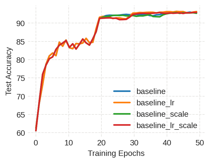
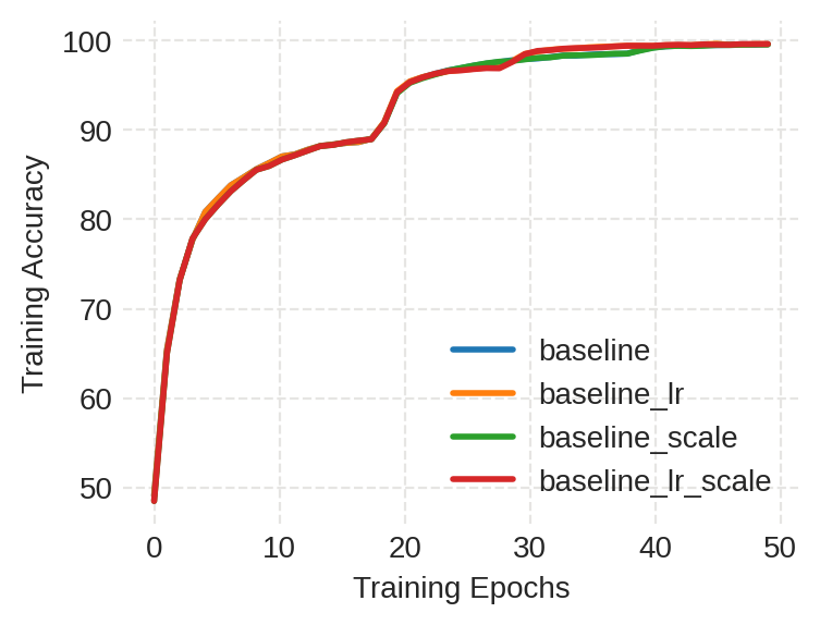
[Testing Accuracy] [Training Accuracy] [Training Loss]

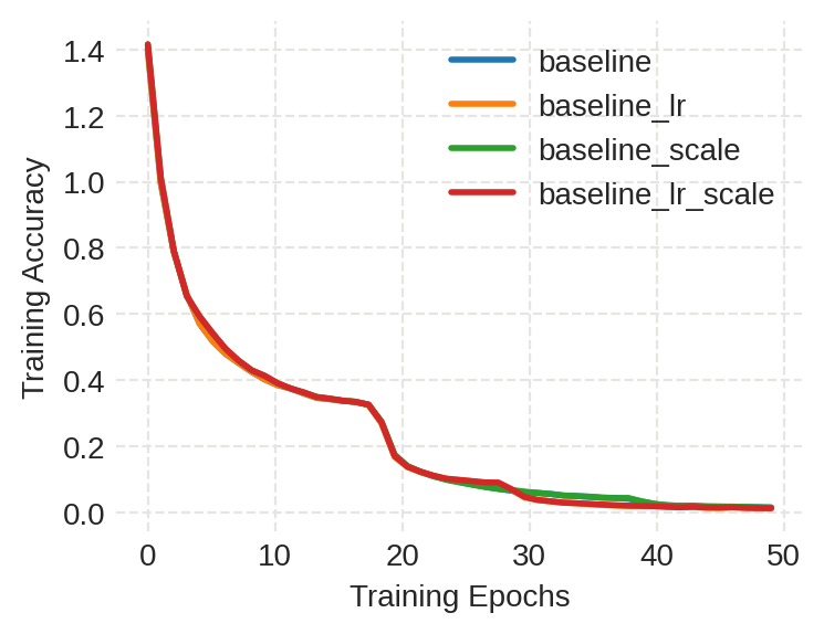
Figure 4: Training and testing behaviors of Amari’s Natural Gradient (baseline) on CIFAR-10. $baseline\_lr$ is the baseline method with the same learning rate scheduling as our method. $baseline\_scale$ is the baseline method with the same input scaling as our method. $baseline\_lr\_scale$ is the baseline method with the same learning rate scheduling and input scaling as our method.

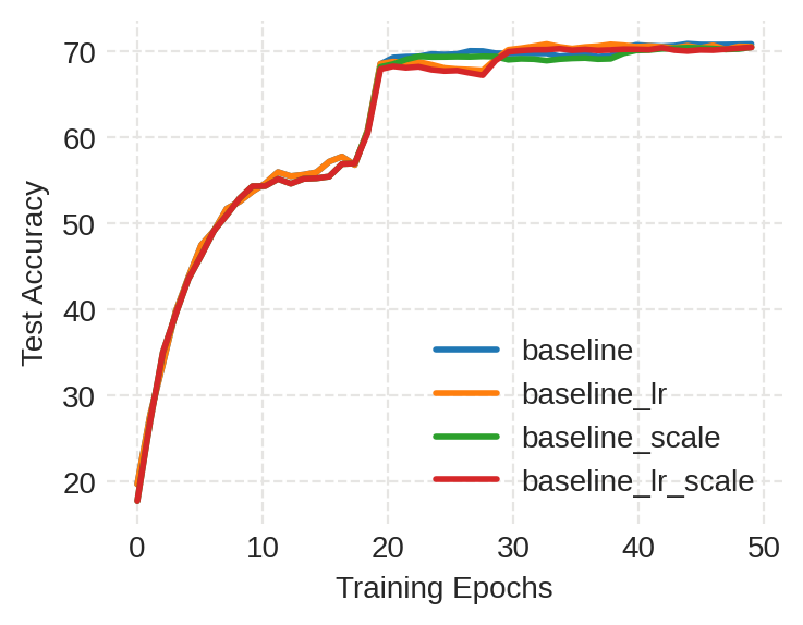
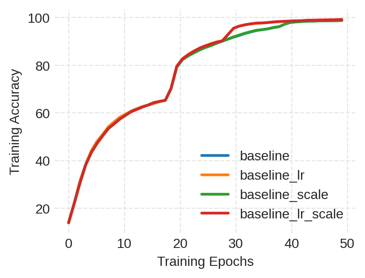
[Testing Accuracy] [Training Accuracy] [Training Loss]

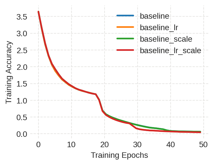
Figure 5: Training and testing behaviors Amari’s Natural Gradient (baseline) on CIFAR-100. $baseline\_lr$ is the baseline method with the same learning rate scheduling as our method. $baseline\_scale$ is the baseline method with the same input scaling as our method. $baseline\_lr\_scale$ is the baseline method with the same learning rate scheduling and input scaling as our method.

Appendix D The Pullback Metric on a Simple Neural Network

In this appendix, we compute the pullback metric for a two-layer neural network (NN). While we have argued that the pullback metric is the only natural metric, the complexity of the pullback metric motivates the simplifying assumptions in §6.

For a NN neural network with $\ell$ layers, specifically a feedforward neural networks where $\phi(w)$ is the composition of a sequence of layer functions, we have $W=W_{1}\times\ldots\times W_{\ell}$ in (1), where $W_{i}$ is the space of parameters for the $i^{\rm th}$ layer, ${\mathcal{M}}$ is the space of input to output functions, and $\phi(w)$ is the NN-specific function which assigns to input vector $x$ the NN output $y=\phi(w)(x).$ Passing between layers $L_{i}$ and $L_{i+1}$ consists of applying a matrix $A_{m_{i}\times n_{i}}$ and an activation function $f_{i}$. The number of parameters in $W_{i}$ is $m_{i}n_{i},$ under the assumption that $f_{i}$ does not depend on parameters.

For simplicity, we consider a two-layer neural network,

$$P_{1}:\leavevmode\hbox to132.6pt{\vbox to18.7pt{\text{[drawing]}}}\hskip 28.90755ptP_{2}:\leavevmode\hbox to134.15pt{\vbox to18.7pt{\text{[drawing]}}} {W_{1}} {{\rm Maps}(\mathbb{R}^{n},\mathbb{R}^{d})={\mathcal{M}}_{1}} \scriptstyle{\phi_{1}} {W_{2}} {{\rm Maps}(\mathbb{R}^{d},\mathbb{R}^{m})={\mathcal{M}}_{2}} \scriptstyle{\phi_{2}} {W_{1}} {{\rm Maps}(\mathbb{R}^{n},\mathbb{R}^{d})={\mathcal{M}}_{1}} \scriptstyle{\phi_{1}} {W_{2}} {{\rm Maps}(\mathbb{R}^{d},\mathbb{R}^{m})={\mathcal{M}}_{2}} \scriptstyle{\phi_{2}}$$ (40)

$$P_{T}:\leavevmode\hbox to135.71pt{\vbox to50.01pt{\text{[drawing]}}} {W_{1}\times W_{2}} {{\rm Maps}(\mathbb{R}^{n},\mathbb{R}^{m})} {\mathbb{R}} \scriptstyle{\phi_{NN}} \scriptstyle{\widetilde{F}_{NN}} \scriptstyle{F_{NN}} {W_{1}\times W_{2}} {{\rm Maps}(\mathbb{R}^{n},\mathbb{R}^{m})} {\mathbb{R}} \scriptstyle{\phi_{NN}} \scriptstyle{\widetilde{F}_{NN}} \scriptstyle{F_{NN}}$$

where

$$\phi_{NN}(w_{1},w_{2})=\phi_{2}(w_{2})\circ\phi_{1}(w_{1}).$$ (41)

Here we have absorbed the activation functions $f_{1},f_{2}$ into $\phi_{1},\phi_{2}$, respectively.

We now make (41) more explicit. For the first layer, we have a $d\times n$ matrix $(A_{w})_{i}^{j}$ depending on $w\in W_{1}$ and an activation function $f_{1}:\mathbb{R}\to\mathbb{R}.$ For $x\in\mathbb{R}^{n}$, define $\phi_{1}(w)(x)=f_{1}A_{w}(x)$, with $f_{1}$ acting componentwise of $A_{w}(x).$ Thus

$$\phi_{1}(w)(x)=\left(\begin{array}[]{c}f_{1}[(A_{w})_{1}^{j}x_{j}]\\ f_{1}[(A_{w})_{2}^{j}x_{j}]\\ \vdots\\ f_{1}[(A_{w})_{d}^{j}x_{j}]\end{array}\right)$$

with summation convention. We can write $\phi_{1}(w)(x)=[f_{1}\cdot{\rm Id}_{d}]\circ A_{w}(x)$, where ${\rm Id}_{d}$ is the $d\times d$ identity matrix, and $\circ$ is either composition or matrix multiplication. Dropping the identity matrix, for $f_{2}$ and $B_{w}$ defined for the second layer as above, (41) becomes

$$\phi_{NN}(w_{1},w_{2})(x)=(f_{2}\circ B_{w_{2}}\circ f_{1}\circ A_{w_{1}})(x).$$ (42)

We compute the pullback metric $\phi^{*}_{NN}\bar{g}$ for $\bar{g}$ the $L^{2}$ metric on ${\rm Maps}(\mathbb{R}^{n},\mathbb{R}^{m})$, even though we know this metric is too weak to produce a gradient. The $L^{2}$ metric is

$$\langle h_{1},h_{2}\rangle_{L^{2}}=\sum_{k=1}^{m}\int_{\mathbb{R}^{n}}h_{1}^{k}(x)h_{2}^{k}(x)dx,$$

where $h_{i}(x)=(h_{i}^{1}(x),\ldots,h_{i}^{m}(x)).$ In our case, $\phi_{NN}(W_{1}\times W_{2})$ consists of matrices, so tangent vectors to $\phi_{NN}(W_{1}\times W_{2})$ are again matrices. In particular, if $h_{1}=C^{j}_{i},h_{2}=D_{i}^{j}$ are $m\times n$ matrices, then $\langle h_{1},h_{2}\rangle_{L^{2}}=\int_{\mathbb{R}^{n}}{\rm Tr}(CD^{T})dx.$

Since $\phi_{2}(w_{2})$ is an $m\times d$ matrix, we can write $W_{2}=\{(w_{2,a}^{b}):1\leq a\leq d,1\leq b\leq m\}$, $(B_{w_{2},j}^{i})=(b^{i}_{j}(w_{2,j}^{i})),$ and similarly for $W_{1}$ and $A=(a_{c}^{d}(w_{1,c}^{d})$. Using $(\partial/\partial w_{2,r}^{s})B=(\delta_{r}^{s}(b_{r}^{s})^{\prime})$ (with no sum over $r,s$), we get

$$\frac{\partial\phi_{NN}}{\partial w_{2,r}^{s}}\biggl{|}_{(w_{1}^{0},w_{2}^{0})}(x) =f_{2}^{\prime}((B_{w_{2}^{0}}\circ f_{1}\circ A_{w_{1}^{0}})(x))\left(0,\cdots,0,(b_{r}^{s})^{\prime}(f_{1}\circ A_{w_{1}^{0}}(x))x_{s},0,\cdots,0\right)^{T}$$ (43)

with the nonzero entry in the last vector in the $s^{\rm th}$ slot. Also,

$$\frac{\partial\phi_{NN}}{\partial w_{1,c}^{d}}\biggl{|}_{(w_{1}^{0},w_{2}^{0})}(x) =f_{2}^{\prime}((B_{w_{2}^{0}}\circ f_{1}\circ A_{w_{1}^{0}})(x))\circ B_{w_{2}^{0}}((f_{1}\circ A_{w_{1}^{0}})(x))\circ f_{1}^{\prime}(A_{w_{1}^{0}}(x))$$

$$\qquad\circ\left(0,\cdots,0,(a_{c}^{d})^{\prime}(x)x_{d},0,\cdots,0\right)^{T},$$ (44)

with the nonzero entry in the $d^{\rm th}$ slot.

This gives an explicit expression for the pullback metric $(\phi^{*}\bar{g})$. For example, the $(\phi^{*}\bar{g})_{ij}$ component with $i=(1,c,d),j=(2,r,s)$ corresponding to directions in $W_{1},W_{2}$, respectively, is

$$(\phi^{*}_{NN}\bar{g})_{(1,c,d),(2,s,r)}(w_{1}^{0},w_{2}^{0})=\left\langle\frac{\partial\phi_{NN}}{\partial w_{1,c}^{d}},\frac{\partial\phi_{NN}}{\partial w_{2,r}^{s}}\right\rangle_{L^{2},\phi_{NN}(w_{1}^{0},w_{2}^{0})}$$

$$=\int_{\mathbb{R}^{n}}{\rm Tr}\left(\left[\frac{\partial\phi_{NN}}{\partial w_{1,c}^{d}}\biggl{|}_{(w_{1}^{0},w_{2}^{0})}(x)\right]\left[\frac{\partial\phi_{NN}}{\partial w_{2,r}^{s}}\biggl{|}_{(w_{1}^{0},w_{2}^{0})}(x)\right]^{T}\right)dx,$$

where we have to plug (43, D) into the right hand side. There are similar expressions for other components of the metric tensor.

Even in the simplest case ${\rm dim}(W_{1})={\rm dim}(W_{2})=m=n=1$, we do not get that the pullback metric is a $2\times 2$ matrix consisting of two $1\times 1$ blocks, because we cannot expect

$$\left\langle\frac{\partial}{\partial w_{1}},\frac{\partial}{\partial w_{2}}\right\rangle_{\phi^{*}\bar{g},(w_{1}^{0},w_{2}^{0})} =\left\langle\frac{\partial\phi_{NN}}{\partial w_{1}},\frac{\partial\phi_{NN}}{\partial w_{2}}\right\rangle_{L^{2},\phi_{NN}(w_{1}^{0},w_{2}^{0})}$$

$$=\int_{\mathbb{R}}[f_{2}^{\prime}(b_{w_{2}^{0}}\cdot f_{1}(a_{w_{1}^{0}z}(x)))\cdot b_{w_{2}^{0}}^{\prime}(f_{1}(a_{w_{1}^{0}}(x)))x]$$

$$\qquad\cdot[f_{2}^{\prime}(b_{w_{2}^{0}}\cdot f_{1}(a_{w_{1}^{0}z}(x)))\cdot b_{w_{2}^{0}}(f_{1}(a_{w_{1}^{0}}(x)))\cdot f_{1}^{\prime}(a_{w_{1}^{0}}x)\cdot a_{w_{1}^{0}}^{\prime}(x)]\ dx$$

to be zero. Thus some sort of simplifying assumptions as in §6 are necessary.

Appendix E Riemannian Primal and Mirror Descent

There is a large literature devoted to convex optimization, and empirical loss functions $\ell:{\mathcal{M}}\to\mathbb{R}$ in (1) are often chosen to be convex. However, the induced loss function $\ell\circ\phi:W\to\mathbb{R}$ on the parametri space $W$ may no longer be convex. In this section, we assume that $\ell\circ\phi$ is still convex, and study how the primal and mirror descent from (Allen-Zhu and Orecchia, 2014) carries over to the manifold (possible with boundary) $W$ with the pullback metric. In any case, these techniques can be applied on a region where $\ell\circ\phi$ is convex, specifically in neighborhoods of a local minimum which contain no other critical points. In addition, in overparametrized situations, non-convex problems often behave like convex problems (Arora et al., 2019).

As in (Allen-Zhu and Orecchia, 2014), consider a convex function $f$ defined on an open convex set $Q\subset\mathbb{R}^{n}$ and satisfying the ${\mathbb{E}}$-Lipschitz condition:

$$\exists L>0\ {\rm such\ that}\ \forall x,y\in Q,\ \|\nabla f(x)-\nabla f(y)\|_{E}\leq L\|x-y\|_{E}.$$ (45)

Here the subscript $E$ denotes the Euclidean norm, and the gradient is the usual Euclidean gradient. Then we have

$$\forall y,\ \ f(y)\leq f(x)+\langle\nabla f(x),y-x\rangle_{E}+\frac{L}{2}\|y-x\|^{2}_{E}.$$ (46)

Here all norms, inner products, and gradients are with respect to the usual dot product on $\mathbb{R}^{n}.$

If $Q$ has some other Riemannian metric $g$, which for us is typically the pullback metric from a mapping space, then

$$\langle\nabla f(x),y-x\rangle_{E}=df_{x}(y-x)=\langle\nabla^{g}f(x),y-x\rangle_{g,x},$$ (47)

by the characterization of the gradient $\nabla^{g}f.$ Note that in the last term, we consider $y-x$ to be in $T_{x}Q$, which is acceptable since $Q\subset\mathbb{R}^{n}.$ Thus (46) trivially becomes

$$\forall y,\ \ f(y)\leq f(x)+\langle\nabla^{g}f(x),y-x\rangle_{g,x}+\frac{L}{2}\|y-x\|^{2}_{E}.$$ (48)

Since (48) still depends on Euclidean norm, we introduce the following assumption on $g$ to get a Riemannian version of (48).

Definition E.1.

A Riemannian metric $g$ on $Q$ is ${\mathbb{E}}$-compatible if there exists $C>0$ such that for all $x,y\in Q$,

$$\|x-y\|_{E}\leq C^{1/2}\|x-y\|_{g,x}.$$ (49)

This condition is of course satisfied if $Q$ is compact. The hyperbolic metric on $\mathbb{H}^{n}$ is not ${\mathbb{E}}$-compatible, but the hyperbolic metric on the noncompact convex set $\mathbb{R}^{n-1}\times(0,A]$ is ${\mathbb{E}}$-compatible for any $A.$

By (48) and (49), we have

$$f(y) \leq f(x)+\langle\nabla f(x),y-x\rangle_{g,x}+\frac{L}{2}\|y-x\|^{2}_{E}$$

$$\leq f(x)+\langle\nabla^{g}f(x),y-x\rangle_{g,x}+\frac{CL}{2}\|y-x\|^{2}_{g,x}.$$ (50)

E.1 Gradient descent guarantee

From this point on, we use $\nabla f(x)$ and $\nabla f_{x}$ interchangeably. Based on (E), we make the following definition:

Definition E.2.

$${\bf Grad}(x) ={\rm argmin}_{y\in Q}\left(\langle\nabla^{g}f_{x},y-x\rangle_{g,x}+\frac{CL}{2}\|y-x\|^{2}_{g,x}\right),$$

$${\bf Prog}(x) =-\min_{y\in Q}\left(\langle\nabla^{g}f_{x},y-x\rangle_{g,x}+\frac{CL}{2}\|y-x\|^{2}_{g,x}\right).$$

Lemma E.3.

For $Q=\mathbb{R}^{n}$, we have

$${\bf Grad}(x)=x-\frac{1}{CL}\nabla^{g}f(x),\ \ {\bf Prog}(x)=\frac{1}{2CL}\|\nabla^{g}f(x)\|_{g,x}^{2}.$$

This reproduces the Euclidean result if $g$ is the Euclidean metric (as then $C=1$).

Proof E.4.

At ${\bf Grad}(x)=y$, we have, for all $k$,

$$0 =\partial_{y^{k}}\left(\langle\nabla^{g}f_{x},y-x\rangle_{g,x}+\frac{CL}{2}\|y-x\|^{2}_{g,x}\right)$$

$$=\partial_{y^{k}}\langle\nabla f_{x},y-x\rangle_{E}+\frac{CL}{2}\partial_{y^{k}}(g_{ij}(x)(y-x)^{i}(y-x)^{j})$$

$$=\partial_{y^{k}}\left(\frac{\partial f}{\partial y^{i}}(x)(y-x)^{i}\right)+\frac{CL}{2}g_{kj}(x)[2y^{j}-2x^{j}]$$

$$=\frac{\partial f}{\partial y^{k}}(x)+CL\cdot g_{kj}(x)[2y^{j}-2x^{j}].$$

Thus the components of $y$ satisfy

$$0=g^{ki}\left(\frac{\partial f}{\partial y^{k}}(x)+CL\cdot g_{kj}(x)[2y^{j}-2x^{j}]\right)=(\nabla^{g}f(x))^{i}+CLy^{i}-CLx^{i},$$

for all $i$. This gives

$$y=x-\frac{1}{CL}\nabla^{g}f(x).$$

Plugging this into the definition of Prog$(x)$ finishes the proof.

Now we can get the Riemannian analogue of the estimate of primal guarantee.

Corollary E.5.

For $Q=\mathbb{R}^{n}$, assume that $f$ is ${\mathbb{E}}$-Lipschitz with constant $L$ and that $g$ is ${\mathbb{E}}$-compatible with constant $C$. Then the algorithm $x_{k+1}\leftarrow x_{k}-\frac{1}{CL}\nabla^{g}f(x_{k})$ satisfies

$$f(x_{k})-f(x_{k+1})\geq\frac{1}{2CL}\|\nabla^{g}f(x_{k})\|_{g,x_{k}}^{2}.$$

Proof E.6.

Since $x_{k+1}={\bf Grad}(x_{k})$, we have

$$f(x_{k+1})\leq f(x_{k})+\langle\nabla^{g}f_{x_{k}},x_{k+1}-x_{k}\rangle_{g,x_{k}}+\frac{CL}{2}\|x_{k+1}-x_{k}\|^{2}_{g,x_{k}}\leq f(x_{k})-\frac{1}{2CL}\|\nabla^{g}f(x_{k})\|_{g,x_{k}}^{2}.$$

Note that the progress is good if $\|\nabla^{g}f\|_{g,x}$ is large.

Corollary E.7.

For general $Q$, under the hypotheses of the previous Corollary, we have

$$f(x_{k})-f(x_{k+1})\geq{\bf Prog}(x_{k}).$$

The proof is the same as the previous Corollary.

Lemma E.8.

Let $f$ be a ${\mathbb{E}}$-Lipschitz with constant $L$ on $Q=\mathbb{R}^{n}$ and $g$ is ${\mathbb{E}}$-compatible with constant $C$. For any initial point $x_{0}\in Q$, consider $T$ steps of ${\bf Grad}(x)$, then the last point $x_{T}$ satisfies

$$f(x_{T})-f(x^{*})\leq O\left(\frac{LCR^{2}}{T}\right),$$

where $R=\max_{x:f(x)\leq f(x_{0})}\|x-x^{*}\|_{g}$, and $x^{*}$ is any minimizer of $f$.

Proof E.9.

By the convexity of $f$ and Cauchy-Schwartz, we have

$$f(x_{k})-f(x^{*}) \leq\langle\nabla f(x_{k}),x_{k}-x^{*}\rangle=\langle\nabla^{g}f(x_{k}),x_{k}-x^{*}\rangle_{g}\leq\|\nabla^{g}f(x_{k})\|_{g}\cdot\|x_{k}-x^{*}\|_{g}$$

$$\leq R\cdot\|\nabla^{g}f(x_{k})\|_{g}.$$

if $D_{k}=f(x_{k})-f(x^{*})$ denotes the distance to the optimum at iteration $k$, then $D_{k}\leq R\cdot\|\nabla^{g}f(x_{k})\|_{g}$. In addition, $D_{k}-D_{k+1}\geq\frac{1}{CL}\|\nabla^{g}f(x_{k})\|^{2}_{g,x_{k}}$ by Corollary E.5. Therefore,

$$D^{2}_{k}\leq 2LCR^{2}(D_{k}-D_{k+1})\Longrightarrow\frac{D_{k}}{D_{k+1}}\leq 2LCR^{2}\left(\frac{1}{D_{k+1}}-\frac{1}{D_{k}}\right).$$

We have $D_{k}\geq D_{k+1}$, since the objective decreases at each iteration, so $\left(\frac{1}{D_{k+1}}-\frac{1}{D_{k}}\right)\geq\frac{1}{2LCR^{2}}$. Telescoping through $T$ iterations, we have $\frac{1}{D_{T}}\geq\frac{T}{2LCR^{2}}$, i.e., $f(x_{T})-f(x^{*})\leq\frac{2LCR^{2}}{T}.$

E.2 Mirror descent Guarantee

We have just seen that the mirror descent algorithm has the same form for the Euclidean or Riemannian gradient. In contrast, using the relationship in (Raskutti and Mukherjee, 2015) between mirror descent and natural gradient, we can establish a new convergence result for mirror descent using the Riemannian (or natural) gradient descent guarantee established in §E.1.

Given a strongly convex distance generating function $w:Q\to\mathbb{R}$, the Bregman divergence is defined by

$$V_{x}(y)=w(y)-\langle\nabla w(x),y-x\rangle-w(x).$$ (51)

The mirror descent update with step size $\alpha$ is

$$x_{k+1}=\operatorname{argmin}_{y}\left\{\langle\nabla f(x_{k}),y-x_{k}\rangle+\alpha V_{x_{k}}(y)\right\}.$$

According to (Raskutti and Mukherjee, 2015, Theorem 1), this update is equivalent to the following Riemannian gradient descent step for the Riemannian manifold $(\Phi,\nabla^{2}H)$,

$$z_{k+1}=z_{k}-\frac{1}{\alpha}[\nabla^{2}H(z_{k})]^{-1}\nabla_{z}f(h(z)).$$ (52)

Here $\Phi:=\nabla w(Q)=\{\nabla_{w}(q):q\in Q\}$, and $H$ is the convex (or Fenchel) conjugate function of $w$,

$$H(z)=\sup_{x\in Q}\{\langle x,z\rangle-w(x)\}.$$ (53)

It is standard that $h=\nabla H$ is the inverse of $\nabla w.$

(52) can be rewritten as the following primal gradient descent for the pullback metric $g:=\nabla^{2}H$,

$$z_{k+1}=z_{k}-\frac{1}{\alpha}\nabla^{g}F(z),$$ (54)

where $F=f\circ h$. If $F$ is ${\mathbb{E}}$-Lipschitz with constant $L=L_{F}$ and $\nabla^{2}H$ is ${\mathbb{E}}$-compatible with constant $C=C_{F}$, then for $\alpha=CL$, Corollary E.5 gives

$$F(z_{k})-F(z_{k+1})\geq\frac{1}{2CL}\|\nabla^{g}F(z_{k})\|_{g,z_{k}}^{2}.$$

For $T$ iterations of such gradient steps, by Lemma E.8,

$$F(z_{T})-F(z^{*})\leq O\left(\frac{LCR^{2}}{T}\right).$$

We now compute some examples. Recall that for $w(x)=\frac{1}{2}\|x\|_{E}^{2}$, we get $H(z)=\frac{1}{2}\|z\|_{E}^{2}$, so $\nabla^{2}H$ is just the Euclidean metric; i.e., mirror descent for this $w$ is just Euclidean gradient descent.

To relate $w$ to a Riemannian metric $g$, e.g., a pullback metric, we fix $a\in W$ and set $w^{a}(x)=\frac{1}{2}\|x\|_{g(a)}^{2}.$ As in the Euclidean case, it is straightforward to check that $w^{a}$ is strongly convex with parameter $1$:

$$\frac{1}{2}\|tx+(1-t)y\|_{g(a)}^{2} =\frac{1}{2}g_{ij}(a)(tx+(1-t)y)^{i}(tx+(1-t)y)^{j}$$

$$=\frac{1}{2}g_{ij}(a)(t^{2}x^{i}x^{j}+2t(1-t)x^{i}y^{j}+(1-t)^{2}y^{i}y^{j})$$

$$=\frac{1}{2}\left(tg_{ij}(a)x^{i}x^{j}+(1-t)g_{ij}(a)y^{i}y^{j}-t(1-t)g_{ij}(a)(x^{i}x^{j}-2x^{i}y^{j}+y^{i}y^{j})\right)$$

$$=\frac{1}{2}\left(t\|x\|_{g(a)}^{2}+(1-t)\|y\|_{g(a)}^{2}-t(1-t)\|x-y\|_{g(a)}^{2}\right)$$

The Bregman divergence associated to $w^{a}$ is

$$V^{a}_{x}(y) =V^{g}_{x}(y)=\frac{1}{2}\left(\|y\|^{2}_{g(a)}-\|x\|_{g(a)}^{2}-\langle\nabla^{E}\|x\|_{g(a)}^{2},y-x\rangle_{E}\right)$$

$$=\frac{1}{2}\left(\|y\|^{2}_{g(a)}-\|x\|_{g(a)}\partial_{j}\|x\|_{g(a)}\cdot(y-x)^{j}\right)$$

$$=\frac{1}{2}\left(\|y\|^{2}_{g(a)}-\|x\|_{g(a)}^{2}-\partial_{j}(g_{rs}(a)x^{r}x^{s})(y-x)^{j}\right)$$

$$=\frac{1}{2}\left(\|y\|^{2}_{g(a)}-\|x\|_{g(a)}^{2}-2g_{js}(a)x^{s}(y-x)^{j}\right)$$

$$=\frac{1}{2}\left(\|y\|^{2}_{g(a)}-\|x\|_{g(a)}^{2}+2\|x\|_{g(a)}^{2}-2\langle x,y\rangle_{g(a)}\right)$$

$$=\frac{1}{2}\|x-y\|^{2}_{g(a)}.$$

Therefore, the mirror descent update for $w^{a}$ is

$$x_{k+1} =\operatorname{argmin}_{y}\left\{\langle\nabla^{E}f(x_{k}),y-x_{k}\rangle+\frac{\alpha}{2}\|x_{k}-y\|^{2}_{g(a)}\right\}.$$

Recall that $\langle\nabla^{E}f(x_{k}),y-x_{k}\rangle_{E}=\langle\nabla^{g}f(x_{k}),y-x_{k}\rangle_{g(b)}$ for any $b\in\Phi.$ Since $\nabla^{g}f$ is evaluated at $x_{k}$, it makes the most sense to set $b=x_{k}.$ Thus the mirror descent update becomes

$$x_{k+1} =\operatorname{argmin}_{y}\left\{\langle\nabla^{E}f(x_{k}),y-x_{k}\rangle+\frac{\alpha}{2}\|x_{k}-y\|^{2}_{g(x_{k})}\right\}$$ (55)

$$=\operatorname{argmin}_{y}\left\{\langle\nabla^{g}f(x_{k}),y-x_{k}\rangle_{g(x_{k})}+\frac{\alpha}{2}\|x_{k}-y\|^{2}_{g(x_{k})}\right\}.$$

We now find this argmin. In the next calculation, $g=g(x_{k}),g_{rs}=g_{rs}(x_{k})$, etc. We must solve

$$0 =\frac{\partial}{\partial y^{i}}\left(\langle\nabla^{g}f(x_{k}),y-x_{k}\rangle_{g}+\frac{\alpha}{2}\|x_{k}-y\|^{2}_{g}\right)$$

$$=\frac{\partial}{\partial y^{i}}\left(g_{rs}(g^{ar}\partial_{a}f(x_{k}))\cdot(y-x)^{s}+\frac{\alpha}{2}g_{rs}(x_{k}-y)^{r}(x_{k}-y)^{s}\right)$$

$$=\partial_{i}f(x_{k})-\alpha\cdot g_{ri}(x_{k}-y)^{r},$$

since in the last term on the second line, $(\partial/\partial y^{i})g_{rs}(x_{k})=0.$ Thus the argmin $y=x_{k+1}$ satisfies

$$g_{ri}y^{r} =g_{ri}x_{k}^{r}-\frac{1}{\alpha}\partial_{i}f(x_{k})\Rightarrow g^{ai}g_{ri}y^{r}=g^{ai}g_{ri}x_{k}^{r}-\frac{1}{\alpha}g^{ai}\partial_{i}f(x_{k})\Rightarrow y^{a}=x_{k}^{a}-\frac{1}{\alpha}g^{ai}\partial_{i}f(x_{k})$$

$$\Rightarrow y=x_{k}-\frac{1}{\alpha}\nabla^{g}f(x_{k})\Rightarrow y=x_{k}-\frac{1}{\alpha}\nabla^{g}f(x_{k}).$$

In other words, the mirror descent update is

$$x_{k+1}=x_{k}-\frac{1}{\alpha}\nabla^{g}f(x_{k}).$$ (56)

This gives a Riemannian version of mirror descent.

Proposition E.10.

Mirror descent of step size $\alpha$ associated to the function $f$ and with distance generating function $w^{x_{k}}(y)=\frac{1}{2}\|x-y\|_{g(x_{k})}^{2}$ at the k^th step is equivalent to natural gradient descent of $f$ with step size $1/\alpha$.

As a final remark, it is easy determine $H_{a}(z):=\sup_{x\in Q}\{\langle x,z\rangle_{g(a)}-w_{a}(x)\}$. In fact,

$$0=\frac{\partial}{\partial x^{i}}\left(g_{rs}(a)x^{r}z^{s}-\frac{1}{2}g_{rs}(a)x^{r}x^{s}\right)\Rightarrow 0=g_{is}(a)z^{s}-g_{is}(a)x^{s}\Rightarrow z=x,$$

so $H_{a}(z)=\frac{1}{2}\|z\|_{g(a)}^{2}$. Then $\nabla^{2}_{E,a}H_{a}=(g_{ij}(a))$, i.e. $\nabla^{2}_{E,a}H_{a}=g(a).$ However, $\nabla^{2}_{g,a}H_{a}$ is more complicated.

References

- Allen-Zhu and Orecchia (2014) Zeyuan Allen-Zhu and Lorenzo Orecchia. Linear coupling: An ultimate unification of gradient and mirror descent. arXiv preprint arXiv:1407.1537, 2014.
- Amari (1998) Shun-Ichi Amari. Natural gradient works efficiently in learning. Neural computation, 10(2):251–276, 1998.
- Arora et al. (2019) Sanjeeva Arora, Simon S. Du, Wei Hu, Zhiyuan Li, Rusian Salakhutdinov, and Ruosong Wang. On exact computation with an infinitely wide neural net. arXiv preprint arXiv:1904:11955, 2019.
- Benjamin et al. (2019) Ari Benjamin, David Rolnick, and Konrad Kording. Measuring and regularizing networks in function space. In International Conference on Learning Representations, 2019.
- Chizat et al. (2019) Lénaïc Chizat, Edouard Oyallon, and Francis Bach. On lazy training in differentiable programming. arXiv preprint arXiv:1812.07956, 2019.
- Dieuleveut et al. (2016) Aymeric Dieuleveut, Francis Bach, et al. Nonparametric stochastic approximation with large step-sizes. Annals of Statistics, 44(4):1363–1399, 2016.
- Dinh et al. (2017) Laurent Dinh, Razvan Pascanu, Samy Bengio, and Joshua Bengio. Sharp minima can generalize for deep nets. arXiv preprint arXiv:1703.04933, 2017.
- Gilkey (1995) Peter B. Gilkey. Invariance theory, the heat equation, and the Atiyah-Singer index theorem. Studies in Advanced Mathematics. CRC Press, Boca Raton, FL, second edition, 1995.
- Grosse and Martens (2016) Roger Grosse and James Martens. A kronecker-factored approximate fisher matrix for convolution layers. In International Conference on Machine Learning, pages 573–582. PMLR, 2016.
- Jacot et al. (2019) Arthur Jacot, Franck Gabriel, and Clément Hongler. Neural tangent kernel: Convergence and generalization in neural networks. arXiv preprint arXiv:1806.07572, 2019.
- Kakade (2001) Sham M Kakade. A natural policy gradient. Advances in neural information processing systems, 14, 2001.
- Martens (2014) James Martens. New insights and perspectives on the natural gradient method. arXiv preprint arXiv:1412.1193, 2014.
- Martens and Grosse (2015) James Martens and Roger Grosse. Optimizing neural networks with kronecker-factored approximate curvature. In International conference on machine learning, pages 2408–2417. PMLR, 2015.
- Ollivier (2015) Yann Ollivier. Riemannian metrics for neural networks i: Feedforward networks. Information and Inference: A Journal of the IMA, 4(2):108–153, 2015.
- Pascanu and Bengio (2013) Razvan Pascanu and Yoshua Bengio. Revisiting natural gradient for deep networks. arXiv preprint arXiv:1301.3584, 2013.
- Raskutti and Mukherjee (2015) Garvesh Raskutti and Sayan Mukherjee. The information geometry of mirror descent. IEEE Transactions on Information Theory, 61(3):1451–1457, 2015.
- Rosenberg (1997) Steven Rosenberg. The Laplacian on a Riemannian manifold: An introduction to analysis on manifolds. Cambridge University Press, Cambridge, 1997.
- Wang (2019) Chaoqi Wang. https://github.com/alecwangcq/KFAC-Pytorch. 2019.
- Watson (1922) G. N. Watson. A treatise on the theory of Bessel functions. Cambridge University Press, London, 1922.
- Wendland (2004) Holger Wendland. Scattered data approximation, volume 17. Cambridge University Press, London, 2004.
- Zhang et al. (2019a) Guodong Zhang, Lala Li, Zachary Nado, James Martens, Sushant Sachdeva, George Dahl, Chris Shallue, and Roger B Grosse. Which algorithmic choices matter at which batch sizes? insights from a noisy quadratic model. Advances in neural information processing systems, 32, 2019a.
- Zhang et al. (2019b) Guodong Zhang, James Martens, and Roger B Grosse. Fast convergence of natural gradient descent for over-parameterized neural networks. Advances in Neural Information Processing Systems, 32, 2019b.
- Zhang et al. (2019c) Guodong Zhang, Chaoqi Wang, Bowen Xu, and Roger Grosse. Three mechanisms of weight decay regularization. In International Conference on Learning Representations, 2019c.