Panoramic mapping of phonon transport from ultrafast electron diffraction and machine learning

Abstract

One central challenge in understanding phonon thermal transport is a lack of experimental tools to investigate mode-based transport information. Although recent advances in computation lead to mode-based information, it is hindered by unknown defects in bulk region and at interfaces. Here we present a framework that can reveal microscopic phonon transport information in heterostructures, integrating state-of-the-art ultrafast electron diffraction (UED) with advanced scientific machine learning. Taking advantage of the dual temporal and reciprocal-space resolution in UED, we are able to reliably recover the frequency-dependent interfacial transmittance with possible extension to frequency-dependent relaxation times of the heterostructure. This enables a direct reconstruction of real-space, real-time, frequency-resolved phonon dynamics across an interface. Our work provides a new pathway to experimentally probe phonon transport mechanisms with unprecedented details.

The ability to efficiently transport, convert, and store thermal energy plays an indispensable role in promoting decarbonization and mitigating global warming ^{henry2020five}. Significant efforts have been directed to understand thermal transport at the nanoscale ^{cahill2014nanoscale} driven by applications such as thermoelectric energy harvesting ^{Minnich2009Review}, heat management in microelectronics ^{moore2014emerging}, high-efficiency thermal storage systems ^{amaral2017storage}, and passive cooling of structural materials ^{li2019radiative}. However, our understanding of phonon thermal transport is largely hindered by the lack of experimental tool that can resolve mode-based phonon transport, both in the bulk region and across interfaces. Observables like heat capacity and thermal conductivity are mode- or frequency-integrated. Although computation can resolve phonon transport modal information such as interface transmittance and mean-free-paths, it relies heavily on detailed atomic and defect configurations that are usually unknown. Here, we present an integrated experimental-computational-machine learning framework that can resolve frequency-dependent phonon interfacial transmittance and phonon relaxation times using a laser-pump, electron-probe ultrafast electron diffraction (UED) setup. The acquired information offers unprecedentedly detailed knowledge on phonon transport, enabling new understanding that will have both fundamental and practical importance.

In the past two decades, remarkable progress has been made in understanding phonon thermal transport, enabled by advances in experimental and computational techniques ^{cahill2004analysis, broido2007intrinsic, Schmidt2008tdtr, lindsay2013phononisotope, regner2013broadband, Hu2015mfp, hua2017experimental, Maznev2011nondiff, ravichandran2018spectrally, forghani2019phonon}. Novel phonon transport regimes have been observed^{chen2021non-fourier, qian2021phonon}, such as quantized, ballistic phonon transport ^{schwab2000measurement}, coherent phonon transport ^{Luckyanova2012coherent}, phonon Anderson localization ^{luckyanova2018phonon}, and hydrodynamic phonon transport ^{Huberman2019science, Machida2020Science}. On the other hand, a few works have demonstrated the power of using electron and x-ray diffraction to study phonon spectroscopy^{trigo2010imaging, zhu2015phonon, yan2021single-defect}, suggesting that diffraction techniques may also serve as powerful tools to study frequency-dependent phonon transport. However, these techniques are limited to bulk crystalline materials. Frequency-resolved interfacial transport remains a major challenge.

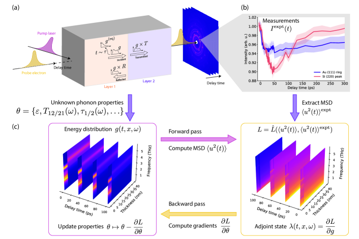
Figure 1: Workflow for learning phonon transport properties from ultrafast electron diffraction. (a) Illustration of a UED experiment on a two-layer heterostructure. A fs pump laser generates a thermal excitation, while ultrafast electrons generate the time-dependent diffraction patterns at a sequence of delay times $t$. (b) Representative measurements of $t$-dependent relative diffraction intensities of the two layers, which can be used to extract mean-squared displacements (MSD) $\langle u^{2}(t)\rangle^{\mathrm{expt}}$ through the atomic thermal motions from the Debye-Waller factor. (c) Illustration of the iterative algorithm used to learn phonon transport properties $\theta$. The phonon energy distribution $g(t,x,\omega)$ is calculated using the Boltzmann transport equation (BTE) with an initial guess for $\theta$ (which is a set of unknown phonon properties, such as phenomenological energy loss coefficients $\varepsilon_{1/2}$, frequency-dependent interfacial transmittance $T_{12/21}(\omega)$, and frequency-dependent relaxation times $\tau_{1/2}(\omega)$), and is then used to computationally obtain the MSDs $\langle u^{2}(t)\rangle$. The discrepancies between $\langle u^{2}(t)\rangle$ and the target, $\langle u^{2}(t)\rangle^{\mathrm{target}}=\langle u^{2}(t)\rangle^{\mathrm{expt}}$ here, are measured by a loss function $L$. The parameter gradients $\partial L/\partial\theta$ are obtained by the adjoint-state method and fed into an optimizer to minimize $L$ and provide improved estimates of $\theta$.

The UED measures the time-dependent diffraction patterns of each layer in a heterostructure with sub-ps resolution (Fig. 1(a)). Although the diffraction intensities in principle are linked to the atomic displacements through microscopic phonon transport and local temperature variations, the inverse problem of extracting phonon transport information, such as interfacial transmittance $T_{12/21}(\omega)$, and relaxation times $\tau_{1/2}(\omega)$ from time resolved diffraction information is difficult. The difficulties mainly originate from the high-dimensional phonon dynamics that depend on time, space, and frequency, and low-dimensional observables that are only time-dependent, and layer-specific diffraction patterns contain integrated information from all atoms in the domain. Given the advances in ab initio phonon computations^{minnich2015advances}, we consider some basic phonon properties such as density-of-states (DOS) and group velocities in each layer are known, and assume that the diffraction intensity smear comes solely from the lattice contributions after full electron thermalization. A number of key thermal transport parameters appeared in Boltzmann transport equation (BTE) can be reconstructed using advanced ajoint-state ^{cao2003adjoint} and automatic differentiation machine learning techniques ^{baydin2018automatic}, including frequency-dependent phonon transmittance across interface, with possible extension to frequency-dependent relaxation times, thereby is termed “panoramic mapping”. The machine learning techniques play a crucial role to reliably output high-dimensional frequency-dependent thermal transport information from diffraction spots’ time evolution. Since interfaces often play a key role in thermal transport, the unprecedentedly detailed knowledge of interfacial transport could lead to various applications including enhancement of heat transfer through interfacial engineering, development of high thermal conductivity materials for improved heat transfer, and materials and architectures design for thermal energy storage.

The framework setup

The overall architecture of the framework leading to panoramic phonon transport mapping is summarized in Fig. 1. First, we employ MeV-UED to acquire the time-resolved electron diffraction patterns of a heterostructure after the fs-laser excitation (pump laser) with transmission geometry (Fig. 1(a))^{weathersby2015mega, shen2018femtosecond}. Diffraction spots coming from different layers in a heterostructure system offer a natural layer-resolved information. Consider an Au/Si heterostructure used in experiments, the intensity evolution of the (111) ring in poly-crystalline Au and the (220) diffraction spot in single-crystalline Si are shown in Fig. 1(b) as an illustration. Our goal is to use such time-dependent diffraction information to extract the phonon transport properties. The key challenge is that diffraction results from contribution of all atoms in the layer while phonon transport depends on both time and space. Using the diffraction information of both layers in reciprocal space increases the reliability for information extraction. The Debye-Waller factor links the diffraction intensity $I(t)$ to the mean-squared atomic displacements (MSD) $\langle u^{2}(t)\rangle$ as $I(t)\propto\exp(-\frac{1}{3}q^{2}\langle u^{2}(t)\rangle)$ ($q=|\mathbf{q}|$ is the norm of the electron-beam wavevector transfer, $\langle\ldots\rangle$ indicates an ensemble average over atoms) at each time $t$. By feeding a set of generic phonon transport properties $\theta$ (e.g. transmittance), $\langle u^{2}(t)\rangle$ is directly computable from BTE, i.e., each $\langle u^{2}(t)\rangle$ time-series are labeled by parameters $\theta$. To extract the phonon transport from a target data of thickness-averaged MSD $\langle u^{2}(t)\rangle^{\mathrm{target}}$, which can come from real experimental data, we solve an optimization problem by minimizing the mean absolute loss $L=\frac{1}{N}\sum_{n=1}^{N}|\langle u^{2}(t_{n})\rangle-\langle u^{2}(t_{n})\rangle^{\mathrm{target}}|$ between the computed and experimentally extracted MSDs.

The entire process of minimizing loss function $L$ and extracting phonon properties $\theta$ is composed of two parts, the forward pass and the backward pass (Fig. 1(c)). In the forward pass, we simulate the MSD $\langle u^{2}(t)\rangle$ given an initial guess of the parameters $\theta$; the theoretical framework is visualized in Fig. 2(a). The time-dependent local MSD $\langle u^{2}(t,x)\rangle$ is directly linked to the phonon energy distribution $g(t,x,\omega)$ as ^{als2011elements}

$$\langle u^{2}(t,x)\rangle=\frac{1}{Nm}\int_{0}^{\infty}\frac{1}{\omega^{2}}\left(g(t,x,\omega)+\frac{\hbar\omega}{2}D(\omega)\right)\ \mathrm{d}\omega,$$ (1)

where $D(\omega)$, $N$, and $m$ are the phonon DOS, number of atoms per unit cell, and the atomic mass for monoatomic solid, respectively (a more general formulation is provided in Supplementary Information LABEL:SI_sec:DW_MSDs). The measured displacements $\langle u^{2}(t)\rangle$ from UED is the thickness-averaged displacement, that $\langle u^{2}(t)\rangle=\frac{1}{L}\int_{0}^{L}\langle u^{2}(t,x)\rangle\ \mathrm{d}x$ due to the transmission geometry. Due to the much larger spot size of the pump laser ($300\,\mathrm{\mu m}$ full width at half maximum, FWHM) compared to that of the probe electron ($100\,\mathrm{\mu m}$ FWHM), the changing diffraction intensities can be attributed to the cross-plane phonon transport process, which can be well captured by a one-dimensional BTE under the relaxation time approximation (RTA), that

$$\begin{split}\frac{\partial g(t,x,\omega)}{\partial t}&+\mu v(\omega)\frac{\partial g(t,x,\omega)}{\partial x}=\\ &-\frac{g(t,x,\omega)-g^{\mathrm{eq}}(T(t,x),\omega)}{\tau(\omega)},\end{split}$$ (2)

where $v(\omega)$ and $\tau(\omega)$ denote the frequency-dependent group velocities and relaxation times, respectively, and $\mu=\cos(\varphi)$ projects the group velocity at an angle $\varphi\in[0,\pi]$ to the $x$-direction (Fig. 2(a)).

The phonon transport across the interface is dictated by transmittance. For example, only partial energy of the right-propagating phonon in layer 1, $0\leq T_{12}(\omega)\leq 1$, gets transmitted to layer 2 while the rest get reflected, as illustrated in Fig. 2(a). The energy exchange rate between the phonon system and the environment is phenomenologically parameterized by $\varepsilon$ ($0\leq\varepsilon\leq 1$) in the boundary conditions (Fig. 2(a)). More precise formulations of the above processes are provided in the Methods section as well as in Supplementary Information LABEL:SI_sec:boltzmann_transport_equations. In addition, we also considered another formulation that takes care of energy loss through bulk of materials in Supplementary Information Section LABEL:SI_sec:bulk_energy_loss.

In the backward pass, we make use of the adjoint equations of BTE to obtain the loss function gradients necessary in any gradient-based optimization to refine the initial guess of the transport parameters, $\theta$. In particular, the loss function gradient $\partial L/\partial\theta$ is solved by integrating the following equations backward in time from the final simulation moment $t=t_{f}$ to the initial one $t_{0}$

$$\frac{\partial\lambda}{\partial t} =-\lambda\frac{\partial h}{\partial g}+\frac{\partial L}{\partial g},\qquad \lambda(t_{f})=0,$$ (3)

$$\frac{\partial\eta}{\partial t} =-\lambda\frac{\partial h}{\partial\theta},\qquad \eta(t_{f})=0,$$

where $h=\partial g/\partial t$, and $\lambda=\partial L/\partial g$ is the adjoint state of the energy distribution function $g$ whose backward time-evolution collects discrepancies between simulated MSDs and experimental MSDs (Fig. 2(b)). The $\eta(t_{0})$ represents the overall gradient counting all measurements within time range $[t_{0},t_{f}]$ (Supplementary Information LABEL:SI_sec:optimization_method). The combination of adjoint-state method and automatic differentiation has demonstrated huge success in solving large number of neural differential equations and extracting information, even for ill-posed problems with multiple local minima^{chen_neural_2018}. In the current case, these machine learning techniques enable a reliable parameter extraction from BTE solutions and UED measurements. More details are presented in Methods section and Supplementary Information LABEL:SI_sec:optimization_method.

In practice, we independently initialize a set of phonon properties, $\{\theta_{1}^{(0)},\theta_{2}^{(0)}\ldots,\theta_{N}^{(0)}\}$, and update them simultaneously to some final reconstructed phonon properties $\{\theta_{1}^{(\mathrm{f})},\theta_{2}^{(\mathrm{f})}\ldots,\theta_{N}^{(\mathrm{f})}\}$. The population of reconstructions is able to better overcome local minima of the loss function with their averages $\bar{\theta}^{(\mathrm{f})}=\frac{1}{N}\sum_{n=1}^{N}\theta_{n}^{(\mathrm{f})}$, and can quantify reconstruction uncertainties with their standard deviations, as illustrated in the inset panel of Fig. 2(b) and further discussed in the Method section. Since $T_{12}(\omega_{n})$ and $T_{21}(\omega_{n})$ are connected by the detailed balance (Method section), we choose to optimize over an composite function $\mathcal{T}(\omega_{n})=\max(T_{12}(\omega_{n}),T_{21}(\omega_{n}))$ for each sampled frequency point $\omega_{n}$.

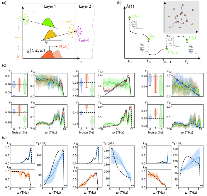
Figure 2: The forward model, optimization process, and performance of the proposed framework on synthetic data. (a) Schematic illustration of the theoretical model. Each phonon mode of frequency $\omega$ propagates its energy (characterized by the distribution $g(t,x,\omega)$) at its group velocity $v(\omega)$ obeying the BTE. At the material boundary of layer 1, only partial energy ($1-\varepsilon_{1}$) gets diffusely back scattered, while the rest dissipates into the environment. At the interface between two layers, the energy from layer 1 is transmitted (reflected) diffusely with coefficients $T_{12}(\omega)$ ($1-T_{12}(\omega)$). (b) Illustration of the adjoint-state method, where the continuous backward trajectories (solid curves with leftward arrows) indicate evolutions induced by $\lambda\frac{\partial h}{\partial\lambda}$ in the Eq. (3), the dashed vertical lines correspond to sudden changes due to the presences of discrete measurement data points and correspond to $\frac{\partial L}{\partial g}$ (the illustration is adapted from Fig. 2 in the Ref. chen_neural_2018). Inset: simultaneous optimization of independently-initialized phonon parameters. (c) Representative reconstructions of $\varepsilon_{1/2}$ and transmittance $T_{12/21}(\omega)$ in the absence of noise (blue) the presence of $\delta=0.05,0.1$ noise (orange and green, respectively) of a $5\,\mathrm{nm}$ Al₂O₃ and $35\,\mathrm{nm}$ Al heterostructure. The Al₂O₃ and Al layers correspond to the subscripts 1 and 2, respectively. (d) Representative reconstructions for transmittance and relaxation times from synthetic MSDs of a $5\,\mathrm{nm}$ Au and $35\,\mathrm{nm}$ Si heterostructure. The Au and Si layers correspond to subscripts 1 and 2, respectively. The solid lines and shaded areas represent the mean reconstructions and those within one standard deviation, respectively. The dashed lines indicate true values. The statistics presented here is obtained from 20 sets of independently initialized initial parameters.

Numerical Verifications

The ground-truth transmittance of a real experimental sample are largely inaccessible by other experimental methods. We first benchmark our framework over numerically simulated MSDs (synthetic data) with known ground truth $\theta^{\mathrm{gt}}$ on a $5\,\mathrm{nm}$ Al₂O₃ and $35\,\mathrm{nm}$ Al heterostructure. As shown in Fig. 2(c), comparisons between $\bar{\theta}^{(\mathrm{f})}$ (solid lines for averages and shaded areas for standard deviations) and $\theta^{\mathrm{gt}}$ (dashed lines) are made for three representative sets of phonon transmittance $T_{12/21}(\omega)$ (right panels) and material-air boundary energy loss coefficients $\varepsilon_{1/2}$ (left panels). Five sets of MSD with distinct initial conditions are used to perform the reconstructions (Supplementary Information Table LABEL:SI_tab:initial_conditions_Al2O3_Al). Excellent agreements are obtained for both reconstructions of the $T_{12/21}(\omega)$ and $\varepsilon_{1/2}$. We notice that the extracted transmittance are spread around $\mathcal{T}^{\mathrm{gt}}$ with larger standard deviations. This behavior can be understood by noting that transmittance only affects a portion of phonon energies in different layers but has no direct influence on the total energy in the heterostructure, while the $\varepsilon$’s directly determine the energy exchange rate with the external environment at material boundaries and dominates the overall trend of $\langle u^{2}(t)\rangle$. The comparatively lower impact of transmittance leads to slower convergence during the learning process compared to that of energy loss coefficients. However, after sufficient number of training epochs, our framework can successfully capture these nuanced properties, as the averaged reconstructions faithfully reflect key features of the true profiles.

To prepare for realistic experimental extraction, we simulate noisy measurements by perturbing the computed MSD according to $\langle u^{2}(t_{n})\rangle_{\mathrm{noisy}}^{\mathrm{target}}=\delta(t_{n})\langle u^{2}(t_{n})\rangle^{\mathrm{target}}$, where the prefactor $\delta(t_{n})$ at each time point $t_{n}$ is randomly drawn from a uniform distribution $\delta(t_{n})\sim\mathcal{U}[1-\delta,1+\delta]$ with $0\leq\delta\leq 1$ representing the noise level. In Fig. 2(c), we demonstrate three representative sets of reconstructions, where different colors (blue, orange, green) represent the reconstructions under different levels of noises ($\delta=0\%,\,5\%,\,10\%$). We see that even with broader spread of the retrieved properties with increased noise level $\delta$ grows, reasonable agreements between reconstructed and ground truth values are still largely maintained. This suggests that our framework is capable of accommodating moderate noises.

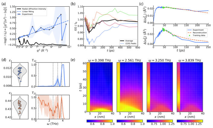
Figure 3: Reconstructions of phonon transport properties from experimentally-measured UED of the Au/Si heterostructure. (a) Representative linear fitting of $-\log(I/I_{0})$ versus $q^{2}$ to extract the MSD from the Au diffraction ring intensities at a particular delay time moment. The $\langle u_{0}^{2}\rangle$ and $I_{0}$ represent room-temperature MSD and diffraction intensity, respectively. This process can be repeated for every collected time point to obtain the complete time-dependent $\langle u_{\mathrm{Au}}^{2}(t)\rangle$. (b) Time-dependent diffraction intensities of Si at $(220)$ and equivalent $\mathbf{q}$-points (transparent thin lines). The MSD of Si is extracted from the averaged intensities (the thick black line). (c) Comparisons between measured and reconstructed MSDs of the Au (top panel) and Si (bottom panel) layers as functions of the delay time. (d) Reconstructed energy loss coefficients and transmittance. The statistics presented here is obtained from 20 sets of independently initialized parameters. (e) Evolution of normalized phonon energy distributions at selected frequencies, $\int_{-1}^{1}g(t,x,\omega,\mu)\ \mathrm{d}\mu/\int_{-1}^{1}g(t_{0},x,\omega,\mu)\ \mathrm{d}\mu$. The frequencies of four panels from left to right correspond to the same order of dashed vertical lines shown in part (d). The Au/Si interface is located at $x=5\,\mathrm{nm}$.

With the success of Al/Al₂O₃ noise test, we further study a 5nm Au/35nm Si heterostructure, which is the same material used in experiments. We can further extend the proposed framework to extract phonon relaxation times. However, we note that the reconstruction of relaxation times is typically more challenging due to short signal time span and even lower gradient magnitudes (Supplementary Information Fig. LABEL:fig:SI_gradients). This indicates that better knowledge about energy loss coefficients and transmittance are desirable to extract relaxation times from experiments. For simplicity, here we assume that the energy loss coefficients of both layers and the relaxation time of the second layer in a heterostructure are known, and perform simultaneous recovery on transmittance $\mathcal{T}(\omega)$ on both layers and relaxation times $\tau(\omega)$ of the first layer. In Fig. 2(d), we show three representative reconstructions of transmittance $\mathcal{T}(\omega)$ and relaxation times $\tau_{\mathrm{Au}}(\omega)$ from synthetic MSDs of the $5\,\mathrm{nm}$ Au/$35\,\mathrm{nm}$ Si heterostructure. More details about reconstructions of $\mathcal{T}(\omega)$ and $\tau(\omega)$ are discussed in Supplementary Information LABEL:SI_subsec:recon_T_tau.

Application to experimental data

We conduct UED measurements on a heterostructure composed of $5\,\mathrm{nm}$ thick polycrystalline Au and $35\,\mathrm{nm}$ thick (001)-oriented single crystal Si membrane fabricated with micro-electromechanical system (MEMS) at MeV-UED beamline at LCLS, SLAC National Accelerator Laboratory. We obtain the time-resolved diffraction patterns consisting of diffraction rings (Au) and Bragg spots (Si) (see a representative example in Supplementary Information Fig. LABEL:fig:SI_schematic_spectrum_diffraction). For each diffraction pattern at a given time delay $t$, the MSDs of each layer can be extracted separately. For the Au layer, we use the full $q$-dependent intensities to perform linear fitting between $-\log(I(t)/I_{0})$ and $q^{2}$ (Fig. 3(a) shows the linear fitting for a particular delay time moment), which can be repeated over all measured time points to obtain $\langle u_{\mathrm{Au}}^{2}(t)\rangle$. While for the Si layer, diffraction spot intensities from the $(220)$ family with high signal-to-noise ratio are used (Fig. 3(b)). We attribute the asymmetric diffraction intensities (shown by the four transparent lines in Fig. 3(b)) observed in the equivalent $\mathbf{q}$-points of Si to a possibly rugged Au/Si interface due to mismatches of in-plane thermal strains at two sides after the pump laser excitation^{harb2009excitation}, which shall not affect the cross-plane transport. The resulting MSDs are plotted as solid lines in Fig. 3(c). More details about experiment data analysis are presented in Supplementary Information LABEL:SI_sec:experiment_method.

The proposed framework can then be applied to learn transmittance from experimental MSDs. In particular, given the existence of plateau in the $\langle u_{\mathrm{Au}}^{2}(t)\rangle$, the initial time $t_{0}$ is chosen to be the moment when $\langle u_{\mathrm{Si}}^{2}(t)\rangle$ reaches maximum, which occurs at $t_{0}\approx 42.8\,\mathrm{ps}$. The initial phonon energy distribution is taken to be at equilibrium, namely $g(t_{0},x,\omega,\mu)=g^{\mathrm{eq}}(t_{0},x,\omega)\equiv\frac{1}{4\pi}\hbar\omega D(\omega)f_{\mathrm{BE}}(T(t_{0},x))$ for each layer, with the initial temperature $T(t_{0},x)$ being uniform in space $x$. The initial temperatures of each layer are solved using Eq. (1) to match $\langle u^{2}(t_{0})\rangle$, resulting in $T_{\mathrm{Au}}\approx 495.6\,\mathrm{K}$ and $T_{\mathrm{Si}}\approx 610.3\,\mathrm{K}$.

The subsequent MSDs collected over the total time of $t_{f}-t_{0}\approx 57\,\mathrm{ps}$, indicated by circular markers in Fig. 3(c), serve as the target $\langle u^{2}\rangle^{\mathrm{target}}$ to obtain the reconstructed transmittance displayed in Fig. 3(d). Due to the lack of “ground truth” parameters of the experiment data, we are unable to directly quantify the reconstruction performance. However, numerical experiments can be performed with synthetic MSDs prepared at exactly the same delay time points, initial temperatures (training samples), and comparable noise level, building a level of confidence (Supplementary Information LABEL:SI_subsec:numexp_AuSi). Due to the limited data points and a single training sample in experimental data, our framework was not able to achieve full reconstruction performance as done in noisy synthetic data shown in Fig. 2. Even so, the reconstruction on transmittance can still shed light on the interfacial thermal transport with a fine frequency-dependent knowledge.

With the phonon transmittance reconstructued in Fig. 3(d), we are then able to reveal the real-time, real-space, and frequency-dependent dynamics of the phonon energy flow in the heterostructure (Fig. 3(e)). Due to the relatively high surface energy loss coefficients of the Si layer ($\bar{\varepsilon}_{\mathrm{Si}}\approx 0.43$), phonon energies decrease rapidly at the boundary $x=40\,\mathrm{nm}$ through boundary scattering. The relative magnitudes of the mode-integrated energy distributions at the interface ($x=5\,\mathrm{nm}$) of both layers indicate a positive energy flux from the Si layer to the Au layer, as dictated by $T_{21}(\omega)$, resulting in a slightly increased lattice temperature of the Au shortly after $t_{0}$. As to the Au layer, the energy distribution $g_{\mathrm{Au}}(t,x,\omega)$ is spread more uniformly, due to its smaller thickness, lower energy loss coefficients ($\bar{\varepsilon}_{\mathrm{Au}}\approx 0.01$) and effect from transmittance $T_{12}(\omega)$. Valuable insight about microscopic phonon transport is gained from the frequency-resolved evolution of the solid angle-integrated, normalized energy distribution, $\int_{-1}^{1}g(t,x,\omega,\mu)\ \mathrm{d}\mu/\int_{-1}^{1}g(t_{0},x,\omega,\mu)\ \mathrm{d}\mu$, shown in Fig. 3(e), where we observe that the evolution of energy distributions of different phonon mode vary significantly, especially at the Au/Si interface. These and other quantitative analyses are made possible by solving the BTE using the reconstructed parameters, which can provide key insights for engineering phonon transport in diverse materials systems.

Discussion and Conclusion

This framework offers a new avenue that can efficiently and comprehensively characterize layer-specific and frequency-resolved thermal transport properties with two key features. One is the additional reciprocal space information, where different layers result in different diffraction spots. This leads to a higher-dimensional input in $(\mathbf{q},t)$ space and enables a simultaneous reconstruction of phonon properties with less sensitivity against noise. The other feature is the capability to capture real phonon dynamics. The initial time can be chosen well after the pulse excitation and full thermalization of hot electrons without hampering information extraction, and the analysis of Debye-Waller factor focuses on the atomic displacements with minimal interference of the electronic degrees of freedom.

There are still a few improvements and generalization can be done based on this framework. First, the validation of the extracted parameters from experimental is challenging. The partial information agreement with experimental measurements and the high-quality benchmark with computational data build a level of confidence, yet additional independent experimental validation will build further confidence on the extracted information, such as parameters like $T_{12}(\omega)$. Second, we have assumed that there is no coupling between phonons with different frequencies or inelastic scattering. This allows us to treat each phonon frequency channel independently but limits its application in the strongly anharmonic regime. Future incorporation on anharmonic effects are feasible with further modification of the framework. Third, we have assumed that the phonon DOS $D(\omega)$ and group velocities $v(\omega)$ are known, yet in nanostructures, they may be subject to change due to size effect. We note that the drastic size effect is only apparent for very thin, few-nm-thick films ^Balandin2005, and even in that regime, $D(\omega)$ and $v(\omega)$ are still computable with relatively high fidelity. The effect of $D(\omega)$ and $v(\omega)$ are subject to further investigation.

In this work, we develop a machine learning-informed computational framework to analyze the time-resolved diffraction patterns in UED to infer frequency-resolved interfacial thermal transport at the nanoscale. The same principle is also applicable to other time-resolved diffraction experiments. The combination of the adjoint-state and automatic differentiation machine learning approach makes the BTE model differentiable with respect to its phonon properties without compromising physical validity. We demonstrate its power in reliably learning multiple phonon properties in distinct scenarios, as well as its robustness against measurement noise. Our approach opens up a new way to study frequency-resolved nanoscale thermal transport with foreseeable impact in the areas of improving thermal management to realize higher energy efficiency, facilitate sustainable usage of natural resources, and reduce global warming. Given the generality of automatic differentiation and the adjoint-state method for solving differential-equation based physical models, we anticipate the framework could benefit the study of a wide range of physical systems, enabling the acquisition of hidden information from complex observables in a dynamical system and informing the design of better measurement strategies.

Methods

Forward solving and backward parameter extraction for BTE

To establish the forward model to solve the BTE, we need boundary conditions, initial conditions and detailed balance conditions. The mismatch of vibrational properties at the interface allows only partial transmission of the phonon energy across the interface while the rest is reflected. Therefore, the energy flux $\mathcal{F}^{\pm}(t,x,\omega)=\int_{\mu\gtrless 0}\mu v(\omega)g(t,x,\omega,\mu)\ \mathrm{d}\mu$ at the interface $x=x_{\mathrm{intf}}$ can be described by the interfacial boundary condition

$$\begin{split}\mathcal{F}_{2}^{+}(t,\omega)&=T_{12}(\omega)\mathcal{F}_{1}^{+}(t,\omega)+[1-T_{21}(\omega)]\mathcal{F}_{2}^{-}(t,\omega),\\ \mathcal{F}_{1}^{-}(t,\omega)&=[1-T_{12}(\omega)]\mathcal{F}_{1}^{+}(t,\omega)+T_{21}(\omega)\mathcal{F}_{2}^{-}(t,\omega),\end{split}$$ (4)

where the subscripts $1,\,2$ denote the two sub-layers in the heterostructure; for instance $T_{12}(\omega)$ is the transmittance from layer 1 to 2. Since we only analyze $q$-dependent diffraction signals, the wavevector dependencies are not taken into account and mode conversion among different phonon polarizations is neglected for simplicity. Meanwhile, we restrict our attention to elastic phonon scatterings, the two sets of transmittance $T_{12}(\omega)$ and $T_{21}(\omega)$ are connected by the detailed balance ^{swartz1989thermal}, $T_{12}(\omega)v_{1}(\omega)D_{1}(\omega)=T_{21}(\omega)v_{2}(\omega)D_{2}(\omega)$. Meanwhile, phonons are assumed to be diffusely backscattered at material-air boundaries with energy loss parameterized by $\varepsilon_{1}$ and $\varepsilon_{2}$, respectively^hua2015semi. We note that the $\varepsilon_{1}$ and $\varepsilon_{2}$ here only serve as phenomenological descriptions of the energy exchanging rate between the phonon system and the external environment. In addition to interface and boundary conditions, We choose initial condition $g(t_{0},x,\omega)=\frac{1}{4\pi}\hbar\omega D(\omega)(f_{\mathrm{BE}}(T)-f_{\mathrm{BE}}(T_{0}))$ at $t=t_{0}$, a moment after full thermalization of hot electrons. This is feasible since in an UED setup we can simply choose a $t_{0}$ after the maximum $\langle u^{2}\rangle$ is reached. In addition, the initial temperature profile is assumed to be spatially uniform with $T(t_{0},x)\equiv T(t_{0})$. A more detailed formulation is presented in Supplementary Information LABEL:SI_sec:boltzmann_transport_equations.

In the backward loop, one advantage of using the adjoin-state method is that there is large freedom to choose which parameters as known and which parameters are unknown and to be extracted. Since the phonon DOS $D(\omega)$ and group velocities $v(\omega)$ can be reliably computed from ab initio methods^{minnich2015advances}, they are considered as known. Our discussions thus focus on reconstructing other phonon transport properties that are more challenging to obtain by conventional methods, such as frequency-dependent transmittance. Though phonon branch dependencies can be taken into account by our formalism, we restrict our attention to branches-averaged phonon transport in this work. In particular, we make use of the weighted average group velocities and relaxation times with DOS of each branch, for example, $v(\omega)=\sum_{r}D_{r}(\omega)v_{r}(\omega)/\sum_{r}D_{r}(\omega)$. The detailed-balance constraint between $T_{12}(\omega)$ and $T_{21}(\omega)$ allows us to choose the training parameters $\mathcal{T}(\omega_{n})=\max(T_{12}(\omega_{n}),T_{21}(\omega_{n}))$ at each frequency $\omega_{n}$. The $\varepsilon\in[0,1]$ could vary between samples and is also considered as unknown. Provided the minimum amount of prior knowledge, the fitting parameters $\theta$ is randomly initialized (Supplementary Information LABEL:SI_subsec:init_params). Given the high dimensionality of fitting parameters $\theta$, the loss landscape could be extremely complex and non-convex, which typically results in $\theta^{(0)}$-dependent final predictions $\theta^{(\mathrm{f})}$. To address this issue, we simultaneously optimize a set of independently-initialized parameters $\{\theta_{1}^{(0)},\theta_{2}^{(0)}\ldots,\theta_{N}^{(0)}\}$, and the final predictions are obtained by averaging over the ensemble, for example, $\bar{\theta}^{(\mathrm{f})}=\frac{1}{N}\sum_{n=1}^{N}\theta_{n}^{(\mathrm{f})}$. The benefit of this approach can be intuitively understood as approaching the ground truth $\theta^{\mathrm{gt}}$ with a population $\{\theta_{n}^{(\mathrm{f})}\}$ from different directions, schematically illustrated in Fig. 2(b). While each cluster may be trapped in a local minimum around $\theta^{\mathrm{gt}}$, the averaged $\bar{\theta}^{(\mathrm{f})}$ can generally cancel the influence of individual local minima and thus provide a better estimate.