Fairness-aware Configuration of Machine Learning Libraries

Abstract.

This paper investigates the parameter space of machine learning (ML) algorithms in aggravating or mitigating fairness bugs. Data-driven software is increasingly applied in social-critical applications where ensuring fairness is of paramount importance. The existing approaches focus on addressing fairness bugs by either modifying the input dataset or modifying the learning algorithms. On the other hand, the selection of hyperparameters, which provide finer controls of ML algorithms, may enable a less intrusive approach to influence the fairness. Can hyperparameters amplify or suppress discrimination present in the input dataset? How can we help programmers in detecting, understanding, and exploiting the role of hyperparameters to improve the fairness?

We design three search-based software testing algorithms to uncover the precision-fairness frontier of the hyperparameter space. We complement these algorithms with statistical debugging to explain the role of these parameters in improving fairness. We implement the proposed approaches in the tool Parfait-ML (PARameter FAIrness Testing for ML Libraries) and show its effectiveness and utility over five mature ML algorithms as used in six social-critical applications. In these applications, our approach successfully identified hyperparameters that significantly improve (vis-a-vis the state-of-the-art techniques) the fairness without sacrificing precision. Surprisingly, for some algorithms (e.g., random forest), our approach showed that certain configuration of hyperparameters (e.g., restricting the search space of attributes) can amplify biases across applications. Upon further investigation, we found intuitive explanations of these phenomena, and the results corroborate similar observations from the literature.

1. Introduction

Data-driven software applications are an integral part of modern life impacting every aspect of societal structure, ranging from education and health care to criminal justice and finance (Northpointe, 2012; Deloitte, 2021). Since these algorithms learn from prior experiences, it is not surprising that they encode historical and present biases due to displacement, exclusion, segregation, and injustice. The resulting software may particularly disadvantage minorities and protected groups and be found non-compliant with law such as the US Civil Rights Act (Blumrosen, 1978). Therefore, helping programmers detect and mitigate fairness bugs in social-critical data-driven software systems is crucial to ensure inclusion in our modern, increasingly digital society.

The software engineering (SE) community has invested substantial efforts to improve the fairness of ML software (Galhotra et al., 2017; Aggarwal et al., 2019; Udeshi et al., 2018; Zhang et al., 2020b; Chakraborty et al., 2020). Fairness has been treated as a critical meta-properties that requires an analysis beyond functional correctness and measurements such as prediction accuracy (Brun and Meliou, 2018). However, the majority of previous work within the SE community evaluates fairness on the ML models after training (Galhotra et al., 2017; Udeshi et al., 2018; Aggarwal et al., 2019; Zhang et al., 2020b), while the programmer supports to improve fairness during the inference of models (i.e., training process) is largely lacking.

The role of training processes in amplifying or suppressing vulnerabilities and bugs in the input dataset is well-documented (Zhang et al., 2020a). The training process typically involves tuning of hyperparameters: variables that characterize the hypothesis space of ML models and define a trade-off between complexity and performance. Some prominent examples of hyperparameters include l1 vs. l2 loss function in support vector machines, the maximum depth of a decision tree, and the number of layers/neurons in deep neural networks. Hyperparameters are crucially different from the ML model parameters in that they cannot be learned from the input dataset alone. In this paper, we investigate the impact of hyperparameters on ML fairness and propose a programmer support system to develop fair data-driven software.

We pose the following research questions: To what extent can hyperparameters influence the biases present in the input dataset? Can we assist ML library developers in identifying and explaining fairness bugs in the hyperparameter space? Can we help ML users to exploit the hyperparamters to imporive fairness?

We present Parfait-ML (PARameter FAIrness Testing for ML Libraries): a search-based testing and statistical debugging framework that supports ML library developers and users to detect, understand, and exploit configurations of hyperparameters to improve ML fairness without impacting functionality. We design and implement three dynamic search algorithms (independently random, black-box evolutionary, and gray-box evolutionary) to find configurations that simultaneously maximize and minimize group-based fairness with a constraint on the prediction accuracy. Then, we leverage statistical learning methods (Kampmann et al., 2020; Tizpaz-Niari et al., 2018) to explain what hyperparameters distinguish low-bias models from high-bias ones. Such explanatory models specifically aid ML library maintainers to localize a fairness bug. Finally, we show that Parfait-ML can effectively (vis-a-vis the state-of-the-art techniques) aid ML users to find a configuration that mitigates bias without degrading the prediction accuracy.

We evaluate our approach on five well-established machine learning algorithms over six fairness-sensitive training tasks. Our results show that for some algorithms, there are hyperparameters that consistently impact fairness across different training tasks. For example, max_feature parameter in random forest can aggravate the biases for some of its values such as $\log_{2}$(#num. features) beyond a specific training task. These observations corroborate similar empirical observations made in the literature (Zhang and Harman, 2021).

In summary, the key contributions of this paper are:

1. the first approach to support ML library maintainers to understand the fairness implications of algorithmic configurations;

2. three search-based algorithms to approximate the Pareto curve of hyperparameters against the fairness and accuracy;

3. a statistical debugging approach to localize parameters that systematically influence fairness in five popular and well-establish ML algorithms over six fairness-critical datasets;

4. a mitigation approach to effectively find configurations that reduce the biases (vis-a-vis the state-of-the-art); and

5. an implementation of Parfait-ML (PARameter FAIrness Testing for ML Libraries) and its experimental evaluation on multiple applications, available at: https://github.com/Tizpaz/Parfait-ML.

2. Background

Fairness Terminology and Measures. Let us first recall some fairness vocabulary. We consider binary classification tasks where a class label is favorable if it gives a benefit to an individual such as low credit risk for loan applications (default), low reoffend risk for parole assessments (recidivism), and high qualification score for job hiring. Each dataset consists of a number of attributes (such as income, employment status, previous arrests, sex, and race) and a set of instances that describe the value of attributes for each individual. We assume that each attribute is labeled as protected or non-protected. According to ethical and legal requirements, ML software should not discriminate on the basis of an individual’s protected attributes such as sex, race, age, disability, colour, creed, national origin, religion, genetic information, marital status, and sexual orientation.

There are several well-motivated characterizations of fairness. Fairness through unawareness (FTU) (Dwork et al., 2012) requires masking protected attributes during training. However, $FTU$ is not effective since protected and non-protected attributes often correlate (e.g., ZIP code and race), and biases are introduced from non-protected attributes. Fairness through awareness (FTA) (Dwork et al., 2012) is an individual fairness notion that requires that two individuals with similar non-protected attributes are treated equally.

Group fairness requires the statistics of ML outcomes for different protected groups to be similar (Hardt et al., 2016). There are multiple metrics to measure group fairness in ML software. Among them, equal opportunity difference (EOD) measures the difference between the true positive rates (TPR) of two protected groups. Similarly, average odd difference (AOD) is the average of differences between the true positive rates (TPR) and the false positive rates (FPR) of two protected groups (Bellamy et al., 2019; Chakraborty et al., 2020; Zhang and Harman, 2021). These metrics can naturally be generalized to handle situations where protected attributes may have more than two values. For instance, if race is a protected attribute, then the EOD is the maximum EOD among any two race groups. This paper focuses on group fairness.

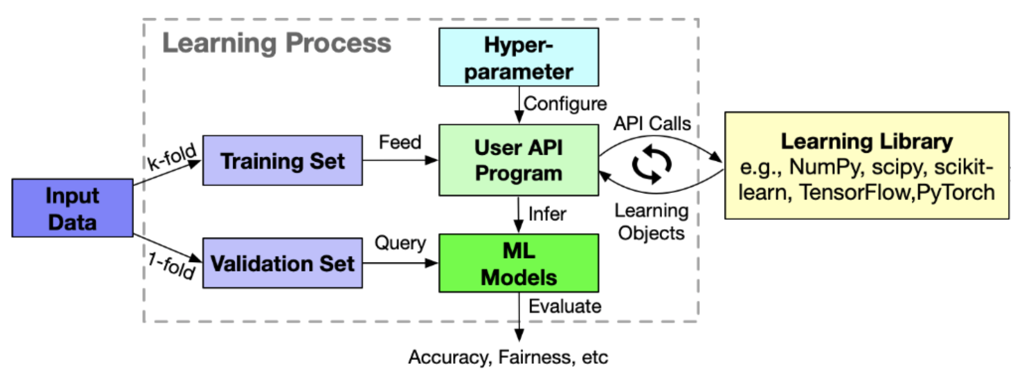
Figure 1. Data-Driven Software System Developments

Data-Driven Software Systems. Data-driven software is distinguished from common software in that they largely learn their decision logic from datasets. Consequently, while the traditional software developers explicitly encode decision logic via control and data structures, the ML programmers and users provide input data, perform some pre-processing, choose ML algorithms, and tune hyperparameters to enable data-driven systems to infer a model that encodes the decision logic.

Figure 1 shows the key components of a data-driven system. At a high-level, a data-driven system consists of three major components: input data, a learning (training) process, and a library framework. The ML users often provide input data and build an ML model using a programming interface. The interface interacts with the core ML library (e.g., scikit-learn, TensorFlow, etc) and constructs different instances of learning algorithms using hyperparameters. Then, they feed the training data into the constructed learning objects to infer the parameters of an ML model.

As a part of the training process, ML users query the ML model with the validation set to evaluate functional metrics such as prediction accuracy and non-functional metrics such as EOD for group fairness. At the heart of the learning process, tuning hyperparameters is particularly challenging since they cannot be estimated from the input data, and there is no analytical formula to calculate an appropriate value (Kuhn et al., 2013). We distinguish algorithm parameters (i.e., hyperparameters) such as tolerance of optimization in SVMs, maximum features to search in random forest, and minimum samples in leaf nodes of decision trees that set before training from model parameters that are inferred automatically after training such as the split feature of decision tree nodes, the weights of neurons in neural networks, and coefficients of support vector machines.

Related Work. 1) Evaluating fairness of ML models. Themis (Galhotra et al., 2017) presents a causal testing approach to measure group discrimination on the basis of protected attributes. Particularly, they measure the difference between the fairness metric of two subgroups by counterfactual queries; i.e., they sample inputs where the protected attributes are A and compare the fairness to a counterfactual scenario where the protected attributes are set to B. Agarwal et al. (Aggarwal et al., 2019) present a black-box testing technique to detect individual discrimination: two people with similar features other than protected ones receive different ML predictions. They approximate ML models with decision trees and use symbolic execution techniques over the tree structure to find discriminatory instances. Udeshi et al. (Udeshi et al., 2018) present a two-step technique that first uniformly and randomly search the input data space to find a discriminatory instance and then locally perturb those instances to further generate biased test cases. Adversarial discrimination finder (Zhang et al., 2020b) is an adversarial training method to generate individual discrimination instances in deep neural networks. These works focus on testing individual ML models and improving their fairness. We focus on ML libraries and study how algorithm configurations impact fairness.

2) Inprocessing methods for bias reduction. A body of work considers inprocess algorithms to mitigate biases in ML predictions. Adversarial debiasing (Zhang et al., 2018) is a technique based on adversarial learning to infer a classifier that maximizes the prediction accuracy and simultaneously minimizes adversaries’ capabilities to guess the protected attribute from the ML predictions. Prejudice remover (Kamiran et al., 2012) adds a fairness-aware regularization term to the learning objective and minimizes the accuracy and fairness loss. This line of work requires the modification of learning algorithms either in the loss function or the parameter of ML models. Exponentiated gradient (Agarwal et al., 2018) is a meta-learning algorithm to mitigate biases. The approach infers a family of classifiers to maximize prediction accuracy subject to fairness constraints. Since this approach assumes black-box access to the learning algorithms, we evaluate the effectiveness of Parfait-ML in mitigating biases with this baseline (see Subsection 6.7).

3) Combining pre-processing and inprocessing bias reductions. Fairway (Chakraborty et al., 2020) uses a two step mitigation approach. While pre-processing, the dataset is divided into privileged and unprivileged groups where the respective ML models train independently from one another. Then, they compare the prediction outcomes for the same instance to find and remove discriminatory samples. Given the pre-processed dataset, the inprocess step uses a multi-objective optimization (FLASH) (Nair et al., 2020) to find an algorithm configuration that maximizes both accuracy and fairness. The work focuses on using hyperparameters to mitigate biases in a subset of hyperparameters and a limited number of algorithms. In particular, they require a careful selection of relevant hyperparameters. Our approach, however, does not require a manual selection of hyperparameters. Instead, our experiments show that the evolutionary search is effective in identifying and exploiting fairness-relevant hyperparameters automatically. In addition, our approach explains what hyperparameters influence fairness. Such explanatory models can also pinpoint whether some configurations systematically influence fairness, which can be useful for Fairway to carefully select a subset of hyperparameters in its search. To show the effectiveness of Parfait-ML in reducing biases, we compare our approach to Fairway (Chakraborty et al., 2020, 2019) (see Subsection 6.7).

3. Overview

We use the example of random forest ensemble (scikit learn, 2021d) to overview how Parfait-ML assists ML developers and users to discover, explain, and mitigate fairness bugs by tuning the hyperparameters.

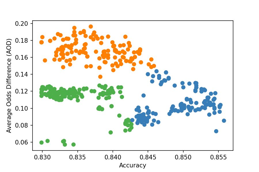
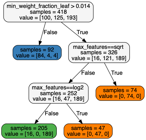
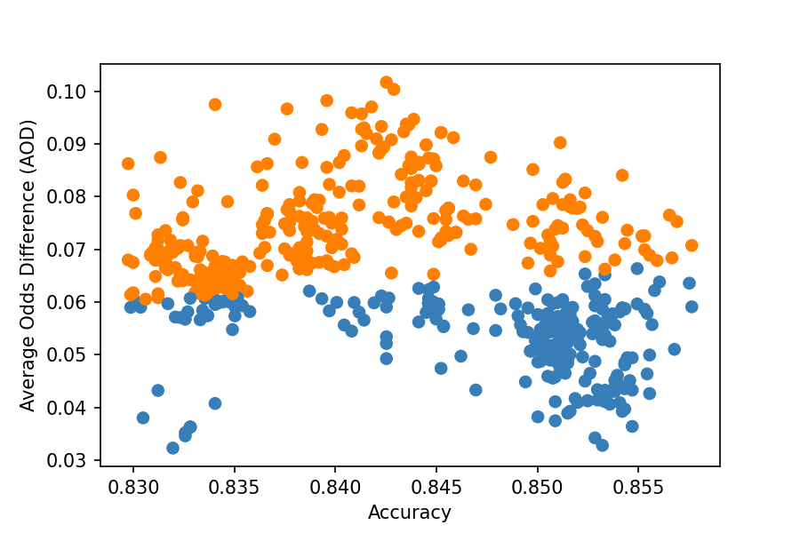
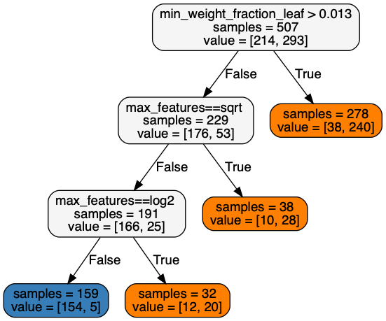
Figure 2. (a) Test cases for $census$ with $sex$ are clustered into three: y-axis is the $AOD$ bias and x-axis is the accuracy; (b) The tree classifier explains that the max_features and the min_weight_fraction_leaf discriminate the three clusters; (c) Two clusters for $census$ with $race$; (d) The classifier for $census$ with $race$ shows a similar explanation to $census$ with $sex$.

Dataset. Adult Census Income (Dua and Graff, 2017a) is a binary classification dataset that predicts whether an individual has an income over $50K$ a year. The dataset has $48,842$ instances and $14$ attributes. For this overview, we start by considering sex as the protected attribute.

Learning Algorithm. Random forest ensemble is a meta estimator that fits a number of decision trees and uses the averaged outcomes of trees to predict labels. The ensemble method includes $18$ parameters. Three parameters are boolean, two are categorical, six are integer, and seven are real variables. Examples of these parameters are the maximum depth of the tree, the number of estimator trees, and the minimum impurity to split a node further.

Fairness and Accuracy Criterion. We randomly divide the dataset into $4$-folds and use $75\%$ of the dataset as the training set and $25$% as the validation set. We measure both accuracy and fairness metrics after training on ML models using the validation set. We report the average odd difference ($AOD$) as well as the equal opportunity difference ($EOD$), which were introduced in Background Section 2. Our accuracy metric is standard: the fraction of correct predictions.

Test Cases. Our approach has three options for generating test cases: independently random, black-box mutations, and gray-box mutations. In this section, we use the black-box mutations (see RQ2 in Section 6.5). We run the experiment $10$ times, each for $4$ hours (the default number of repetition and time-out). We obtain an average of $603$ valid test cases over $10$ runs. Since the default parameters of random forests achieve an accuracy of $84\%$, a valid test case achieves similar or better accuracy. To allow finding a fair configuration in cases where the default configurations are the most accurate model, we tolerate $1\%$ accuracy degradations. The overall accuracy of ML models over the entire corpus of test cases varies from $83\%$ to $85.7\%$. Each test case includes the valuation of $18$ algorithm parameters, accuracy, $AOD$, and $EOD$.

Magnitude of Biases. We report the magnitude of group biases in the hyperparameter space of random forests. The minimum and maximum $AOD$ are $5.8\%(+/-0.6\%)$ and $19.0\%(+/-0.4\%)$, respectively. The values are the average of $10$ runs, with $95\%$ confidence interval reported in the parenthesis, and higher values indicate stronger biases. Similarly, the minimum and maximum $EOD$ are $4.8\%(+/-0.4)$ and $32.3\%(+/-0.6)$. These results show that within $2.7\%$ accuracy margins, there can be over $13\%$ and $27\%$ difference in $AOD$ and $EOD$, respectively. These results indicate that different configurations of random forests can indeed amplify or suppress the biases from the input dataset. The details of relevant experiments for different datasets and learning algorithms are reported in RQ1 (Section 6.4).

Explanation of Biases. Our next goal is to explain what configurations of hyperparameters influence group-based fairness.

Clustering. We first partition generated test cases in the domain of fairness ($AOD$) versus accuracy. Particularly, we apply the Spectral clustering algorithm where the number of partitions are set to three. Figure 2 (a) shows the three clusters identified from the generated test cases. Looking into the figure, we see that green and orange clusters have similar accuracy; however, they have significantly different biases ($AOD$). Additionally, the blue cluster achieves better accuracy with a similar $AOD$ to the green cluster.

Tree Classifiers. Next, we use CART tree classifiers (Breiman et al., 1984) to explain the differences between the clusters in terms of algorithm parameters as shown in Figure 2 (b). Each node in the tree shows a split parameter, the number of samples reaching the node, and sample distributions in different clusters. First, let us understand the differences between the green and orange clusters. The decision tree shows that the max_feature parameter distinguishes these two clusters. While the values ‘auto’ and ‘None’ do not restrict the number of features during training, ‘sqrt’ and ‘log2’ randomly choose a subset of features according to the square root and the base-2 logarithm of total features during training. This explanation validates findings from Zhang and Harman (Zhang and Harman, 2021) where they reported that restricting the number of features strengthens the biases in ML models. Another localized parameter is the minimum sample to stop the growth and fit leaf models. This distinguishes the orange cluster from the two other clusters. Intuitively, underprivileged groups tend to have less representation in the dataset. Since random forests assign predictions to the majority class in the leaves, they tend to favor privileged groups when a threshold on the minimum samples is set.

Feature Transferability. In another experiment, we consider the $race$ attribute as the protected using the $census$ dataset. Figure 2 (c) shows the inputs generated for the race feature is clustered into two groups. The explanation tree in Figure 2 (d) shows that the max feature and minimum samples in leafs are two parameters in the tree regressor that explain the difference in the $AOD$ biases, similar to the case when $sex$ is the protected attribute.

Dataset Transferability. We also study other datasets in ML fairness literature including the German Credit Data (Credit) (Dua and Graff, 2017b) (see Section 6.6). For the random forest, our findings are stable across different datasets and protected attributes: the minimum sample weights of leaf nodes and maximum features are the most important parameters to distinguish configurations with high and low biases. These results can help ML developers understand the fairness implications of different configuration options in their libraries.

Mitigation Technique. As we discussed previously, Parfait-ML is also useful to suppress biases by picking low-bias hyperparameters. The details of experiments to show the mitigation aspect of Parfait-ML can be found in Section 6.7. For random forests, Parfait-ML can mitigate the biases from an $EOD$ of $11.6\%$ to $0.1\%$ with even better accuracy compared to the default configuration as a baseline. There are cases that Parfait-ML alone cannot reduce biases in a statistically significant way. In such cases, we found that combing Parfait-ML with existing approaches can significantly reduce biases under certain conditions (see RQ4 in Section 6.7).

4. Problem Definition

The primary performance criteria for data-driven software is accuracy. However, the presence of fairness results in a multi-objective optimization problem. We propose a search-based solution to approximate the curve of Pareto-dominant hyperparameter configurations and a statistical learning method to succinctly explain what hyperparameter distinguish high fairness from low fairness.

The ML Paradigm. Data-driven software systems often deploy mature, off-the-shelf ML libraries to learn various models from data. We can abstractly view a learning problem as the problem of identifying a mapping $M:\mathcal{X}\to\mathcal{Y}$ from a set $\mathcal{X}$ of inputs to a set $\mathcal{Y}$ of outputs by learning from a fixed dataset $\mathcal{D}=\left\{({\bf x_{i}},{\bf y_{i}})\right\}_{i=1}^{N}$ so that $M$ generalizes well to previously unseen situations.

The application interfaces of these ML libraries expose configuration parameters—characterizing the set $\mathcal{H}$ of hyperparameters—that let the users define the hypothesis class for the learning tasks. These hypothesis classes themselves are defined over a set of model parameters $\Theta_{h}$ based on the selected hyperparameter $h\in\mathcal{H}$. The ML programs sift through the given dataset $\mathcal{D}$ to learn an “optimal” value $\theta\in\Theta_{h}$ and thus compute the learning model $M_{h}(\theta|\mathcal{D}):\mathcal{X}\to\mathcal{Y}$ automatically. When $\mathcal{D}$ and $\theta$ are clear from the context, we write $M_{h}$ for the resulting model.

The fitness of a hyperparameter $h\in\mathcal{H}$ is evaluated by computing the accuracy (ratio of correct results) of the model $M_{h}$ on a validation dataset $\mathcal{D}_{*}$. We denote the accuracy of a model $M$ over $\mathcal{D}_{*}$ as $ACC^{M}$. The dataset $\mathcal{D}_{*}$ is typically distinct from $\mathcal{D}$ but assumed to be sampled from the same distribution. Hence, the key design challenge for the data-driven software engineering is a search problem for optimal configuration of the hyperparameters maximizing the accuracy over $\mathcal{D}_{*}$.

Fairness Notion. To pose fairness requirements over the learning algorithms, we assume the access to two predicates. The predicate $\pi:\mathcal{X}\to\left\{0,1\right\}$ over the input variables characterizing the protected status of a data point ${\bf x}$ (e.g., race, sex, or age). Without loss of generality, we assume there are only two protected groups: a group with $\pi({\bf x})=0$ and a group with $\pi({\bf x})=1$. We also assume that the predicate $\phi:\mathcal{Y}\to\left\{0,1\right\}$ over the output variables characterizes a favorable outcome (e.g., low reoffend risk) with $\phi({{\bf y}})=1$.

Given $\mathcal{D}_{*}$ and $M:\mathcal{X}\to\mathcal{Y}$, we define true-positive rate (TPR) and false-positive rate (FPR) for the protect group $i\in\left\{0,1\right\}$ as

$$TPR^{M}(i) = \frac{\big{|}\left\{({\bf x},{\bf y})\in\mathcal{D}_{*}:\pi({\bf x})=i,\phi(M({\bf x}))=1,\phi({\bf y})=1\right\}\big{|}}{\big{|}\left\{({\bf x},{\bf y})\in\mathcal{D}_{*}:\pi({\bf x})=i\right\}\big{|}}$$

$$FPR^{M}(i) = \frac{\big{|}\left\{({\bf x},{\bf y})\in\mathcal{D}_{*}:\pi({\bf x})=i,\phi(M({\bf x}))=1,\phi({\bf y})=0\right\}\big{|}}{\big{|}\left\{({\bf x},{\bf y})\in\mathcal{D}_{*}:\pi({\bf x})=i\right\}\big{|}}.$$

We use two prevalent notions of fairness (Bellamy et al., 2019; Chakraborty et al., 2020; Zhang and Harman, 2021). Equal opportunity difference (EOD) of $M$ against $\mathcal{D}_{*}$ between two groups is

$$EOD^{M}=\big{|}TPR^{M}(0)-TPR^{M}(1)\big{|},$$

and average odd difference (AOD) is

$$AOD^{M}=\frac{|TPR^{M}(0)-TPR^{M}(1)|+|FPR^{M}(0)-FPR^{M}(1)|}{2}.$$

Let $\mathcal{F}\in\left\{EOD^{M},AOD^{M}\right\}$ be some fixed fairness criterion. We notice that a high value of $\mathcal{F}$ implies high bias (low fairness) and a low value implies low bias (high fairness).

The key design challenge for social-critical data-driven software systems is to search for fairness- (bias-) optimal configuration $h\in\mathcal{H}$ of hyperparameters maximizing the accuracy and minimizing the bias $\mathcal{F}$ of the resulting model $M_{h}$. A hyperparameter $h\in\mathcal{H}$ is Pareto-fairness-dominated by $g\in\mathcal{H}$ if the model $M_{g}$ provides better accuracy and lower bias, i.e. $ACC^{M_{h}}<ACC^{M_{g}}$ and $\mathcal{F}^{M_{h}}>\mathcal{F}^{M_{g}}$. We say that a hyperparameter $h\in\mathcal{H}$ is Pareto-fairness-optimal if it is not fairness-dominated by any other hyperparameters. Similarly, we can define Pareto-bias-domination ($h$ is Pareto-bias-dominated by $g$ if $ACC^{M_{h}}<ACC^{M_{g}}$ and $\mathcal{F}^{M_{h}}<\mathcal{F}^{M_{g}}$) and Pareto-bias-optimal hyperparamters. A Pareto set is a graphical depiction of all of Pareto-optimal points. Since we are interested in hyperparameters that lead to either low bias (high fairness) or high bias (low fairness), our goal is to compute Pareto sets for both fairness and bias optimal hyperparameters: we call this set a twined Pareto set. Our goal is to compute a convenient approximation of the twined Pareto set that can be used to identify, explain, and exploit the hyperparameter space to improve fairness.

Definition 4.0 (hyperparameter Discovery and Debugging).

5. Approach

We propose dynamic search algorithms to discover hyperparameters that characterize fairness-optimal and bias-optimal models and statistical debugging to localize what hyperparameters distinguish fair models from biased ones.

Input: algorithm $\mathcal{A}$, space of hyperparamters $\mathcal{H}$, default configuration $h_{d}$, training dataset ($X_{T},y_{T}$), test dataset ($X_{t},y_{t}$), protected attribute $A$, type of search $S_{t}$, the margin $\epsilon$, time-out $T$, num. clusters $k$.

Output: Test Cases $I$, Predicates $\Phi$.

1

2$model$, $path$ $\leftarrow$ run($\mathcal{A}$, $h_{d}$, $X_{T}$, $y_{T}$, $S_{t}$)

3$pred$ $\leftarrow$ infer($model$, $X_{t}$)

4$accuracy_{d}$, $fairness_{d}$ $\leftarrow$ metric($pred$, $y_{t}$, $A$)

5$I$.add($h_{d}$, $accuracy_{d}$, $fairness_{d}$, $path$)

6$cur$ $\leftarrow$ time()

7while time() - $cur$ $<$ $T$ do

8      

9      if $S_{t}$ $==$ “random” then

10             $h$ $\leftarrow$ UniformlyRandom($\mathcal{H}$)

11      else if $S_{t}$ $==$ “black-box” or $S_{t}$ $==$ “gray-box”  then

12             $h^{\prime}$ $\leftarrow$ choice_W($I$.project($\mathcal{H}$))

13            $h$ $\leftarrow$ mutate($h^{\prime}$)

14      

15      $model$, $path$ $\leftarrow$ run($\mathcal{A}$, $h$, $X_{T}$, $y_{T}$, $S_{t}$)

16      $pred$ $\leftarrow$ infer($model$, $X_{t}$)

17      $accuracy,fairness$ $\leftarrow$ metric($pred$, $y_{t}$, $A$)

18      if promising($h$, $accuracy$, $\epsilon$, $fairness$, $path$, $I$) then

19             $I$.add($h$, $accuracy$, $fairness$, $path$)

20      

21

22$label$ $\leftarrow$ spectralClust($I.$project($accuracy$, $fairness$), $k$)

23$\Phi$ $\leftarrow$ DTClassifier($I.$project($\mathcal{H}$), $label$)

Algorithm 1 Parfait-ML: Detecting and Explaining Fairness and Bias in parameters of ML algorithms.

Hyperparameter Discovery Problem. The grid search is an exhaustive method to approximate the Pareto curve, however, it suffers from the curse of dimensionality. Randomized search may alleviate this curse to some extent, however, given its blind nature and the large space of parameters, it may fail to explore interesting regions. Evolutionary algorithms (EA) guided by the promising input seeds often explore extreme regions of the Pareto space and are thus natural candidates for our search problem. While multi-objective EAs look promising, they are notoriously slow (Nair et al., 2020). For example, NSGA-II (Deb et al., 2002) has quadratic complexity to pick the next best candidate form the samples in the population. Instead, we propose a single objective EA with accuracy constraints. Algorithm 1 sketches our approach for detecting and explaining strengths of discriminations in the configuration space of ML libraries.

General Search Algorithms. The random search algorithm generates test inputs uniformly and independently from the domain of parameter variables. The black-box search is an evolutionary algorithm that selects and mutates inputs from its population. The gray-box evolutionary search uses the same strategy as the black-box search, but is also guided by the code coverage of libraries’ internals.

Initial Seeds. Our approach starts with the default configuration and runs the learning algorithm over the training dataset to build a machine learning model (line 1 of Algorithm 1). If the search algorithm is gray-box, the running of algorithm also returns the path characterizations. A path characterization is xor of hash values obtained from program line numbers visited in the run. Then, we use the machine learning model and the validation set to infer the predictions (line 2). We use the predictions, their ground-truths, and protected attributes to measure the prediction accuracy and the group fairness metrics such as $EOD$ and $AOD$ (line 3).

Input Selections. We add the default configuration and its outcome to the population (line 4) and iteratively search to find configurations that minimize and maximize biases given a threshold on the accuracy. In doing so, we consider the type of search to generate inputs. If the search is “random”, we randomly and uniformly sample from the domain of configuration parameters (lines 7 to 8). Otherwise, we pick an input from the population based on a weighted sampling strategy that prefers more recent inputs: given a location $i>0$, the probabilistic weight of sample $i$ is $\frac{2*i}{n*(n+1)}$ where $n$ is the size of input population, assuming a higher location is more recent. Then, we randomly choose a parameter and apply mutation operations over its current value to generate a new configuration (lines 9 to 11). We use standard mutation operations such as increasing/decreasing value by a unit. Given the new configuration, we perform the training and inference steps to measure the prediction accuracy and biases (lines 12 to 14).

Search Objective. Identifying promising configurations is a critical step in our algorithm. We consider the characteristics of the new configuration and compare them to the test corpus (line 15). We say a configuration is promising if no existing configuration in the test corpus Pareto-fairness-dominate or Pareto-bias-dominate (based on $EOD$ and $AOD$) the new configuration. Thus, we add promising inputs to the test corpus (line 16). If the search type is gray-box, we also consider the path characterization. If the path has not been visited before and the corresponding configuration manifests an accuracy equal to or better than the accuracy of the default configuration within $\epsilon=1.0\%$ margin, we add the configuration to the population as well.

Fairness Debugging Problem. With the assumption that the hyperparameter space $\mathcal{H}$ is given as a finite set of hyperparameter variables $\mathcal{H}_{1}\times\mathcal{H}_{2}\times\ldots\times\mathcal{H}_{m}$, we wish to explain the dependence of these individual hyperparameter variables towards fairness for all Pareto-optimal hyperparameters as approximated in the test corpus $I$. Our explanatory approach uses clustering in the domain of fairness vs. accuracy to discover $k$ classes of hyperparameter configurations in the test corpus $I$ (line 17). Then, we use standard decision tree classifiers to generate succinct and interpretable predicates over the hyperparameter variables (line 18). The resulting $k$ predicates serve as an explanatory model to understand biases in the configuration of learning algorithms.

6. Experiment

We first pose research questions. Then, we elaborate on the case studies, datasets, protected attributes, our tool, and environment. Finally, we carefully examine and answer research questions.

1. What is the magnitude of biases in the hyperparameter space of ML algorithms?

2. Are mutation-based and code coverage-based evolutionary algorithms effective to find interesting configurations?

3. Is statistical debugging useful to explain the biases in the hyperparameter space of ML algorithms? Are these parameters consistent across different fairness applications?

4. Is our approach effective to mitigate biases as compared to the state-of-the-art inprocess technique?

All subjects, experimental results, and our tool are available on our GitHub repository: https://github.com/Tizpaz/Parfait-ML.

Table 1. Datasets used in our experiments.

Dataset	—Instances—	—Features—	Protected Groups		Outcome Label
			Group1	Group2	Label 1	Label 0
Adult Census	$48,842$	$14$	Sex-Male	Sex-Female	High Income	Low Income
Income			Race-White	Race-Non White
Compas Software	$7,214$	$28$	Sex-Male	Sex-Female	Did not Reoffend	Reoffend
			Race-Caucasian	Race-Non Caucasian
German Credit	$1,000$	$20$	Sex-Male	Sex-Female	Good Credit	Bad Credit
Bank Marketing	$45,211$	$17$	Age-Young	Age-Old	Subscriber	Non-subscriber

6.1. Subjects

We consider $5$ ML algorithms from the literature (Galhotra et al., 2017; Udeshi et al., 2018; Aggarwal et al., 2019; Chakraborty et al., 2020):

1) Logistic regression (LR) uses sigmoid functions to map input data to a real-value outcome between 0 and 1. We use an implementation from scikit-learn (scikit learn, 2021c) that has $15$ parameters including three booleans, three categoricals, four integers, four reals, and one dictionary. Example parameters are the norm of penalization, prime vs dual formulation, and tolerance of optimization.

2) Random forest (RF) is an ensemble method that fits a number of decision trees and uses the averaged outcomes for predictions. We refer to Overview Section 3 for further information.

3) Support vector machine (SVM) is a classifier that finds hyperplanes to separate classes and maximizes margins between them. The scikit-learn implementation has $12$ parameters including two booleans, three categoricals, three integers, three reals, and one dictionary (scikit learn, 2021e). Examples are tolerance and regularization term.

4) Decision tree (DT) learns decision logic from input data in the form of if-then-else statements. We use an implementation that has $13$ parameters including three categoricals, three integers, six reals, and one dictionary (scikit learn, 2021a). Example parameters are the minimum samples in the node to split and maximum number of leaf nodes.

5) Discriminant analysis (DA) fits data to a Gaussian prior of class labels. Then, it uses the posterior distributions to predict the class of new data. We use an implementation that has $11$ parameters including two booleans, one categorical, one integer, four reals, two lists, and one function (scikit learn, 2021b).

We also consider four datasets with different protected attributes and define six training tasks as shown in Table 1, similar to prior work (Chakraborty et al., 2020; Galhotra et al., 2017; Aggarwal et al., 2019). Adult Census Income ($census$) (Dua and Graff, 2017a), German Credit Data ($credit$) (Dua and Graff, 2017b), Bank Marketing ($bank$) (Dua and Graff, 2017c), and COMPAS Software ($compas$) (ProPublica, 2021) are binary classification tasks to predict whether an individual has income over $50$K, has a good credit history, is likely to subscribe, and has a low reoffending risk, respectively.

6.2. Technical Details

Our tool has detection and explanation components. The detection component is equipped with three search algoirthms: random, black-box mutations, and gray-box coverage. The search algorithms are described in Approach Section 5. We implement these techniques in Python where we use the XML parser library to define the parameter variables and their domains and Trace library (O’Whielacronx, 2018) to instrument programs for the code coverage (Zeller et al., 2021). We implement the clustering using Spectral algorithm (Von Luxburg, 2007) and the tree classifier using the CART algorithm (Breiman et al., 1984) in scikit-learn (scikit learn, 2021a).

6.3. Experimental Setup

We run all the experiments on a super-computing machine with the Linux Red Hat $7$ OS and an Intel Haswell $2.5$ GHz CPU with 24 cores (each with $128$ GB of RAM). We use Python $3.6$ and scikit-learn version $0.22.1$. We set the timeout for our search algorithm to $4$ hours for all experiments unless otherwise specified. Additionally, each experiment has been repeated $10$ times to account for the randomness of search techniques. We averaged the results and calculated the $95$% confidence intervals to report results. The difference between two means is statistically significant if their confidence intervals do not overlap (Arcuri and Briand, 2014). We split the dataset into training data ($75\%$) and validation data ($25\%$). We train an ML model with a given learning algorithm, its configuration, and the training data. Finally, we report the accuracy and fairness metrics over the inferred ML model using the validation set. Any configurations that achieve higher accuracy than the default configuration (with $1\%$ margins) are valid inputs.

6.4. Magnitude of Biases (RQ1)

Table 2. The magnitude of biases in the parameters of ML algorithms based on AOD and EOD.

Algorithm	Dataset	Protected	Num. Inputs	Accuracyrange	Average Odds Difference (AOD)			Equal Opportunity Difference (EOD)
					AODrange	AOD${}_{min}^{top}$	AOD${}_{max}^{top}$	EODrange	EOD${}_{min}^{top}$	EOD${}_{max}^{top}$
LR	Census	Sex	10,368 (+/- 3,040)	79.6% (+/- 0.0%)-81.1% (+/- 0.0%)	0.3% (+/- 0.0)-12.4% (+/- 0.6%)	0.7% (+/- 0.0%)	12.0% (+/- 0.2%)	0.1% (+/- 0.0%)-23.0% (+/- 0.0%)	0.1% (+/- 0.1%)	23.0% (+/- 0.0%)
	Census	Race	7,146 (+/- 1,699)	79.7% (+/- 0.0%)-81.1% (+/- 0.0%)	0.5% (+/- 0.2%)-15.1% (+/- 1.3%)	1.4% (+/- 0.2%)	11.4% (+/- 0.0%)	0.3% (+/- 0.2%)-21.0% (+/- 2.3%)	1.5% (+/- 0.2%)	15.7% (+/- 0.1%)
	Credit	Sex	28,180 (+/- 9,887)	73.6% (+/- 0.0%)-77.2% (+/- 0.0%)	0.9% (+/- 0.0%)-13.2% (+/- 0.4%)	1.8% (+/- 0.2%)	8.3% (+/- 0.7%)	0.3% (+/- 0.1%)-24.6% (+/- 0.9%)	1.5% (+/- 0.7%)	14.5% (+/- 1.7%)
	Bank	Age	2,381 (+/- 400)	88.1% (+/- 0.0%)-89.6% (+/- 0.0%)	0.1% (+/- 0.0%)-8.9% (+/- 0.1%)	0.1% (+/- 0.0%)	6.7% (+/- 0.0%)	0.0% (+/- 0.0%)-15.0% (+/- 0.1%)	0.0% (+/- 0.0%)	12.3% (+/- 0.0%)
	Compas	Sex	67,736 (+/- 1,832)	96.0% (+/- 0.0%)-97.1% (+/- 0.0%)	1.6% (+/- 0.0%)-5.3% (+/- 0.2%)	1.6% (+/- 0.0%)	5.0% (+/- 0.2%)	0.0% (+/- 0.0%)-6.2% (+/- 0.5%)	0.0% (+/- 0.0%)	5.9% (+/- 0.5%)
	Compas	Race	66,228 (+/- 3,169)	96.0% (+/- 0.0%)-97.1% (+/- 0.0%)	1.4% (+/- 0.0%)- 4.2% (+/- 0.1%)	1.4% (+/- 0.0%)	4.2% (+/- 0.1%)	0.0% (+/- 0.0%)-5.1% (+/- 0.2%)	0.0% (+/- 0.0%)	5.1% (+/- 0.2%)
RF	Census	Sex	620 (+/- 105)	83.0% (+/- 0.0%)-85.7% (+/- 0.0%)	5.5% (+/- 0.6%)-18.9% (+/- 0.1%)	7.0% (+/- 0.3%)	14.6% (+/- 0.3%)	4.8% (+/- 0.4%)-32.3% (+/- 0.3%)	7.5% (+/- 0.7%)	23.0% (+/- 0.7%)
	Census	Race	605 (+/- 122)	83.0% (+/- 0.0%)-85.7% (+/- 0.0%)	3.2% (+/- 0.2%)-10.1% (+/- 0.3%)	3.6% (+/- 0.1%)	9.4% (+/- 0.2%)	4.5% (+/- 0.3%)-17.3% (+/- 0.5%)	4.8% (+/- 0.2%)	15.5% (+/- 0.3%)
	Credit	Sex	24,213 (+/- 10,274)	73.2% (+/- 0.0%)-79.2% (+/- 0.2%)	0.1% (+/- 0.0%)-15.1% (+/- 0.2%)	2.5% (+/- 0.4%)	6.8% (+/- 1.2%)	0.0% (+/- 0.0%)-24.3% (+/- 0.7%)	1.9% (+/- 1.4%)	9.8% (+/- 2.0%)
	Bank	Age	348 (+/- 66)	89.0% (+/- 0.0%)-90.2% (+/- 0.0%)	0.1% (+/- 0.0%)-3.1% (+/- 0.1%)	0.0% (+/- 0.0%)	3.0% (+/- 0.0%)	0.0% (+/- 0.0%)-5.5% (+/- 0.3%)	0.0% (+/- 0.0%)	5.3% (+/- 0.3%)
	Compas	Sex	23,975 (+/- 2,931)	95.5% (+/- 0.0%)-97.1% (+/- 0.0%)	1.5% (+/- 0.0%)-5.1% (+/- 0.2%)	1.5% (+/- 0.0%)	4.5% (+/- 0.2%)	0.0% (+/- 0.0%)-7.1% (+/- 0.3%)	0.0% (+/- 0.0%)	5.8% (+/- 0.4%)
	Compas	Race	22,626 (+/- 3,105)	95.5% (+/- 0.0%)-97.1% (+/- 0.0%)	1.5% (+/- 0.0%)-4.6% (+/- 0.2%)	1.5% (+/- 0.0%)	3.7% (+/- 0.2%)	0.0% (+/- 0.0%)-6.4% (+/- 0.3%)	0.0% (+/- 0.0%)	4.5% (+/- 0.3%)
SVM	Census	Sex	5,573 (+/- 496)	65.6% (+/- 0.1%)-81.3% (+/- 0.0%)	0.0% (+/- 0.0%)-32.6% (+/- 0.1%)	0.2% (+/- 0.1%)	13.3% (+/- 0.8%)	0.0% (+/- 0.0%)-29.5% (+/- 0.9%)	0.0% (+/- 0.0%)	17.7% (+/- 1.1%)
	Census	Race	4,595 (+/- 583)	65.6% (+/- 0.1%)-81.3% (+/- 0.0%)	0.0% (+/- 0.0%)-30.6% (+/- 0.8%)	0.4% (+/- 0.0%)	12.4% (+/- 0.8%)	0.0% (+/- 0.0%)-37.8% (+/- 1.3%)	0.1% (+/- 0.0%)	17.1% (+/- 1.1%)
	Credit	Sex	96,226 (+/- 1,042)	59.3% (+/- 5.7%)-76.5% (+/- 0.1%)	0.0% (+/- 0.0%)-17.5% (+/- 0.0%)	1.8% (+/- 0.4%)	9.4% (+/- 0.4%)	0.0% (+/- 0.0%)-24.8% (+/- 0.5%)	1.5% (+/- 0.9%)	16.3% (+/- 0.8%)
	Bank	Age	1,361 (+/- 163)	88.6% (+/- 0.0%)-89.8% (+/- 0.0%)	0.0% (+/- 0.0%)-5.3% (+/- 0.4%)	0.0% (+/- 0.0%)	5.3% (+/- 0.4%)	0.0% (+/- 0.0%)-9.2% (+/- 0.5%)	0.0% (+/- 0.0%)	9.2% (+/- 0.5%)
	Compas	Sex	40,287 (+/- 417)	96.1% (+/- 0.0%)-97.1% (+/- 0.0%)	1.6% (+/- 0.0%)-3.8% (+/- 0.1%)	1.6% (+/- 0.0%)	3.8% (+/- 0.1%)	0.0% (+/- 0.0%)-3.9% (+/- 0.2%)	0.0% (+/- 0.0%)	3.9% (+/- 0.2%)
	Compas	Race	40,391 (+/- 540)	96.1% (+/- 0.0%)-97.1% (+/- 0.0%)	1.4% (+/- 0.0%)-3.0% (+/- 0.0%)	1.4% (+/- 0.0%)	2.9% (+/- 0.0%)	0.0% (+/- 0.0%)-2.9% (+/- 0.1%)	0.0% (+/- 0.0%)	2.8% (+/- 0.1%)
DT	Census	Sex	4,949 (+/- 1,288)	79.2% (+/- 0.0%)-84.9% (+/- 0.2%)	0.3% (+/- 0.0%)-32.1% (+/- 1.8%)	5.8% (+/- 0.6%)	13.2% (+/- 1.4%)	0.2% (+/- 0.1%)-50.2% (+/- 3.0%)	5.5% (+/- 0.9%)	18.1% (+/- 2.4%)
	Census	Race	2,901 (+/- 1,365)	79.2% (+/- 0.0%)-84.7% (+/- 0.3%)	0.4% (+/- 0.1%)-23.4% (+/- 2.5%)	3.5% (+/- 0.7%)	10.4% (+/- 2.1%)	0.4% (+/- 0.1%)-38.1% (+/- 4.0%)	4.5% (+/- 1.1%)	16.8% (+/- 3.9%)
	German	Sex	77,395 (+/- 28,652)	65.4% (+/- 0.1%)-76.4% (+/- 0.3%)	0.0% (+/- 0.0%)-30.1% (+/- 4.9%)	9.9% (+/- 0.4%)	10.3% (+/- 0.6%)	0.0% (+/- 0.0%)-47.5% (+/- 2.4%)	10.8% (+/- 2.6%)	12.1% (+/- 3.5%)
	Bank	Age	3,512 (+/- 569)	87.1% (+/- 0.0%)-89.4% (+/- 0.2%)	0.0% (+/- 0.0%)-5.9% (+/- 1.0%)	0.2% (+/- 0.1%)	3.9% (+/- 0.8%)	0.0% (+/- 0.0%)-10.8% (+/- 1.8%)	0.2% (+/- 0.1%)	7.3% (+/- 1.6%)
	Compas	Sex	29,916 (+/- 3,149)	92.8% (+/- 0.0%)-97.1% (+/- 0.0%)	0.5% (+/- 0.2%)-5.7% (+/- 0.3%)	0.8% (+/- 0.1%)	4.5% (+/- 0.7%)	0.0% (+/- 0.0%)-7.0% (+/- 0.5%)	0.0% (+/- 0.0%)	4.9% (+/- 1.4%)
	Compas	Race	29,961 (+/- 3,2)	92.8% (+/- 0.0%)-97.1% (+/- 0.0%)	0.8% (+/- 0.1%)-4.8% (+/- 0.2%)	0.8% (+/- 0.1%)	2.4% (+/- 0.2%)	0.0% (+/- 0.0%)-6.0% (+/- 0.8%)	0.0% (+/- 0.0%)	1.6% (+/- 0.5%)
DA	Census	Sex	12,613 (+/- 3867)	79.1% (+/- 0.0%)-80.2% (+/- 0.0%)	0.9% (+/- 0.0%)-14.8% (+/- 0.0%)	0.9% (+/- 0.0%)	11.1% (+/- 0.0%)	0.0% (+/- 0.0%)-24.0% (+/- 0.0%)	0.0% (+/- 0.0%)	13.7% (+/- 0.0%)
	Census	Race	7,427 (+/- 1,375)	79.1% (+/- 0.0%)-80.1% (+/- 0.0%)	4.8% (+/- 0.0%)-15.1% (+/- 0.0%)	4.8% (+/- 0.0%)	15.0% (+/- 0.0%)	6.4% (+/- 0.1%)-21.1% (+/- 0.0%)	6.4% (+/- 0.0%)	20.9% (+/- 0.1%)
	Credit	Sex	62,917 (+/- 12,349)	72.8% (+/- 0.0%)-77.6% (+/- 0.0%)	0.2% (+/- 0.0%)-17.7% (+/- 0.0%)	2.5% (+/- 0.0%)	13.1% (+/- 0.0%)	0.5% (+/- 0.1%)-22.8% (+/- 0.0%)	3.3% (+/- 0.0%)	20.0% (+/- 0.0%)
	Bank	Age	2,786 (+/- 507)	81.1% (+/- 0.3%)-89.2% (+/- 0.0%)	0.2% (+/- 0.0%)-5.4% (+/- 0.0%)	0.3% (+/- 0.0%)	5.4% (+/- 0.0%)	0.1% (+/- 0.0%)-10.5% (+/- 0.0%)	0.4% (+/- 0.3%)	10.5% (+/- 0.0%)
	Compas	Sex	45,448 (+/- 95)	96.1% (+/- 0.0%)-97.1% (+/- 0.0%)	1.6% (+/- 0.0%)-3.1% (+/- 0.0%)	1.6% (+/- 0.0%)	3.1% (+/- 0.0%)	0.0% (+/- 0.0%)-0.8% (+/- 0.0%)	0.0% (+/- 0.0%)	0.8% (+/- 0.0%)
	Compas	Race	45,173 (+/- 746)	96.1% (+/- 0.0%)-97.1% (+/- 0.0%)	1.5% (+/- 0.0%)-3.1% (+/- 0.0%)	1.5% (+/- 0.0%)	3.1% (+/- 0.0%)	0.0% (+/- 0.0%)-0.5% (+/- 0.0%)	0.0% (+/- 0.0%)	0.5% (+/- 0.0%)

One crucial research question in this paper is to understand the magnitude of biases when tuning hyperparameters. Table 2 shows the magnitude of biases observed for different learning algorithms over a specific dataset and protected attribute. We consider the inputs from all search algorithms and report the average as well as $95$% confidence intervals (in the parenthesis) of different metrics. The column $Num.Inputs$ shows the number of valid test cases generated from the detection step. The column $Accuracy_{range}$ shows the range of accuracies observed from all generated configurations. The column $AOD_{range}$ shows the range of $AOD$ biases for all configurations; $AOD_{min}^{top}$ shows the lowest $AOD$ biases for inputs within top $1\%$ of prediction accuracy; $AOD_{max}^{top}$ shows the highest biases for inputs within the top $1\%$ of accuracy. For the example of $DT$ with $census$ and $race$, $AOD_{range}$ shows the $AOD$ biases for configurations within $79.2$% to $84.7$% accuracy, whereas $AOD_{min}^{top}$ shows the lowest biases within $83.7\%$ to $84.7\%$ accuracy. The column $EOD_{range}$, $EOD_{min}^{top}$, and $EOD_{max}^{top}$ show the range of biases based on equal opportunity difference ($EOD$) for all valid inputs, the lowest $EOD$ biases for inputs within the top $1\%$ of accuracy, and the highest biases for inputs within top $1$% of accuracy.

The results show that the configuration of hyperparameters indeed amplifies and suppresses ML biases. Within $1$% of (top) accuracy margins, a fairness-aware configuration can suppress the group biases to below $1\%$ for $AOD/EOD$, and a poor choice can amplify the biases up to $23\%$ for $EOD$ and up to $15\%$ for $AOD$.

6.5. Search Algorithms (RQ2)

Table 3. The performance of different search strategies to find biases in ML libraries (discrepancies are highlighted by red).

Algorithm	Dataset	Protected	Num. Inputs			— AOD.max() - AOD.min() —			— EOD.max() - EOD.min() —
			Random	Black-Box	Gray-Box	Random	Black-Box	Gray-Box	Random	Black-Box	Gray-Box
LR	Census	Sex	11,469 (+/- 5,282)	10,915 (+/- 5,416)	12,763 (+/- 5,768)	12.2% (+/- 1.1%)	11.8% (+/- 0.4%)	12.4% (+/- 1.6%)	23.0% (+/- 0.0%)	23.0% (+/- 0.0%)	23.0% (+/- 0.0%)
	Census	Race	6,402 (+/- 2,602)	6,592 (+/- 2,327)	7,050 (+/- 2,551)	13.6% (+/- 2.4%)	14.2% (+/- 2.5%)	15.0% (+/- 2.6%)	19.4% (+/- 3.5%)	20.0% (+/- 3.5%)	21.5% (+/- 3.7%)
	Credit	Sex	34,217 (+/- 13,821)	34,394 (+/- 13,878)	24,248 (+/-15,175)	12.7% (+/- 0.3%)	12.6% (+/- 0.5%)	12.1% (+/- 0.8%)	24.9% (+/- 1.1%)	25.1% (+/- 1.1%)	23.9% (+/- 1.4%)
	Bank	Age	2,201% (+/- 462)	2,267 (+/- 801)	2,676 (+/- 982)	8.9% (+/- 0.0%)	8.8% (+/- 0.3%)	8.8% (+/- 0.2%)	15.1% (+/- 0.0%)	14.9% (+/- 0.4%)	14.9% (+/- 0.4%)
	Compas	Sex	70,452 (+/- 1,686)	70,737 (+/- 2,268)	62,020 (+/- 1,955)	3.8% (+/- 0.4%)	3.6% (+/- 0.2%)	3.8% (+/- 0.4%)	6.3% (+/- 1.1%)	5.9% (+/- 0.6%)	6.3% (+/- 1.1%)
	Compas	Race	70,068 (+/- 1,680)	66,862 (+/- 9,320)	61,755 (+/- 3,012)	2.8% (+/- 0.1%)	2.8% (+/- 0.0%)	2.8% (+/- 0.1%)	5.2% (+/- 0.4%)	5.0% (+/- 0.0%)	5.2% (+/- 0.4%)
RF	Census	Sex	623 (+/- 247)	603 (+/- 217)	694 (+/- 172)	13.3% (+/- 1.3%)	13.5% (+/- 1.5%)	13.4% (+/- 1.4%)	27.6% (+/- 1.2%)	27.5% (+/- 1.3%)	27.3% (+/- 1.4%)
	Census	Race	575 (+/- 218)	681 (+/- 232)	777 (+/- 653)	7.4% (+/- 0.6%)	7.0% (+/- 0.8%)	6.8% (+/- 0.5%)	13.5% (+/- 1.1%)	13.1% (+/- 1.6%)	12.2% (+/- 1.0%)
	Credit	Sex	41,737 (+/- 15,717)	39,221 (+/- 12,974)	10,151 (+/- 3,458)	14.9% (+/- 0.3%)	15.2% (+/- 0.6%)	14.8% (+/- 0.6%)	24.5% (+/- 0.7%)	25.0% (+/- 0.8%)	23.9% (+/- 1.2%)
	Bank	Age	260 (+/- 133)	314 (+/- 102)	649 (+/- 445)	3.1% (+/- 0.2%)	3.0% (+/- 0.5%)	3.0% (+/- 0.3%)	5.4% (+/- 0.4%)	5.7% (+/- 0.9%)	5.4% (+/- 0.5%)
	Compas	Sex	28,930 (+/- 803)	29,780 (+/- 958)	13,216 (+/- 1,050)	3.9% (+/- 0.3%)	3.7% (+/- 0.4%)	3.4% (+/- 0.2%)	7.6% (+/- 0.6%)	7.1% (+/- 0.7%)	6.6% (+/- 0.4%)
	Compas	Race	27,580 (+/- 4,052)	27,873 (+/- 3,948)	12,426 (+/- 1,122)	3.2% (+/- 0.2%)	3.3% (+/- 0.2%)	2.9% (+/- 0.3%)	6.6% (+/- 0.5%)	6.7% (+/- 0.5%)	5.9% (+/- 0.7%)
SVM	Census	Sex	95,543 (+/- 57)	96,214.0 (+/- 5,610)	97,115 (+/- 1,385)	32.6% (+/- 0.2%)	32.6% (+/- 0.2%)	32.6% (+/- 0.2%)	30.5% (+/- 1.4%)	28.6% (+/- 2.5%)	29.9% (+/- 1.7%)
	Census	Race	40,311 (+/- 502)	41,289 (+/- 1,262)	39,572 (+/- 869)	31.3% (+/- 1.6%)	29.5% (+/- 1.6%)	30.7% (+/- 1.2%)	39.3% (+/- 2.3%)	36.2% (+/- 2.6%)	38.0% (+/- 2.2%)
	Credit	Sex	5,710 (+/- 925)	4,388 (+/- 919)	6,149 (+/- 980)	18.2% (+/- 1.5%)	17.5% (+/- 0.0%)	17.5% (+/- 0.0%)	25.0% (+/- 0.9%)	24.8% (+/- 1.6%)	24.7% (+/- 1.1%)
	Bank	Age	1,467 (+/- 108)	1,359 (+/- 444)	1,083 (+/- 925)	5.6% (+/- 0.4%)	4.8% (+/- 0.6%)	4.7% (+/- 0.8%)	9.8% (+/- 0.5%)	8.5% (+/- 1.0%)	8.3% (+/- 1.3%)
	Compas	Sex	40,070 (+/- 1,265)	40,355 (+/- 849)	40,401 (+/- 375)	2.3% (+/- 0.2%)	2.1% (+/- 0.1%)	2.3% (+/- 0.3%)	3.9% (+/- 0.2%)	3.7% (+/- 0.2%)	4.0% (+/- 0.4%)
	Compas	Race	3,911 (+/- 1,132)	5,430 (+/- 841)	4,426.0 (+/- 1,202.0)	1.7% (+/- 0.1%)	1.6% (+/- 0.0%)	1.6% (+/- 0.0%)	3.0% (+/- 0.1%)	2.9% (+/- 0.2%)	2.9% (+/- 0.2%)
DT	Census	Sex	158 (+/- 92)	7,351 (+/- 1,243)	5,804 (+/- 2,031)	26.8% (+/- 2.3%)	32.8% (+/- 0.7%)	35.1% (+/- 3.4%)	40.6% (+/- 5.8%)	52.7% (+/- 2.0%)	55.4% (+/- 4.8%)
	Census	Race	125 (+/- 9)	6,645 (+/- 1,949)	5,094 (+/- 2,250)	18.0% (+/- 2.0%)	29.3% (+/- 1.2%)	25.7% (+/- 4.5%)	30.1% (+/- 3.5%)	47.1% (+/- 2.0%)	41.7% (+/- 7.5%)
	Credit	Sex	86,762 (+/- 15,750)	86,588 (+/- 15,545.0)	72,522 (+/- 27,373)	34.4% (+/- 5.1%)	30.5% (+/- 3.7%)	30.8% (+/- 3.1%)	51.6% (+/- 2.2%)	48.2% (+/- 6.7%)	49.3% (+/- 4.3%)
	Bank	Age	3,322 (+/- 782)	3,447 (+/- 1,191)	3,689 (+/- 1,119)	3.8% (+/- 1.0%)	7.3% (+/- 1.5%)	6.9% (+/- 1.3%)	6.9% (+/- 2.0%)	13.7% (+/- 2.6%)	12.6% (+/- 2.6%)
	Compas	Sex	18,442 (+/- 79)	36,142 (+/- 330)	34,607 (+/- 1,102)	4.1% (+/- 0.6%)	6.0% (+/- 0.3%)	5.5% (+/- 0.7%)	5.5% (+/- 0.6%)	8.1% (+/- 0.3%)	7.5% (+/- 0.8%)
	Compas	Race	18,512 (+/- 117)	36,073 (+/- 517)	35,502 (+/- 858)	2.8% (+/- 0.5%)	4.7% (+/- 0.2%)	4.6% (+/- 0.3%)	3.9% (+/- 0.2%)	7.9% (+/- 0.9%)	6.8% (+/- 1.3%)
DA	Census	Sex	17,553 (+/- 6,794)	15,054 (+/- 6,993)	12,784 (+/- 5,609)	13.9% (+/- 0.0%)	13.9% (+/- 0.0%)	13.9% (+/- 0.0%)	24.0% (+/- 0.0%)	24.0% (+/- 0.0%)	24.0% (+/- 0.0%)
	Census	Race	8,399 (+/- 2964)	7,816 (+/- 2,694)	7,051 (+/- 2408)	10.4% (+/- 0.0%)	10.4% (+/- 0.0%)	10.3% (+/- 0.1%)	14.7% (+/- 0.0%)	14.7% (+/- 0.0%)	14.7% (+/- 0.1%)
	Credit	Sex	67,283 (+/- 21,948)	7,232 (+/- 22,043)	54,237 (+/- 27,776)	5.2% (+/- 0.0%)	5.2% (+/- 0.0%)	5.3% (+/- 0.1%)	10.4% (+/- 0.0%)	10.4% (+/- 0.0%)	10.4% (+/- 0.0%)
	Bank	Age	2,812 (+/- 663)	2,809 (+/- 978)	2,878 (+/- 929)	17.5% (+/- 0.0%)	17.5% (+/- 0.0%)	17.5% (+/- 0.0%)	22.4% (+/- 0.0%)	22.4% (+/- 0.0%)	22.4% (+/- 0.0%)
	Compas	Sex	45,489 (+/- 94)	45,449 (+/- 175)	45,406 (+/- 257)	1.5% (+/- 0.0%)	1.5% (+/- 0.0%)	1.5% (+/- 0.0%)	0.8% (+/- 0.0%)	0.8% (+/- 0.0%)	0.8% (+/- 0.0%)
	Compas	Race	44,436 (+/- 2432)	45,603 (+/- 300)	45,480 (+/- 339)	1.6% (+/- 0.0%)	1.6% (+/- 0.0%)	1.6% (+/- 0.0%)	0.5% (+/- 0.0%)	0.5% (+/- 0.0%)	0.5% (+/- 0.0%)

In this section, we compare the results of three search algorithms to understand which method is more effective in finding configurations with low and high biases. Table 3 shows the number of generated valid inputs per search method, the absolute difference between the maximum $AOD$ and the minimum $AOD$, and the absolute difference between the maximum $EOD$ and the minimum $EOD$. The results show that there are multiple statistically significant difference among the three search strategies. In $4$ cases, the random strategy generates the lowest number of inputs. In $5$ cases, the evolutionary algorithms (both black-box and gray-box) outperforms the random stratgey in finding configurations that characterize significant $EOD$ and $AOD$ biases.

The comparison between black-box and gray-box evolutionary algorithms shows that there is no statistically significant difference between them in generating configurations that lead to the lowest and highest biases. We conjecture that code coverage in detecting biases is not particularly useful since the biases are not introduced as a result of mistakes in the code implementation, rather they are results of unintentionally choosing poor configurations of learning algorithms by ML users or allowing poor configurations of algorithms by ML library developers in fairness-sensitive applications.

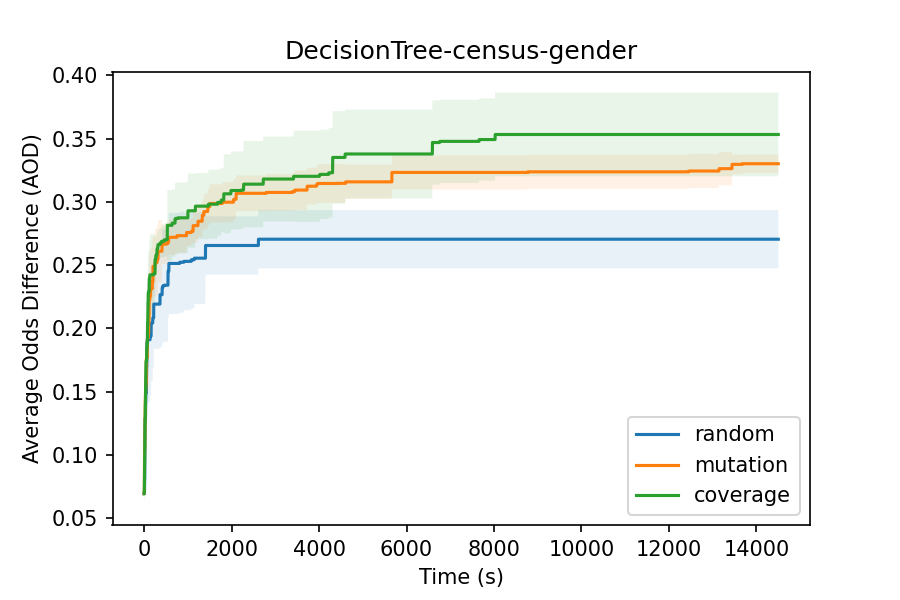
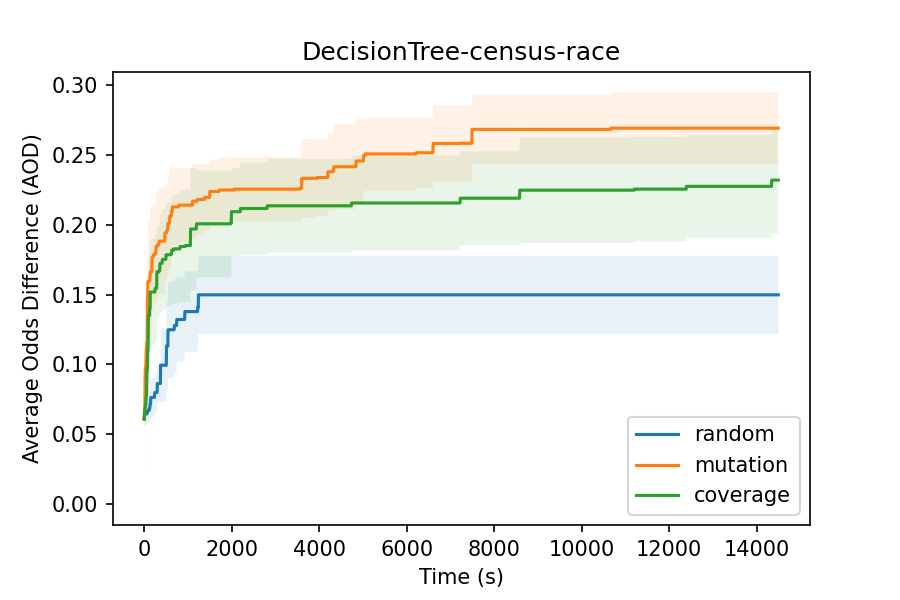
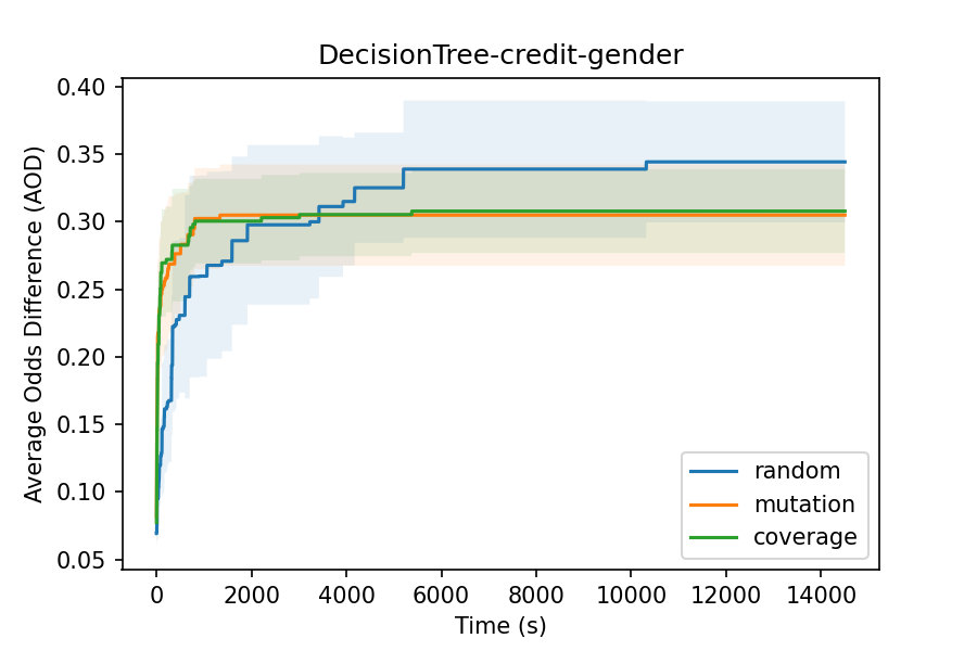
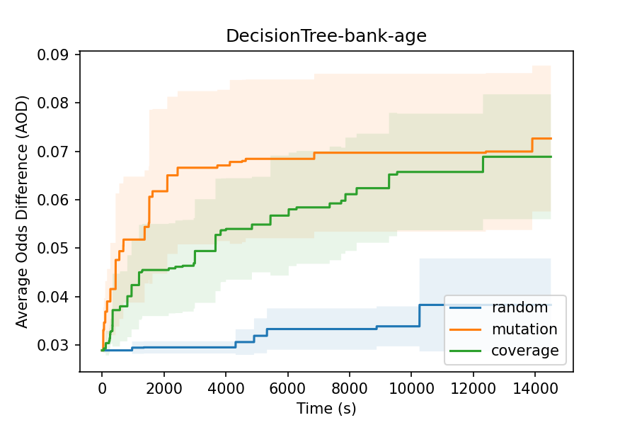
Figure 3. The temporal progress of search strategies for the decision tree algorithm over $4$ training tasks. X-axis is the timestamp of search from 0s to 14000s (4 hrs) and Y-axis is the group fairness metric ($AOD$). $Coverage$ refers to gray-box method.

In Table 3, we observe that the statistically significant differences are relevant to the decision tree (DT). For the algorithm, we provide the temporal progress of three search algorithms for different training scenarios (see supplementary material for the rest). Figure 3 shows the mean of maximum biases (sold line) and the $95\%$ confidence intervals (filled colors) over the $4$ hours testing campaigns of each search strategy. There is a statistically significant difference if white spaces are present between the confidence intervals.

6.6. Statistical Learning for Explanations (RQ3)

We present a statistical learning approach to explain what configurations distinguish low bias models from high bias ones. We use clustering to find different classes of biases and the CART tree classifiers to synthesize predicate functions that explain what parameters are common in the same cluster and what parameters distinguish one cluster from another. Similar techniques have been used for software performance debugging (Tizpaz-Niari et al., 2020). We limit the maximum number of clusters to $3$ and prefer $three$ clusters over $two$ clusters if and only if the corresponding classifier achieves better accuracy. We also limit the depth of CART classifiers to $3$ in order to generate succinct decision trees. We first present the explanatory models of different algorithms over each individual training scenario (e.g, $census$ dataset with $sex$). Next, we perform an aggregated analysis of learning algorithms over the $6$ different training datasets, the $3$ random search algorithms, and the $10$ repeated runs to extract what hyperparameters are frequently appearing in the explanatory models and thus suspicious of influencing fairness systematically.

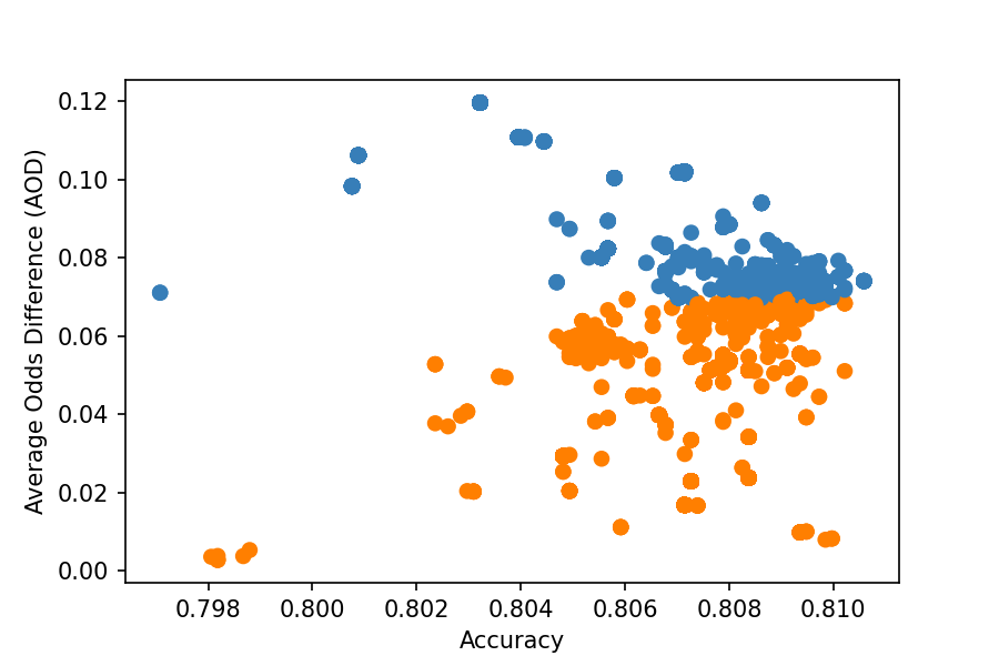
(a) Logistic Regression Cluters.

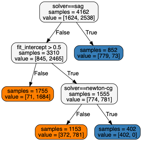
(b) Logistic Regression Explained.

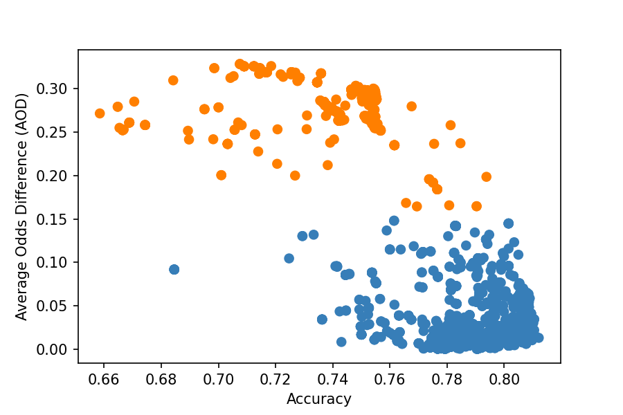
(c) SVM Clusters.

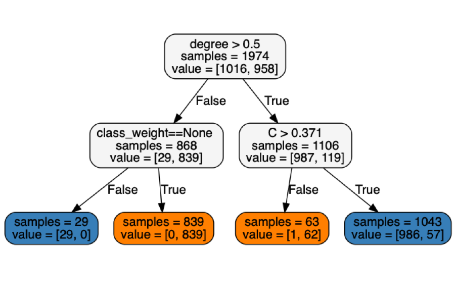
(d) SVM Explained.

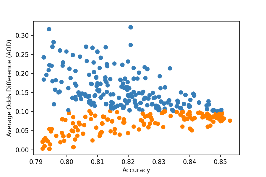
(e) Decision Tree Clusters.

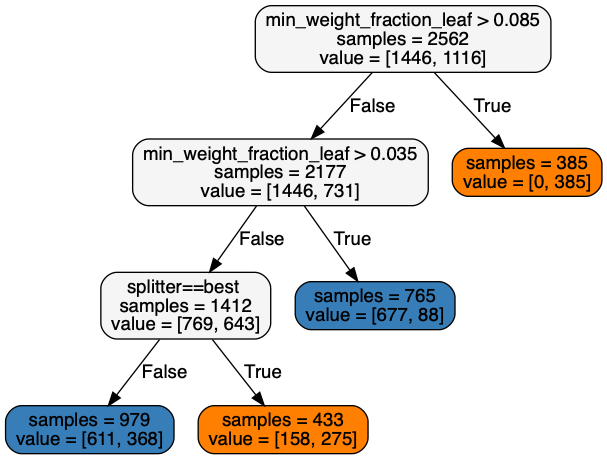
(f) Decision Tree Explained.

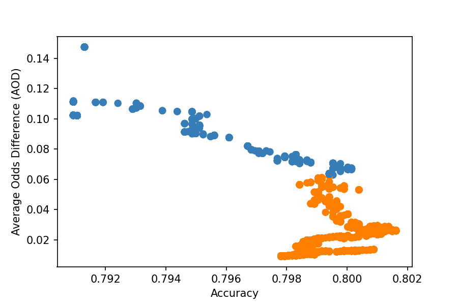
(g) Discriminant Clusters.

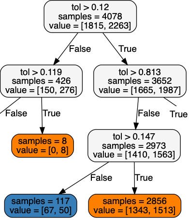
(h) Discriminant Explained.

Figure 4. The test inputs over census dataset with sex as the protected attribute are (1) clustered into two groups in the domain of fairness and accuracy (2) explained to understand which parameters distinguish low and high fairness outcomes.

Individual training scenario. We show how our statistical learning approach helps localize hyperparameters that influence the biases for each individual training task. Figure 4 shows the explanatory models (clustering and CART tree) for each learning algorithm over the $census$ dataset with $sex$ (except for random forest that was presented in the overview Section 3). For example, Figure 4 (b) shows the true evaluation of “solver!=sag $\land$ fit-intercept>0.5 $\land$ solver=newton-cg” for the hyperparameters of logistic regression, which explains the orange cluster, leads to stronger biases. All models are available in the supplementary material.

Mining over all training scenarios. For each learning algorithm, our goal is to understand what hyperparameters influence the fairness in multiple training scenarios and establish whether some hyperparameters systematically influence fairness beyond a specific training task. Overall, we analyze $180$ CART trees and report hyperparameters that appear as a node in the tree more than $50$ times overall and more than $3$ times uniquely in the $4$ datasets. Different values of these frequent hyperparameters are suspicious of introducing biases, across datasets, search algorithms, and different protected attributes. In the following, within the parenthesis right after the name of a hyperparameter, we report (1) the number of explanatory models (out of 180) where the hyperparameter appears and (2) the number of datasets (out of 4) for which there is an experiment whose explanatory model contains the hyperparameter.

A) Logistic regression (LR): The computation time for inferring clusters and tree classifiers is $77.9$ (s) in the worst case. The accuracy of classifiers is between $90.9\%$ and $96.8\%$. Three frequent hyperparameters based on the predicates in classifiers are solver (175,4), tol (53,3), and fit-intercept (50,3). Our analysis shows that the solver $saga$ frequently achieves low biases after tuning the tolerance parameter whereas the solver $newton$-$cg$ often achieves low biases if the intercept term is added to the decision function.

B) Random forest (RF): The computation time for inferring models is $75.7$ (s) in the worst case. The accuracy is between $80.5\%$ and $100.0\%$. Two frequent parameters are max_features (170,4) and min_weight_fraction_leaf (160,4). These parameters and their connections to fairness are explained in the overview section 3.

C) Support vector machine (SVM): The computation time for inferring models is $79.9$ (s) in the worst case. The accuracy is between $83.9\%$ and $98.3\%$. The only (relatively) frequent parameter is degree (53,3). This shows the high variation of parameter appearances in the explanation model. Thus, the configuration of SVM might not systematically amplify or suppress biases; the influence of configuration on biases largely depends on the specific training task.

D) Decision tree (DT): The computation time for inferring models is $76.9$ (s) in the worst case. The accuracy is between $93.8\%$ and $98.1\%$. The frequent parameters are min_fraction_leaf (114,4) and max_features (114, 4). Similar to random forest, the minimum required samples in the leaves and the search space of dataset attributes during training impact fairness systematically.

E) Discriminant analysis (DA): The computation time for inferring models is $77.8$ (s) in the worst case. The accuracy is between $54.2\%$ and $93.8\%$. However, if we allowed a higher depth for the classifier (more than $3$), it is above $90\%$ in all cases. The frequent parameter is tol (141,4). However, the exact condition over the tolerance in the explanatory model significantly depends on the training task, and might not influence fairness systematically.

ML library maintainers can use these results to understand the fairness implications of their library configurations.

6.7. Bias Mitigation Algorithms (RQ4)

Table 4. Parfait-ML as a bias mitigation technique compared to Exp. Gradient (Agarwal et al., 2018) within 6 mins.

Algorithm	Dataset	Protected	Default Configuration		Exp. Gradient (Agarwal et al., 2018)		Parfait-ML		Parfait-ML + Exp. Gradient (Agarwal et al., 2018)
			Accuracy	EOD	Accuracy	EOD	Accuracy	EOD	Accuracy	EOD
LR	Census	Sex	80.5% (+/- 0.0%)	9.7% (+/- 0.1%)	80.5% (+/- 0.1%)	0.8% (+/- 0.3%)	80.2% (+/- 0.3%)	0.1% (+/- 0.0%)	80.0% (+/- 0.5%)	0.2% (+/- 0.1%)
	Census	Race	80.5% (+/- 0.0%)	9.9% (+/- 0.0%)	79.6% (+/- 0.1%)	3.5% (+/- 2.2%)	80.2% (+/- 0.3%)	1.1% (+/- 1.0%)	80.0% (+/- 0.5%)	1.3% (+/- 0.9%)
	Credit	Sex	74.4% (+/- 0.0%)	17.1% (+/- 0.0)	74.5% (+/- 0.6%)	25% (+/- 1.9%)	75.2% (+/- 0.8%)	0.6% (+/- 0.5%)	74.3% (+/- 0.5%)	1.6% (+/- 1.2%)
	Bank	Age	89.0% (+/- 0.0%)	8.0% (+/- 0.0%)	86.7% (+/- 0.1%)	2.4% (+/- 1.6%)	88.6% (+/- 0.2%)	0.0% (+/- 0.0%)	88.2% (+/- 0.4%)	0.8% (+/- 0.8%)
	Compas	Sex	97.0% (+/- 0.0%)	1.6% (+/- 0.0%)	96.9% (+/- 0.1%)	0.0% (+/- 0.0%)	97.1% (+/- 0.0%)	0.0% (+/- 0.0%)	97.1% (+/- 0.0%)	0.0% (+/- 0.0%)
	Compas	Race	97.0% (+/- 0.0%)	0.3% (+/- 0.0%)	96.9% (+/- 0.1%)	0.0% (+/- 0.0%)	97.1% (+/- 0.0%)	0.0% (+/- 0.0%)	97.1% (+/- 0.0%)	0.0% (+/- 0.0%)
RF	Census	Sex	84.0% (+/- 0.0%)	5.4% (+/- 0.0%)	79.0% (+/- 0.0%)	5.4% (+/- 0.0%)	84.0% (+/- 0.4%)	5.0% (+/- 1.0%)	79.4% (+/- 0.0%)	0.1% (+/- 0.0%)
	Census	Race	84.0% (+/- 0.0%)	8.6% (+/- 0.0%)	79.8% (+/- 0.0%)	0.3% (+/- 0.0%)	84.7% (+/- 0.6%)	4.5% (+/- 0.5%)	79.8% (+/- 0.0%)	0.3% (+/- 0.0%)
	Credit	Sex	74.0% (+/- 0.0%)	11.6% (+/- 0.0%)	70.4% (+/- 0.0%)	8.3% (+/- 0.0%)	78.1% (+/- 0.4%)	0.1% (+/- 0.0%)	70.8% (+/- 0.0%)	0.5% (+/- 0.0%)
	Bank	Age	89.9% (+/- 0.0%)	1.2% (+/- 0.0%)	79.0% (+/- 0.3%)	3.6% (+/- 1.6%)	89.9% (+/- 0.2%)	0.1% (+/- 0.1%)	83.1% (+/- 0.8%)	0.7% (+/- 0.7%)
	Compas	Sex	96.5% (+/- 0.0%)	2.3% (+/- 0.0%)	93.6% (+/- 0.0%)	1.5% (+/- 0.0%)	97.1% (+/- 0.0%)	0.0% (+/- 0.0%)	97.1% (+/- 0.0%)	0.0% (+/- 0.0%)
	Compas	Race	96.5% (+/- 0.0%)	2.1% (+/- 0.0%)	93.7% (+/- 0.0%)	1.1% (+/- 0.0%)	97.1% (+/- 0.0%)	0.0% (+/- 0.0%)	97.1% (+/- 0.0%)	0.0% (+/- 0.0%)
SVM	Census	Sex	66.5% (+/- 0.0%)	18.5% (+/- 0.0%)	79.9% (+/- 0.0%)	0.7% (+/- 0.2%)	79.1% (+/- 0.7%)	0.0% (+/- 0.0%)	80.1% (+/- 0.4%)	0.2% (+/- 0.1%)
	Census	Race	72.5% (+/- 0.0%)	4.5% (+/- 0.0%)	72.5% (+/- 0.4%)	3.8% (+/- 1.8%)	78.8% (+/- 2.2%)	0.0% (+/- 0.0%)	76.3% (+/- 1.7%)	0.3% (+/- 0.3%)
	Credit	Sex	62.8% (+/- 0.0%)	22.3% (+/- 0.3%)	64.6% (+/- 1.7%)	10.4% (+/- 0.0%)	70.4% (+/- 0.0%)	0.0% (+/- 0.0%)	70.4% (+/- 0.0%)	0.0% (+/- 0.0%)
	Bank	Age	89.9% (+/- 0.0%)	1.2% (+/- 0.0%)	79.0% (+/- 0.3%)	3.6% (+/- 1.6%)	89.2% (+/- 0.3%)	0.0% (+/- 0.0%)	88.3% (+/- 0.1%)	0.0% (+/- 0.0%)
	Compas	Sex	96.5% (+/- 0.0%)	0.0% (+/- 0.0%)	93.6% (+/- 0.0%)	0.0% (+/- 0.0%)	97.1% (+/- 0.0%)	0.0% (+/- 0.0%)	97.1% (+/- 0.0%)	0.0% (+/- 0.0%)
	Compas	Race	96.5% (+/- 0.0%)	0.0% (+/- 0.0%)	93.7% (+/- 0.0%)	0.0% (+/- 0.0%)	97.1% (+/- 0.0%)	0.0% (+/- 0.0%)	97.1% (+/- 0.0%)	0.0% (+/- 0.0%)
DT	Census	Sex	80.2% (+/- 0.0%)	3.3% (+/- 0.0%)	82.6% (+/- 0.1%)	2.1% (+/- 0.6%)	79.9% (+/- 0.8%)	0.2% (+/- 0.2%)	82.7% (+/- 0.5%)	0.9% (+/- 1.0%)
	Census	Race	80.2% (+/- 0.0%)	7.2% (+/- 0.0%)	83.0% (+/- 0.1%)	7.5% (+/- 1.6%)	80.7% (+/- 0.9%)	0.2% (+/- 0.1%)	83.2% (+/- 0.5%)	1.7% (+/- 1.0%)
	Credit	Sex	66.0% (+/- 0.0%)	13.4% (+/- 0.0%)	70.0% (+/- 0.3%)	14.9% (+/- 1.8%)	70.4% (+/- 0.0%)	0.0% (+/- 0.0%)	70.4% (+/- 0.0%)	0.0% (+/- 0.0%)
	Bank	Age	87.1% (+/- 0.0%)	4.8% (+/- 0.0%)	88.0% (+/- 0.1%)	3.7% (+/- 1.7%)	88.4% (+/- 0.3%)	0.0% (+/- 0.0%)	88.3% (+/- 0.0%)	0.0% (+/- 0.0%)
	Compas	Sex	93.8% (+/- 0.0%)	5.2% (+/- 0.0%)	95.9% (+/- 0.0%)	2.3% (+/- 0.0%)	97.1% (+/- 0.0%)	0.0% (+/- 0.0%)	97.1% (+/- 0.0%)	0.0% (+/- 0.0%)
	Compas	Race	93.8% (+/- 0.0%)	3.8% (+/- 0.0%)	96.0% (+/- 0.0%)	1.3% (+/- 0.0%)	97.1% (+/- 0.0%)	0.0% (+/- 0.0%)	97.0% (+/- 0.1%)	0.0% (+/- 0.0%)

We show how Parfait-ML can be used as a mitigation tool to aid ML users pick a configuration of algorithms with the lowest discrimination. In doing so, we run Parfait-ML for a short amount of time and pick a configuration of hyperparameters with the lowest $AOD$ and $EOD$. To show the effectiveness, we compare Parfait-ML to the state-of-the-art techniques (Agarwal et al., 2018; Chakraborty et al., 2019, 2020). We say approach (1) outperforms approach (2) if it achieves statistically significant lower biases within a similar or higher accuracy.

A) Exponentiated gradient (Agarwal et al., 2018) presents a bias reduction technique that maximizes the prediction accuracy subject to linear constraints on the group fairness requirements. They use Lagrange methods and apply the exponentiated gradient search to find Lagrange multipliers to balance accuracy and fairness. In doing so, they use meta-learning algorithms to learn a family of classifiers (one in each step of the algorithm with a fixed Lagrange multiplier) and assign a probabilistic weight to each of them. In the prediction stage, the approach chooses one classifier from the family of classifiers stochastically according to their weights. We choose this approach for a few reasons: 1) the approach is an inprocess algorithm and does not add or remove input data samples in the pre-processing step nor modifies prediction labels in the post-processing step; 2) they assume black-box access to ML algorithms; thus they do not modify the learning objective nor model parameters. We note that their approach is sensitive to the fairness metric (to construct the linear constraints) and does not support arbitrary metrics. In particular, they support the $EOD$ metric, but not the $AOD$ metric. Thus, we focus on the $EOD$ metric in this experiment. In addition, since the discriminant analysis algorithm does not support meta-learning, we exclude this algorithm from this experiment.

We consider the default configuration of algorithms without any fairness consideration, the exponentiated gradient method (Agarwal et al., 2018), Parfait-ML, and exponentiated gradient combined with Parfait-ML. We also set the execution time of Parfait-ML to $6$ minutes in accordance with the (max) execution time of gradient approach in our environment. Table 4 shows the results of these experiments. Compared to the default configuration, in $18$ cases out of $24$ experiments, the exponentiated gradient significantly reduces the $EOD$ biases. However, in $11$ cases out of $24$ experiments, exponentiated gradient degraded the prediction accuracy. Parfait-ML reduces the $EOD$ biases in $23$ cases with $12$ cases of accuracy improvements and only one case of accuracy degradations. Overall, Parfait-ML significantly outperforms the gradient method (discrepancies are highlighted with red font in Table 4). Combining Parfait-ML and exponentiated gradient performs better than each technique in isolation (see $RF$ with $census$ and $sex$) given that the gradient technique does not increase the strength of biases in isolation (see $LR$ with $credit$ and $sex$). In such cases, Parfait-ML alone results in lower biases and higher accuracy.

Table 5. Parfait-ML in comparison to Fairway (FLASH) (Chakraborty et al., 2019, 2020).

Alg.	Scenario	Time	FLASH			Parfait-ML
		(s)	Accuracy	AOD	EOD	Accuracy	AOD	EOD
LR	Census, Sex	40.3	80.5% (+/- 0.1%)	2.0% (+/- 0.1%)	0.2% (+/- 0.3%)	80.9% (+/- 0.2%)	2.7% (+/- 1.0%)	4.3% (+/- 1.3%)
	Census,Race	65.2	80.3% (+/- 0.0%)	6.2% (+/- 0.4%)	8.0% (+/- 0.6%)	80.9% (+/- 0.0%)	4.2% (+/- 0.8%)	5.8% (+/- 1.4%)
	Credit, Sex	2.8	70.4% (+/- 0.0%)	0.0% (+/- 0.0%)	0.0% (+/- 0.0%)	76.1% (+/- 0.0%)	3.5% (+/- 0.0%)	5.5% (+/- 0.0%)
	Bank, Age	129.0	90.5% (+/- 0.0%)	0.8% (+/- 0.1%)	1.1% (+/- 0.2%)	89.6% (+/- 0.0%)	0.4% (+/- 0.2%)	0.4% (+/- 0.0%)
	Compas, Sex	18.3	97.1% (+/- 0.0%)	1.6% (+/- 0.0%)	0.0% (+/- 0.0%)	97.1% (+/- 0.0%)	1.6% (+/- 0.0%)	0.0% (+/- 0.0%)
	Compas, Race	9.5	97.1% (+/- 0.0%)	1.5% (+/- 0.0%)	0.0% (+/- 0.0%)	97.1% (+/- 0.0%)	1.5% (+/- 0.0%)	0.0% (+/- 0.0%)
DT	Census, Sex	25.8	82.5% (+/- 0.8%)	7.9% (+/- 2.2%)	9.9% (+/- 3.7%)	83.6% (+/- 0.8%)	4.8% (+/- 1.1%)	2.2% (+/- 0.5%)
	Census, Race	60.5	83.9% (+/- 0.7%)	3.2% (+/- 1.0%)	4.3% (+/- 1.8%)	84.1% (+/- 0.8%)	3.1% (+/- 1.1%)	4.4% (+/- 1.6%)
	Credit, Sex	2.5	71.5% (+/- 1.3%)	5.4% (+/- 2.2%)	7.7% (+/- 4.2%)	71.1% (+/- 0.0%)	0.0% (+/- 0.0%)	0.0% (+/- 0.0%)
	Bank, Age	124.8	90.9% (+/- 0.1%)	0.7% (+/- 0.4%)	0.8% (+/- 0.8%)	88.9% (+/- 0.4%)	0.0% (+/- 0.0%)	5.6% (+/- 0.0%)
	Compas, Sex	5.9	97.1% (+/- 0.0%)	1.6% (+/- 0.0%)	0.0% (+/- 0.0%)	97.1% (+/- 0.0%)	1.5% (+/- 0.2%)	0.0% (+/- 0.0%)
	Compas, Race	11.4	97.1% (+/- 0.0%)	1.5% (+/- 0.0%)	0.0% (+/- 0.0%)	97.1% (+/- 0.0%)	1.5% (+/- 0.0%)	0.0% (+/- 0.0%)

B) Fairway (Chakraborty et al., 2019, 2020) uses a mutli-objective optimization technique known as FLASH (Nair et al., 2020) to tune hyperparameters and chooses a configuration that achieves less biases with a minimum accuracy loss. We use their implementatio (Chakraborty et al., 2021), and compare our search-based technique to this method. Fairway generally supports integer and boolean hyperparameters. Therefore, we use a subset of configurations as specified and reported for logistic regression (LR) (Chakraborty et al., 2020) and decision tree (DT) (Chakraborty et al., 2019). For a fair comparison, we calculate the execution time of Fairway for each experiment in our environment and limit the execution time of Parfait-ML accordingly. Table 5 shows the comparison results. Overall, there are $3$ discrepancies in AOD and $5$ discrepancies in EOD (noted by red font in Table 5). Parfait-ML outperforms Fairway in $6$ cases whereas Fairway outperforms Parfait-ML in $2$ cases. We also noted that the current implementations of FLASH carefully selected $4$ hyperparameters for LR and DT. When we include three more hyperparameters with integer or boolean types (e.g., dual and fit_intercept in $LR$), we observe that the performance of Fairway significantly degraded. For $LR$ algorithm over $compas$ with $sex$ scenario, the prediction accuracy is decreased to $89.7\%(+/-6.0\%)$, while the AOD and EOD bias metrics are increased to $2.9\%(+/-1.0\%)$ and $3.1\%(+/-2.3\%)$, respectively. Since Fairway is sensitive to the domain of variables, Parfait-ML can complement it with the explanatory model to carefully choose hyperparameters to include in the Fairway search.

7. Discussion

Limitation. The input dataset is arguably the main source of discriminations in data-driven software. In this work, we vary the configuration of learning algorithms and fix the input dataset since our approach is to systematically study the influence of hyperparameters in fairness. While we found that configurations can reduce biases in various algorithms, our approach alone cannot eliminate fairness bugs. Our approach also requires a diverse set of inputs generated automatically using the search algorithms. As a dynamic analysis, our approach solely relies on heuristics to generate a diverse set of configurations and is not guaranteed to always find interesting hyperparameters in a given time limit. In addition, we only use two group fairness metrics ($AOD$ and $EOD$) and the overall prediction accuracy. One limitation is that these metrics do not consider the distribution of different groups. In general, coming up with a suitable fairness definition is an open challenge.

Threat to Validity. To address the internal validity and ensure our finding does not lead to invalid conclusion, we follow established guideline (Arcuri and Briand, 2014) where we repeat every experiment $10$ times, report the average with $95\%$ confidence intervals (CI), and consider not only the final result but also the temporal progresses. We note that $95\%$ non-overlapping CI is a conservative statistical method to compare results. Instead, non-parametric methods and effect sizes can be used to alleviate the conservativeness of our comparisons. In our experiments, we did not find significant improvements using coverage metrics. However, this might be a result of our specific implementations and/or the feedback criteria. To ensure that our results are generalizable and address external validity, we perform our experiments on five learning algorithms from scikit-learn library over six fairness-sensitive applications that have been widely used in the fairness literature. However, it is an open problem whether the library, algorithms, and applications are sufficiently representative to cover challenging fairness scenarios.

Usage Vision. Parfait-ML complements the workflow of standard testing procedures against functionality and performance by enabling ML library maintainers to detect and debug fairness bugs. Parfait-ML combines search-based software testing with statistical debugging to identify and explain hyperparameters that lead to high and low bias classifiers within acceptable accuracy. Like standard ML code testing, Parfait-ML requires a set of reference fairness-sensitive datasets. If the explanatory models are consistent across these datasets, Parfait-ML synthesizes this information to pinpoint dataset-agnostic fairness bugs. If such bugs are discovered, ML library maintainers can either exclude those options or warn users to avoid setting them for fairness-sensitive applications.

8. Conclusion

Software developers increasingly employ machine learning libraries to design data-driven social-critical applications that demand a delicate balance between accuracy and fairness. The “programming” task in designing such systems involves carefully selecting hyperparameters for these libraries, often resolved by rules-of-thumb. We propose a search-based software engineering approach to exploring the space of hyperparameters to approximate the twined Pareto curves expressing both high and low fairness against accuracy. Hyperparameter configurations with high fairness help software engineers mitigate bias, while configurations with low fairness help ML developers understand and document potentially unfair combinations of hyperparameters. There are multiple exciting future directions. For example, extending our methodology to support deep learning frameworks is an interesting future work.

- (1)
- Agarwal et al. (2018) Alekh Agarwal, Alina Beygelzimer, Miroslav Dudík, John Langford, and Hanna Wallach. 2018. A reductions approach to fair classification. In International Conference on Machine Learning. PMLR, 60–69.
- Aggarwal et al. (2019) Aniya Aggarwal, Pranay Lohia, Seema Nagar, Kuntal Dey, and Diptikalyan Saha. 2019. Black Box Fairness Testing of Machine Learning Models. In Proceedings of the 2019 27th ACM Joint Meeting on European Software Engineering Conference and Symposium on the Foundations of Software Engineering (ESEC/FSE 2019). 625–635. https://doi.org/10.1145/3338906.3338937
- Arcuri and Briand (2014) Andrea Arcuri and Lionel Briand. 2014. A Hitchhiker’s guide to statistical tests for assessing randomized algorithms in software engineering. Software Testing, Verification and Reliability (2014), 219–250. https://doi.org/10.1002/stvr.1486
- Bellamy et al. (2019) Rachel KE Bellamy, Kuntal Dey, Michael Hind, Samuel C Hoffman, Stephanie Houde, Kalapriya Kannan, Pranay Lohia, Jacquelyn Martino, Sameep Mehta, Aleksandra Mojsilović, et al. 2019. AI Fairness 360: An extensible toolkit for detecting and mitigating algorithmic bias. IBM Journal of Research and Development 63, 4/5 (2019), 4–1.
- Blumrosen (1978) Ruth G Blumrosen. 1978. Wage discrimination, job segregation, and the title vii of the civil rights act of 1964. U. Mich. JL Reform 12 (1978), 397.
- Breiman et al. (1984) L. Breiman, J.H. Friedman, R.A. Olshen, and C.I. Stone. 1984. Classification and regression trees. Wadsworth: Belmont, CA.
- Brun and Meliou (2018) Yuriy Brun and Alexandra Meliou. 2018. Software Fairness (ESEC/FSE 2018). 754–759. https://doi.org/10.1145/3236024.3264838
- Chakraborty et al. (2020) Joymallya Chakraborty, Suvodeep Majumder, Zhe Yu, and Tim Menzies. 2020. Fairway: a way to build fair ML software. In Proceedings of the 28th ACM Joint Meeting on European Software Engineering Conference and Symposium on the Foundations of Software Engineering. 654–665.
- Chakraborty et al. (2021) Joymallya Chakraborty, Suvodeep Majumder, Zhe Yu, and Tim Menzies. 2021. implementation of Fairway. https://github.com/joymallyac/Fairway. Online.
- Chakraborty et al. (2019) Joymallya Chakraborty, Tianpei Xia, Fahmid M. Fahid, and Tim Menzies. 2019. Software Engineering for Fairness: A Case Study with Hyperparameter Optimization. arXiv:1905.05786
- Deb et al. (2002) Kalyanmoy Deb, Amrit Pratap, Sameer Agarwal, and TAMT Meyarivan. 2002. A fast and elitist multiobjective genetic algorithm: NSGA-II. IEEE transactions on evolutionary computation 6, 2 (2002), 182–197.
- Deloitte (2021) Deloitte. 2021. Better Data, Faster Delivery, Actionable Insights. https://www2.deloitte.com/us/en/pages/deloitte-analytics/solutions/insuresense-insurance-data-analytics-platform-data-management-services.html. Online.
- Dua and Graff (2017a) Dheeru Dua and Casey Graff. 2017a. UCI Machine Learning Repository. https://archive.ics.uci.edu/ml/datasets/census+income
- Dua and Graff (2017b) Dheeru Dua and Casey Graff. 2017b. UCI Machine Learning Repository. https://archive.ics.uci.edu/ml/datasets/statlog+(german+credit+data)
- Dua and Graff (2017c) Dheeru Dua and Casey Graff. 2017c. UCI Machine Learning Repository. https://archive.ics.uci.edu/ml/datasets/bank+marketing
- Dwork et al. (2012) Cynthia Dwork, Moritz Hardt, Toniann Pitassi, Omer Reingold, and Richard Zemel. 2012. Fairness through awareness. In Proceedings of the 3rd innovations in theoretical computer science conference. 214–226.
- Galhotra et al. (2017) Sainyam Galhotra, Yuriy Brun, and Alexandra Meliou. 2017. Fairness Testing: Testing Software for Discrimination (ESEC/FSE 2017). Association for Computing Machinery, New York, NY, USA. https://doi.org/10.1145/3106237.3106277
- Hardt et al. (2016) Moritz Hardt, Eric Price, and Nati Srebro. 2016. Equality of Opportunity in Supervised Learning. In NIPS.
- Julia Angwin and Kirchne (2021) Surya Mattu Julia Angwin, Jeff Larson and Lauren Kirchne. 2021. Machine Bias. https://www.propublica.org/article/machine-bias-risk-assessments-in-criminal-sentencing. Online.
- Kamiran et al. (2012) Faisal Kamiran, Asim Karim, and Xiangliang Zhang. 2012. Decision Theory for Discrimination-Aware Classification. In 2012 IEEE 12th International Conference on Data Mining. 924–929. https://doi.org/10.1109/ICDM.2012.45
- Kampmann et al. (2020) Alexander Kampmann, Nikolas Havrikov, Soremekun Ezekiel, and Andreas Zeller. 2020. When does my Program do this? Learning Circumstances of Software Behavior (FSE 2020).
- Kuhn et al. (2013) Max Kuhn, Kjell Johnson, et al. 2013. Applied predictive modeling. Vol. 26. Springer.
- Nair et al. (2020) Vivek Nair, Zhe Yu, Tim Menzies, Norbert Siegmund, and Sven Apel. 2020. Finding Faster Configurations Using FLASH. IEEE Transactions on Software Engineering 46, 7 (2020), 794–811. https://doi.org/10.1109/TSE.2018.2870895
- Northpointe (2012) Northpointe. 2012. Practitioners Guide to COMPAS. http://www.northpointeinc.com/files/technical_documents/FieldGuide2_081412.pdf. Online.
- O’Whielacronx (2018) Zooko O’Whielacronx. 2018. A program/module to trace Python program or function execution. https://docs.python.org/3/library/trace.html. Online.
- ProPublica (2021) ProPublica. 2021. Compas Software Ananlysis. https://github.com/propublica/compas-analysis. Online.
- scikit learn (2021a) scikit learn. 2021a. Decision Tree Classifier. https://scikit-learn.org/stable/modules/generated/sklearn.tree.DecisionTreeClassifier.html. Online.
- scikit learn (2021b) scikit learn. 2021b. Discriminant Analysis. https://scikit-learn.org/stable/modules/lda_qda.html. Online.
- scikit learn (2021c) scikit learn. 2021c. Logistic Regression. https://scikit-learn.org/stable/modules/generated/sklearn.linear_model.LogisticRegression.html. Online.
- scikit learn (2021d) scikit learn. 2021d. Random Forest Regressor. https://scikit-learn.org/stable/modules/generated/sklearn.ensemble.RandomForestRegressor.html. Online.
- scikit learn (2021e) scikit learn. 2021e. Support Vector Machine. https://scikit-learn.org/stable/modules/generated/sklearn.svm.LinearSVC.html. Online.
- Scism and Maremont (2010) Leslie Scism and Mark Maremont. 2010. Insurers test data profiles to identify risky clients. https://www.wsj.com/articles/SB10001424052748704648604575620750998072986. Online.
- Tizpaz-Niari et al. (2018) Saeid Tizpaz-Niari, Pavol Cerný, Bor-Yuh Evan Chang, and Ashutosh Trivedi. 2018. Differential Performance Debugging With Discriminant Regression Trees. In Proceedings of the Thirty-Second AAAI Conference on Artificial Intelligence (AAAI-18). 2468–2475. https://www.aaai.org/ocs/index.php/AAAI/AAAI18/paper/view/16647
- Tizpaz-Niari et al. (2020) Saeid Tizpaz-Niari, Pavol Černý, and Ashutosh Trivedi. 2020. Detecting and Understanding Real-World Differential Performance Bugs in Machine Learning Libraries (ISSTA). https://doi.org/10.1145/3395363.3404540
- Udeshi et al. (2018) Sakshi Udeshi, Pryanshu Arora, and Sudipta Chattopadhyay. 2018. Automated directed fairness testing. In Proceedings of the 33rd ACM/IEEE International Conference on Automated Software Engineering. 98–108.
- Von Luxburg (2007) Ulrike Von Luxburg. 2007. A tutorial on spectral clustering. Statistics and computing 17, 4 (2007), 395–416.
- Zeller et al. (2021) Andreas Zeller, Rahul Gopinath, Marcel Böhme, Gordon Fraser, and Christian Holler. 2021. The Fuzzing Book. CISPA Helmholtz Center for Information Security. https://www.fuzzingbook.org/ Retrieved 2021-10-26 15:30:20+02:00.
- Zhang et al. (2018) Brian Hu Zhang, Blake Lemoine, and Margaret Mitchell. 2018. Mitigating unwanted biases with adversarial learning. In Proceedings of the 2018 AAAI/ACM Conference on AI, Ethics, and Society. 335–340.
- Zhang and Harman (2021) Jie M. Zhang and Mark Harman. 2021. ”Ignorance and Prejudice” in Software Fairness. In 43rd IEEE/ACM International Conference on Software Engineering, ICSE 2021, Madrid, Spain, 22-30 May 2021. IEEE, 1436–1447. https://doi.org/10.1109/ICSE43902.2021.00129
- Zhang et al. (2020a) Jie M Zhang, Mark Harman, Lei Ma, and Yang Liu. 2020a. Machine learning testing: Survey, landscapes and horizons. IEEE Transactions on Software Engineering (2020).
- Zhang et al. (2020b) Peixin Zhang, Jingyi Wang, Jun Sun, Guoliang Dong, Xinyu Wang, Xingen Wang, Jin Song Dong, and Ting Dai. 2020b. White-Box Fairness Testing through Adversarial Sampling (ICSE ’20). Association for Computing Machinery, New York, NY, USA. https://doi.org/10.1145/3377811.3380331