Metadata-Induced Contrastive Learning for
Zero-Shot Multi-Label Text Classification

Abstract.

Large-scale multi-label text classification (LMTC) aims to associate a document with its relevant labels from a large candidate set. Most existing LMTC approaches rely on massive human-annotated training data, which are often costly to obtain and suffer from a long-tailed label distribution (i.e., many labels occur only a few times in the training set). In this paper, we study LMTC under the zero-shot setting, which does not require any annotated documents with labels and only relies on label surface names and descriptions. To train a classifier that calculates the similarity score between a document and a label, we propose a novel metadata-induced contrastive learning (MICoL) method. Different from previous text-based contrastive learning techniques, MICoL exploits document metadata (e.g., authors, venues, and references of research papers), which are widely available on the Web, to derive similar document–document pairs. Experimental results on two large-scale datasets show that: (1) MICoL significantly outperforms strong zero-shot text classification and contrastive learning baselines; (2) MICoL is on par with the state-of-the-art supervised metadata-aware LMTC method trained on 10K–200K labeled documents; and (3) MICoL tends to predict more infrequent labels than supervised methods, thus alleviates the deteriorated performance on long-tailed labels.

1. Introduction

Large-scale multi-label text classification (LMTC) (Chalkidis et al., 2019) aims to find the most relevant labels to an input document given a large collection of candidate labels. As a fundamental task in text mining, LMTC has many Web-related applications such as product keyword recommendation on Amazon (Chang et al., 2020), academic paper classification on Microsoft Academic and PubMed (Zhang et al., 2021c), and article tagging on Wikipedia (Jain et al., 2016).

Most previous attempts address LMTC in a supervised fashion (Agrawal et al., 2013; Jain et al., 2016; Prabhu et al., 2018; You et al., 2019; Jain et al., 2019; Liu et al., 2017; Yen et al., 2017; Medini et al., 2019; Chang et al., 2020; Zhang et al., 2021c; Saini et al., 2021; Mittal et al., 2021), where the proposed text classifiers are trained on a large set of human-annotated documents. While achieving inspiring performance, these approaches have three limitations. First, obtaining enough human-labeled training data is often expensive and time-consuming, especially when the label space is large. Second, the trained classifiers can only predict labels they have seen in the training set. When new categories (e.g., “COVID-19”) emerge, the classifiers need to be re-trained. Third, the label distribution is often imbalanced in LMTC. Several labels (e.g., “World Wide Web”) have numerous training samples, while many others (e.g., “Bipartite Ranking”) occur only a few times. Related studies (Wei and Li, 2018; Wei et al., 2021) have shown that supervised approaches tend to predict frequent labels and overlook long-tailed ones.

(a) Label “Webgraph” from Microsoft Academic (https://academic.microsoft.com/topic/2777569578/).

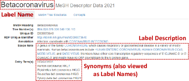
(b) Label “Betacoronavirus” from PubMed (https://meshb.nlm.nih.gov/record/ui?ui=D000073640).

Figure 1. Two examples of labels with name(s) and description from Microsoft Academic (Wang et al., 2020b) and PubMed (Lu, 2011).

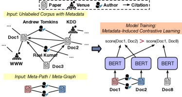
(a) Training phase of MICoL.

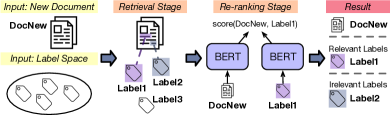
(b) Inference phase of MICoL.

Figure 2. Overview of the proposed MICoL framework.

Being aware of the annotation cost and frequent emergence of new labels, some studies (Chalkidis et al., 2019; Gupta et al., 2021; Nam et al., 2015; Rios and Kavuluru, 2018) focus on zero-shot LMTC. In their settings, annotated training documents are given for a set of seen classes, and they are tasked to build a classifier to predict unseen classes. However, as indicated in (Yin et al., 2019), we often face a more challenging scenario in real-world settings: all labels are unseen; we do not have any training samples with labels. For example, on Microsoft Academic (Wang et al., 2020b), all labels are scientific concepts extracted from research publications on the Web (Shen et al., 2018), thus no annotated training data is available when the label space is created. Motivated by such applications, in this paper, we study zero-shot LMTC with a completely new label space. The only signal we use to characterize each label is its surface name and description. Figure 1 shows two examples of label information from Microsoft Academic (Wang et al., 2020b) and PubMed (Lu, 2011).

Although relevant labels are not available for documents, there is another type of information widely available on the Web but less concerned in previous studies: document metadata. We take scientific papers as an example: in addition to text information (e.g., title and abstract), a paper is also associated with various metadata fields such as its authors, venue, and references. As shown in Figure 2(a), a heterogeneous network (Sun and Han, 2012) can be constructed to interconnect papers via their metadata information: papers, authors, and venues are nodes; authored-by, published-in, and cited-by are edges. Such metadata information could be strong label indicators of a paper. For example, in Figure 2(a), the venue node WWW suggests Doc1’s relevance to “World Wide Web”. Moreover, metadata could also imply that two papers share common labels. For example, we know Doc1 and Doc2 may have similar research topics because they are co-authored by Andrew Tomkins and Ravi Kumar or they are co-cited by Doc3. More generally, metadata also exist in Web content such as e-commerce reviews (e.g., reviewer and product information) (Zhang et al., 2021d), social media posts (e.g., users and hashtags) (Zhang et al., 2017), and code repositories (e.g., contributors) (Zhang et al., 2019). Although metadata have been used in fully supervised (Zhang et al., 2021c) or single-label (Zhang et al., 2020; Mekala et al., 2020; Zhang et al., 2021d, b) text classification, it is largely unexplored in zero-shot LMTC.

Contributions. In this paper, we propose a novel metadata-induced contrastive learning (MICoL) framework for zero-shot LMTC. To perform classification, the key module in our framework is to compute a similarity score between two text units (i.e., one document and one label name/description) so that we can produce a rank list of relevant labels for each document. Without annotated document–label pairs to train the similarity scorer, we leverage metadata to generate similar document–document pairs. Inspired by the idea of contrastive learning (Chen et al., 2020), we train the scorer by pulling similar document closer while pushing dissimilar ones apart. For example, in Figure 2(a), we assume two papers sharing at least two authors are similar (this can be described by the notion of meta-paths (Sun et al., 2011b) and meta-graphs (Zhang et al., 2018), which will be formally introduced in Section 2.1). The similarity scorer is trained to score (Doc1, Doc2) higher than (Doc1, Doc8), where Doc8 is a randomly sampled paper. In the inference phase, as shown in Figure 2(b), we first use a discrete retriever (e.g., BM25 (Robertson and Walker, 1994)) to select a set of candidate labels from the large label space. Next, we utilize the trained scorer to re-rank candidate labels to obtain the final classification results. Note that label information is only used during inference, thus no re-training is required when new labels emerge.

We demonstrate the effectiveness of MICoL on two datasets (Zhang et al., 2021c) extracted from Microsoft Academic (Wang et al., 2020b) and PubMed (Lu, 2011), both with more than 15K labels. The results indicate that: (1) MICoL significantly outperforms strong zero-shot LMTC (Yin et al., 2019) and contrastive learning (Wei and Zou, 2019; Xie et al., 2020; Cohan et al., 2020) baselines. (2) When we use P@$k$ and NDCG@$k$ as evaluation metrics, MICoL is competitive with the state-of-the-art supervised metadata-aware LMTC algorithm (Zhang et al., 2021c) trained on 10K–50K labeled documents; (3) When it is evaluated by metrics promoting correct prediction on tail labels (Jain et al., 2016; Wei et al., 2021), MICoL is on par with the supervised method trained on 100K–200K labeled documents. This demonstrates that MICoL tends to predict more infrequent labels than supervised methods, thus alleviates the deteriorated performance on tail labels.

To summarize, this work makes the following contributions:

• We propose a zero-shot LMTC framework that utilizes document metadata. The framework does not require any labeled training data and only relies on label surface names and descriptions during inference.

• We propose a novel metadata-induced contrastive learning method. Different from previous contrastive learning approaches (Giorgi et al., 2021; Wu et al., 2020; Luo et al., 2021; Gao et al., 2021b; Yan et al., 2021) which manipulate text only, we exploit metadata information to produce contrastive training pairs.

• We conduct extensive experiments on two large-scale datasets to demonstrate the effectiveness of the proposed MICoL framework.

2. Preliminaries

2.1. Metadata, Meta-Path, and Meta-Graph

Metadata. Documents on the Web are usually accompanied by rich metadata information (Zhang et al., 2020; Mekala et al., 2020; Zhang et al., 2021c). To provide a holistic view of documents with metadata, we can construct a heterogeneous information network (HIN) (Sun and Han, 2012) to connect documents together.

Definition 2.1.

(Heterogeneous Information Network (Sun and Han, 2012)) An HIN is a graph $G=(\mathcal{V},\mathcal{E})$ with a node type mapping $\phi:\mathcal{V}\rightarrow\mathcal{T}_{\mathcal{V}}$ and an edge type mapping $\psi:\mathcal{E}\rightarrow\mathcal{T}_{\mathcal{E}}$. Either the number of node types $|\mathcal{T}_{\mathcal{V}}|$ or the number of edge types $|\mathcal{T}_{\mathcal{E}}|$ is larger than 1.

As shown in Figure 2(a), in our constructed HIN, each document is a node, and each metadata field is described by either a node (e.g., author, venue) or an edge (e.g., reference).

Meta-Path. With the constructed HIN, we are able to analyze various relations between documents. Due to network heterogeneity, two documents can be connected via different paths. For example, when two papers share a common author, they can be connected via “paper–author–paper”; when one paper cites the other, they can also be connected via “paper$\rightarrow$paper”. To capture the proximity between two nodes from different semantic perspectives, meta-paths (Sun et al., 2011b) are extensively used in HIN studies.

Definition 2.2.

(Meta-Path (Sun et al., 2011b)) A meta-path is a path $\mathcal{M}$ defined on the graph $T_{G}=(\mathcal{T}_{\mathcal{V}},\mathcal{T}_{\mathcal{E}})$, and is denoted in the form of $\mathcal{M}=V_{1}\xrightarrow{E_{1}}V_{2}\xrightarrow{E_{2}}\cdots\xrightarrow{E_{m-1}}V_{m}$, where $V_{1},...,V_{m}$ are node types and $E_{1},...,E_{m-1}$ are edge types.

Each node is abstracted by its type in a meta-path, and a meta-path describes a composite relation between node types $V_{1}$ and $V_{m}$. Figures 3(a) and 3(b) show two examples of meta-paths. Following previous studies (Sun et al., 2011b; Dong et al., 2017), we use initial letters to represent node types (e.g., $P$ for paper, $A$ for author) and omit the edge types when there is no ambiguity. The two meta-paths in Figures 3(a) and 3(b) can be written as $PAP$ and $P\rightarrow P\leftarrow P$, respectively.

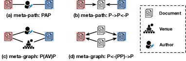
Figure 3. Examples of meta-paths and meta-graphs. Each meta-path/meta-graph describes one type of relation between the red paper and the blue paper.

Meta-Graph. In some cases, paths may not be sufficient to capture latent semantics between two nodes. For example, one meta-path cannot describe the relation between two papers that share at least two authors. Note that this relation is worth studying because two co-authors can be more informative than a single author when we infer semantic similarities between papers. Allegedly, one researcher may work on multiple topics during his/her career, while the collaboration between two researchers often focuses on a specific direction. Meta-graphs (Zhang et al., 2018) are proposed to depict such complex relations in an HIN.

Definition 2.3.

(Meta-Graph (Zhang et al., 2018)) A meta-graph is a directed acyclic graph (DAG) $\mathcal{M}$ defined on $T_{G}=(\mathcal{T}_{\mathcal{V}},\mathcal{T}_{\mathcal{E}})$. It has a single source node $V_{1}$ and a single target node $V_{m}$. Each node in $\mathcal{M}$ is a node type and each edge in $\mathcal{M}$ is an edge type.

Figures 3(c) and 3(d) give two examples of meta-graphs. Figure 3(c) describes two papers sharing the same venue and one common author, while Figure 3(d) shows two papers both cited by another two shared papers. Similar to the notation of meta-paths, we denote them as $P(AV)P$ and $P\leftarrow(PP)\rightarrow P$.

Reachability. We assume that two documents connected via a certain meta-path/meta-graph share similar topics. Formally, we introduce the concept of “reachable”.

Definition 2.4.

(Reachable) Given a meta-path/meta-graph $\mathcal{M}$ and two documents $d_{1},d_{2}$, we say $d_{2}$ is reachable from $d_{1}$ via $\mathcal{M}$ if and only if we can find a path/DAG $\mathcal{M}_{0}$ in the HIN such that: (1) $d_{1}$ is the source node of $\mathcal{M}_{0}$; (2) $d_{2}$ is the target node of $\mathcal{M}_{0}$; (3) when each node in $\mathcal{M}_{0}$ is abstracted by its node type, $\mathcal{M}_{0}$ becomes $\mathcal{M}$.

We use $d_{1}\rightarrow^{\mathcal{M}}d_{2}$ to denote that $d_{2}$ is reachable from $d_{1}$ via $\mathcal{M}$, and we use $\mathcal{N}_{\mathcal{M}}(d_{1})$ to denote the set of nodes that are reachable from $d_{1}$ (i.e., $\mathcal{N}_{\mathcal{M}}(d_{1})=\{d_{2}\ |\ d_{1}\rightarrow^{\mathcal{M}}d_{2},\ d_{2}\neq d_{1}\}$).

2.2. Problem Definition

Zero-shot multi-label text classification (Wang et al., 2019b) aims to tag each document with labels that are unseen during training time but available for prediction. Most previous studies (Rios and Kavuluru, 2018; Chalkidis et al., 2019; Gupta et al., 2021; Nam et al., 2015) assume that there is a set of seen classes, each of which has some annotated documents. Trained on these documents, their proposed text classifiers are expected to transfer the knowledge from seen classes to the prediction of unseen ones.

In this paper, we study a more challenging setting (proposed in (Yin et al., 2019) previously), where all labels are unseen. In other words, given the label space $\mathcal{L}$, we do not have any training sample for $l\in\mathcal{L}$. Instead, we assume a large-scale unlabeled corpus $\mathcal{D}$ is given, and each document $d\in\mathcal{D}$ is associated with metadata information. As mentioned in Section 2.1, with such metadata, we can construct an HIN $G=(\mathcal{V},\mathcal{E})$ to describe the relations between documents. We aim to train a multi-label text classifier $f$ based on both the text information $\mathcal{D}$ and the network information $G$. As an inductive task, the classifier $f$ needs to predict its relevant labels given a new document $d\notin\mathcal{D}$.

Since no training data is available to characterize a given label, same as previous studies (Rios and Kavuluru, 2018; Yin et al., 2019), we assume each label $l$ has some text information to describe its semantics, such as label names $n_{l}$ (Yin et al., 2019; Shen et al., 2021) and descriptions $s_{l}$ (Chang et al., 2020; Chai et al., 2020). Examples of such label information have been shown in Figure 1. To summarize, our task can be formally defined as follows:

Definition 2.5.

(Problem Definition) Given an unlabeled corpus $\mathcal{D}$ with metadata information $G=(\mathcal{V},\mathcal{E})$, and a label space $\mathcal{L}$ with label names and descriptions $\{n_{l},s_{l}|l\in\mathcal{L}\}$, our task is to learn a multi-label text classifier $f$ that can map a new document $d\notin\mathcal{D}$ to its relevant labels $\mathcal{L}_{d}\subseteq\mathcal{L}$.

3. The MICoL Framework

3.1. A Two-Stage Framework

As shown in Figure 2(b), in the proposed MICoL framework, the LMTC problem is formulated as a ranking task. Specifically, given a new document (i.e., the “query”), our task is to predict top-ranked labels (i.e., the “items”) that are relevant to the document. Note that in LMTC, the label space $\mathcal{L}$ (i.e., the “item pool”) is large. For example, in both the Microsoft Academic and PubMed datasets (Zhang et al., 2021c), there are more than 15,000 labels. Given a large item pool, recent ranking approaches are usually pipelined (Nogueira et al., 2019; Gao et al., 2021a), consisting of a first-stage discrete retriever (e.g., BM25 (Robertson and Walker, 1994)) that efficiently generates a set of candidate items followed by a continuous re-ranker (e.g., BERT (Devlin et al., 2019)) that selects the most promising items from the candidates. Such design is a natural choice due to the effectiveness-efficiency trade-off among different ranking models: discrete rankers based on lexical matching are faster but less accurate; continuous rankers can perform latent semantic matching but are much slower.

Following such prevalent approaches, MICoL adopts a two-stage ranking framework, with a discrete retrieval stage and a continuous re-ranking stage. The major novelty of MICoL is that, with document metadata information, a new contrastive learning method is developed to significantly improve the re-ranking stage performance upon BERT-based models.

3.2. The Retrieval Stage

Since the main goal of this paper is to develop a novel contrastive learning framework for re-ranking, we do not aim at a complicated design of the retrieval stage. Therefore, we adopt two simple strategies: exact name matching and sparse retrieval.

Exact Name Matching. Given a document $d$ and a label $l$, if the label name $n_{l}$ appears in the document text, we add $l$ as a candidate of $d$’s relevant labels. We use $\mathcal{C}_{\rm exact}(d)$ to denote the set of candidate labels obtained by exact name matching.

Sparse Retrieval. We cannot expect all relevant labels of a document explicitly appear in its text. To increase the recall of our retrieval stage, we adopt BM25 (Robertson and Walker, 1994) to allow partial lexical matching between documents and labels. Specifically, we concatenate the name and the description together as the text information $t_{l}$ of each label (i.e., $t_{l}=n_{l}\ ||\ s_{l}$). Then, the score between $d$ and $l$ is calculated as

(1) $${\rm BM25}(d,l)=\sum_{w\in d\cap t_{l}}{\rm IDF}(w)\frac{{\rm TF}(w,t_{l})\cdot(k_{1}+1)}{{\rm TF}(w,t_{l})\cdot k_{1}(1-b+b\frac{|\mathcal{L}|}{avgdl})}.$$

Here, $k_{1}=1.5$ and $b=0.75$ are parameters of BM25; $avgdl=\frac{1}{|\mathcal{L}|}\sum_{l\in\mathcal{L}}|t_{l}|$ is the average length of label text information. Note that in classification tasks, documents are “queries” and labels are “items” being ranked. When the BM25 score between $d$ and $l$ exceeds a certain threshold $\eta$, we add $l$ as a candidate of $d$’s relevant labels. Formally,

(2) $$\mathcal{C}_{\rm BM25}(d)=\{l\ |\ l\in\mathcal{L},\ {\rm BM25}(d,l)>\eta\}.$$

Given a document $d$, its candidate label set $\mathcal{C}(d)=\mathcal{C}_{\rm exact}(d)\cup\mathcal{C}_{\rm BM25}(d)$ (i.e., the union of candidates obtained by exact name matching and by sparse retrieval).

3.3. The Re-ranking Stage

Encouraged by the success of BERT (Devlin et al., 2019) in a wide range of text mining tasks, we build our re-ranker upon BERT-based pre-trained language models. In general, our proposed re-ranking stage can be instantiated by any variant of BERT (e.g., SciBERT (Beltagy et al., 2019), BioBERT (Liu et al., 2019), and RoBERTa (Lee et al., 2020)). In our experiments, since documents from both Microsoft Academic and PubMed are scientific papers, we adopt SciBERT (Beltagy et al., 2019) as our building block.

3.3.1. Bi-Encoder and Cross-Encoder

To improve the performance of BERT, two architectures are typically used for fine-tuning: Bi-Encoders and Cross-Encoders. Bi-Encoders (Reimers and Gurevych, 2019; Cohan et al., 2020) perform self attention over two text units (e.g., query and item) separately and compute the similarity between their representation vectors at the end. Cross-Encoders (Yin et al., 2019; Gao et al., 2021a), in contrast, perform self attention within as well as across two text units at the same time. Below we introduce how to apply these two architectures to our task.

Bi-Encoder. Given a document $d$ and a candidate label $l\in\mathcal{C}(d)$ (obtained in the retrieval stage), we use BERT to encode them separately to generate two representation vectors.

(3) $${\bm{e}}_{d}={\rm BERT}(d),\ \ \ \ {\bm{e}}_{l}={\rm BERT}(t_{l}).$$

To be specific, given the document text $d$ (resp., the label name and description $t_{l}$), we use the sequence “[CLS] $d$ [SEP]” (resp., “[CLS] $t_{l}$ [SEP]”) as the input into BERT and take the output vector of the “[CLS]” token from the last layer as the document representation ${\bm{e}}_{d}$ (resp., label representation ${\bm{e}}_{l}$). The score between $d$ and $l$ is defined as the cosine similarity of their representation vectors.

(4) $$score(d,l)=\cos({\bm{e}}_{d},{\bm{e}}_{l}).$$

Cross-Encoder. To better utilize the fully connected attention mechanism of BERT-based models, we can concatenate document and label text information together and encode it using one BERT.

(5) $${\bm{e}}_{d||t_{l}}={\rm BERT}(d\ ||\ t_{l}).$$

Here, $(d\ ||\ t_{l})$ denotes the input sequence “[CLS] $d$ [SEP] $t_{l}$ [SEP]”. Again, we take the output vector of the “[CLS]” token as ${\bm{e}}_{d||t_{l}}$. The score between $d$ and $l$ is then obtained by adding a linear layer upon BERT:

(6) $$score(d,l)={\bm{w}}^{\top}{\bm{e}}_{d||t_{l}},$$

where ${\bm{w}}$ is a trainable vector.

The architectures of Bi-Encoder and Cross-Encoder are illustrated in Figure 4.

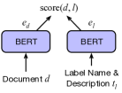
(a) Bi-Encoder

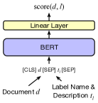
(b) Cross-Encoder

Figure 4. Two architectures that compute the similarity between a document $d$ and a candidate label $l$.

3.3.2. Metadata-Induced Contrastive Learning (MICoL)

Now we aim to fine-tune Bi-Encoder and Cross-Encoder to improve their re-ranking performance. (For Cross-Encoder, especially, we cannot even run it without fine-tuning because ${\bm{w}}$ needs to be learned.) If our task were fully supervised, we would have positive document–label training pairs $(d,l)$ indicating $d$ is labeled with $l$, and the training objective would be maximizing $score(d,l)$ for these positive pairs. However, we do not have any annotated documents with the zero-shot setting. In this case, to fine-tune above two architectures, we adopt a contrastive learning framework.

Instead of learning “what is what”, contrastive learning (Chen et al., 2020) tries to learn “what is similar to what”. In our problem setting, we assume there is a collection of document pairs $(d,d^{+})$, where $d$ and $d^{+}$ are similar to each other, e.g., $d^{+}$ is reachable from $d$ via a specified meta-path or meta-graph. For each $d$, we can also randomly sample a set of documents $\{d_{i}^{-}\}_{i=1}^{N}$ from the whole corpus $\mathcal{D}$. Contrastive learning aims to learn effective representations by pulling $d$ and $d^{+}$ together while pushing $d$ and $d_{i}^{-}$ apart. Taking Bi-Encoder as an example, we first use BERT to encode all documents.

(7) $${\bm{e}}_{d}={\rm BERT}(d),\ \ \ \ {\bm{e}}_{d^{+}}={\rm BERT}(d^{+}),\ \ \ \ {\bm{e}}_{d_{i}^{-}}={\rm BERT}(d_{i}^{-}).$$

Following Chen et al.’s seminal work (Chen et al., 2020), the contrastive loss can be defined as

(8) $$-\log\frac{\exp(\cos({\bm{e}}_{d},{\bm{e}}_{d^{+}})/\tau)}{\exp(\cos({\bm{e}}_{d},{\bm{e}}_{d^{+}})/\tau)+\sum_{i=1}^{N}\exp(\cos({\bm{e}}_{d},{\bm{e}}_{d_{i}^{-}})/\tau)},$$

where $\tau$ is a temperature hyperparameter.

Now the problem becomes how to define similar document–document pairs $(d,d^{+})$. In Chen et al.’s original paper (Chen et al., 2020), they focus on learning visual representations, so they take two random transformations (e.g., cropping, distortion, rotation) of the same image as positive pairs. A similar approach has been adopted in learning language representations (Wu et al., 2020; Luo et al., 2021; Giorgi et al., 2021; Yan et al., 2021), but transformation techniques become word insertion, deletion, substitution, reordering (Wei and Zou, 2019), and back translation (Xie et al., 2020).

Instead of using those purely text-based techniques, we propose a simple but novel approach based on document metadata. That is, given a meta-path or a meta-graph $\mathcal{M}$, we define $(d,d^{+})$ as a similar document–document pair if and only if $d^{+}$ is reachable from $d$ via $\mathcal{M}$ (i.e., $d^{+}\in\mathcal{N}_{\mathcal{M}}(d)$, Definition 2.4).

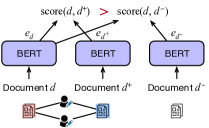
(a) Bi-Encoder fine-tuning

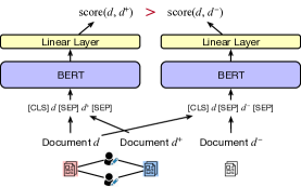
(b) Cross-Encoder fine-tuning

Figure 5. Metadata-induced contrastive learning to fine-tune Bi-Encoder and Cross-Encoder using $\mathcal{M}=P(AA)P$.

Formally, for Bi-Encoder, the metadata-induced contrastive loss is defined as

(9) $$\small\mathcal{J}_{\rm Bi}=\mathop{\mathbb{E}}_{\begin{subarray}{c}d^{+}\in\mathcal{N}_{\mathcal{M}}(d)\\ d_{i}^{-}\sim\mathcal{D}\end{subarray}}\bigg{[}-\log\frac{\exp(\cos({\bm{e}}_{d},{\bm{e}}_{d^{+}})/\tau)}{\exp(\cos({\bm{e}}_{d},{\bm{e}}_{d^{+}})/\tau)+\sum_{i=1}^{N}\exp(\cos({\bm{e}}_{d},{\bm{e}}_{d_{i}^{-}})/\tau)}\bigg{]}.$$

Similarly, for Cross-Encoder, we first compute $score(d,d^{+})$ and $score(d,d_{i}^{-})$.

(10) $$\begin{split}{\bm{e}}_{d||d^{+}}={\rm BERT}(d\ ||\ d^{+}),\ \ \ &\ \ \ \ {\bm{e}}_{d||d_{i}^{-}}={\rm BERT}(d\ ||\ d_{i}^{-}),\\ score(d,d^{+})={\bm{w}}^{\top}{\bm{e}}_{d||d^{+}},\ \ \ &\ \ \ \ score(d,d_{i}^{-})={\bm{w}}^{\top}{\bm{e}}_{d||d_{i}^{-}}.\end{split}$$

Then, the metadata-induced contrastive loss is

(11) $$\small\mathcal{J}_{\rm Cross}=\mathop{\mathbb{E}}_{\begin{subarray}{c}d^{+}\in\mathcal{N}_{\mathcal{M}}(d)\\ d_{i}^{-}\sim\mathcal{D}\end{subarray}}\bigg{[}-\log\frac{\exp(score(d,d^{+}))}{\exp(score(d,d^{+}))+\sum_{i=1}^{N}\exp(score(d,d_{i}^{-}))}\bigg{]}.$$

The BERT model is thus fine-tuned by minimizing the contrastive loss in Eq. (9) or (11). Figure 5 illustrates the fine-tuning process of both Bi-Encoder and Cross-Encoder using $\mathcal{M}=P(AA)P$.

Due to the space constraint, the training and inference procedures of the MICoL framework are formally summarized in Appendix A.2; the optimization details of MICoL (i.e., Eqs. (9) and (11)) are provided in Appendix A.3.

4. Experiments

4.1. Setup

Datasets. Given the task of metadata-aware LMTC, following (Zhang et al., 2021c), we perform evaluation on two large-scale datasets.

• MAG-CS (Wang et al., 2020b). The Microsoft Academic Graph (MAG) has a web-scale collection of scientific papers from various fields. In (Zhang et al., 2021c), 705,407 MAG papers published at 105 top CS conferences from 1990 to 2020 are selected to form a dataset with 15,808 labels.

• PubMed (Lu, 2011). PubMed has a web-scale collection of biomedical literature from MEDLINE, life science journals, and online books. In (Zhang et al., 2021c), 898,546 PubMed papers published in 150 top medicine journals from 2010 to 2020 are selected to form a dataset with 17,963 labels (i.e., MeSH terms (Coletti and Bleich, 2001)).

Under the fully supervised setting, Zhang et al. (Zhang et al., 2021c) split both datasets into training, validation, and testing sets. In this paper, we focus on the zero-shot setting. Therefore, we combine their training and validation sets together as our unlabeled input corpus $\mathcal{D}$ (that being said, we do not know the labels of these documents, and we only utilize their text and metadata information). We use their testing set as our testing documents $d\notin\mathcal{D}$. Dataset statistics are briefly listed in Table 1. More details are in Appendix A.4.

Table 1. Dataset statistics.

Dataset	#Training (Unlabeled)	#Testing	#Labels	Labels/Doc	Words/Doc
MAG-CS (Wang et al., 2020b)	634,874	70,533	15,808	5.59	126.55
PubMed (Lu, 2011)	808,692	89,854	17,963	7.80	199.14

Table 2. P@$k$ and NDCG@$k$ scores of compared algorithms on MAG-CS and PubMed. Bold: the highest score of zero-shot approaches. *: MICoL (Cross-Encoder, $P\rightarrow P\leftarrow P$) is significantly better than this algorithm with p-value $<0.05$. **: MICoL (Cross-Encoder, $P\rightarrow P\leftarrow P$) is significantly better than this algorithm with p-value $<0.01$.

	Algorithm	MAG-CS (Wang et al., 2020b)					PubMed (Lu, 2011)
		P@1	P@3	P@5	NDCG@3	NDCG@5	P@1	P@3	P@5	NDCG@3	NDCG@5
Zero-shot	Doc2Vec (Mikolov et al., 2013)	0.5697**	0.4613**	0.3814**	0.5043**	0.4719**	0.3888**	0.3283**	0.2859**	0.3463**	0.3252**
	SciBERT (Beltagy et al., 2019)	0.6440**	0.5030**	0.4011**	0.5545**	0.5061**	0.4427**	0.3572**	0.3031**	0.3809**	0.3510**
	ZeroShot-Entail (Yin et al., 2019)	0.6649**	0.5003**	0.3959**	0.5570**	0.5057**	0.5275**	0.4021	0.3299	0.4352	0.3913
	SPECTER (Cohan et al., 2020)	0.7107**	0.5381**	0.4184**	0.5979**	0.5365**	0.5286**	0.3923**	0.3181**	0.4273**	0.3815**
	EDA (Wei and Zou, 2019)	0.6442**	0.4939**	0.3948**	0.5471**	0.5000**	0.4919	0.3754*	0.3101*	0.4058*	0.3667*
	UDA (Xie et al., 2020)	0.6291**	0.4848**	0.3897**	0.5362**	0.4918**	0.4795**	0.3696**	0.3067**	0.3986**	0.3614**
	MICoL (Bi-Encoder, $P\rightarrow P\leftarrow P$)	0.7062*	0.5369*	0.4184*	0.5960*	0.5355*	0.5124**	0.3869*	0.3172*	0.4196*	0.3774*
	MICoL (Bi-Encoder, $P\leftarrow(PP)\rightarrow P$)	0.7050*	0.5344*	0.4161*	0.5937*	0.5331*	0.5198**	0.3876*	0.3172*	0.4215*	0.3786*
	MICoL (Cross-Encoder, $P\rightarrow P\leftarrow P$)	0.7177	0.5444	0.4219	0.6048	0.5415	0.5412	0.4036	0.3257	0.4391	0.3906
	MICoL (Cross-Encoder, $P\leftarrow(PP)\rightarrow P$)	0.7061	0.5376	0.4187	0.5964	0.5357	0.5218	0.3911	0.3172*	0.4249	0.3794
Supervised	MATCH (Zhang et al., 2021c) (10K Training)	0.4423**	0.2851**	0.2152**	0.3375**	0.3003**	0.6915	0.3869*	0.2785**	0.4649	0.3896
	MATCH (Zhang et al., 2021c) (50K Training)	0.6215**	0.4280**	0.3269**	0.4987**	0.4489**	0.7701	0.4716	0.3585	0.5497	0.4750
	MATCH (Zhang et al., 2021c) (100K Training)	0.8321	0.6520	0.5142	0.7342	0.6761	0.8286	0.5680	0.4410	0.6405	0.5626
	MATCH (Zhang et al., 2021c) (Full, 560K+ Training)	0.9114	0.7634	0.6312	0.8486	0.8076	0.9151	0.7425	0.6104	0.8001	0.7310

Compared Methods. We evaluate MICoL against a variety of baseline methods using text embedding, pre-trained language models, and text-based contrastive learning. Since the major technical contribution of MICoL is in the re-ranking stage, all the baselines below are used as re-rankers after the same retrieval stage proposed in Section 3.2.

• Doc2Vec (Le and Mikolov, 2014) is a text embedding method. We use it to embed documents and labels into a shared semantic space according to their text information. Then, for each document, we rank all candidate labels according to their cosine similarity with the document in the embedding space.

• SciBERT (Beltagy et al., 2019) is a BERT-based language model pre-trained on a large set of computer science and biomedical papers. Taking it as a baseline, we do not perform fine-tuning, so it can only be used in Bi-Encoder. (In Cross-Encoder, the linear layer is not pre-trained, thus cannot be used without fine-tuning.)

• ZeroShot-Entail (Yin et al., 2019) is a pre-trained language model for zero-shot text classification. It is a textual entailment model that predicts to what extent a document (as the premise) can entail the template “this document is about {label_name}” (as the hypothesis). To make this method more competitive, we change its internal BERT-base-uncased model to RoBERTa-large-mnli.

• SPECTER (Cohan et al., 2020) is a pre-trained language model for scientific documents that leverages paper citation information. It is built upon SciBERT and takes citation prediction as the pre-training objective. We use it in the Bi-Encoder architecture without fine-tuning.

• EDA (Wei and Zou, 2019) is a text data augmentation method. Given a document, it proposes four simple operations – synonym replacement, random insertion, random swap, and random deletion – to create a new artificial document. We view the original document and the new one as a positive document–document pair and use all these pairs to perform contrastive learning to fine-tune SciBERT.

• UDA (Xie et al., 2020) is another text data augmentation method. It performs back translation and TF-IDF word replacement to generate new documents that are similar to the original one. We use these pairs to perform contrastive learning to fine-tune SciBERT. Both EDA and UDA can be leveraged to fine-tune a Bi-Encoder or a Cross-Encoder, and we report the higher performance between the two architectures.

• MICoL is our proposed framework. We study the performance of 10 meta-paths/meta-graphs $\{P\rightarrow P,P\leftarrow P,PAP,PVP,P\rightarrow P\leftarrow P,P\leftarrow P\rightarrow P,P(AA)P,P(AV)P,P\rightarrow(PP)\leftarrow P,P\leftarrow(PP)\rightarrow P\}$ when fine-tuning Bi-Encoder and Cross-Encoder. We choose SciBERT as our base model to be fine-tuned.

We also report the performance of a fully supervised method for reference.

• MATCH (Zhang et al., 2021c) is the state-of-the-art supervised approach for metadata-aware multi-label text classification. Because we do not consider label hierarchy in our problem setting, we report the performance of MATCH-NoHierarchy with various sizes of training data for comparison.

Evaluation Metrics. Following the commonly used evaluation on multi-label text classification (Liu et al., 2017; You et al., 2019; Zhang et al., 2021c), we adopt two rank-based metrics: P@$k$ and NDCG@$k$, where $k=1,3,5$. For a document $d$, let ${\bm{y}}_{d}\in\{0,1\}^{|\mathcal{L}|}$ be its ground truth label vector and ${\rm rank}(i)$ be the index of the $i$-th highest predicted label according to the re-ranker.

$$\small\begin{split}{\rm P@}k&=\frac{1}{k}\sum_{i=1}^{k}y_{d,{\rm rank}(i)}.\\ {\rm DCG@}k=\sum_{i=1}^{k}\frac{y_{d,{\rm rank}(i)}}{\log(i+1)},\ \ \ &{\rm NDCG@}k=\frac{{\rm DCG@}k}{\sum_{i=1}^{\min(k,||{\bm{y}}_{d}||_{0})}\frac{1}{\log(i+1)}}.\end{split}$$

Table 3. PSP@$k$ and PSN@$k$ scores of compared algorithms on MAG-CS and PubMed. Bold, *, and **: the same meaning as in Table 2. We also show the ratio $\rm PSP@1/P@1$. The higher ${\rm PSP@}k/{\rm P@}k$ is, the more infrequent the correctly predicted labels are.

	Algorithm	MAG-CS (Wang et al., 2020b)						PubMed (Lu, 2011)
		PSP@1	PSP@3	PSP@5	PSN@3	PSN@5	$\frac{\rm PSP@1}{\rm P@1}$	PSP@1	PSP@3	PSP@5	PSN@3	PSN@5	$\frac{\rm PSP@1}{\rm P@1}$
Zero-shot	Doc2Vec (Mikolov et al., 2013)	0.4287**	0.4623**	0.4656**	0.4450**	0.4425**	0.75	0.2717**	0.2948**	0.3029**	0.2856**	0.2879**	0.70
	SciBERT (Beltagy et al., 2019)	0.4668**	0.4958**	0.4843**	0.4788**	0.4667**	0.72	0.3149**	0.3231**	0.3221**	0.3174**	0.3131**	0.71
	ZeroShot-Entail (Yin et al., 2019)	0.4796**	0.4892**	0.4759**	0.4777**	0.4644**	0.72	0.3617**	0.3498**	0.3389**	0.3492**	0.3378**	0.69
	SPECTER (Cohan et al., 2020)	0.5304	0.5334*	0.5059*	0.5223	0.4988*	0.75	0.3907**	0.3638**	0.3442**	0.3666**	0.3489**	0.74
	EDA (Wei and Zou, 2019)	0.4916**	0.4968**	0.4821**	0.4859**	0.4708**	0.76	0.3572*	0.3451*	0.3334*	0.3442*	0.3322*	0.73
	UDA (Xie et al., 2020)	0.4850**	0.4907**	0.4771**	0.4797**	0.4654**	0.77	0.3547**	0.3423**	0.3311**	0.3416**	0.3298**	0.74
	MICoL (Bi-Encoder, $P\rightarrow P\leftarrow P$)	0.5176	0.5311	0.5065	0.5175	0.4963	0.73	0.3676**	0.3559**	0.3423*	0.3550**	0.3418**	0.72
	MICoL (Bi-Encoder, $P\leftarrow(PP)\rightarrow P$)	0.5160	0.5281	0.5037	0.5150	0.4940	0.73	0.3780**	0.3589*	0.3423*	0.3597**	0.3450**	0.73
	MICoL (Cross-Encoder, $P\rightarrow P\leftarrow P$)	0.5375	0.5415	0.5118	0.5302	0.5052	0.75	0.4105	0.3807	0.3558	0.3841	0.3625	0.76
	MICoL (Cross-Encoder, $P\leftarrow(PP)\rightarrow P$)	0.5326	0.5363	0.5087	0.5249	0.5013	0.75	0.3871	0.3664	0.3462	0.3677	0.3496	0.74
Supervised	MATCH (Zhang et al., 2021c) (10K Training)	0.1978**	0.1807**	0.1712**	0.1850**	0.1764**	0.45	0.2840**	0.2138**	0.1870**	0.2332**	0.2139**	0.41
	MATCH (Zhang et al., 2021c) (50K Training)	0.2854**	0.2830**	0.2738**	0.2838**	0.2780**	0.46	0.3201**	0.2715**	0.2532**	0.2848**	0.2713**	0.42
	MATCH (Zhang et al., 2021c) (100K Training)	0.4271**	0.4750**	0.4737*	0.4624**	0.4635**	0.51	0.3576**	0.3579**	0.3456*	0.3584**	0.3507**	0.43
	MATCH (Zhang et al., 2021c) (200K Training)	0.4695**	0.5401	0.5530	0.5217	0.5325	0.54	0.3732**	0.3988	0.3905	0.3913	0.3882	0.44
	MATCH (Zhang et al., 2021c) (Full, 560K+ Training)	0.5501	0.6397	0.6627	0.6171	0.6345	0.60	0.4371	0.5188	0.5200	0.4978	0.5011	0.48

4.2. Performance Comparison

Table 2 shows P@$k$ and NDCG@$k$ scores of compared algorithms on MAG-CS and PubMed. We run each experiment three times with the average score reported. (SciBERT, Zero-Shot-Entail, and SPECTER are deterministic according to our usage, so we run them only once.) To show statistical significance, we conduct two-tailed unpaired t-tests to compare the best performed MICoL model and other approaches including MATCH. (When comparing MICoL with three deterministic approaches, we conduct two-tailed Z-tests instead.) The significance level of each result is marked in Table 2. For MICoL, we show the performance of one meta-path $P\rightarrow P\leftarrow P$ and one meta-graph $P\leftarrow(PP)\rightarrow P$ here. The performance of other meta-paths/meta-graphs will be presented in Table 4 and discussed in Section 4.4.

From Table 2, we observe that: (1) MICoL (Cross-Encoder, $P\rightarrow P\leftarrow P$) significantly outperforms all zero-shot baselines in most cases, except that it is slightly worse than ZeroShot-Entail on PubMed in terms of P@5 and NDCG@5. (2) On MAG-CS, MICoL (Cross-Encoder, $P\rightarrow P\leftarrow P$) performs significantly better than the supervised MATCH model with 50K labeled training data. On PubMed, MICoL can be competitive with MATCH trained on more than 10K annotated documents in terms of P@3, P@5, and NDCG@5. (3) Using purely text-based augmentation approaches (i.e., EDA and UDA) to perform contrastive learning is not consistently beneficial. In fact, EDA and UDA perform even worse than unfine-tuned SciBERT on MAG-CS. In contrast, our proposed metadata-induced contrastive learning consistently boosts the performance of SciBERT, and the improvements are much more significant than those of text-based contrastive learning. (4) For both $P\rightarrow P\leftarrow P$ and $P\leftarrow(PP)\rightarrow P$, Cross-Encoder performs better than Bi-Encoder within the MICoL framework. In Section 4.4, we will show that this observation is generalizable to most meta-paths and meta-graphs we use.

4.3. Performance on Tail Labels

Tail labels refer to those labels relevant to only a few documents in the dataset. They are usually more fine-grained and informative than head labels (i.e., frequent ones). However, predicting tail labels is less “rewarding” for models to achieve high P@$k$ and NDCG@$k$ scores. Therefore, new scoring functions are designed to promote infrequent label prediction by giving the model a higher “reward” when it predicts a tail label correctly. Propensity-scored P@$k$ (PSP@$k$) and propensity-scored NDCG@$k$ (PSNDCG@$k$, abbreviated to PSN@$k$ in this paper) are thus proposed in (Jain et al., 2016) and widely used in LMTC evaluation (You et al., 2019; Saini et al., 2021; Mittal et al., 2021; Wei et al., 2021; Gupta et al., 2021). PSP@$k$ and PSN@$k$ are defined as follows.

$$\small\begin{split}\frac{1}{p_{l}}=1+C(N_{l}+B)^{-A},\ \ \ {\rm PSP}&{@}k=\frac{1}{k}\sum_{i=1}^{k}\frac{y_{d,{\rm rank}(i)}}{p_{d,{\rm rank}(i)}}.\\ {\rm PSDCG@}k=\sum_{i=1}^{k}\frac{y_{d,{\rm rank}(i)}}{p_{d,{\rm rank}(i)}\log(i+1)},\ \ \ &{\rm PSN@}k=\frac{{\rm PSDCG@}k}{\sum_{i=1}^{\min(k,||{\bm{y}}_{d}||_{0})}\frac{1}{\log(i+1)}}.\end{split}$$

Here, $\frac{1}{p_{l}}$ is the “reward” of predicting the label $l$ correctly; $N_{l}$ is the number of documents relevant to $l$ in the training set. Following previously established parameter values (Jain et al., 2016; You et al., 2019; Wei et al., 2021), we set $A=0.55$, $B=1.5$, and $C=(\log|\mathcal{D}|-1)(B+1)^{A}$. Therefore, the less frequent a label is, the higher reward one can get by predicting it correctly. Table 3 shows the PSP@$k$ and PSN@$k$ scores of compared methods.

As shown in Table 3, when we use PSP@$k$ and PSN@$k$ as evaluation metrics, MICoL becomes more powerful. MICoL (Cross-Encoder, $P\rightarrow P\leftarrow P$) significantly outperforms all zero-shot baselines, and it is on par with MATCH trained on 100K–200K labeled documents. According to the definition of PSP@$k$ and P@$k$, the ratio ${\rm PSP@}k/{\rm P@}k$ reflects the average “reward” a model gets from its correctly predicted labels. The higher ${\rm PSP@}k/{\rm P@}k$ is, the more infrequent the correctly predicted labels are. We show $\rm PSP@1/P@1$ in Table 3. We observe that labels predicted by MICoL (and all other zero-shot methods) are much more infrequent than labels predicted by the supervised MATCH model. The reason could be that zero-shot methods cannot see any labeled data during training, thus they get no hints of frequent labels and are not biased towards head labels. This helps alleviate the deteriorated performance of supervised models on long-tailed labels as observed in (Wei and Li, 2018; Wei et al., 2021).

4.4. Effect of Meta-Path and Meta-Graph

Table 4. P@$k$ and NDCG@$k$ scores of MICoL using different meta-paths/meta-graphs. Bold: the best model. *: significantly worse than the best model with p-value $<0.05$. **: significantly worse than the best model with p-value $<0.01$. All meta-paths and meta-graphs, except $PVP$, can improve the classification performance upon unfine-tuned SciBERT.

Algorithm	MAG-CS (Wang et al., 2020b)					PubMed (Lu, 2011)
	P@1	P@3	P@5	NDCG@3	NDCG@5	P@1	P@3	P@5	NDCG@3	NDCG@5
Unfine-tuned SciBERT	0.6599**	0.5117**	0.4056**	0.5651**	0.5136**	0.4371**	0.3544**	0.3014**	0.3775**	0.3485**
MICoL (Bi-Encoder, $PAP$)	0.6877**	0.5285**	0.4143**	0.5852**	0.5280**	0.4974**	0.3818**	0.3154*	0.4122**	0.3727**
MICoL (Bi-Encoder, $PVP$)	0.6589**	0.5123**	0.4063**	0.5656**	0.5145**	0.4440**	0.3507**	0.2966**	0.3761**	0.3458**
MICoL (Bi-Encoder, $P\rightarrow P$)	0.7094	0.5391	0.4190	0.5982	0.5367	0.5200*	0.3903*	0.3195	0.4240*	0.3808*
MICoL (Bi-Encoder, $P\leftarrow P$)	0.7095*	0.5374*	0.4178*	0.5970*	0.5356*	0.5195**	0.3905*	0.3192	0.4240*	0.3806*
MICoL (Bi-Encoder, $P\rightarrow P\leftarrow P$)	0.7062*	0.5369*	0.4184*	0.5960*	0.5355*	0.5124**	0.3869*	0.3172*	0.4196*	0.3774*
MICoL (Bi-Encoder, $P\leftarrow P\rightarrow P$)	0.7039*	0.5379*	0.4187*	0.5963*	0.5356*	0.5174**	0.3886*	0.3187*	0.4220*	0.3795*
MICoL (Bi-Encoder, $P(AA)P$)	0.6873**	0.5272**	0.4130**	0.5840**	0.5269**	0.4963**	0.3794**	0.3139**	0.4101**	0.3711**
MICoL (Bi-Encoder, $P(AV)P$)	0.6832**	0.5263**	0.4135**	0.5823**	0.5263**	0.4894**	0.3743**	0.3099**	0.4045**	0.3664**
MICoL (Bi-Encoder, $P\rightarrow(PP)\leftarrow P$)	0.7015**	0.5334**	0.4160**	0.5920**	0.5322**	0.5163**	0.3879*	0.3172*	0.4211*	0.3781*
MICoL (Bi-Encoder, $P\leftarrow(PP)\rightarrow P$)	0.7050*	0.5344*	0.4161*	0.5937*	0.5331*	0.5198**	0.3876*	0.3172*	0.4215*	0.3786*
MICoL (Cross-Encoder, $PAP$)	0.7034*	0.5355	0.4168	0.5943	0.5337	0.5212**	0.3921*	0.3207	0.4255*	0.3818*
MICoL (Cross-Encoder, $PVP$)	0.6720*	0.5203*	0.4103*	0.5750*	0.5210*	0.4668**	0.3633**	0.3051**	0.3908**	0.3574**
MICoL (Cross-Encoder, $P\rightarrow P$)	0.7033*	0.5391	0.4201	0.5971*	0.5365*	0.5266	0.3946	0.3207	0.4286	0.3830
MICoL (Cross-Encoder, $P\leftarrow P$)	0.7169	0.5430	0.4214	0.6033	0.5406	0.5265	0.3924	0.3186	0.4268	0.3811
MICoL (Cross-Encoder, $P\rightarrow P\leftarrow P$)	0.7177	0.5444	0.4219	0.6048	0.5415	0.5412	0.4036	0.3257	0.4391	0.3906
MICoL (Cross-Encoder, $P\leftarrow P\rightarrow P$)	0.7045	0.5356*	0.4168*	0.5944*	0.5336*	0.5243*	0.3932*	0.3190*	0.4271*	0.3814*
MICoL (Cross-Encoder, $P(AA)P$)	0.7028	0.5351	0.4171	0.5939	0.5338	0.5290*	0.3937	0.3201	0.4285*	0.3830
MICoL (Cross-Encoder, $P(AV)P$)	0.7024*	0.5354*	0.4177	0.5940*	0.5343*	0.5164**	0.3897*	0.3195*	0.4225*	0.3797*
MICoL (Cross-Encoder, $P\rightarrow(PP)\leftarrow P$)	0.7076*	0.5379*	0.4188	0.5971*	0.5363*	0.5186	0.3924*	0.3184*	0.4254*	0.3800*
MICoL (Cross-Encoder, $P\leftarrow(PP)\rightarrow P$)	0.7061	0.5376	0.4187	0.5964	0.5357	0.5218	0.3911	0.3172*	0.4249	0.3794

Table 4 shows the performance of all 20 MICoL variants (2 architectures $\times$ 10 meta-paths/meta-graphs). We have the following observations: (1) All meta-paths and meta-graphs used in MICoL, except $PVP$, can improve the classification performance upon unfine-tuned SciBERT. For $PVP$, the unsatisfying performance is expected because venue information alone (e.g., ACL) is too weak to distinguish between fine-grained labels (e.g., “Named Entity Recognition” and “Entity Linking”). In Appendix A.1, we provide a mathematical interpretation of why some meta-paths/meta-graphs (e.g., $PVP$ or $P(AAAAA)P$) may not perform well within our MICoL framework. In short, the results in Table 4 demonstrate the effectiveness of MICoL across different meta-paths/meta-graphs. (2) Cross-Encoder models perform better than their Bi-Encoder counterparts in most cases (8 out of 10 meta-paths/meta-graphs on MAG-CS and 10 out of 10 on PubMed, in terms of P@1). (3) In contrast to the gap between Bi-Encoder and Cross-Encoder, the difference among citation-based meta-paths and meta-graphs is less significant. It would be an interesting future work to automatically select the most effective meta-paths/meta-graphs, although related studies on heterogeneous network representation learning (Dong et al., 2017; Wang et al., 2019a; Yang et al., 2020) often require users to specify them.

5. Related Work

Zero-Shot Multi-Label Text Classification. Yin et al. (Yin et al., 2019) divide existing studies on zero-shot text classification into two settings: the restrictive setting (Wang et al., 2019b) assumes training documents are given for some seen classes and the trained classifier should be able to predict unseen classes; the wild setting does not assume any seen classes and the classifier needs to make prediction without any annotated training data. Most previous studies on zero-shot LMTC (Chalkidis et al., 2019; Nam et al., 2015, 2016; Rios and Kavuluru, 2018; Gupta et al., 2021) focus on the restrictive setting, while this paper studies the more challenging wild setting. Under the wild setting, a pioneering approach is dataless classification (Chang et al., 2008; Song and Roth, 2014) which maps documents and labels into the same space of Wikipedia concepts. Recent studies further leverage convolutional networks (Meng et al., 2018) or pre-trained language models (Mekala and Shang, 2020; Meng et al., 2020; Wang et al., 2020a). While these models rely on label names only, they all assume that each document belongs to one category, thus are not applicable to the multi-label setting. Yin et al. (Yin et al., 2019) propose to treat zero-shot text classification as a textual entailment problem and leverage pre-trained language models to solve it; Shen et al. (Shen et al., 2021) further extend the idea to hierarchical zero-shot text classification. Compared with their studies, we utilize document metadata as complementary signals to the text.

Metadata-Aware Text Classification. In some specific classification tasks, document metadata have been used as label indicators (e.g., reviewer and product information in review sentiment analysis (Tang et al., 2015), user profile information in tweet localization (Schulz et al., 2013; Zhang et al., 2017)). Kim et al. (Kim et al., 2019) propose a generic approach to add categorical metadata into neural text classifiers. Zhang et al. (Zhang et al., 2021c) further study metadata-aware LMTC. However, all these studies focus on the fully supervised setting. Some studies (Zhang et al., 2020, 2021a, 2021d, 2021b) leverage metadata in few-shot text classification. Nevertheless, in LMTC, since the label space is large, it becomes prohibitive to provide even a few training samples for each label. Mekala et al. (Mekala et al., 2020) consider metadata in zero-shot single-label text classification given a small label space, but their approach can hardly be generalized to LMTC.

Text Contrastive Learning. Recently, contrastive learning has become a promising trend in unsupervised text representation learning. The general idea is to use various data augmentation techniques (Wei and Zou, 2019; Xie et al., 2020; Feng et al., 2021) to generate similar text pairs and find a mapping function to make them closer in the representation space while pushing away dissimilar ones. Therefore, the major novelty of those studies is often the data augmentation techniques they propose. For example, DeCLUTR (Giorgi et al., 2021) samples two text spans from the same document; CLEAR (Wu et al., 2020) adopts span deletion, span reordering, and synonym substitution; DECA (Luo et al., 2021) uses synonym substitution, antonym augmentation, and back translation; SimCSE (Gao et al., 2021b) applies two different hidden dropout masks when encoding the same sentence; ConSERT (Yan et al., 2021) employs token reordering, deletion, dropout, and adversarial attack. However, all these data augmentation approaches manipulate text information only to generate artificial sentences/documents, while our MICoL exploits metadata information to find real documents that are similar to each other.

6. Conclusions and Future Work

In this paper, we study zero-shot multi-label text classification with document metadata as complementary signals, which avail us with heterogeneous network information besides corpus. Our setting does not require any annotated training documents with labels and only relies on label names and descriptions. We propose a novel metadata-induced contrastive learning (MICoL) method to train a BERT-based document–label relevance scorer. We study two types of architectures (i.e., Bi-Encoder and Cross-Encoder) and 10 different meta-paths/meta-graphs within the MICoL framework. MICoL achieves strong performance on two large datasets, outperforming competitive baselines under the zero-shot setting and being on par with the supervised MATCH model trained on 10K–200K labeled documents. In the future, it is of interest to extend MICoL to zero-shot hierarchical text classification and explore whether label hierarchy could provide additional signals to contrastive learning.

Appendix A Supplementary Material

A.1. Interpretation of MICoL

We have proposed the MICoL objective (i.e., Eq. (9) or (11)) to fine-tune BERT. Here, we provide the interpretation of this objective function by answering the following two questions.

• Q1. MICoL does not require any labeled data during fine-tuning. What is the relationship between MICoL and supervised fine-tuning approaches?

• Q2. Under what conditions will the MICoL objective be closer to the supervised objective (thus MICoL may perform better in classification)?

To answer these two questions, let us first consider how supervised approaches fine-tune BERT in multi-label text classification. Assume each document $d\in\mathcal{D}$ is annotated with its relevant labels $\mathcal{L}_{d}$. We can sample a positive label $l^{+}$ from $\mathcal{L}_{d}$ and several negative labels $\{l_{i}^{-}\}_{i=1}^{N}$ from $\mathcal{L}$. The supervised learning process learns effective representations by pulling $d$ and $l^{+}$ together while pushing $d$ and $l_{i}^{-}$ apart. Using either Bi-Encoder (Eqs. (3) and (4)) or Cross-Encoder (Eqs. (5) and (6)), the learning objective can be defined as

(12) $$\small\mathcal{J}_{\rm Sup}=\mathop{\mathbb{E}}_{\begin{subarray}{c}l^{+}\in\mathcal{L}_{d}\\ l_{i}^{-}\sim\mathcal{L}\end{subarray}}\bigg{[}-\log\frac{\exp(score(d,l^{+}))}{\exp(score(d,l^{+}))+\sum_{i=1}^{N}\exp(score(d,l_{i}^{-}))}\bigg{]}.$$

If we view each label $l$’s text information (i.e., label name and description) as a “document”, it is natural to assume this “document” $t_{l}$ is relevant to the label $l$. For example, in Figure 1, the description of “Webgraph” can be viewed as a “document” specifically relevant to “Webgraph” itself. Therefore, if we follow the notation of $\mathcal{L}_{d}$ and use $\mathcal{L}_{l}$ to denote the set of labels relevant to $t_{l}$, it is equivalent to have $\mathcal{L}_{l}=\{l\}$. In this case, we have $l\in\mathcal{L}_{d}$ if and only if $\mathcal{L}_{d}\cap\mathcal{L}_{l}\neq\emptyset$. Then, the supervised loss in Eq. (12) is equivalent to

(13) $$\small\mathcal{J}_{\rm Sup}=\mathop{\mathbb{E}}_{\begin{subarray}{c}\mathcal{L}_{d}\cap\mathcal{L}_{l^{+}}\neq\emptyset\\ l_{i}^{-}\sim\mathcal{L}\end{subarray}}\bigg{[}-\log\frac{\exp(score(d,l^{+}))}{\exp(score(d,l^{+}))+\sum_{i=1}^{N}\exp(score(d,l_{i}^{-}))}\bigg{]}.$$

If we replace $l^{+}$ and $l_{i}^{-}$ in Eq. (13) with $d^{+}$ and $d_{i}^{-}$, respectively, (in other words, if we replace label text information with real documents), the supervised loss can be rewritten into the following form.

(14) $$\small\mathcal{J}^{\prime}_{\rm Sup}=\mathop{\mathbb{E}}_{\begin{subarray}{c}\mathcal{L}_{d}\cap\mathcal{L}_{d^{+}}\neq\emptyset\\ d_{i}^{-}\sim\mathcal{D}\end{subarray}}\bigg{[}-\log\frac{\exp(score(d,d^{+}))}{\exp(score(d,d^{+}))+\sum_{i=1}^{N}\exp(score(d,d_{i}^{-}))}\bigg{]}.$$

By comparing Eq. (14) with Eq. (9) (when $\tau=1$) and Eq. (11), we can answer Q1: MICoL and supervised loss share the same functional format, and the only difference is the distribution of training data $(d,d^{+})$ pairs. For supervised loss, annotated documents are available, so positive document–document pairs $(d,d^{+})$ can be derived using their labels; for MICoL, there are no annotated training samples, positive document–document pairs $(d,d^{+})$ are derived from metadata instead.

Now we proceed to Q2. Given the answer of Q1, the key difference between $\mathcal{J}_{\rm Bi}$ (or $\mathcal{J}_{\rm Cross}$) and $\mathcal{J}^{\prime}_{\rm Sup}$ is how we sample the positive partner $d^{+}$ for each document $d$. Let us explicitly write down the two distributions for sampling $d^{+}$. For MICoL, the distribution is

(15) $${\rm P}_{\textsc{MICoL}}(d^{+}|d)=\begin{cases}1/X,&d^{+}\in\mathcal{N}_{\mathcal{M}}(d);\\ 0,&d^{+}\notin\mathcal{N}_{\mathcal{M}}(d).\end{cases}$$

Here, $X=|\mathcal{N}_{\mathcal{M}}(d)|$.

For the supervised loss in Eq. (14), the distribution is

(16) $${\rm P}_{\rm Sup}(d^{+}|d)=\begin{cases}1/Y,&\mathcal{L}_{d}\cap\mathcal{L}_{d^{+}}\neq\emptyset;\\ 0,&\mathcal{L}_{d}\cap\mathcal{L}_{d^{+}}=\emptyset.\end{cases}$$

Here, $Y=|\{d^{+}|\mathcal{L}_{d}\cap\mathcal{L}_{d^{+}}\neq\emptyset\}|$.

It is straightforward to compute the Jensen-Shannon (JS) divergence between ${\rm P}_{\textsc{MICoL}}$ and ${\rm P}_{\rm Sup}$.

(17) $$\begin{split}JS({\rm P}_{\textsc{MICoL}}||{\rm P}_{\rm Sup})=&\frac{1}{2}\log\frac{2X}{X+Y}+\frac{1}{2}\sum_{\begin{subarray}{c}d^{+}\in\mathcal{N}_{\mathcal{M}}(d)\\ \mathcal{L}_{d}\cap\mathcal{L}_{d^{+}}=\emptyset\end{subarray}}\frac{1}{X}\log\Big{(}1+\frac{X}{Y}\Big{)}\ +\\ &\frac{1}{2}\log\frac{2Y}{X+Y}+\frac{1}{2}\sum_{\begin{subarray}{c}\mathcal{L}_{d}\cap\mathcal{L}_{d^{+}}\neq\emptyset\\ d^{+}\notin\mathcal{N}_{\mathcal{M}}(d)\end{subarray}}\frac{1}{Y}\log\Big{(}1+\frac{Y}{X}\Big{)}.\end{split}$$

When $JS({\rm P}_{\textsc{MICoL}}||{\rm P}_{\rm Sup})$ is small, ${\rm P}_{\textsc{MICoL}}$ is close to ${\rm P}_{\rm Sup}$, thus the MICoL objective $\mathcal{J}_{\rm Bi}$ or $\mathcal{J}_{\rm Cross}$ is similar to the supervised objective $\mathcal{J}^{\prime}_{\rm Sup}$. To make $JS({\rm P}_{\textsc{MICoL}}||{\rm P}_{\rm Sup})$ smaller, the meta-path/meta-graph $\mathcal{M}$ should satisfy the following two properties as close as possible:

Property 1: $d^{+}\in\mathcal{N}_{\mathcal{M}}(d)\Rightarrow\mathcal{L}_{d}\cap\mathcal{L}_{d^{+}}\neq\emptyset$. Intuitively, this property means that if $d^{+}$ is reachable from $d$ via $\mathcal{M}$, then $d$ and $d^{+}$ should have similar topic labels. When this property is perfectly satisfied, the second term in Eq. (17) is 0.

Property 2 (the inverse of Property 1): $\mathcal{L}_{d}\cap\mathcal{L}_{d^{+}}\neq\emptyset\Rightarrow d^{+}\in\mathcal{N}_{\mathcal{M}}(d)$. This property implies that if $d$ and $d^{+}$ have similar labels, then $d^{+}$ should be reachable from $d$ via $\mathcal{M}$. When this property is perfectly satisfied, the fourth term in Eq. (17) is 0.

For example, when the label space is fine-grained, using $\mathcal{M}=PVP$ may not be a good choice because sharing the same venue is not sufficient to conclude that two papers have similar fine-grained labels. $PVP$ actually violates Property 1 in this case. On the other hand, when the label space is coarse-grained, using $\mathcal{M}=P(AAAAA)P$ may not be suitable because two papers in the same category do not necessarily have so many common authors. In this case, $P(AAAAA)P$ violates Property 2.

A.2. Training and Inference Procedures of MICoL

Input: An unlabeled corpus $\mathcal{D}$ with metadata $G=(\mathcal{V},\mathcal{E})$;

             a meta-path/meta-graph $\mathcal{M}$;

             the pre-trained BERT model.

Output: A fine-tuned BERT model.

1 Sample $d$, $d^{+}$, and $\{d_{i}^{-}\}_{i=1}^{N}$ from $\mathcal{D}$ according to $\mathcal{M}$;

2 if using Bi-Encoder for fine-tuning then

3       ${\bm{e}}_{d}$, ${\bm{e}}_{d^{+}}$, $\{{\bm{e}}_{d_{i}^{-}}\}_{i=1}^{N}\leftarrow$ Eq. (7);

4       Fine-tuning BERT by optimizing Eq. (9);

5      

6else if using Cross-Encoder for fine-tuning then

7       $score(d,d^{+})$, $score(d,d_{i}^{-})\leftarrow$ Eq. (10);

8       Fine-tuning BERT by optimizing Eq. (11);

9      

10 Return the fine-tuned BERT;

Algorithm 1 MICoL Training

Input: A label space $\mathcal{L}$ with label names and descriptions $t_{l}$;

             the fine-tuned BERT model;

             a new document $d\notin\mathcal{D}$.

Output: $d$’s relevant labels $\mathcal{L}_{d}\subseteq\mathcal{L}$.

1 // The Retrieval Stage;

2 $\mathcal{C}_{\rm exact}(d)\leftarrow$ exact label name matching;

3 $\mathcal{C}_{\rm BM25}(d)\leftarrow$ Eq. (2);

4 $\mathcal{C}(d)=\mathcal{C}_{\rm exact}(d)\cup\mathcal{C}_{\rm BM25}(d)$;

5 // The Re-ranking Stage;

6 for $l\in\mathcal{C}(d)$ do

7       if using Bi-Encoder then

8             ${\bm{e}}_{d}$, ${\bm{e}}_{l}\leftarrow$ Eq. (3) using the fine-tuned BERT model;

9             $score(d,l)\leftarrow$ Eq. (4);

10            

11      else if using Cross-Encoder then

12             ${\bm{e}}_{d||t_{l}}\leftarrow$ Eq. (5) using the fine-tuned BERT model;

13             $score(d,l)\leftarrow$ Eq. (6);

14            

15      

16Rank $l\in\mathcal{C}(d)$ according to $score(d,l)$;

17 Return $\mathcal{L}_{d}=\{$top-$k$ ranked labels in $\mathcal{C}(d)\}$;

Algorithm 2 MICoL Inference

We summarize the complete training and inference procedures in Algorithms 1 and 2, respectively. The goal of training is to obtain a fine-tuned BERT model, which is later used in the re-ranking stage of inference. Note that during the model training phase, we calculate the similarity score between two documents, while during the inference phase, we calculate the score between a document and a label (represented by its name and description).

A.3. Implementation

A.3.1. Optimization of MICoL

To approximate the expectation in Eqs. (9) and (11) during optimization, we adopt a sampling strategy. Specifically, we first sample a set of documents from $\mathcal{D}$. For each sampled document $d$, we pick one $d^{+}$ from $\mathcal{N}_{\mathcal{M}}(d)$ as $d$’s positive partner (if $\mathcal{N}_{\mathcal{M}}(d)\neq\emptyset$). When fine-tuning the Bi-Encoder, following (Chen et al., 2020), $d$’s negative partners $\{d_{i}^{-}\}_{i=1}^{N}$ are the positive partner of other documents in the same training batch. Each $d$ has 1 positive partner and $(\beta-1)$ negative partners, where $\beta$ is the batch size. Therefore, within each batch, to calculate Eq. (9), we need to call BERT $2\beta$ times (i.e., computing ${\bm{e}}_{d}$ and ${\bm{e}}_{d^{+}}$ for each $d$). When fine-tuning the Cross-Encoder, however, we would call BERT $\beta^{2}$ times within each batch if we used the same approach to obtain negative partners. To make the optimization process more efficient, for each $d$, we directly sample one negative partner $d^{-}$ from $\mathcal{D}$. Each $d$ has 1 positive partner and 1 negative partner. In this way, we only need to call BERT $2\beta$ times within each batch (i.e., encoding $(d\ ||\ d^{+})$ and $(d\ ||\ d^{-})$ for each $d$).

A.3.2. Parameter Settings of MICoL

For both Bi-Encoder and Cross-Encoder, we sample 50,000 $(d,d^{+})$ pairs for training and 5,000 $(d,d^{+})$ pairs for validation. The training batch size $\beta$ is $8$ and $4$ for Bi-Encoder and Cross-Encoder, respectively. The maximum length of SciBERT in Bi-Encoder is 256; the maximum length of SciBERT in Cross-Encoder is 512 (i.e., 256 for each document before concatenation). The temperature hyperparameter $\tau=0.05$. We train the model for 3 epochs using Adam as the optimizer. During inference, the threshold of BM25 scores is $\eta=400$.

A.4. Datasets

Table 1 mainly summarizes text and label statistics (where Labels/Doc and Words/Doc refer to the statistics in the testing set). In Table 5, we list metadata-related statistics of the training corpus $\mathcal{D}$.

Table 5. Metadata-related statistics of the training corpus.

Dataset	MAG-CS (Wang et al., 2020b)	PubMed (Lu, 2011)
# Authors	762,259	2,068,411
# Author–Paper Edges	2,047,166	5,391,314
# Venues	105	150
# Venue–Paper Edges	634,874	808,692
# Paper$\rightarrow$Paper Edges	1,219,234	3,615,220

A.5. Additional Experiments: Combining Top-Performing Meta-Paths/Meta-Graphs

Figure 6 compares P@$k$ and NDCG@$k$ scores of top-3 performing meta-paths/meta-graphs and the combination of them. We combine them by putting document–document pairs induced by different meta-paths/meta-graphs together to train the model. In Figure 6, we cannot observe consistent and significant benefit of combining meta-paths/meta-graphs, possibly because two documents judged as similar by one meta-path may be viewed as dissimilar by another, which may confuse our model during training.

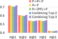
(a) MAG-CS, Cross-Encoder

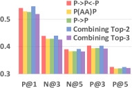
(b) PubMed, Cross-Encoder

Figure 6. P@$k$ and NDCG@$k$ scores of top-3 performing meta-paths/meta-graphs and the combination of them.

References

- (1)
- Agrawal et al. (2013) Rahul Agrawal, Archit Gupta, Yashoteja Prabhu, and Manik Varma. 2013. Multi-label learning with millions of labels: Recommending advertiser bid phrases for web pages. In WWW’13. 13–24.
- Beltagy et al. (2019) Iz Beltagy, Kyle Lo, and Arman Cohan. 2019. SciBERT: A Pretrained Language Model for Scientific Text. In EMNLP’19. 3615–3620.
- Chai et al. (2020) Duo Chai, Wei Wu, Qinghong Han, Fei Wu, and Jiwei Li. 2020. Description based text classification with reinforcement learning. In ICML’20. 1371–1382.
- Chalkidis et al. (2019) Ilias Chalkidis, Emmanouil Fergadiotis, Prodromos Malakasiotis, and Ion Androutsopoulos. 2019. Large-Scale Multi-Label Text Classification on EU Legislation. In ACL’19. 6314–6322.
- Chang et al. (2008) Ming-Wei Chang, Lev-Arie Ratinov, Dan Roth, and Vivek Srikumar. 2008. Importance of Semantic Representation: Dataless Classification.. In AAAI’08. 830–835.
- Chang et al. (2020) Wei-Cheng Chang, Hsiang-Fu Yu, Kai Zhong, Yiming Yang, and Inderjit S Dhillon. 2020. Taming pretrained transformers for extreme multi-label text classification. In KDD’20. 3163–3171.
- Chen et al. (2020) Ting Chen, Simon Kornblith, Mohammad Norouzi, and Geoffrey Hinton. 2020. A simple framework for contrastive learning of visual representations. In ICML’20. 1597–1607.
- Cohan et al. (2020) Arman Cohan, Sergey Feldman, Iz Beltagy, Doug Downey, and Daniel S Weld. 2020. SPECTER: Document-level Representation Learning using Citation-informed Transformers. In ACL’20. 2270–2282.
- Coletti and Bleich (2001) Margaret H Coletti and Howard L Bleich. 2001. Medical subject headings used to search the biomedical literature. JAMIA 8, 4 (2001), 317–323.
- Devlin et al. (2019) Jacob Devlin, Ming-Wei Chang, Kenton Lee, and Kristina Toutanova. 2019. BERT: Pre-training of Deep Bidirectional Transformers for Language Understanding. In NAACL-HLT’19. 4171–4186.
- Dong et al. (2017) Yuxiao Dong, Nitesh V Chawla, and Ananthram Swami. 2017. metapath2vec: Scalable representation learning for heterogeneous networks. In KDD’17. 135–144.
- Feng et al. (2021) Steven Y. Feng, Varun Gangal, Jason Wei, Sarath Chandar, Soroush Vosoughi, Teruko Mitamura, and Eduard Hovy. 2021. A Survey of Data Augmentation Approaches for NLP. In ACL Findings’21. 968–988.
- Gao et al. (2021a) Luyu Gao, Zhuyun Dai, and Jamie Callan. 2021a. Rethink Training of BERT Rerankers in Multi-stage Retrieval Pipeline. In ECIR’21. 280–286.
- Gao et al. (2021b) Tianyu Gao, Xingcheng Yao, and Danqi Chen. 2021b. SimCSE: Simple Contrastive Learning of Sentence Embeddings. In EMNLP’21. 6894–6910.
- Giorgi et al. (2021) John Giorgi, Osvald Nitski, Bo Wang, and Gary Bader. 2021. DeCLUTR: Deep Contrastive Learning for Unsupervised Textual Representations. In ACL’21. 879–895.
- Gupta et al. (2021) Nilesh Gupta, Sakina Bohra, Yashoteja Prabhu, Saurabh Purohit, and Manik Varma. 2021. Generalized Zero-Shot Extreme Multi-label Learning. In KDD’21. 527–535.
- Jain et al. (2019) Himanshu Jain, Venkatesh Balasubramanian, Bhanu Chunduri, and Manik Varma. 2019. Slice: Scalable linear extreme classifiers trained on 100 million labels for related searches. In WSDM’19. 528–536.
- Jain et al. (2016) Himanshu Jain, Yashoteja Prabhu, and Manik Varma. 2016. Extreme multi-label loss functions for recommendation, tagging, ranking & other missing label applications. In KDD’16. 935–944.
- Kim et al. (2019) Jihyeok Kim, Reinald Kim Amplayo, Kyungjae Lee, Sua Sung, Minji Seo, and Seung-won Hwang. 2019. Categorical Metadata Representation for Customized Text Classification. TACL 7 (2019), 201–215.
- Le and Mikolov (2014) Quoc Le and Tomas Mikolov. 2014. Distributed representations of sentences and documents. In ICML’14. 1188–1196.
- Lee et al. (2020) Jinhyuk Lee, Wonjin Yoon, Sungdong Kim, Donghyeon Kim, Sunkyu Kim, Chan Ho So, and Jaewoo Kang. 2020. BioBERT: a pre-trained biomedical language representation model for biomedical text mining. Bioinformatics 36, 4 (2020), 1234–1240.
- Liu et al. (2017) Jingzhou Liu, Wei-Cheng Chang, Yuexin Wu, and Yiming Yang. 2017. Deep learning for extreme multi-label text classification. In SIGIR’17. 115–124.
- Liu et al. (2019) Yinhan Liu, Myle Ott, Naman Goyal, Jingfei Du, Mandar Joshi, Danqi Chen, Omer Levy, Mike Lewis, Luke Zettlemoyer, and Veselin Stoyanov. 2019. Roberta: A robustly optimized bert pretraining approach. arXiv preprint arXiv:1907.11692 (2019).
- Lu (2011) Zhiyong Lu. 2011. PubMed and beyond: a survey of web tools for searching biomedical literature. Database 2011 (2011).
- Luo et al. (2021) Dongsheng Luo, Wei Cheng, Jingchao Ni, Wenchao Yu, Xuchao Zhang, Bo Zong, Yanchi Liu, Zhengzhang Chen, Dongjin Song, Haifeng Chen, et al. 2021. Unsupervised Document Embedding via Contrastive Augmentation. arXiv preprint arXiv:2103.14542 (2021).
- Medini et al. (2019) Tharun Kumar Reddy Medini, Qixuan Huang, Yiqiu Wang, Vijai Mohan, and Anshumali Shrivastava. 2019. Extreme Classification in Log Memory using Count-Min Sketch: A Case Study of Amazon Search with 50M Products. NeurIPS’19 (2019), 13265–13275.
- Mekala and Shang (2020) Dheeraj Mekala and Jingbo Shang. 2020. Contextualized Weak Supervision for Text Classification.. In ACL’20. 323–333.
- Mekala et al. (2020) Dheeraj Mekala, Xinyang Zhang, and Jingbo Shang. 2020. META: Metadata-Empowered Weak Supervision for Text Classification. In EMNLP’20. 8351–8361.
- Meng et al. (2018) Yu Meng, Jiaming Shen, Chao Zhang, and Jiawei Han. 2018. Weakly-supervised neural text classification. In CIKM’18. 983–992.
- Meng et al. (2020) Yu Meng, Yunyi Zhang, Jiaxin Huang, Chenyan Xiong, Heng Ji, Chao Zhang, and Jiawei Han. 2020. Weakly-Supervised Text Classification Using Label Names Only: A Language Model Self-Training Approach. In EMNLP’20. 9006–9017.
- Mikolov et al. (2013) Tomas Mikolov, Ilya Sutskever, Kai Chen, Greg S Corrado, and Jeff Dean. 2013. Distributed representations of words and phrases and their compositionality. In NIPS’13. 3111–3119.
- Mittal et al. (2021) Anshul Mittal, Noveen Sachdeva, Sheshansh Agrawal, Sumeet Agarwal, Purushottam Kar, and Manik Varma. 2021. ECLARE: Extreme Classification with Label Graph Correlations. In WWW’21. 3721–3732.
- Nam et al. (2016) Jinseok Nam, Eneldo Loza Mencía, and Johannes Fürnkranz. 2016. All-in text: Learning document, label, and word representations jointly. In AAAI’16. 1948–1954.
- Nam et al. (2015) Jinseok Nam, Eneldo Loza Mencía, Hyunwoo J Kim, and Johannes Fürnkranz. 2015. Predicting unseen labels using label hierarchies in large-scale multi-label learning. In ECML-PKDD’15. 102–118.
- Nogueira et al. (2019) Rodrigo Nogueira, Wei Yang, Kyunghyun Cho, and Jimmy Lin. 2019. Multi-stage document ranking with bert. arXiv preprint arXiv:1910.14424 (2019).
- Prabhu et al. (2018) Yashoteja Prabhu, Anil Kag, Shrutendra Harsola, Rahul Agrawal, and Manik Varma. 2018. Parabel: Partitioned label trees for extreme classification with application to dynamic search advertising. In WWW’18. 993–1002.
- Reimers and Gurevych (2019) Nils Reimers and Iryna Gurevych. 2019. Sentence-BERT: Sentence Embeddings using Siamese BERT-Networks. In EMNLP’19.
- Rios and Kavuluru (2018) Anthony Rios and Ramakanth Kavuluru. 2018. Few-shot and zero-shot multi-label learning for structured label spaces. In EMNLP’18, Vol. 2018. 3132.
- Robertson and Walker (1994) Stephen E Robertson and Steve Walker. 1994. Some simple effective approximations to the 2-poisson model for probabilistic weighted retrieval. In SIGIR’94. 232–241.
- Saini et al. (2021) Deepak Saini, Arnav Kumar Jain, Kushal Dave, Jian Jiao, Amit Singh, Ruofei Zhang, and Manik Varma. 2021. GalaXC: Graph Neural Networks with Labelwise Attention for Extreme Classification. In WWW’21. 3733–3744.
- Schulz et al. (2013) Axel Schulz, Aristotelis Hadjakos, Heiko Paulheim, Johannes Nachtwey, and Max Mühlhäuser. 2013. A multi-indicator approach for geolocalization of tweets. In ICWSM’13.
- Shen et al. (2021) Jiaming Shen, Wenda Qiu, Yu Meng, Jingbo Shang, Xiang Ren, and Jiawei Han. 2021. TaxoClass: Hierarchical Multi-Label Text Classification Using Only Class Names. In NAACL-HLT’21. 4239–4249.
- Shen et al. (2018) Zhihong Shen, Hao Ma, and Kuansan Wang. 2018. A Web-scale system for scientific knowledge exploration. In ACL’18, System Demonstrations. 87–92.
- Song and Roth (2014) Yangqiu Song and Dan Roth. 2014. On dataless hierarchical text classification. In AAAI’14. 1579–1585.
- Sun et al. (2011a) Yizhou Sun, Rick Barber, Manish Gupta, Charu C Aggarwal, and Jiawei Han. 2011a. Co-author relationship prediction in heterogeneous bibliographic networks. In ASONAM’11. 121–128.
- Sun and Han (2012) Yizhou Sun and Jiawei Han. 2012. Mining heterogeneous information networks: principles and methodologies. Synthesis Lectures on Data Mining and Knowledge Discovery 3, 2 (2012), 1–159.
- Sun et al. (2011b) Yizhou Sun, Jiawei Han, Xifeng Yan, Philip S Yu, and Tianyi Wu. 2011b. Pathsim: Meta path-based top-k similarity search in heterogeneous information networks. PVLDB 4, 11 (2011), 992–1003.
- Tang et al. (2015) Duyu Tang, Bing Qin, and Ting Liu. 2015. Learning semantic representations of users and products for document level sentiment classification. In ACL’15. 1014–1023.
- Wang et al. (2020b) Kuansan Wang, Zhihong Shen, Chiyuan Huang, Chieh-Han Wu, Yuxiao Dong, and Anshul Kanakia. 2020b. Microsoft academic graph: When experts are not enough. Quantitative Science Studies 1, 1 (2020), 396–413.
- Wang et al. (2019b) Wei Wang, Vincent W Zheng, Han Yu, and Chunyan Miao. 2019b. A survey of zero-shot learning: Settings, methods, and applications. ACM TIST 10, 2 (2019), 1–37.
- Wang et al. (2019a) Xiao Wang, Houye Ji, Chuan Shi, Bai Wang, Yanfang Ye, Peng Cui, and Philip S Yu. 2019a. Heterogeneous graph attention network. In WWW’19. 2022–2032.
- Wang et al. (2020a) Zihan Wang, Dheeraj Mekala, and Jingbo Shang. 2020a. X-Class: Text Classification with Extremely Weak Supervision. arXiv preprint arXiv:2010.12794 (2020).
- Wei and Zou (2019) Jason Wei and Kai Zou. 2019. EDA: Easy Data Augmentation Techniques for Boosting Performance on Text Classification Tasks. In EMNLP’19. 6382–6388.
- Wei and Li (2018) Tong Wei and Yu-Feng Li. 2018. Does tail label help for large-scale multi-label learning. In IJCAI’18. 2847–2853.
- Wei et al. (2021) Tong Wei, Wei-Wei Tu, Yu-Feng Li, and Guo-Ping Yang. 2021. Towards Robust Prediction on Tail Labels. In KDD’21. 1812–1820.
- Wu et al. (2020) Zhuofeng Wu, Sinong Wang, Jiatao Gu, Madian Khabsa, Fei Sun, and Hao Ma. 2020. Clear: Contrastive learning for sentence representation. arXiv preprint arXiv:2012.15466 (2020).
- Xie et al. (2020) Qizhe Xie, Zihang Dai, Eduard Hovy, Thang Luong, and Quoc Le. 2020. Unsupervised Data Augmentation for Consistency Training. NeurIPS’20 (2020).
- Yan et al. (2021) Yuanmeng Yan, Rumei Li, Sirui Wang, Fuzheng Zhang, Wei Wu, and Weiran Xu. 2021. ConSERT: A Contrastive Framework for Self-Supervised Sentence Representation Transfer. In ACL’21. 5065–5075.
- Yang et al. (2020) Carl Yang, Yuxin Xiao, Yu Zhang, Yizhou Sun, and Jiawei Han. 2020. Heterogeneous network representation learning: A unified framework with survey and benchmark. IEEE TKDE (2020).
- Yen et al. (2017) Ian EH Yen, Xiangru Huang, Wei Dai, Pradeep Ravikumar, Inderjit Dhillon, and Eric Xing. 2017. Ppdsparse: A parallel primal-dual sparse method for extreme classification. In KDD’17. 545–553.
- Yin et al. (2019) Wenpeng Yin, Jamaal Hay, and Dan Roth. 2019. Benchmarking Zero-shot Text Classification: Datasets, Evaluation and Entailment Approach. In EMNLP’19. 3905–3914.
- You et al. (2019) Ronghui You, Zihan Zhang, Ziye Wang, Suyang Dai, Hiroshi Mamitsuka, and Shanfeng Zhu. 2019. Attentionxml: Label tree-based attention-aware deep model for high-performance extreme multi-label text classification. NeurIPS’19 (2019), 5820–5830.
- Zhang et al. (2018) Daokun Zhang, Jie Yin, Xingquan Zhu, and Chengqi Zhang. 2018. Metagraph2vec: Complex semantic path augmented heterogeneous network embedding. In PAKDD’18. 196–208.
- Zhang et al. (2021d) Xinyang Zhang, Chenwei Zhang, Xin Luna Dong, Jingbo Shang, and Jiawei Han. 2021d. Minimally-Supervised Structure-Rich Text Categorization via Learning on Text-Rich Networks. In WWW’21. 3258–3268.
- Zhang et al. (2021a) Yu Zhang, Xiusi Chen, Yu Meng, and Jiawei Han. 2021a. Hierarchical Metadata-Aware Document Categorization under Weak Supervision. In WSDM’21. 770–778.
- Zhang et al. (2021b) Yu Zhang, Shweta Garg, Yu Meng, Xiusi Chen, and Jiawei Han. 2021b. MotifClass: Weakly Supervised Text Classification with Higher-order Metadata Information. arXiv preprint arXiv:2111.04022 (2021).
- Zhang et al. (2020) Yu Zhang, Yu Meng, Jiaxin Huang, Frank F. Xu, Xuan Wang, and Jiawei Han. 2020. Minimally Supervised Categorization of Text with Metadata. In SIGIR’20. 1231–1240.
- Zhang et al. (2021c) Yu Zhang, Zhihong Shen, Yuxiao Dong, Kuansan Wang, and Jiawei Han. 2021c. MATCH: Metadata-Aware Text Classification in A Large Hierarchy. In WWW’21. 3246–3257.
- Zhang et al. (2017) Yu Zhang, Wei Wei, Binxuan Huang, Kathleen M Carley, and Yan Zhang. 2017. RATE: Overcoming Noise and Sparsity of Textual Features in Real-Time Location Estimation. In CIKM’17. 2423–2426.
- Zhang et al. (2019) Yu Zhang, Frank F. Xu, Sha Li, Yu Meng, Xuan Wang, Qi Li, and Jiawei Han. 2019. HiGitClass: Keyword-Driven Hierarchical Classification of GitHub Repositories. In ICDM’19. 876–885.