Based on a talk given at the Nankai Symposium on Mathematical Dialogues 2021

Abstract

Calabi–Yau manifolds have played a key role in both mathematics and physics, and are particularly important for deriving realistic models of particle physics from string theory. Unfortunately, very little is known about the explicit metrics on these spaces, leaving us unable, for example, to compute particle masses or couplings in these models. We review recent progress in this direction on using numerical approximations to compute the spectrum of the Laplacian on these spaces. We give an example of what one can do with this new “data”, giving a surprising link between Calabi–Yau metrics and random matrix theory.

1 Introduction and summary

Calabi–Yau manifolds have a rich mathematical history and give a starting point for recovering realistic four-dimensional physics from string theory. Despite much study, there are still no explicit expressions for non-trivial Ricci-flat metrics on these spaces. Viewed from the string worldsheet, these manifolds define interacting two-dimensional superconformal field theories (SCFTs). These theories come in families labelled by the complex structure and Kähler moduli of the underlying Calabi–Yau. In the large-volume limit, these theories are described by non-linear $\sigma$-models whose target space is simply the Calabi–Yau equipped with its Ricci-flat metric.

Recent advances in numerical methods give us access to both the Ricci-flat metric and the spectrum of the Laplacian on these spaces. The spectrum is an source of new non-BPS “data” which characterises CFT operators with low scaling dimension. In this talk, we show that the spectrum of the Laplacian, and thus the spectrum of operators in the corresponding CFT, averaged over complex structure moduli displays the hallmarks of chaos in the form of random matrix statistics. In our companion paper [4], we also examine K3 CFTs and the spectra of field theories on genus-three Riemann surfaces, again finding chaos in their spectra.

Further work includes extending our analysis to the non-scalar spectrum, understanding the interplay of the explicit spectrum with the conformal [5, 6, 7, 8, 9, 10, 11] and geometric [12, 13, 14, 15] bootstrap programmes, exploring whether RMT sheds light on interacting CFTs in an averaged sense or if it can be used to understand the “typical” properties of Calabi–Yau compactifications [16, 17, 18, 19, 20, 21, 22]

A point to emphasise is that one could imagine taking random metrics on these manifolds and finding similar random matrix statistics. Our surprising result is that one sees this chaotic behaviour even within the restricted class of Ricci-flat metrics on a Calabi–Yau hypersurface. A related observation is that one sees similar behaviour for constant negative curvature metrics on genus-three Riemann surfaces. In this context, there are mathematical theorems relating the behaviour of geodesics to chaotic particle motion on these manifolds [23, 24, 25, 26]. This suggests that something similar should be true for Ricci-flat metrics, though this still appears to be an open question.

2 Chaos in 2d CFTs from Calabi–Yau $\sigma$-models?

Even in two dimensions, very little is known about the spectrum of interacting CFTs. For CFTs at generic points in moduli space, one can study quantities protected by supersymmetry [27, 28, 29, 30, 31, 32, 33, 34] or use modular invariance and the conformal bootstrap to constrain the spectrum in some way [5, 6, 7, 8, 9, 10]. In general, however, there is no way to compute the spectrum of an interacting CFT.

There are large families of SCFTs defined by Calabi–Yau manifolds. For example, a $(2,2)$ $\sigma$-model with a Calabi–Yau threefold target space $X$ is known to flow to a $(2,2)$ SCFT [35, 36, 37], with the complex structure and Kähler moduli of the Calabi–Yau metric determining certain exactly marginal couplings in the field theory [38, 39, 40, 41, 42, 43].

The relation of the geometry of the Calabi–Yau to the spectrum of operators in the CFT was given first by Witten [27]. At low energies, the $\sigma$-model reduces to a quantum mechanics for a point particle moving on the target space, with the Hamiltonian given by the de Rham Laplacian, $\Delta$, for the Ricci-flat metric. Thanks to this, one can study the low-lying operators of the CFT via the geometry of the Calabi–Yau. Primary operators $\{\mathcal{O}_{i}\}$ in the CFT are eigenstates of the Hamiltonian with fixed scaling dimension $D_{i}$:

$$H|\mathcal{O}_{i}\rangle=D_{i}|\mathcal{O}_{i}\rangle,\qquad D_{i}\geq 0,$$ (2.1)

In the large-volume limit, these operators correspond to the $(p,q)$-eigenforms of $\Delta$, with scaling dimensions

$$D=\lambda+\frac{p+q}{2},$$ (2.2)

where $\lambda$ is the eigenvalue of the corresponding eigenform. Since $\lambda\sim\operatorname{Vol}(X)^{-1/\dim_{\mathbb{C}}X}$, at large volume the light operators come from scalar eigenmodes of $\Delta$.

In the spirit of “experimental” theoretical physics, we ask the following question:

Given an ensemble of CFTs, do the scaling dimensions $\{D_{i}\}$ of primary operators display any interesting statistics? In particular, do they display signs of chaos?

This is obviously a difficult question to answer: we need families of generic, interacting CFTs, and we have to be able to compute the spectrum of these theories. The requirement of being generic and interacting immediately rules out looking at solvable or rational CFTs, and needing families of such theories means we cannot look at special points in moduli space or isolated CFTs, such as the Ising model.

Until recently, it was not possible to answer such a question, other than in free field theories [44, 45, 46]. The idea we pursue in this talk is to construct an ensemble of CFTs and compute their spectra numerically via the connection to Calabi–Yau geometries. We then analyse the spectra statistically and find that they display random matrix statistics, indicative of chaos in the underlying field theory.

3 Numerical Calabi–Yau metrics and their spectra

Calabi–Yau (CY) manifolds are Kähler manifolds which admit Ricci-flat metrics. Thanks to Yau’s proof [47] of the Calabi conjecture [48], we know that such metrics exist when $c_{1}(X)=0$. This proof is in no way constructive, however, and so the metrics must be determined by other means.

There are now many methods to compute numerical approximations to Ricci-flat metrics on CY manifolds [49, 50, 51, 52, 53, 54, 55, 56, 57, 58, 59, 60, 61], which have been discussed many times in the literature [51, 62, 63, 64, 65, 66, 67, 68, 69, 70, 71, 72]. In this work, we use an algorithm due to Donaldson [51], based on the algebraic metrics ansatz of Tian [50]. One iteratively solves for a balanced metric on $X$, which is known to approach the Ricci-flat metric in a certain limit. In practice, this involves converting integrals over $X$ to discrete sums – one uses Monte Carlo methods to implement this using a sampling method discussed in [63, 64].

3.1 The Laplacian on a Calabi–Yau

In the large-volume limit, low-lying operators in the CFT are determined by scalar eigenmodes on the CY. These eigenmodes satisfy

$$\Delta\phi_{n}=\lambda_{n}\phi_{n},\qquad\Delta=\delta\text{d}.$$ (3.1)

Given the data of an approximate CY metric, we can then calculate the spectrum $\{\lambda_{n}\}$ following [73, 74, 68, 75]. We do this by expanding the eigenmodes in a truncated, finite basis of functions $\{\alpha_{A}\}$, so that $\phi=\phi_{A}\alpha_{A}$, thus giving a finite-dimensional generalised eigenvalue problem,

$$\Delta_{AB}\phi_{B}=\lambda\,O_{AB}\phi_{B},$$ (3.2)

where $\Delta_{AB}=\langle\alpha_{A},\Delta\alpha_{B}\rangle$ and $O_{AB}=\langle\alpha_{A},\alpha_{B}\rangle$ both depend on the approximate CY metric.

4 Calabi–Yau CFTs and random matrix theory

A suitable ensemble of CFTs is provided by constructing a family of CY manifolds with varying complex structure moduli. For example, a generic quintic threefold $X$ is defined by a quintic equation in $\mathbb{P}^{4}$ with coordinates $[z_{0}\!:\!\dots\!:\!z_{4}]$:

$$X\equiv\sum_{m,n,p,q,r}c_{mnpqr}z_{m}z_{n}z_{p}z_{q}z_{r}=0.$$ (4.1)

This describes a 101-dimensional family of CYs. We sample the $c_{mnpqr}$ randomly from the unit disk in the complex plane with a flat measure:

$$c_{mnpqr}\in\mathbb{C},\qquad|c_{mnpqr}|<1.$$ (4.2)

For each choice of complex structure moduli, we compute an approximate Ricci-flat metric and the spectrum of the Laplacian numerically. This gives us an ensemble of spectra which can be interpreted as an ensemble of scaling dimensions of operators in the large-volume CFT.

Since we are looking for signs of chaos in the spectrum of CFTs, it is useful to have some diagnostics of chaotic behaviour. In our case, we take random matrix statistics to be indicative of chaos in the spectrum [76, 77, 78, 79, 80, 81].

4.1 Random matrix theory and spectral statistics

Random matrix theory (RMT) is the study of the distribution of eigenvalues of matrices whose entries are independent and identically distributed random variables. RMT governs many physical systems, such as nuclear physics [82, 83, 84, 85], billiards [80, 86, 87], quantum many-body systems such as the SYK model [88, 89, 90, 91], and toy models of black-hole physics and quantum gravity [92, 93, 94, 95, 96]. The latter suggests, via holography, that generic conformal field theories may also display signs of chaos.

We will compare the statistics of scaling dimensions of primary operators with the eigenvalue statistics of a random matrix theory, specifically the Gaussian orthogonal ensemble (GOE). This is the ensemble of eigenvalues of $N\times N$ real, symmetric matrices, where the entries of the matrices are independently drawn from a Gaussian distribution. We will focus on universal features of random matrix theory by unfolding, letting us focus on the statistics of fluctuations in the spectrum.

We measure RMT behaviour via three diagnostics: the nearest-neighbour level spacing $p_{1}(s)$, the number variance $\Sigma^{2}(L)$, and the spectral form factor $S(t,\beta)$. Together, these provide measures of both long- and short-range correlations in the spectrum [76, 79].

The nearest-neighbour level spacing is the probability of two consecutive eigenvalues being separated by a distance $s$. For the GOE in the large-$N$ limit, it is

$$p_{1}(s)=\frac{\pi}{2}s\,\text{e}^{-\pi s^{2}/4}.$$ (4.3)

The maximum of this distribution is away from $s=0$, indicative of eigenvalue repulsion. The number variance is the fluctuation of the number of eigenvalues averaged over an interval of size $L$. For the GOE, it scales as

$$\Sigma^{2}(L)\sim\log L.$$ (4.4)

The logarithmic growth is an indication of spectral rigidity. The spectral form factor (SFF) (up to an overall normalisation) is the analytically continued thermal partition [97]

$$S(t,\beta)\sim\biggl{|}\sum_{n}\text{e}^{-(\beta+2\pi\text{i}t)\lambda_{n}}\biggr{|}^{2}.$$ (4.5)

The spectral form factor displays three characteristic features: a dip with ringing for finite $N$, a ramp, and a plateau. We show these features for the GOE in Figure 1.

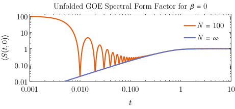
Figure 1: Unfolded GOE spectral form factors for $\beta=0$. The orange curve is computed from 100,000, $100\times 100$ random symmetric matrices. The blue curve shows the SFF for $N\to\infty$ and $\beta\to 0$ – only the ramp and plateau are present.

4.2 Results

We generated 1,000 different samples of quintic threefolds of the form (4.1), with complex structure moduli given by random choices of $c_{mnpqr}$. For each sample, we keep the lowest-lying 100 eigenvalues of the Laplacian. We then repeat this for 1,000 different choices of the $c_{mnpqr}$, and analyse the resulting distribution of operator scaling dimensions.

We compare the distribution of scaling dimensions with the distribution of eigenvalues from a random matrix ensemble in Figure 2. The SFF shows the characteristic dip with ringing, ramp and plateau. The ramp shows a smooth transition to the plateau region, suggesting GOE statistics. The nearest-neighbour level spacing and number variance also match those of the GOE.

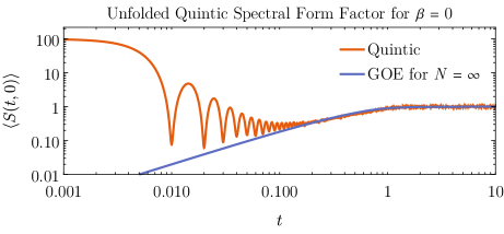
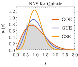
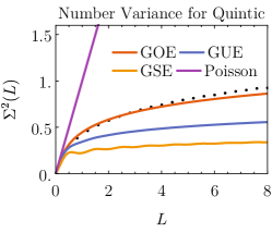
Figure 2: The first row shows the unfolded spectral form factor for $\beta=0$ for quintic Calabi–Yau threefolds. The orange curve shows an ensemble average consisting of 1,000 samples with varying complex structure, with each sample containing the 100 lowest-lying eigenvalues. The dip, ramp and plateau are all present. The second row shows the nearest-neighbour level spacings (NNS) and the number variance, together with fits to GOE. Other matrix ensembles are shown for comparison.

Acknowledgements

We thank Nima Afkhami-Jeddi and Clay Córdova for collaboration on the project which this article is based upon. AA is supported by the European Union’s Horizon 2020 research and innovation program under the Marie Skłodowska-Curie grant agreement No. 838776. This work was completed in part with resources provided by the University of Chicago Research Computing Center.

References

- [1] S. Kachru, A. Tripathy, and M. Zimet, “K3 metrics from little string theory”, arXiv:1810.10540 [hep-th].
- [2] S. Kachru, A. Tripathy, and M. Zimet, “K3 metrics”, arXiv:2006.02435 [hep-th].
- [3] A. Tripathy and M. Zimet, “A plethora of K3 metrics”, arXiv:2010.12581 [hep-th].
- [4] N. Afkhami-Jeddi, A. Ashmore, and C. Cordova, “Calabi-Yau CFTs and Random Matrices”, arXiv:2107.11461 [hep-th].
- [5] S. Hellerman, “A Universal Inequality for CFT and Quantum Gravity”, JHEP 08 (2011)130, arXiv:0902.2790 [hep-th].
- [6] C. A. Keller and H. Ooguri, “Modular Constraints on Calabi-Yau Compactifications”, Commun. Math. Phys. 324 (2013)107–127, arXiv:1209.4649 [hep-th].
- [7] D. Friedan and C. A. Keller, “Constraints on 2d CFT partition functions”, JHEP 10 (2013)180, arXiv:1307.6562 [hep-th].
- [8] Y.-H. Lin, S.-H. Shao, D. Simmons-Duffin, Y. Wang, and X. Yin, “ = 4 superconformal bootstrap of the K3 CFT”, JHEP 05 (2017)126, arXiv:1511.04065 [hep-th].
- [9] S. Collier, Y.-H. Lin, and X. Yin, “Modular Bootstrap Revisited”, JHEP 09 (2018)061, arXiv:1608.06241 [hep-th].
- [10] Y.-H. Lin, S.-H. Shao, Y. Wang, and X. Yin, “(2, 2) superconformal bootstrap in two dimensions”, JHEP 05 (2017)112, arXiv:1610.05371 [hep-th].
- [11] P. Kravchuk, D. Mazac, and S. Pal, “Automorphic Spectra and the Conformal Bootstrap”, arXiv:2111.12716 [hep-th].
- [12] J. Bonifacio and K. Hinterbichler, “Unitarization from Geometry”, JHEP 12 (2019)165, arXiv:1910.04767 [hep-th].
- [13] J. Bonifacio and K. Hinterbichler, “Bootstrap Bounds on Closed Einstein Manifolds”, JHEP 10 (2020)069, arXiv:2007.10337 [hep-th].
- [14] J. Bonifacio, “Bootstrap Bounds on Closed Hyperbolic Manifolds”, arXiv:2107.09674 [hep-th].
- [15] J. Bonifacio, “Bootstrapping Closed Hyperbolic Surfaces”, arXiv:2111.13215 [hep-th].
- [16] S. Ashok and M. R. Douglas, “Counting flux vacua”, JHEP 01 (2004)060, arXiv:hep-th/0307049.
- [17] M. R. Douglas, B. Shiffman, and S. Zelditch, “Critical points and supersymmetric vacua”, Commun. Math. Phys. 252 (2004)325–358, arXiv:math/0402326.
- [18] M. R. Douglas, “The Statistics of string / M theory vacua”, JHEP 05 (2003)046, arXiv:hep-th/0303194.
- [19] F. Denef and M. R. Douglas, “Distributions of flux vacua”, JHEP 05 (2004)072, arXiv:hep-th/0404116.
- [20] F. Denef and M. R. Douglas, “Distributions of nonsupersymmetric flux vacua”, JHEP 03 (2005)061, arXiv:hep-th/0411183.
- [21] J. Distler and U. Varadarajan, “Random polynomials and the friendly landscape”, arXiv:hep-th/0507090.
- [22] D. I. Podolsky, J. Majumder, and N. Jokela, “Disorder on the landscape”, JCAP 05 (2008)024, arXiv:0804.2263 [hep-th].
- [23] G. A. Hedlund, “On the metrical transitivity of the geodesics on closed surfaces of constant negative curvature”, Annals of Mathematics 35 4, (1934)787–808.
- [24] E. Hopf, “Ergodic theory and the geodesic flow on surfaces of constant negative curvature”, Bulletin of the American Mathematical Society 77 6, (1971)863 – 877.
- [25] E. Hopf, “Statistik der geodätischen Linien in Mannigfaltigkeiten negativer Krümmung”, Ber. Verh. Sächs. Akad. Wiss. 91 (1939)261–304.
- [26] G. A. Hedlund, “Geodesic flows on closed riemann manifolds with negative curvature”, Proceedings of the Steklov Institute of Mathematics 90, (1967).
- [27] E. Witten, “Constraints on Supersymmetry Breaking”, Nucl. Phys. B 202 (1982)253.
- [28] T. Eguchi and A. Taormina, “Character Formulas for the Superconformal Algebra”, Phys. Lett. B 200 (1988)315.
- [29] T. Eguchi, H. Ooguri, A. Taormina, and S.-K. Yang, “Superconformal Algebras and String Compactification on Manifolds with SU(N) Holonomy”, Nucl. Phys. B 315 (1989)193–221.
- [30] S. Cecotti, P. Fendley, K. A. Intriligator, and C. Vafa, “A New supersymmetric index”, Nucl. Phys. B 386 (1992)405–452, arXiv:hep-th/9204102.
- [31] T. Kawai, Y. Yamada, and S.-K. Yang, “Elliptic genera and N=2 superconformal field theory”, Nucl. Phys. B 414 (1994)191–212, arXiv:hep-th/9306096.
- [32] R. Dijkgraaf, E. P. Verlinde, and H. L. Verlinde, “Counting dyons in N=4 string theory”, Nucl. Phys. B 484 (1997)543–561, arXiv:hep-th/9607026.
- [33] F. Benini, R. Eager, K. Hori, and Y. Tachikawa, “Elliptic genera of two-dimensional N=2 gauge theories with rank-one gauge groups”, Lett. Math. Phys. 104 (2014)465–493, arXiv:1305.0533 [hep-th].
- [34] Y.-H. Lin, S.-H. Shao, Y. Wang, and X. Yin, “Supersymmetry Constraints and String Theory on K3”, JHEP 12 (2015)142, arXiv:1508.07305 [hep-th].
- [35] C. M. Hull, “ULTRAVIOLET FINITENESS OF SUPERSYMMETRIC NONLINEAR SIGMA MODELS”, Nucl. Phys. B 260 (1985)182–202.
- [36] L. Alvarez-Gaume, S. R. Coleman, and P. H. Ginsparg, “Finiteness of Ricci Flat Supersymmetric Models”, Commun. Math. Phys. 103 (1986)423.
- [37] D. Nemeschansky and A. Sen, “Conformal Invariance of Supersymmetric Models on Calabi-yau Manifolds”, Phys. Lett. B 178 (1986)365–369.
- [38] D. Friedan, “Nonlinear Models in Two Epsilon Dimensions”, Phys. Rev. Lett. 45 (1980)1057.
- [39] L. Alvarez-Gaume and D. Z. Freedman, “Geometrical Structure and Ultraviolet Finiteness in the Supersymmetric Sigma Model”, Commun. Math. Phys. 80 (1981)443.
- [40] L. Alvarez-Gaume and D. Z. Freedman, “Kahler Geometry and the Renormalization of Supersymmetric Sigma Models”, Phys. Rev. D 22 (1980)846.
- [41] L. Alvarez-Gaume, D. Z. Freedman, and S. Mukhi, “The Background Field Method and the Ultraviolet Structure of the Supersymmetric Nonlinear Sigma Model”, Annals Phys. 134 (1981)85.
- [42] L. Alvarez-Gaume and P. H. Ginsparg, “Finiteness of Ricci Flat Supersymmetric Nonlinear Sigma Models”, Commun. Math. Phys. 102 (1985)311.
- [43] D. J. Gross and E. Witten, “Superstring Modifications of Einstein’s Equations”, Nucl. Phys. B 277 (1986)1.
- [44] N. Afkhami-Jeddi, H. Cohn, T. Hartman, and A. Tajdini, “Free partition functions and an averaged holographic duality”, JHEP 01 (2021)130, arXiv:2006.04839 [hep-th].
- [45] A. Maloney and E. Witten, “Averaging over Narain moduli space”, JHEP 10 (2020)187, arXiv:2006.04855 [hep-th].
- [46] N. Benjamin, C. A. Keller, H. Ooguri, and I. G. Zadeh, “Narain to Narnia”, arXiv:2103.15826 [hep-th].
- [47] S. T. Yau, “On the Ricci curvature of a compact Kähler manifold and the complex Monge-Ampère equation.I.”, Commun. Pure Appl. Math. 31 3, (1978)339–411.
- [48] E. Calabi and K. On, “On kähler manifolds with vanishing canonical class”, Princeton Mathematical Series 12 (1957)78–89.
- [49] M. Headrick and T. Wiseman, “Numerical Ricci-flat metrics on K3”, Class. Quant. Grav. 22 (2005)4931–4960, arXiv:hep-th/0506129.
- [50] G. Tian, “On a set of polarized Kähler metrics on algebraic manifolds”, Journal of Differential Geometry 32 1, (1990)99 – 130.
- [51] S. Donaldson, “Some numerical results in complex differential geometry”, Pure and Applied Mathematics Quarterly 5 2, (2009)571–618, arXiv:math/0512625 [math.DG].
- [52] M. R. Douglas, R. L. Karp, S. Lukic, and R. Reinbacher, “Numerical Calabi-Yau metrics”, J. Math. Phys. 49 (2008)032302, arXiv:hep-th/0612075.
- [53] V. Braun, T. Brelidze, M. R. Douglas, and B. A. Ovrut, “Calabi-Yau Metrics for Quotients and Complete Intersections”, JHEP 05 (2008)080, arXiv:0712.3563 [hep-th].
- [54] M. Headrick and A. Nassar, “Energy functionals for Calabi-Yau metrics”, Adv. Theor. Math. Phys. 17 5, (2013)867–902, arXiv:0908.2635 [hep-th].
- [55] A. Ashmore, Y.-H. He, and B. A. Ovrut, “Machine Learning Calabi–Yau Metrics”, Fortsch. Phys. 68 9, (2020)2000068, arXiv:1910.08605 [hep-th].
- [56] L. B. Anderson, M. Gerdes, J. Gray, S. Krippendorf, N. Raghuram, and F. Ruehle, “Moduli-dependent Calabi-Yau and SU(3)-structure metrics from Machine Learning”, JHEP 05 (2021)013, arXiv:2012.04656 [hep-th].
- [57] M. R. Douglas, S. Lakshminarasimhan, and Y. Qi, “Numerical Calabi-Yau metrics from holomorphic networks”, arXiv:2012.04797 [hep-th].
- [58] V. Jejjala, D. K. Mayorga Pena, and C. Mishra, “Neural Network Approximations for Calabi-Yau Metrics”, arXiv:2012.15821 [hep-th].
- [59] M. R. Douglas, “Holomorphic feedforward networks”, arXiv:2105.03991 [math.CV].
- [60] M. Larfors, A. Lukas, F. Ruehle, and R. Schneider, “Learning Size and Shape of Calabi-Yau Spaces”, arXiv:2111.01436 [hep-th].
- [61] A. Ashmore, L. Calmon, Y.-H. He, and B. A. Ovrut, “Calabi-Yau Metrics, Energy Functionals and Machine-Learning”, arXiv:2112.10872 [hep-th].
- [62] M. Headrick and T. Wiseman, “Numerical Ricci-flat metrics on K3”, Class. Quant. Grav. 22 (2005)4931–4960, arXiv:hep-th/0506129.
- [63] M. R. Douglas, R. L. Karp, S. Lukic, and R. Reinbacher, “Numerical Calabi-Yau metrics”, J. Math. Phys. 49 (2008)032302, arXiv:hep-th/0612075.
- [64] V. Braun, T. Brelidze, M. R. Douglas, and B. A. Ovrut, “Calabi-Yau Metrics for Quotients and Complete Intersections”, JHEP 05 (2008)080, arXiv:0712.3563 [hep-th].
- [65] M. Headrick and A. Nassar, “Energy functionals for Calabi-Yau metrics”, Adv. Theor. Math. Phys. 17 5, (2013)867–902, arXiv:0908.2635 [hep-th].
- [66] A. Ashmore, Y.-H. He, and B. A. Ovrut, “Machine Learning Calabi–Yau Metrics”, Fortsch. Phys. 68 9, (2020)2000068, arXiv:1910.08605 [hep-th].
- [67] W. Cui and J. Gray, “Numerical Metrics, Curvature Expansions and Calabi-Yau Manifolds”, JHEP 05 (2020)044, arXiv:1912.11068 [hep-th].
- [68] A. Ashmore, “Eigenvalues and eigenforms on Calabi-Yau threefolds”, arXiv:2011.13929 [hep-th].
- [69] L. B. Anderson, M. Gerdes, J. Gray, S. Krippendorf, N. Raghuram, and F. Ruehle, “Moduli-dependent Calabi-Yau and SU(3)-structure metrics from Machine Learning”, JHEP 05 (2021)013, arXiv:2012.04656 [hep-th].
- [70] M. R. Douglas, S. Lakshminarasimhan, and Y. Qi, “Numerical Calabi-Yau metrics from holomorphic networks”, arXiv:2012.04797 [hep-th].
- [71] V. Jejjala, D. K. Mayorga Pena, and C. Mishra, “Neural Network Approximations for Calabi-Yau Metrics”, arXiv:2012.15821 [hep-th].
- [72] A. Ashmore, R. Deen, Y.-H. He, and B. A. Ovrut, “Machine Learning Line Bundle Connections”, arXiv:2110.12483 [hep-th].
- [73] C. Iuliu-Lazaroiu, D. McNamee, and C. Saemann, “Generalized Berezin quantization, Bergman metrics and fuzzy Laplacians”, JHEP 09 (2008)059, arXiv:0804.4555 [hep-th].
- [74] V. Braun, T. Brelidze, M. R. Douglas, and B. A. Ovrut, “Eigenvalues and Eigenfunctions of the Scalar Laplace Operator on Calabi-Yau Manifolds”, JHEP 07 (2008)120, arXiv:0805.3689 [hep-th].
- [75] A. Ashmore and F. Ruehle, “Moduli-dependent KK towers and the swampland distance conjecture on the quintic Calabi-Yau manifold”, Phys. Rev. D 103 10, (2021)106028, arXiv:2103.07472 [hep-th].
- [76] M. Mehta, Random Matrices, vol. 142 of Pure and Applied Mathematics. Elsevier/Academic Press, 2004.
- [77] E. Brézin and S. Hikami, “Spectral form factor in a random matrix theory”, Phys. Rev. E 55 (1997)4067–4083.
- [78] T. A. Brody, J. Flores, J. B. French, P. A. Mello, A. Pandey, and S. S. M. Wong, “Random-matrix physics: spectrum and strength fluctuations”, Rev. Mod. Phys. 53 (1981)385–479.
- [79] T. Guhr, A. Muller-Groeling, and H. A. Weidenmuller, “Random matrix theories in quantum physics: Common concepts”, Phys. Rept. 299 (1998)189–425, arXiv:cond-mat/9707301.
- [80] O. Bohigas, M. J. Giannoni, and C. Schmit, “Characterization of chaotic quantum spectra and universality of level fluctuation laws”, Phys. Rev. Lett. 52 (Jan, 1984)1–4.
- [81] O. Bohigas, M. Giannoni, and C. Schmit, “Spectral properties of the laplacian and random matrix theories”, Journal de Physique Lettres 45 21, (1984)1015–1022.
- [82] E. P. Wigner, “Characteristic vectors of bordered matrices with infinite dimensions”, Annals of Mathematics 62 3, (1955)548–564.
- [83] N. Rosenzweig and C. E. Porter, ““Repulsion of energy levels” in complex atomic spectra”, Phys. Rev. 120 (Dec, 1960)1698–1714.
- [84] R. E. Trees, ““Repulsion of energy levels” in complex atomic spectra”, Phys. Rev. 123 (Aug, 1961)1293–1300.
- [85] R. Haq, A. Pandey, and O. Bohigas, “Fluctuation properties of nuclear energy levels: Do theory and experiment agree?”, Physical Review Letters 48 16, (1982)1086–1089.
- [86] M. C. Gutzwiller, Chaos in Classical and Quantum Mechanics. Springer New York, 1990.
- [87] N. Balazs and A. Voros, “Chaos on the pseudosphere”, Physics Reports 143 3, (1986)109–240.
- [88] S. Sachdev and J. Ye, “Gapless spin fluid ground state in a random, quantum Heisenberg magnet”, Phys. Rev. Lett. 70 (1993)3339, arXiv:cond-mat/9212030.
- [89] A. Kitaev, “Hidden correlations in the Hawking radiation and thermal noise”, 1998. https://online.kitp.ucsb.edu/online/joint98/kitaev/.
- [90] A. Kitaev, “A simple model of quantum holography I”, 2015. https://online.kitp.ucsb.edu/online/entangled15/kitaev/.
- [91] A. Kitaev, “A simple model of quantum holography II”, 2015. https://online.kitp.ucsb.edu/online/entangled15/kitaev2/.
- [92] P. Saad, S. H. Shenker, and D. Stanford, “A semiclassical ramp in SYK and in gravity”, arXiv:1806.06840 [hep-th].
- [93] A. M. García-García and J. J. M. Verbaarschot, “Spectral and thermodynamic properties of the Sachdev-Ye-Kitaev model”, Phys. Rev. D 94 12, (2016)126010, arXiv:1610.03816 [hep-th].
- [94] Y.-Z. You, A. W. W. Ludwig, and C. Xu, “Sachdev-Ye-Kitaev model and thermalization on the boundary of many-body localized fermionic symmetry-protected topological states”, Phys. Rev. B 95 (Mar, 2017)115150, arXiv:1602.06964 [cond-mat.str-el].
- [95] J. S. Cotler, G. Gur-Ari, M. Hanada, J. Polchinski, P. Saad, S. H. Shenker, D. Stanford, A. Streicher, and M. Tezuka, “Black Holes and Random Matrices”, JHEP 05 (2017)118, arXiv:1611.04650 [hep-th]. [Erratum: JHEP 09, 002 (2018)].
- [96] H. Gharibyan, M. Hanada, S. H. Shenker, and M. Tezuka, “Onset of Random Matrix Behavior in Scrambling Systems”, JHEP 07 (2018)124, arXiv:1803.08050 [hep-th]. [Erratum: JHEP 02, 197 (2019)].
- [97] F. Haake, Quantum Signatures of Chaos. Springer Series in Synergetics. Springer, Berlin, Heidelberg, 3 ed., 2010.