Particle production during inflation: A Bayesian analysis with CMB data from Planck 2018

Abstract

A class of inflationary models that involve rapid bursts of particle productions predict observational signatures, such as bump-like features in the primordial scalar power spectrum. In this work, we analyze such models by comparing their predictions with the latest CMB data from Planck 2018. We consider two scenarios of particle production. The first one is a simple scenario consisting of a single burst of particle production during observable inflation. The second one consists of multiple bursts of particle production that lead to a series of bump-like features in the primordial power spectrum. We find that the second scenario of the multi-bump model gives better fit to the CMB data compared to the concordance $\Lambda$CDM model. We carried out model comparisons using Bayesian evidences. From the observational constraints on the amplitude of primordial features of the multi-bump model, we find that the dimensionless coupling parameter $g$ responsible for particle production is bound to be $g<0.05$.

1 Introduction

Cosmic inflation [1, 2, 3, 4, 5, 6] is the hypothetical accelerated expansion in the early universe, which was proposed to explain the unnatural initial conditions of the Big Bang model. The relevant energy scale of the inflationary era is so high that any observations are beyond the reach of direct exploration. However, modeling cosmic inflation and predicting its signatures in cosmological observations provides an alternative indirect strategy to understand the physics at such high energy scales. The observations of density fluctuations provide valuable information about the history of the universe. According to the inflationary scenario, the seeds of the density fluctuations were supposed to have been created during inflation. Hence, the fluctuations in the distribution of matter and radiation that we observe today are expected to contain important clues about how inflation happened. Due to the high energy scale involved, the cosmic inflation must be described by a particle physics model beyond the Standard Model.

A plethora of inflationary models have been proposed over the years and tested using cosmological observations such as Cosmic Microwave Background (CMB) radiation and matter distributions. The tests provide constraints on the parameters of the underlying theoretical models. Cosmological observations have suggested that our universe can be modeled accurately by the concordance $\Lambda$CDM model. This model successfully explains a wide range of cosmological phenomena with just six parameters. The concordance model assumes an almost scale-invariant primordial power spectrum of scalar perturbations characterized by only two parameters: the amplitude of the perturbations and the spectral tilt of the power spectrum. Any hint of disagreement between the concordance model and observations may indicate the presence of primordial features or the potential signatures of new physics in the early universe. Therefore, more precise observations are required to distinguish between the concordance and alternate models. Planck [7] gives the best available full-sky CMB data at present. Planck’s residuals of the CMB power spectrum with respect to the concordance model show hints of anomalies at different angular scales. A detailed parametric search for features in the primordial scalar power spectrum was performed using Planck data in [8] to interpret the anomalies. After exploring several classes of inflationary models that predict primordial features, Ref. [8] concluded that no statistically significant evidence for the features is present in the CMB data.

Searches for features in the primordial power spectrum have attracted considerable interests during the past two decades. Here, we provide a non-exhaustive list of various classes of models that produce primordial features. A class of models predicts oscillatory components for the power spectrum over the entire observable range of co-moving wave-numbers. A well-known example is the axion monodromy model [9, 10]. Models with a sharp feature in the inflaton potential leading to localized oscillations in the power spectrum have been studied in [11, 12, 13, 14, 15, 16, 17]; a kink in the potential gives rise to power suppression at the largest scales [18]. Multi-field inflation models can also generate sharp or resonant features in the primordial power spectrum [19, 20, 21, 22, 23, 24, 25]. Although previous studies show that the Bayesian analyses favor the concordance model over other inflationary models producing primordial features, the search for primordial features is well-motivated from the perspectives of the theory as well as current and future observations.

In this paper, we focus on a class of inflation models that involves bursts of particle production during inflation [26, 27, 28, 29, 30, 31, 32]. It was recently shown that such bursts of particle productions naturally occur in inflation models based on higher-dimensional gauge theories [33, 34, 35], leading to renewed interest in searching for the corresponding features in the observed data of primordial density perturbations. This class of models predicts that bursts of particle production associated with the inflaton motion give rise to bump-like features in the power spectrum. We investigate the presence of such features by confronting them with the Planck data. For comparison with observed data, the resulting primordial power spectrum can be modeled by suitable analytical expressions for the shape and height of the bump. In [28], the functional form of the power spectrum for bump-like features was obtained by fitting the numerical results. Here, we use the analytical power spectrum (one-loop approximation) given in [31]. Their result shows that, at co-moving wave-numbers $k$ greater than those of peak, the contributions to the power spectrum is characterized by oscillations, modulated by an amplitude that decreases as $k^{-3}$, while [28] showed an exponentially decreasing function. It should be noted that the power spectrum template used in our analysis is different from the templates investigated in [8].

This article is organized as follows: In section 2, we briefly describe the inflation model involving particle productions during inflation and its observational predictions on the power spectrum. Section 3 discusses our methodology of constraining the model parameters with CMB data. In section 4, we present the results of Bayesian analyses for both the single bump and multi-bump models. Finally, we summarize our work and discuss perspectives for future work in section 5.

2 The Models

In this section, we briefly describe the inflation models we will analyze. We will study a class of models in which a real massless scalar field $\chi$ couples with the inflaton field $\phi$ via the interaction term

$$g^{2}(\phi-\phi_{0})^{2}\chi^{2}\,,$$ (2.1)

where $g^{2}$ is a dimensionless coupling constant. When the inflaton field value crosses $\phi=\phi_{0}$, the $\chi$ particles become instantaneously massless, and this results in bursts of $\chi$ particle production.

Assuming that this mechanism occurs during the observable range of e-folds of inflation, the primordial power spectrum may accommodate a series of bump-like features. Furthermore, it has recently been pointed out that inflation models based on gauge theory in higher dimensions naturally give rise to the coupling of the form eq. (2.1) [33, 34, 35]. Here, we write down the low energy action appropriate for describing inflation arising from these models:

$$S=\int d^{4}x\Biggl{[} \frac{1}{2}\partial_{\mu}\phi(x)\partial^{\mu}\phi(x)-V(\phi)$$

. $$+\sum_{n=-\infty}^{\infty}\left\{D_{\mu}{\chi}_{n}^{\dagger}(x)D^{\mu}\chi_{n}(x)+\chi^{\dagger}_{n}(x)g^{2}\left(\phi(x)-2\pi fn\right)^{2}\chi_{n}(x)\right\}\Biggr{]}\,.$$ (2.2)

Here, $\phi$ is the inflaton field that originates from the extra-dimensional component of the gauge field, $f$ is the symmetry breaking scale, and $n$ takes integer values. $V(\phi)$ is the potential for the inflaton field. $\chi_{n}$’s are complex scalar fields charged under the gauge group (here, for simplicity, we consider $U(1)$ gauge group.). $D_{\mu}$ stands for the gauge covariant derivative. In the models based on higher-dimensional gauge theory, $g$ is the 4D gauge coupling constant related to the gauge coupling in higher dimensions. Like the interaction (2.1), when the inflaton crosses the value $2\pi fn$, the field $\chi_{n}$ becomes massless, leading to the burst of $\chi_{n}$ particle production. In the models based on higher-dimensional gauge theory, this interaction originates from the dimensional reduction of the gauge covariant kinetic term (minimal coupling) in higher dimensions. A distinctive feature of the models based on higher dimensional gauge theory is that a scalar field becomes massless periodically with respect to the value of $\phi$. However, the bump-like features in the power spectrum do not equally spread in the co-moving scale space. Let us parametrize the separation between the $i$-th and $(i+1)$-th bumps as

$$k_{i+1}=e^{\Delta(\phi)}k_{i}\,,$$ (2.3)

where $\Delta(\phi)$ is estimated as

$$\Delta(\phi)\simeq\frac{dN}{d\phi}(\phi)2\pi f\simeq\frac{1}{M_{P}^{2}}\frac{V(\phi)}{V^{\prime}(\phi)}2\pi f\,.$$ (2.4)

Here, $N(\phi)$ is the number of e-folds:

$$N(\phi)\simeq\frac{1}{M_{P}^{2}}\int_{\phi_{end}}^{\phi}d\varphi\,\frac{V(\varphi)}{V^{\prime}(\varphi)}\,,$$ (2.5)

where $\phi_{end}$ is the value of the inflaton at the end of inflation.

As seen from eq. (2.4), the spacing between the $i$-th and $(i+1)$-th bumps is a function of the inflaton field value when those co-moving wavenumbers $k_{i}$ and $k_{i+1}$ exited the horizon. However, this $\phi$-dependence is mild in the cases of our interests: Let $\delta\phi$ be the change in the inflaton field values that correspond to the range of scales that exit the horizon, and that can be observed by CMB. The relative change of $\Delta$ due to the change in $\delta\phi$ is estimated as

$$\frac{\delta\Delta}{\Delta}\simeq\frac{\frac{d^{2}N}{d\phi^{2}}\delta\phi}{\frac{dN}{d\phi}}\simeq\sqrt{2\epsilon}\left(1-\frac{\eta}{2\epsilon}\right)\frac{\delta\phi}{M_{P}}\,.$$ (2.6)

Here, $\epsilon$ and $\eta$ are the slow-roll parameters:

$$\epsilon(\phi)=\frac{M_{P}^{2}}{2}\left(\frac{V^{\prime}}{V}\right)^{2}\,,\qquad\eta(\phi)=M_{P}^{2}\frac{V^{\prime\prime}}{V}\,.$$ (2.7)

In typical large field inflation models, $\frac{\delta\Delta}{\Delta}$ is of ${\cal O}(10^{-1})$. For example, in the case of monomial potential $V(\phi)=\lambda\phi^{p}/p!$,

$$\frac{\delta\Delta}{\Delta}\simeq\frac{\delta\phi}{\phi}\lesssim{\cal O}(10^{-1})\,.$$ (2.8)

We will later analyze the power spectrum with constant $\Delta$. It turns out that in the parameter region of interest, $\Delta\ll 1$, and the $\phi$-dependence of $\Delta$ does not alter the qualitative feature of the power spectrum significantly. In this parameter region, the bump-like features in the power spectrum largely overlap, and the contribution of the particle productions to the power spectrum is not clearly distinguishable from a constant contribution.

In the original models based on higher-dimensional gauge theory [33, 34, 35], there was no particular co-moving scale from which the bump-like feature starts: The particle productions and resulting bump-like features were present throughout the inflation period. Later on, we will be motivated to extend these models to produce bump-like features starting at a certain co-moving scale $k_{1}$. This can be achieved by adding another inflaton-dependent mass to the $\chi_{n}$ fields, so that before the co-moving scale $k_{1}$ exits the horizon $\chi_{n}$’s are massive, while after the co-moving scale $k_{1}$ exits the horizon they become massless. For example, we can add another inflaton-dependent mass term of the form

$$m^{2}(\phi)\chi_{n}^{\dagger}\chi_{n}\,,\qquad m^{2}(\phi)=m^{2}\left(1-\tanh(\phi_{1}-\phi)\right)\,.$$ (2.9)

The functional form of $m^{2}(\phi)$ in eq. (2.9) is just for an illustrative purpose. Any function which makes $\chi_{n}$ massive before $k_{1}$ and massless after $k_{1}$ will serve our purpose.

Power spectrum of primordial density perturbations

The fiducial model: The concordance $\Lambda$CDM model assumes a scalar power spectrum parametrized by the amplitude of the scalar perturbations $A_{s}$ and scalar spectral index $n_{s}$:

$$P_{s}(k)=A_{s}\left(\frac{k}{k_{\ast}}\right)^{n_{s}-1}\,,$$ (2.10)

where $k$ is the co-moving wave-number and the pivot scale $k_{\ast}$ is chosen to be $0.05~{}\text{Mpc}^{-1}$ in [7]. Current data from Planck determine the scalar spectral index in the $\Lambda$CDM model as $n_{s}=0.9649\pm 0.0042$ at $68\%$ confidence level. We will refer to this power spectrum template as the fiducial model.
Models with primordial features due to particle production during inflation: We parameterize the primordial power spectrum with features produced due to particle production during inflation. We include the dominant and subdominant contributions to the power spectrum, calculated analytically with one-loop approximations [31]:

$$P_{s}(k)=A_{s}\left(\frac{k}{k_{\ast}}\right)^{n_{s}-1}+A_{\rm I}\sum_{i}\left(\frac{f_{1}(x_{i})}{f_{1}^{\rm max}}\right)+A_{\rm II}\sum_{i}\left(\frac{f_{2}(x_{i})}{f_{2}^{\rm max}}\right)\,,$$ (2.11)

where $A_{\rm I}$ and $A_{\rm II}$ are amplitudes of dominant and subdominant contributions, respectively. The amplitudes depend on the model parameter $g$ as

$$A_{\rm I} \simeq 6.6\times 10^{-7}g^{7/2}\,,$$ (2.12)

$$A_{\rm II} \simeq 1.1\times 10^{-10}g^{5/2}\ln\left(\frac{g}{0.0003}\right)^{2}\,.$$ (2.13)

Therefore, $A_{\rm II}$ can be derived from $A_{\rm I}$ with the following expression:

$$A_{\rm II}\simeq(2.9\times 10^{-6})A_{\rm I}^{5/7}\left[\ln A_{\rm I}^{4/7}+24\right]\,.$$ (2.14)

The scale dependence of the contributions are given by the dimensionless functions

$$f_{1}(x_{i}) \equiv\frac{\left[\sin(x_{i})-{\rm SinIntegral}(x_{i})\right]^{2}}{x_{i}^{3}}\,,$$ (2.15)

$$f_{2}(x_{i}) \equiv\frac{-2x_{i}\cos(2x_{i})+(1-x_{i}^{2})\sin(2x_{i})}{x_{i}^{3}}\,,$$ (2.16)

where $x_{i}\equiv\frac{k}{k_{i}}$, and $\text{SinIntegral}(x)=\int_{0}^{x}\frac{\sin z}{z}dz$. The peaks of the functions $f_{1}(x)$ and $f_{2}(x)$ evaluate to $f_{1}^{\rm max}\simeq 0.11$ and $f_{2}^{\rm max}\simeq 0.85$, respectively. The parameter $k_{i}/{\rm Mpc}^{-1}$ is related to the number of e-folds $N(\phi)$ from the end of inflation to the time of $i$-th burst of particle production as in eq. (2.5). In fact, the peak of dominant feature $f_{1}^{\rm max}$ occurs at

$$k_{p}\simeq 3.35\times k_{i}\,$$ (2.17)

and subdominant feature $f_{2}^{\rm max}$ occurs at $\simeq 1.25~{}k_{i}$ on the primordial power spectrum.

In this work, we use the form of the power spectrum given by eq. (2.11), which is different from the templates investigated in [8]. We begin with a model which involves a single burst of particle production. The primordial power spectrum for a single bump having an amplitude $A_{\rm I}$ located at the scale $\sim 3.35\times k_{b}/\text{Mpc}^{-1}$ is given by

$$P_{s}(k)=A_{s}\left(\frac{k}{k_{\ast}}\right)^{n_{s}-1}+A_{\rm I}\left(\frac{f_{1}(k/k_{b})}{f_{1}^{\rm max}}\right)+A_{\rm II}\left(\frac{f_{2}(k/k_{b})}{f_{2}^{\rm max}}\right)\,.$$ (2.18)

The primordial power spectrum for different values of $A_{\rm I}$ and $k_{b}$ are shown in figure 1. Note that the parameter $k_{b}$ controls the width of the feature in addition to the feature’s location via eq. (2.17).

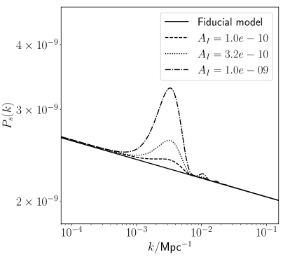
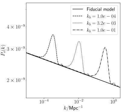
Figure 1: Left: Primordial power spectra for single bump models for different $A_{\rm I}$ values, $k_{b}$ fixed at $1.0\times 10^{-3}$ Mpc^-1; Right: single bump models for different $k_{b}$ values (the peaks occur at $3.35\times k_{b}$), $A_{\rm I}$ set at $1.0\times 10^{-9}$. The primordial power spectra for the fiducial model is plotted in solid line.

3 Methodology

We work in the framework of Friedmann-Lemaître-Robertson-Walker cosmology with a flat spatial geometry. The $\Lambda$CDM model is parametrized by the baryon density $\omega_{b}=\Omega_{b}h^{2}$, the cold dark matter density $\omega_{\text{cdm}}=\Omega_{\text{cdm}}h^{2}$, the present Hubble parameter $H_{0}$, and the optical depth to reionization, $\tau$.

Below, we briefly explain how we carry out the Bayesian analysis, the data products, and the codes used for the analysis.

3.1 Model selection

Let $M_{0}$ be the fiducial model with six parameters, and $M_{1}$ be the model that predicts primordial features with $n$ additional parameters (in this work, $n=2$ for the single bump model and $3$ for the multi-bump model). We compare the two models, $M_{0}$ and $M_{1}$, by the difference in their log-likelihood at best-fit values. Then, the quantity effective $\Delta\chi^{2}$ is given by [36, 37, 8]:

$$\Delta\chi^{2}_{\rm eff}:=\chi^{2}_{M_{1}}-\chi^{2}_{M_{0}}\,.$$ (3.1)

A negative value of $\Delta\chi^{2}_{\rm eff}$ quantifies the improvement in the fit due to the addition of parameters. For model comparison with $\geq 2$ degrees of freedom, $|\Delta\chi^{2}_{\rm eff}|<1$ may be considered a negligible improvement in the fit [38].

Bayesian analysis

In the Bayesian interpretation, probability measures a degree of belief. The Probability Distribution Function (PDF) of the model parameters after obtaining the data $d$, i.e., posterior probability, can be calculated using the Bayes theorem:

$$p(\theta|d)=\frac{p(\theta)\,p(d|\theta)}{p(d)}\,,$$ (3.2)

where $p(\theta)$ is the prior probability of parameter $\theta$, likelihood function $p(d|\theta)$ encloses experimental measurements, and $p(d)=\int p(d|\theta)\,p(\theta)\,d\theta=\mathcal{Z}$ is called the marginalized PDF of $d$, or Bayesian evidence.

Calculation of evidence for a model plays a prime role in the Bayesian model comparison. The ratio of evidences of two competing models, $M_{1}$ and $M_{0}$, is called the Bayes factor:

$$\mathcal{B}=\frac{\mathcal{Z}_{M_{1}}}{\mathcal{Z}_{M_{0}}}\,.$$ (3.3)

Interpretation of Bayes factor was given by Jeffreys’ scale [39, 40] using the quantity $\ln\mathcal{B}$, and shown in table 1 for reference. Negative values of $\ln\mathcal{B}$ mean preference of model $M_{0}$ with respect to model $M_{1}$.

$\mathbf{\ln\mathcal{B}}$	Preference of $M_{1}$ with respect to $M_{0}$
0 - 1	inconclusive
1 - 2.5	weak
2.5 - 5	moderate
$>~{}5$	strong

Table 1: Jeffreys’ scale [39] for Bayesian model comparison, interpretations modified by [40].

Data: We use a combination of the following data, in the form of the angular power spectrum $C_{\ell}$, from the Planck 2018 data release [41] (i) temperature and polarization data covering multipoles $\ell\sim 30$ to $\ell\sim 2500$ (TE and EE covering up to $\ell\sim 1996$); to avoid the exploration of the high-$\ell$ nuisance parameters, we use compressed and faster likelihood Plik_Lite, which includes marginalization over foregrounds and residual systematics. (ii) low $\ell$ polarization data (lowE) covering $\ell=2-29$, Plik-EE, (iii) low $\ell$ temperature data covering $\ell=2-29$, Plik-TT.
Codes: We use the Boltzmann code CLASS (The Cosmic Linear Anisotropy Solving System [42, 43]) to calculate the angular power spectrum of the CMB anisotropies for a cosmological model. To sample the parameter space, we use MontePython [44, 45], which is a publicly available Markov Chain Monte Carlo (MCMC) sampling package in Python. We use the nested sampling approach [46], which calculates the Bayesian evidence for a model. Nested sampling was incorporated in MontePython by the sampling method MultiNest [47, 48]. The triangle plots are generated with the package GetDist[49].

3.2 Selection of priors

The selection of prior probability is an essential ingredient in Bayesian statistics and reflects our initial knowledge about the model’s parameters. Our selection of prior ranges of cosmological parameters is given in table 2. The ranges of values of the fiducial model parameters are taken to be a few times the Planck $1\sigma$ values as provided in the recommended parameter file by MontePython for multinest sampling. We choose uniform probability distribution for the prior ranges of all the parameters. The priors for the analysis of single bump models are selected by taking different ranges of $\log k_{b}$ values. The justification for the different choices will be explained in the next section.

Model		Parameters	Prior ranges
Common parameters for		$100~{}\Omega_{b}$	[1.8, 3]
and all other models		$\Omega_{\text{cdm}}$	[0.1, 0.2]
fiducial model		$h$	[0.6, 0.8]
		$\tau_{\text{reio}}$	[0.004, 0.12]
		$\ln 10^{10}A_{s}$	[2.8904, 3.4012]
		$n_{s}$	[0.9, 1.1]
Single bump models	Prior-A	$\log A_{\rm I}$	[$-13$, $-8$]
		$\log k_{b}$	[$-4.5$, $-1.0$]
	Prior-B	$\log A_{\rm I}$	[$-13$, $-8$]
		$\log k_{b}$	[$-4.5$, $-2.2$]
	Prior-C	$\log A_{\rm I}$	[$-13$, $-8$]
		$\log k_{b}$	[$-2.2$, $-1.0$]
	Prior-D	$\log A_{\rm I}$	[$-13$, $-8$]
		$\log k_{b}$	[$-3.2$, $-2$]
Multi-bump model		$\log A_{\rm I}$	[$-13$, $-8$]
		$\log k_{1}$	[$-4.5$, $-1.0$]
		$\Delta$	[$0$, $1$]

Table 2: The selection of prior ranges for the cosmological parameters of fiducial, single bump, and multi-bump models.

4 Results

This section presents our results for the single bump and multi-bump models of particle production during inflation.

4.1 Single burst of particle production

We first carried out Bayesian analysis for the fiducial model with six parameters:
$~{}\Omega_{b},~{}\Omega_{cdm}$,$~{}h,~{}\tau,$ $~{}\ln 10^{10}A_{s},~{}n_{s}$, with the power spectrum given by eq. (2.10). We then incorporate a single bump using the power spectrum given by eq. (2.18) in CLASS, corresponding to a single burst of particle production during inflation and observable in CMB. This model has two additional parameters. Since the parameter $A_{\rm I}$ controls the amplitude of the bump, the upper limit of its prior range is chosen so that the posterior probability becomes negligible well within the prior range. The lower bound on $A_{\rm I}$ can be derived from the lower bound on model parameter $g$ using eq. (2.12). The theoretically estimated lower bound given in [31] is $g^{2}\gg 10^{-7}$, which gives $A_{\rm I}>10^{-17}$. The increment to the CMB power spectrum due to a bump with such a small amplitude is of $\mathcal{O}(10^{-9})$, which is indistinguishable from the fiducial model. Therefore, we choose the lower bound on $A_{\rm I}$ to be $10^{-13}$, which contributes an $\mathcal{O}(10^{-5})$ increment in the CMB power spectrum.

Next, the parameter $k_{b}$ that controls the bump’s location is not restricted from the theoretical model. In order to first understand its effect, we examine how varying $k_{b}$ affects the CMB power spectra, $\mathcal{D}^{XX}_{\ell}\equiv\ell(\ell+1)C^{XX}_{\ell}/2\pi$, where $XX$ stands for either $TT$, $TE$ or $EE$. We obtain the residual $\Delta\mathcal{D}^{XX}_{\ell}$ as

$$\Delta\mathcal{D}^{XX}_{\ell}\equiv\Delta\mathcal{D}^{XX,{\rm bump}}_{\ell}-\Delta\mathcal{D}^{XX,{\rm fid}}_{\ell},$$ (4.1)

where the superscripts ‘bump’ and ‘fid’ denote the bump and fiducial models, respectively.

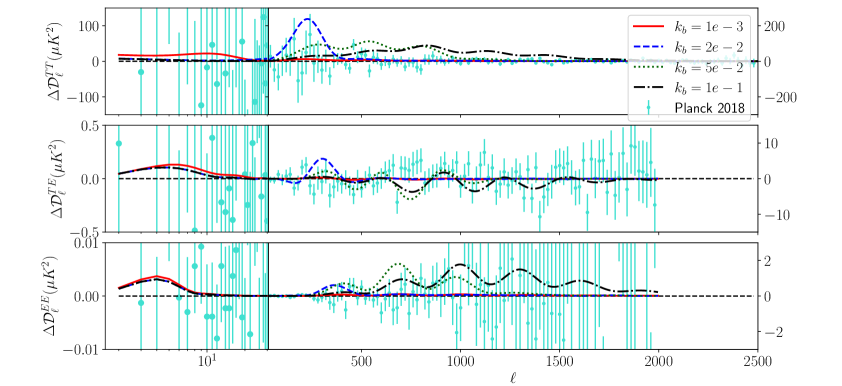
Figure 2: The residual CMB power spectra of single bump models with respect to the fiducial model, defined by eq. (4.1), for different values of $k_{b}$ and fixed $A_{\rm I}$. The three panels show CMB TT (top), TE (middle) and EE (bottom) power spectra, respectively. The data points with error bars, shown in cyan, are obtained by subtracting the fiducial model from the observed CMB power spectrum (Planck 2018).

Figure 2 shows $\Delta\mathcal{D}^{XX}_{\ell}$ for four different $k_{b}$ values, keeping $A_{\rm I}$ fixed to be $9\times 10^{-10}$ for all the cases. We find that $\Delta\mathcal{D}^{TT}_{\ell}$ is positive at all $\ell$. It exhibits oscillations which consist of one primary peak at some scale $\ell$ roughly set by $k_{b}$, followed by peaks of decreasing heights on either side of the primary peak. $\Delta\mathcal{D}^{TE}_{\ell}$ and $\Delta\mathcal{D}^{EE}_{\ell}$ also exhibit roughly similar oscillations. $\Delta\mathcal{D}^{TE}_{\ell}$ takes both positive and negative values, while $\Delta\mathcal{D}^{EE}_{\ell}$ is positive at all $\ell$. Interestingly, we see an additional rise of power at $\ell<10$ for TE and EE when a single bump is located at lower $k$ values. This can potentially lead to degeneracy with the optical depth to reionization, $\tau$. To examine this further, we compare the effect of the bump with the effect of varying $\tau$ in the angular power spectra. Figure 2 shows that incorporating primordial features at different $k_{b}$ affects the angular power spectrum at corresponding localized regions in $\ell$ space. It does not modify or shift the locations of the peaks of the oscillations. In comparison, varying $\tau$ introduces shifts of the peak locations, in addition to varying the height of the reionization bump for the polarization power spectrum at $\ell\leq 10$ (see figure 9 in appendix A for the CMB power spectra at different $\tau$). Therefore, the degeneracy with the optical depth is broken when data from all the multipoles are considered.

With the insight gained from the above study, we choose the following ranges of the prior for $k_{b}$:

• Prior-A: $-4.5<\log~{}k_{b}<-1.0$, a range of wave-numbers for $k_{b}$ such that the primordial bump-like features appear on all the multipole ranges constrained by Planck.

• Prior-B: $-4.5<\log~{}k_{b}<-2.2$, where the bump incorporated in the primordial power spectrum appears only in the lower multipole region of the CMB power spectrum.

• Prior C: $-2.2<\log~{}k_{b}<-1.0$, where the contribution of the bump is spread in the higher multipole region of the CMB TT power spectrum.

• Prior D: $-3.2<\log~{}k_{b}<-2.0$, a prior range in $k$-space such that the primordial bump-like features peak around the intermediate scale of CMB data, or the multipole region $\ell\sim(30,500)$.

We use flat prior probability distribution in log-space for both $A_{\rm I}$ and $k_{b}$. The results of our analysis are shown in table 3. The first column shows all the parameters of the fiducial and single bump models. The following columns show the best-fit values and $95\%$ limits of these parameters. A slight relative shift in the values of the cosmological parameters can be noticed in the table. The shifts for all the parameters are within the 1$\sigma$ uncertainty levels obtained from the Planck results. The last two rows are essential for model selection, as discussed in section 3.1. We provide the improvement in fitting due to individual likelihoods for all the models we consider in table 4. We also plot the best-fit power spectrum for different choices of priors in the top and middle panels of figure 3. The bottom panel shows corresponding CMB residual power spectra.

Parameters	Fiducial model		Single-bump model with different priors
			Prior-A		Prior-B		Prior-C		Prior-D
	Best-fit	$95\%$ limits	Best-fit	$95\%$ limits	Best-fit	$95\%$ limits	Best-fit	$95\%$ limits	Best-fit	$95\%$ limits
${100~{}\Omega_{b}}$	$2.237$	$2.236^{+0.030}_{-0.029}$	$2.239$	$2.236^{+0.029}_{-0.028}$	$2.235$	$2.236^{+0.028}_{-0.029}$	$2.231$	$2.236^{+0.029}_{-0.029}$	$2.233$	$2.234^{+0.030}_{-0.030}$
${\Omega_{cdm}}$	$0.1206$	$0.1203^{+0.0027}_{-0.0027}$	$0.1204$	$0.1202^{+0.0027}_{-0.0026}$	$0.1202$	$0.1203^{+0.0027}_{-0.0027}$	$0.1211$	$0.1203^{+0.0027}_{-0.0026}$	$0.1213$	$0.1202^{+0.0027}_{-0.0027}$
${h}$	$0.6716$	$0.673^{+0.012}_{-0.012}$	$0.6724$	$0.673^{+0.012}_{-0.012}$	$0.6731$	$0.673^{+0.012}_{-0.012}$	$0.6692$	$0.673^{+0.012}_{-0.012}$	$0.6688$	$0.673^{+0.012}_{-0.012}$
${\tau}$	$0.05357$	$0.055^{+0.016}_{-0.015}$	$0.05127$	$0.055^{+0.015}_{-0.015}$	$0.05438$	$0.055^{+0.016}_{-0.015}$	$0.05287$	$0.055^{+0.016}_{-0.015}$	$0.05265$	$0.055^{+0.016}_{-0.015}$
${\ln 10^{10}A_{s}}$	$3.044$	$3.046^{+0.033}_{-0.031}$	$3.039$	$3.046^{+0.032}_{-0.031}$	$3.046$	$3.046^{+0.032}_{-0.031}$	$3.043$	$3.045^{+0.033}_{-0.031}$	$3.048$	$3.045^{+0.033}_{-0.031}$
${n_{s}}$	$0.9641$	$0.9653^{+0.0086}_{-0.0084}$	$0.9678$	$0.9655^{+0.0089}_{-0.0087}$	$0.9650$	$0.9654^{+0.0086}_{-0.0083}$	$0.9678$	$0.9653^{+0.0086}_{-0.0092}$	$0.9669$	$0.9654^{+0.0090}_{-0.0089}$
$\log~{}{A_{\rm I}}$	$-$	$-$	$-10.73$	$-11.4^{+2.1}_{-1.6}$	$-11.04$	$-11.2^{+2.1}_{-1.8}$	$-10.74$	$-11.8^{+1.3}_{-1.2}$	$-10.57$	$-11.6^{+1.5}_{-1.4}$
$\log~{}k_{b}$	$-$	$-$	$-2.07$	$-3.0^{+1.9}_{-1.5}$	$-2.38$	$-3.48^{+1.1}_{-0.99}$	$-2.07$	$-1.64^{+0.56}_{-0.55}$	$-2.04$	$-2.59^{+0.59}_{-0.55}$
${\Delta\chi^{2}_{\rm eff}}$	$-$		$-0.29$		$-0.18$		$-0.96$		$-1.12$
${\ln\mathcal{B}}$	$-$		0.4		0.3		0.2		0.4

Table 3: Best-fit and $95\%$ limits of parameters for the fiducial model and the single-bump model for different choices of the prior range. $\Delta\chi^{2}_{\rm eff}$ and the Bayes factor $\ln\mathcal{B}$ are quoted in the last two rows.

Model		$\mathbf{\Delta\chi^{2}_{\rm eff}}$
		TTTEEE (high $\ell$)	TT (low $\ell$)	EE (low $\ell$)	Total
	Prior-A	$1.06$	$-1.04$	$-0.30$	$-0.29$
Single bump	Prior-B	$-0.13$	$-0.16$	$0.10$	$-0.18$
models	Prior-C	$0.16$	$-0.96$	$-0.16$	$-0.96$
	Prior-D	$-0.58$	$-0.73$	$0.19$	$-1.12$
Multi-bump model		$-2.22$	$-1.40$	$0.55$	$-3.07$

Table 4: $\Delta\chi^{2}_{\rm eff}$ of the single bump and multi-bump models calculated for individual likelihoods.

The best-fit values and $95\%$ limits of all the parameters obtained from the Bayesian analysis with Prior-A are given in the fourth and fifth columns of table 3. We notice that the value of $\chi^{2}$ has not changed much by adding two more parameters. Referring to Jeffrey’s scale in table 1, the Bayes factor $|\ln\mathcal{B}|<1$ indicates an inconclusive preference toward the models under consideration. The one and two-dimensional marginalized posterior distributions of the power spectrum parameters for Prior-A are shown on the top-left side of figure 4.

The best-fit values and $95\%$ limits of the parameters for the single bump model with Prior-B (primordial features appearing at the lower $\ell$ of the CMB power spectrum) are given in the sixth and seventh columns of table 3. No significant change in $\chi^{2}$ value was noticed due to the primordial feature in this region. The value of the Bayes factor is $|\ln\mathcal{B}|<1$ implies an inconclusive preference of models under consideration. The one and two-dimensional marginalized posterior distributions of the power spectrum parameters for Prior-B are shown on the top-right side of figure 4.

Next, we estimate the maximum amplitude of primordial features that the CMB low-$\ell$ data may accommodate. The $95\%$ Confidence Level (CL) upper limit on $A_{\rm I}$ obtained from one-dimensional marginalized posterior distribution is $\sim 7\times 10^{-10}$, or about $35\%$ of the amplitude of scalar perturbations in the fiducial model, $A_{s}$. The amplitude of the observable features helps to put a constraint on one of the theoretical model parameters. From eq. (2.12), we found an upper limit on the dimensionless coupling constant, $g$, in the region chosen for Prior-B:

$$g<0.1\,.$$ (4.2)

This constraint on the parameter $g$ leaves a large region of natural values.

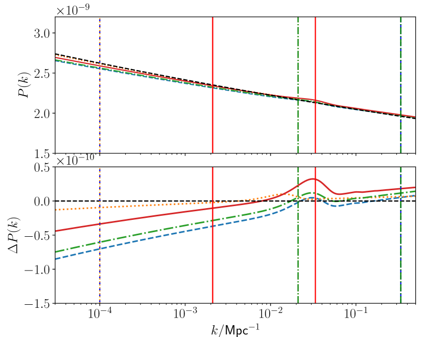
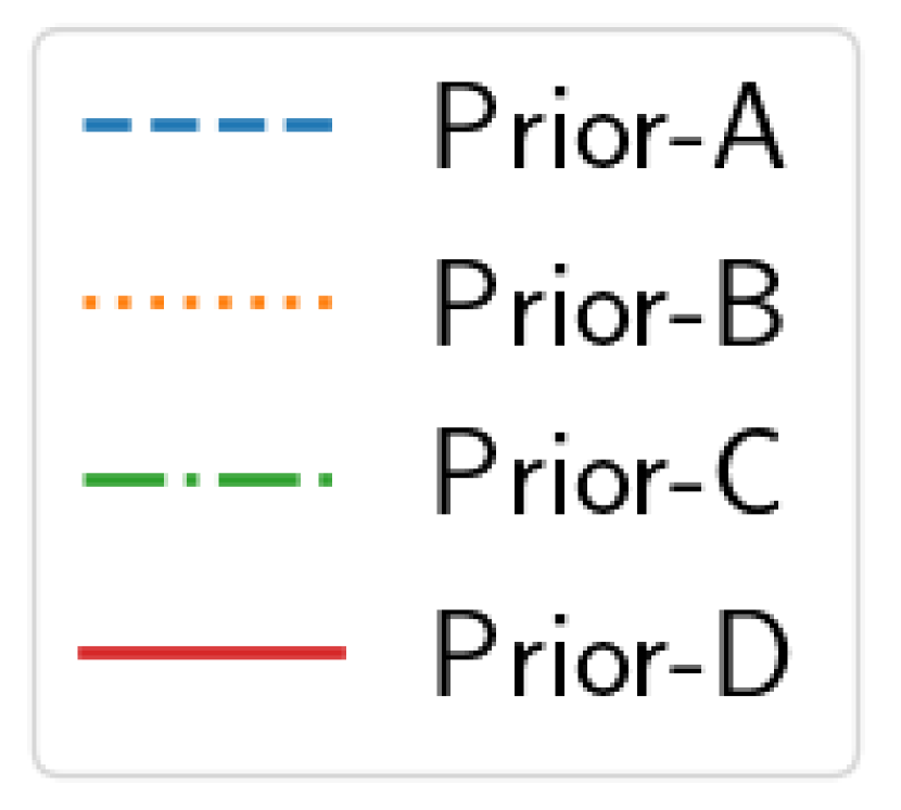
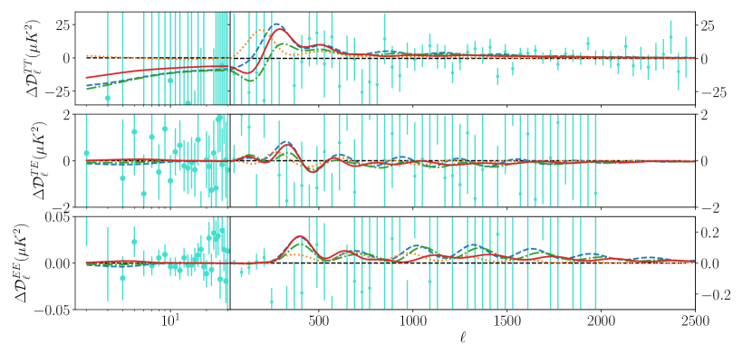
Figure 3: Top: The primordial power spectrum corresponding to best-fit parameters of the single bump models. Middle: Same as the top but difference in the power spectrum, $\Delta P(k):=P_{\rm bump}(k)-P_{\rm fiducial}(k)$, on the vertical axis. The peaks of the bumps are at $k_{p}\simeq 3.35~{}k_{b}$. The vertical lines mark our choices of prior range in terms of $k_{p}$. Bottom: The residuals in CMB TT, TE, and EE power spectra of best-fit single bump models with respect to the fiducial model. The data points with error bars are obtained by subtracting the fiducial model from the observed CMB power spectrum by Planck 2018.

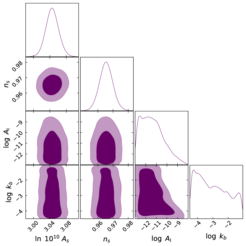
(a) Prior-A

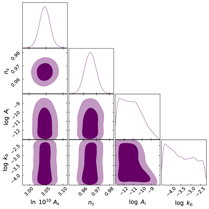
(b) Prior-B

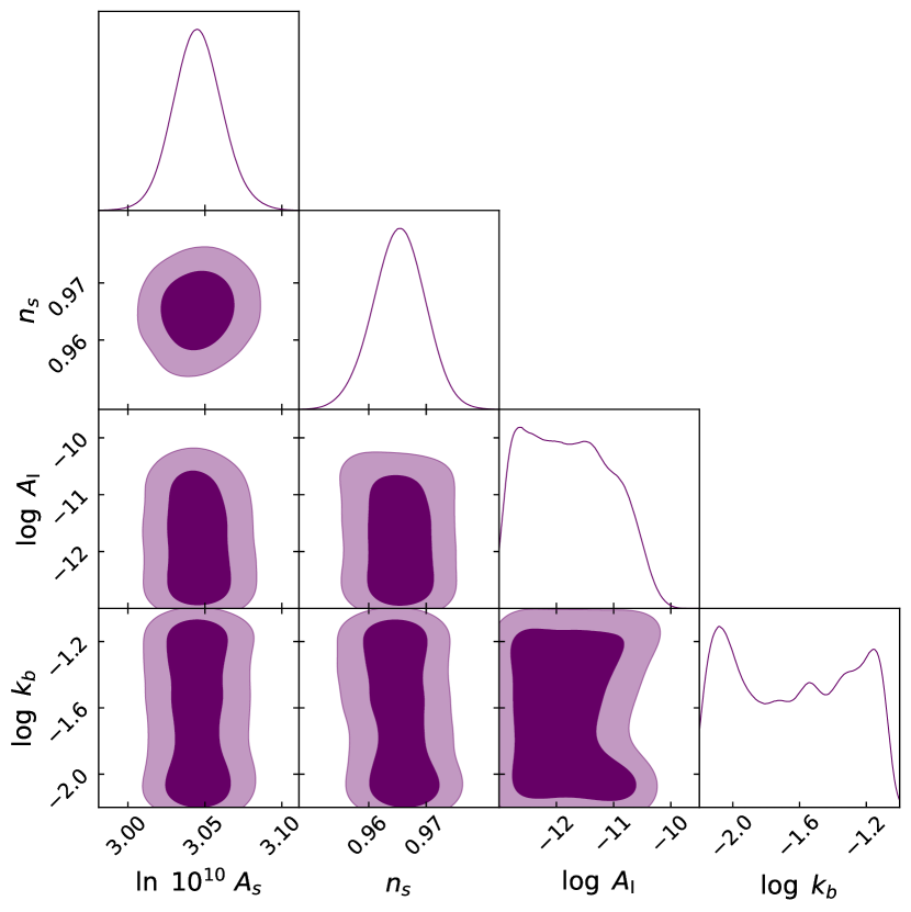
(c) Prior-C

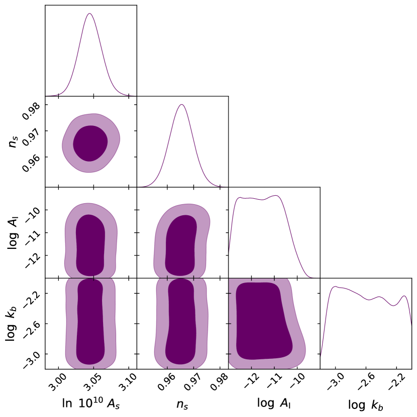
(d) Prior-D

Figure 4: The one and two-dimensional posterior distributions of the parameters for the single bump model corresponding to the power spectrum eq. (2.18) for different choices of prior. The light and dark shaded regions indicate parameter space corresponding to 68% and 95% confidence levels, respectively.

The search for bump-like features on the higher multipoles of the CMB data with Prior-C gives best-fit values and $95\%$ limits, as quoted in the eighth and ninth columns of table 3. The best-fit feature is located around $9\times 10^{-3}\text{Mpc}^{-1}$, giving an improved $\Delta\chi^{2}_{\rm eff}\sim-1$. From table 4, it can be seen that the low-$\ell$ temperature data contributes more to improve the fitting. The value of the Bayes factor again indicates an inconclusive preference for models with available data. The one and two-dimensional marginalized posterior distributions of the power spectrum parameters are shown on the bottom-left side of figure 4. From one dimensional marginalized PDF, the upper bound ($95\%$ CL) on $A_{\rm I}$ was found to be $\sim 3\times 10^{-11}$, or $1.5\%A_{s}$. From eq. (2.12), we found that

$$g<6\times 10^{-2}\,.$$ (4.3)

Investigation of localized features: To avoid the multipole region where the primordial features are spread out, next, we carry out Bayesian analysis with Prior-D. Results of the analysis with Prior-D are given in the last two columns of table 3. Interestingly, we find that the best-fit value of the parameter $k_{b}$ points closer to the one obtained in cases of Prior-A and C, giving a slight improvement in the $\chi^{2}$ value. The corresponding primordial power spectrum and CMB residual power spectrum in figure 3 may help the reader visualize the same. The one and two-dimensional marginalized posterior distributions of the power spectrum parameters are shown on the bottom-right side of figure 4. The $95\%$ CL upper limit on $A_{\rm I}$ was found to be $\sim 8\times 10^{-11}$, or $4\%A_{s}$. From eq. (2.12), we found that

$$g<8\times 10^{-2}\,.$$ (4.4)

With the motivation to explain a slight excess in the CMB residual power spectra, we have also carried out Bayesian analyses of single bump models with narrow prior ranges and uniform probability distribution in $k_{b}$. Including a narrow prior in $k_{b}$ that incorporates features near $\ell:200-500$, we obtained $\Delta\chi^{2}_{\rm eff}=-1.1$ with the best-fit value $k_{b}$ same as Priors A, C and D, confirming our previous results. Bayesian analysis of another narrow prior in $k_{b}$ that incorporates features near $\ell:10-20$ showed a negligible improvement in the fit. We observed no significant improvement in the Bayes factor values for both cases.

We remark that our results of the single bump models show prior dependence as the different prior ranges of $k_{b}$ search for features on different angular scales of the CMB data. We also note that the parameter $k_{b}$ is not constrained for any of the analysed models, as shown in figure 4. However, the analyses with multiple prior choices prefer a single bump at almost the same location (see figure 3). We also obtain upper bounds on the amplitudes of primordial features predicted from particle physics models of inflation on different scales probed by the Planck.

4.2 Multiple bursts of particle production

As explained in section 2, multiple bursts of particle production during inflation may produce multiple bump-like features on the primordial power spectrum [28, 31, 27, 26]. The location of the $i$-th bump is parameterized by $k_{i}=e^{(i-1)\Delta}k_{1}$, where $k_{1}$ specifies the location of the first bump via eq. (2.17) while $\Delta$ controlling the spacing between subsequent bumps. Here, we take $\Delta$ to be constant, as its $\phi$-dependence does not significantly change the qualitative feature of the power spectrum in the parameter region we will consider. Therefore, we have three additional parameters in the multi-bump model compared to the fiducial model: $A_{\rm I}$, $k_{1}$, and $\Delta$.

We choose the same prior range for the parameter $A_{\rm I}$ as the single bump model. We need to specify the prior ranges for $k_{1}$ and $\Delta$. The number of bumps could be large enough to cover the whole observable range. We consider a phenomenological model in which the first episode of a burst of particle production can occur at any scale $k_{1}$, followed by a series of bumps over the scales $k>k_{1}$. Therefore, we allow the prior range of $k_{1}$ to be as broad as the observable scale of Planck. Next, we need to specify a prior range for $\Delta$. Note that if the features are widely spaced, we expect that the constraints on each bump will be similar to that of single bump models. When $0\leq\Delta\leq 1$, the multi-bumps on the primordial power spectrum largely overlap. In what follows, we present the result of Bayesian analysis for the multi-bump model for this choice of the prior range of $\Delta$ and describe how it compares with the fiducial model.

Parameters	Multi-bump model
	Best-fit	$95\%$ limits
$100\Omega_{b}$	$2.235$	$2.236^{+0.028}_{-0.028}$
$\Omega_{\text{cdm}}$	$0.121$	$0.1202^{+0.0027}_{-0.0026}$
$h$	$0.6704$	$0.673^{+0.011}_{-0.012}$
$\tau_{\text{reio}}$	$0.05751$	$0.055^{+0.016}_{-0.015}$
$\ln 10^{10}A_{s}$	$3.015$	$3.042^{+0.032}_{-0.034}$
$n_{s}$	$0.9644$	$0.9650^{+0.0083}_{-0.0086}$
$\log~{}A_{\rm I}$	$-10.27$	$-11.9^{+1.3}_{-1.1}$
$\log~{}k_{1}$	$-2.74$	$-2.8^{+1.6}_{-1.6}$
$\Delta$	$0.799$	$0.57^{+0.42}_{-0.47}$
$\Delta\chi^{2}_{\rm eff}$	$-3.07$
$\ln\mathcal{B}$	$0.8$

Table 5: Best-fit and $95\%$ limits of the parameters of the multi-bump model with prior $0~{}\leq~{}\Delta~{}\leq~{}1$.

The best-fit values and $95\%$ limits obtained from the Bayesian analysis of the multi-bump model are given in table 5. The primordial power spectrum in eq. (2.11) corresponding to best-fit values of the parameters is shown by the solid blue curve in figure 5. For comparison, the power-law form for the fiducial model is also shown (dashed red curve). The best-fit multi-bump model corresponds to the particle production mechanism commencing at $k_{1}\simeq 1.8\times 10^{-3}$ Mpc^-1 and continuing at the higher $k$ - scales.

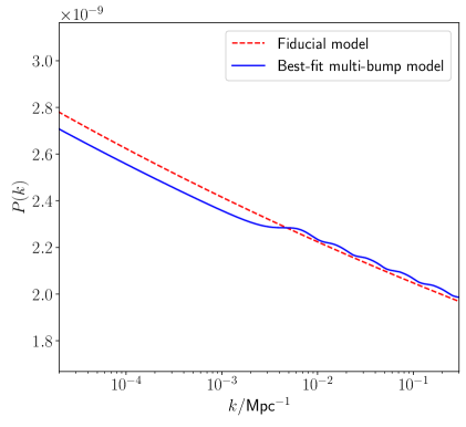
Figure 5: The primordial power spectrum corresponding to best-fit values of the multi-bump model.

The 1D and 2D marginalized posterior distributions for the power spectrum parameters are shown in figure 6.

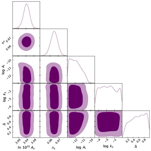
Figure 6: The 1D and 2D marginalized posterior distributions for the parameters of the multi-bump model.

The last two rows of table 5 show that the difference in maximum log-likelihood values between the fiducial and the multi-bump models is ${\Delta\chi^{2}_{\rm eff}\sim-3}$. Table 4 shows that the maximum contribution to the improvement in fitting comes from temperature data. The Bayes factor obtained for the case of the multi-bump model is ${\ln\mathcal{B}=0.8}$. Compared to the single bump models we have investigated so far, the multi-bump model gives a better improvement in the fit and the Bayes factor value.

We plot the residuals in CMB TT, TE and EE power spectra of the best-fit multi-bump model with respect to the fiducial model in figure 7. The data points with error bars are obtained after subtracting the best-fit fiducial model from the Planck 2018 data. The improvement in the statistical quantities for the multi-bump case seems to be the improvement in the fit in the lower multipole region of the CMB TT power spectrum, explaining the suppression in large-scale powers followed by oscillations at higher multipoles, which is also evident from the $\Delta\chi^{2}_{\rm eff}$ values in the last row of table 4.

Next, to determine the constraint on the theoretical model parameter $g$, we note that the $95\%$ CL upper bound on the amplitude of the multi-bump feature was $2.1\times 10^{-11}$, or $\sim 1\%$ of $A_{s}$. Therefore, using eq. (2.12), we find that

$$g<5\times 10^{-2}.$$ (4.5)

Eq. (4.5) is the tightest upper bound obtained in our analysis and still within the natural values (see footnote 9).

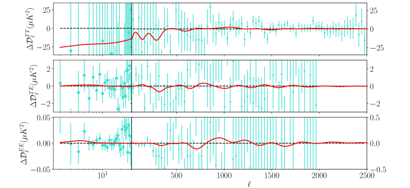
Figure 7: The residuals in CMB TT, TE, and EE power spectra of the best-fit multi-bump model with respect to the fiducial model. The data points with error bars are obtained by subtracting the fiducial model from the observed CMB power spectrum (Planck 2018).

For completeness of the analysis, we have also carried out the Bayesian analysis of multi-bump models with the following prior ranges: (i) $0\leq\Delta\leq 3$: we obtained $\Delta\chi^{2}_{\rm eff}$ value of $-0.3$ and Bayes factor $0.6$ for this prior range, (ii) $0\leq\Delta\leq 0.5$: we obtained $\Delta\chi^{2}_{\rm eff}$ value of $-1.0$ and Bayes factor $0.7$ for this case. The upper bound on model parameter $g$ was consistent with eq. (4.5) in both the cases. We do not discuss these cases further since they do not provide significantly better fits of the models to the data compared with the fiducial model.

5 Summary and Discussions

In this work, we investigated the imprints of a class of models involving particle productions during inflation [33, 34, 35] using the latest CMB data from Planck. This class of models predicts bump-like features in the primordial power spectrum whenever bursts of particle production occur during inflation. We parametrize the primordial power spectrum using the analytical expression for the bump-like features, including dominant and subdominant contributions calculated in [31]. We have carried out Bayesian analyses to constrain one of the parameters of the theoretical model.

We summarize our results below for single burst of particle production in the following three regimes of angular scales of CMB data.

• Features in the large-scale (low-$\ell$) CMB data: The Bayesian analysis for the search of features on larger scales, i.e., prior-B ($-4.5<\log~{}k_{b}<-2.2$), returned a minor change in the $\chi^{2}$ value. The limit on the model parameter responsible for particle production was $g<0.1$. The 1D marginalized posterior distribution shows that multipole $\ell\lesssim 500$ in CMB data may accommodate primordial features of this kind with amplitude as large as $\sim 35\%A_{s}$ ($95\%$ CL).

• Features in the small-scale (high-$\ell$) CMB data: We found a marginal improvement in the $\chi^{2}$ value ($\Delta\chi^{2}_{\rm eff}\sim 1$) when the position of the bump was confined in the small-scale region, i.e., prior-C ($-2.2<\log~{}k_{b}<-1.0$). The constraint on the model parameter is relatively tighter in the small-scale region: $g<0.06$. The 1D marginalized posterior distribution shows that the higher multipole CMB data may accommodate primordial features with a smaller amplitude, i.e., $1.5\%A_{s}$ ($95\%$ CL).

• Features in the intermediate scale CMB data: We observed again a slight improvement in the fitting with prior $k_{b}$ having intermediate scales, i.e., prior-D ($-3.2<\log~{}k_{b}<-2.0$). The $95\%$ CL upper limit on $A_{\rm I}$ was found to be $4\%A_{s}$. In this case, the upper bound on the model parameter was $g<0.08$.

We note that the Bayes factors $\ln\mathcal{B}$ for all the single bump models are positive yet within the inconclusive range as per Jeffreys’ scale (table 1). Though we could not constrain the parameter $k_{b}$, our analysis with multiple prior ranges points towards nearly the same best-fit location of the single bump (see figure  3).

The results for multiple bursts of particle production during inflation are summarized as follows: We found a better fit to the data in the case of multi-bump model when the parameter $\Delta$ that specifies the distance between the subsequent bumps was confined between $0$ and $1$, which corresponds to largely overlapping multiple bumps. The 1D marginalized posterior distribution returned a $95\%$ CL upper limit on $A_{\rm I}$, i.e., $\sim 1\%A_{s}$. In this case, we obtained the tightest upper bound on the model parameter, $g<0.05$. The improvement in $\Delta\chi^{2}_{\rm eff}$ was about $-3$ due to the better fit at low multipoles followed by bumps at higher multipoles. The Bayes factor was 0.8, the highest one obtained in our analysis. Though the result does not indicate strong evidence for the presence of features due to particle production during inflation, it is interesting to note that the imprints of a multi-bump model are still compatible with the Planck 2018 data. Using Bayesian evidence and interpretations given by Jeffreys’ scale (table 1), we conclude that the presence or absence of bump-like primordial features is inconclusive from the available Planck 2018 data. However, we found $95\%$ CL upper limits on the amplitudes of the primordial features $A_{\rm I}$ at different scales, which is important for obtaining the upper bound on one of the theoretical model parameters $g$ responsible for the particle production.

The range of co-moving wave-numbers over which the temperature power spectrum is sensitive for primordial features, $0.0002\lesssim k/\text{Mpc}^{-1}\lesssim 0.15$, has been covered at the cosmic variance limit by Planck [7]. The multipole range $\ell>2000$ in the temperature power spectrum, where experimental noise dominates the cosmic variance, is less sensitive to the study of features as the CMB temperature signal becomes subdominant in this region [30]. However, the E-component polarization acts as a complementary dataset for searching for features in the primordial power spectrum. Though Planck’s polarization data provides valuable information at intermediate scales, it is not limited by the cosmic variance for small angular scales. Future experiments aimed at measuring CMB polarization with improved sensitivity and broad coverage of angular scales are expected to provide tighter constraints on the inflation models.

Primordial features arising from particle production during inflation are expected to leave imprints on primordial non-Gaussianity (see, e.g. [29]). We do not include a discussion of non-Gaussianity here and postpone the investigation to future work. We also do not discuss tensor perturbations in this paper since the effect of particle productions on the tensor power spectrum is expected to be small [53, 54, 55, 56, 31]. Any feature in the primordial power spectrum should also be encoded in other cosmological observables besides the CMB. Following this rationale, there have been substantial efforts to search for the signatures of primordial features in futuristic large-scale structure surveys [57, 58, 59, 60, 61, 62] and stochastic gravitational background waves [63, 64]. Moreover, upcoming redshifted 21 cm surveys can help explore the features in the primordial power spectrum on scales inaccessible to other probes of matter distributions. Recent studies have shown that future 21 cm surveys can improve the constraints on inflationary features by a few orders of magnitude [65, 66]. We plan to address possible constraints on particle production during inflation from future redshifted 21 cm observations in the forthcoming work.

Appendix A Potential degeneracy between the location of bump-like features and optical depth to reionization

In this section, we investigate the improvement in the fitting for the best-fit multi-bump model (table 5) due to changes in cosmological parameters and the addition of multi-bumps separately. In figure 8, we plot the CMB residual power spectra corresponding to (i) best-fit multi-bump model (solid red), (ii) contribution coming only due to the addition of multi-bumps - cosmological parameters are fixed to that of the fiducial model (dashed blue), and (iii) contribution coming only due to a shift in the cosmological parameters, from the fiducial model without including the multi-bumps (dotted black). We note the following:

1. Lower multipole region:

   • TT power spectrum - The suppression of powers for the best-fit multi-bump model is majorly due to the shift in the cosmological parameters compared with the best-fit fiducial model.

   • TE and EE power spectra - The contribution to the power spectrum due to the multi-bumps in this region is negligible, and a change in cosmological parameters contributes to the excess of powers.

2. Higher multipole region: The multi-bumps start at higher $k$ on the best-fit multi-bump power spectrum, which is reflected as the excess of powers in TT and EE power spectra. The change in cosmological parameters causes suppression of powers. Therefore, the observed improvement in the fitting in this region is the combined effect of both.

Next, as an example, we present the effect of variations in one of the cosmological parameters, optical depth to reionization, $\tau$. We plot the CMB residual power spectra of TT, TE and EE correlations for different values of $\tau$ in figure 9. The power spectra are produced by fixing the cosmological parameters to the Planck best-fit value except for $\tau$ and subtracting from them, the Planck best-fit model with $\tau_{\rm Planck}=0.0543$. Varying the optical depth introduces a shift of the peak locations, in addition to varying the height of the reionization bump for the polarization power spectrum at $\ell\leq 10$. The excess (lack) of powers in TE and EE panels at low $\ell$ is produced when $\tau>\tau_{\rm Planck}$ ($<\tau_{\rm Planck}$). The variation in other cosmological parameters can shift acoustic peaks, stretch the spectrum or modulate the heights of the peaks [69].

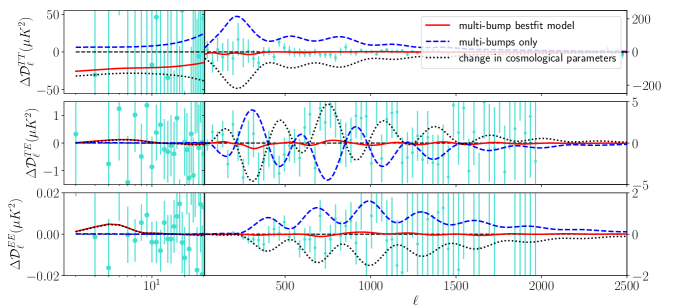
Figure 8: The residual CMB power spectra for (i) best-fit multi-bump model (solid red), (ii) multi-bumps with cosmological parameters fixed to that of the fiducial model (dashed blue), and (iii) changes in cosmological parameters without including the multi-bumps (dotted black).

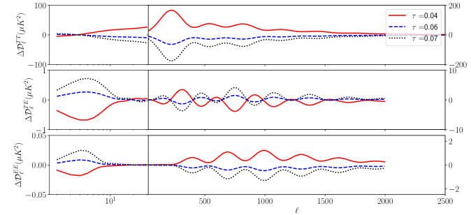
Figure 9: The residual CMB power spectra obtained by subtracting the Planck best-fit model from models with different values of optical depth to reionization, $\tau$. All other cosmological parameters are fixed.

References

- [1] A.H. Guth, Inflationary universe: A possible solution to the horizon and flatness problems, Phys. Rev. D 23 (1981) 347.
- [2] A. Linde, A new inflationary universe scenario: A possible solution of the horizon, flatness, homogeneity, isotropy and primordial monopole problems, Physics Letters B 108 (1982) 389.
- [3] A. Albrecht and P.J. Steinhardt, Cosmology for grand unified theories with radiatively induced symmetry breaking, Phys. Rev. Lett. 48 (1982) 1220.
- [4] A. Starobinsky, A new type of isotropic cosmological models without singularity, Physics Letters B 91 (1980) 99.
- [5] K. Sato, First-order phase transition of a vacuum and the expansion of the Universe, Monthly Notices of the Royal Astronomical Society 195 (1981) 467 [https://academic.oup.com/mnras/article-pdf/195/3/467/4065201/mnras195-0467.pdf].
- [6] D. Kazanas, Dynamics of the universe and spontaneous symmetry breaking, ApJ 241 (1980) L59.
- [7] Planck collaboration, Planck 2018 results. I. Overview and the cosmological legacy of Planck, Astron. Astrophys. 641 (2020) A1 [1807.06205].
- [8] Planck collaboration, Planck 2018 results. X. Constraints on inflation, Astron. Astrophys. 641 (2020) A10 [1807.06211].
- [9] E. Silverstein and A. Westphal, Monodromy in the CMB: Gravity Waves and String Inflation, Phys. Rev. D 78 (2008) 106003 [0803.3085].
- [10] R. Flauger, L. McAllister, E. Pajer, A. Westphal and G. Xu, Oscillations in the CMB from Axion Monodromy Inflation, JCAP 06 (2010) 009 [0907.2916].
- [11] J.A. Adams, B. Cresswell and R. Easther, Inflationary perturbations from a potential with a step, Phys. Rev. D 64 (2001) 123514 [astro-ph/0102236].
- [12] X. Chen, R. Easther and E.A. Lim, Large Non-Gaussianities in Single Field Inflation, JCAP 06 (2007) 023 [astro-ph/0611645].
- [13] A. Achucarro, J.-O. Gong, S. Hardeman, G.A. Palma and S.P. Patil, Features of heavy physics in the CMB power spectrum, JCAP 01 (2011) 030 [1010.3693].
- [14] V. Miranda, W. Hu and P. Adshead, Warp Features in DBI Inflation, Phys. Rev. D 86 (2012) 063529 [1207.2186].
- [15] N. Bartolo, D. Cannone and S. Matarrese, The Effective Field Theory of Inflation Models with Sharp Features, JCAP 10 (2013) 038 [1307.3483].
- [16] D.K. Hazra, A. Shafieloo, G.F. Smoot and A.A. Starobinsky, Wiggly Whipped Inflation, JCAP 08 (2014) 048 [1405.2012].
- [17] R.K. Jain, P. Chingangbam, J.-O. Gong, L. Sriramkumar and T. Souradeep, Punctuated inflation and the low CMB multipoles, JCAP 01 (2009) 009 [0809.3915].
- [18] A.A. Starobinsky, Spectrum of adiabatic perturbations in the universe when there are singularities in the inflation potential, JETP Lett. 55 (1992) 489.
- [19] S. Cremonini, Z. Lalak and K. Turzynski, Strongly Coupled Perturbations in Two-Field Inflationary Models, JCAP 03 (2011) 016 [1010.3021].
- [20] M. Braglia, D.K. Hazra, L. Sriramkumar and F. Finelli, Generating primordial features at large scales in two field models of inflation, JCAP 08 (2020) 025 [2004.00672].
- [21] M. Braglia, D.K. Hazra, F. Finelli, G.F. Smoot, L. Sriramkumar and A.A. Starobinsky, Generating PBHs and small-scale GWs in two-field models of inflation, JCAP 08 (2020) 001 [2005.02895].
- [22] X. Chen, M.H. Namjoo and Y. Wang, Models of the Primordial Standard Clock, JCAP 02 (2015) 027 [1411.2349].
- [23] M. Braglia, X. Chen and D.K. Hazra, Comparing multi-field primordial feature models with the Planck data, JCAP 06 (2021) 005 [2103.03025].
- [24] M. Braglia, X. Chen and D.K. Hazra, Uncovering the History of Cosmic Inflation from Anomalies in Cosmic Microwave Background Spectra, 2106.07546.
- [25] M. Braglia, X. Chen and D.K. Hazra, Primordial Standard Clock Models and CMB Residual Anomalies, 2108.10110.
- [26] D.J.H. Chung, E.W. Kolb, A. Riotto and I.I. Tkachev, Probing Planckian physics: Resonant production of particles during inflation and features in the primordial power spectrum, Phys. Rev. D62 (2000) 043508 [hep-ph/9910437].
- [27] N. Barnaby, Z. Huang, L. Kofman and D. Pogosyan, Cosmological Fluctuations from Infra-Red Cascading During Inflation, Phys. Rev. D80 (2009) 043501 [0902.0615].
- [28] N. Barnaby and Z. Huang, Particle Production During Inflation: Observational Constraints and Signatures, Phys. Rev. D 80 (2009) 126018 [0909.0751].
- [29] N. Barnaby, On Features and Nongaussianity from Inflationary Particle Production, Phys. Rev. D 82 (2010) 106009 [1006.4615].
- [30] J. Chluba, J. Hamann and S.P. Patil, Features and New Physical Scales in Primordial Observables: Theory and Observation, Int. J. Mod. Phys. D 24 (2015) 1530023 [1505.01834].
- [31] L. Pearce, M. Peloso and L. Sorbo, Resonant particle production during inflation: a full analytical study, JCAP 1705 (2017) 054 [1702.07661].
- [32] M. Ballardini, F. Finelli, F. Marulli, L. Moscardini and A. Veropalumbo, New constraints on primordial features from the galaxy two-point correlation function, 2202.08819.
- [33] K. Furuuchi, Excursions through KK modes, JCAP 1607 (2016) 008 [1512.04684].
- [34] K. Furuuchi, S.S. Naik and N.J. Jobu, Large Field Excursions from Dimensional (De)construction, JCAP 06 (2020) 054 [2001.06518].
- [35] K. Furuuchi, N.J. Jobu and S.S. Naik, Extra-Natural Inflation (De)constructed, 2004.13755.
- [36] Planck collaboration, Planck 2013 results. XXII. Constraints on inflation, Astron. Astrophys. 571 (2014) A22 [1303.5082].
- [37] Planck collaboration, Planck 2015 results. XX. Constraints on inflation, Astron. Astrophys. 594 (2016) A20 [1502.02114].
- [38] W.H. Press, S.A. Teukolsky, W.T. Vetterling and B.P. Flannery, Numerical Recipes 3rd Edition: The Art of Scientific Computing, Cambridge University Press, 3 ed. (2007).
- [39] H. Jeffreys, The Theory of Probability, Oxford Classic Texts in the Physical Sciences (1939).
- [40] R. Trotta, Applications of Bayesian model selection to cosmological parameters, Mon. Not. Roy. Astron. Soc. 378 (2007) 72 [astro-ph/0504022].
- [41] Planck collaboration, Planck 2018 results. VI. Cosmological parameters, Astron. Astrophys. 641 (2020) A6 [1807.06209].
- [42] J. Lesgourgues, The Cosmic Linear Anisotropy Solving System (CLASS) I: Overview, 1104.2932.
- [43] D. Blas, J. Lesgourgues and T. Tram, The Cosmic Linear Anisotropy Solving System (CLASS). Part II: Approximation schemes, JCAP 2011 (2011) 034 [1104.2933].
- [44] T. Brinckmann and J. Lesgourgues, MontePython 3: boosted MCMC sampler and other features, 1804.07261.
- [45] B. Audren, J. Lesgourgues, K. Benabed and S. Prunet, Conservative Constraints on Early Cosmology: an illustration of the Monte Python cosmological parameter inference code, JCAP 1302 (2013) 001 [1210.7183].
- [46] J. Skilling, Nested sampling for general Bayesian computation, Bayesian Analysis 1 (2006) 833.
- [47] F. Feroz and M. Hobson, Multimodal nested sampling: an efficient and robust alternative to MCMC methods for astronomical data analysis, Mon. Not. Roy. Astron. Soc. 384 (2008) 449 [0704.3704].
- [48] F. Feroz, M. Hobson and M. Bridges, MultiNest: an efficient and robust Bayesian inference tool for cosmology and particle physics, Mon. Not. Roy. Astron. Soc. 398 (2009) 1601 [0809.3437].
- [49] A. Lewis, GetDist: a Python package for analysing Monte Carlo samples, 1910.13970.
- [50] G. ’t Hooft, Naturalness, chiral symmetry, and spontaneous chiral symmetry breaking, NATO Sci. Ser. B 59 (1980) 135.
- [51] K. Furuuchi and Y. Koyama, Large field inflation models from higher-dimensional gauge theories, JCAP 02 (2015) 031 [1407.1951].
- [52] W. Lee, K.-W. Ng, I.-C. Wang and C.-H. Wu, Trapping effects on inflation, Phys. Rev. D 84 (2011) 063527 [1101.4493].
- [53] N. Barnaby, J. Moxon, R. Namba, M. Peloso, G. Shiu and P. Zhou, Gravity waves and non-Gaussian features from particle production in a sector gravitationally coupled to the inflaton, Phys. Rev. D 86 (2012) 103508 [1206.6117].
- [54] D. Carney, W. Fischler, E.D. Kovetz, D. Lorshbough and S. Paban, Rapid field excursions and the inflationary tensor spectrum, JHEP 11 (2012) 042 [1209.3848].
- [55] J.L. Cook and L. Sorbo, Particle production during inflation and gravitational waves detectable by ground-based interferometers, Phys. Rev. D 85 (2012) 023534 [1109.0022].
- [56] L. Senatore, E. Silverstein and M. Zaldarriaga, New Sources of Gravitational Waves during Inflation, JCAP 08 (2014) 016 [1109.0542].
- [57] B. L’Huillier, A. Shafieloo, D.K. Hazra, G.F. Smoot and A.A. Starobinsky, Probing features in the primordial perturbation spectrum with large-scale structure data, Mon. Not. Roy. Astron. Soc. 477 (2018) 2503 [1710.10987].
- [58] T. Chantavat, C. Gordon and J. Silk, Large Scale Structure Forecast Constraints on Particle Production During Inflation, Phys. Rev. D 83 (2011) 103501 [1009.5858].
- [59] X. Chen, C. Dvorkin, Z. Huang, M.H. Namjoo and L. Verde, The Future of Primordial Features with Large-Scale Structure Surveys, JCAP 11 (2016) 014 [1605.09365].
- [60] M. Ballardini, F. Finelli, C. Fedeli and L. Moscardini, Probing primordial features with future galaxy surveys, JCAP 10 (2016) 041 [1606.03747].
- [61] G.A. Palma, D. Sapone and S. Sypsas, Constraints on inflation with LSS surveys: features in the primordial power spectrum, JCAP 06 (2018) 004 [1710.02570].
- [62] M. Ballardini, F. Finelli, R. Maartens and L. Moscardini, Probing primordial features with next-generation photometric and radio surveys, JCAP 04 (2018) 044 [1712.07425].
- [63] M. Braglia, X. Chen and D.K. Hazra, Probing Primordial Features with the Stochastic Gravitational Wave Background, JCAP 03 (2021) 005 [2012.05821].
- [64] J. Fumagalli, S. Renaux-Petel and L.T. Witkowski, Oscillations in the stochastic gravitational wave background from sharp features and particle production during inflation, JCAP 08 (2021) 030 [2012.02761].
- [65] X. Chen, P.D. Meerburg and M. Münchmeyer, The Future of Primordial Features with 21 cm Tomography, JCAP 09 (2016) 023 [1605.09364].
- [66] Y. Xu, J. Hamann and X. Chen, Precise measurements of inflationary features with 21 cm observations, Phys. Rev. D 94 (2016) 123518 [1607.00817].
- [67] https://github.com/baudren/montepython_public.
- [68] https://github.com/brinckmann/montepython_public.
- [69] Planck collaboration, Planck intermediate results. LI. Features in the cosmic microwave background temperature power spectrum and shifts in cosmological parameters, Astron. Astrophys. 607 (2017) A95 [1608.02487].