Resonant light enhances phase coherence
in a cavity QED simulator of fermionic superfluidity

Abstract

Cavity QED experiments are natural hosts for non-equilibrium phases of matter supported by photon-mediated interactions. In this work, we consider a cavity QED simulation of the BCS model of superfluidity, by studying regimes where the cavity photons act as dynamical degrees of freedom instead of mere mediators of the interaction via virtual processes. We find an enhancement of long time coherence following a quench whenever the cavity frequency is tuned into resonance with the atoms. We discuss how this is equivalent to enhancement of non-equilibrium superfluidity and highlight similarities to an analogous phenomena recently studied in solid state quantum optics. We also discuss the conditions for observing this enhanced resonant pairing in experiments by including the effect of photon losses and inhomogeneous coupling in our analysis.

Superconductivity and superfluidity are among the most celebrated predictions of modern condensed matter theory, both for their fundamental importance and for the promise they hold to revolutionize power transmission Ashcroft et al. (1976); Annett (2004). Recent theory and experimental efforts point at potential non-equilibrium enhancement of superconducting-like phenomena in platforms at the interface of condensed matter and quantum optics, hinting at novel avenues beyond conventional high-temperature superconductors in solid state systems Varma et al. (1989); Ginsberg (1998); Dagotto (1994). These encompass pump and probe experiments in the solid state setting Matsunaga et al. (2013, 2014); Mankowsky et al. (2014); Mitrano et al. (2016); Isoyama et al. (2021), as well as proposals to enhance superconducting order using driven photonic cavities coupled to quantum materials Curtis et al. (2019); Schlawin and Jaksch (2019); Chakraborty and Piazza (2020); Sentef et al. (2018); Thomas et al. (2019). The complexity in modelling the physical principles behind these platforms result from the necessity to combine materials science together with an understanding of the role of driven photonic and/or phononic degrees of freedom in many-particle physics Laussy et al. (2010); Cotleţ et al. (2016); Smolka et al. (2014); Mazza and Georges (2019); Andolina et al. (2019); Kiffner et al. (2019); Latini et al. (2019); Li et al. (2020); Ashida et al. (2020); Gao et al. (2020); Garcia-Vidal et al. (2021); Hübener et al. (2021); Li and Eckstein (2020); Lenk and Eckstein (2020); Chiocchetta et al. (2021); Ashida et al. (2021); Raines et al. (2020); Gao et al. (2021). It would be therefore desirable to provide an emulator of superconductivity which, although it may simplify the degrees of freedom involved, could shed light on complementary mechanisms for non-equilibrium enhancement of superconducting order. This could then be used as a stepping stone towards richer and more intricate scenarios.

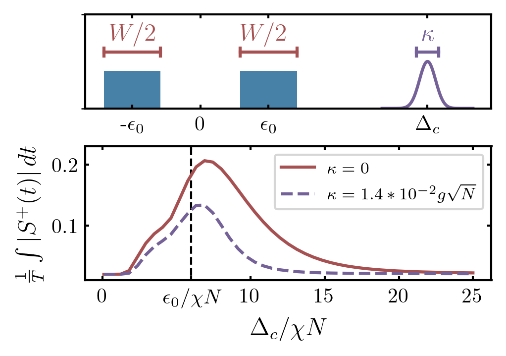
Figure 1: Top panel: A simple schematic of the distribution of atomic levels (see text) and the spectral response of the cavity with detuning $\Delta_{c}$ and linewidth $\kappa$. Bottom panel: Time average of the phase coherence $S^{+}=\frac{1}{N}\sum_{i}\left<\hat{\sigma}^{+}_{i}\right>$ as a function of the cavity detuning $\Delta_{c}/(\chi N)$, for large disorder $W/(\chi N)=8$. In the adiabatic limit, $\Delta_{c}/(\chi N)\rightarrow\infty$, the simulator shows vanishing coherence, $S^{+}(t)\rightarrow 0$, while coherence is maximum when the photon is at resonance with the mean atomic transverse field $\Delta_{c}\approx\epsilon_{0}=6\chi N$ (marked by a black dashed line). To make use of an integrability analysis we assume an ideal cavity with $\kappa=0$ for most of the paper, and then confirm that a realistic cavity linewidth, $\kappa/(g\sqrt{N})=1.4\times 10^{-2}$, does not significantly modify the resonance phenomenon.

Such an emulator has been proposed in AMO physics for quantum simulation of archetypal s-wave superconductors (for charged particles) or s-wave superfluids (for neutral particles) Smale et al. (2019); Lewis-Swan et al. (2021) . In these works the dynamics of the superfluid phase coherence, directly related to the Meisner and Anderson-Higgs mechanisms in superconductors Annett (2004), can be studied by monitoring the dynamics of the atomic phase coherence. In the QED simulators considered so far, the cavity must be far detuned from atomic frequencies so that photonic degrees of freedom can be integrated out Agarwal et al. (1997); Damanet et al. (2019); Kelly et al. (2021); Muniz et al. (2020); Norcia et al. (2018); Palacino and Keeling (2020); Davis et al. (2019); Periwal et al. (2021); Vaidya et al. (2018); Marsh et al. (2021); Seetharam et al. (2021); Klinder et al. (2015); Mivehvar et al. (2021); Baumann et al. (2010); Brennecke et al. (2007); Fogarty et al. (2015); Habibian et al. (2013); Himbert et al. (2019); Keller et al. (2018, 2017); Schütz et al. (2016); Xu et al. (2016) and so an effective matter-only s-wave model of superconductivity is sufficient to describe the dynamics. In such a limit the cavity only contains virtual photons, and their primary purpose is to mediate pairing interactions.

In this Letter, we investigate the effect of real photons on the phase coherence when the cavity detuning to the atomic transition is reduced. In this limit, the single channel s-wave BCS Hamiltonian is no longer an accurate description, and instead the atoms and cavity field simulates the two channel model of the BCS-BEC crossover Yuzbashyan et al. (2015); Annett (2004). In this model, the effect of reducing photon detuning on the dynamics are non-trivial because, on one hand, reducing the detuning yields a stronger mediated interaction strength, while on the other hand reducing the detuning leads to retarded photon dynamics where an instantaneous interaction is no longer valid. Here, we find that even when the change in interaction strength is accounted for, the retarded photon dynamics can maintain phase coherence better than the instantaneous interaction. This is demonstrated in Fig. 1, where we show that upon reducing the photon detuning phase coherence increases until resonance, below which the diabatic (small detuning) limit takes over and phase coherence is lost. While these results are mostly obtained by a classical integrability analysis Dukelsky et al. (2004a); Richardson (2002); Barankov and Levitov (2006); Barankov et al. (2004); Yuzbashyan et al. (2005a, b, 2006, 2015), we also find via numerical simulation that the phenomenon is robust to the non-integrable effects caused by inhomogeneous couplings and photon loss which are typically present in realistic cavity QED settings.

Simulation of Superfluid Phase Coherence. We consider the simulation of the two-channel model for the BCS-BEC crossover observed in ultracold fermion experiments Yuzbashyan et al. (2015); Annett (2004). The model involves fermions (with creation operator $\hat{f}^{\dagger}_{\textbf{k},s}$ with momentum vector k and spin $s$) that can form Cooper pairs on the BCS side of the crossover or, bind into diatomic bosonic molecules at zero center of mass momentum (with creation operator $\hat{d}^{\dagger}$) on the BEC side of the crossover. Neglecting finite momentum molecular bosons, the dynamics are characterized by the Hamiltonian:

$$H_{f}/\hbar = \sum_{\textbf{k},s}\epsilon_{\left|\textbf{k}\right|}\hat{f}^{\dagger}_{\textbf{k},s}\hat{f}_{\textbf{k},s}+g\sum_{\textbf{k}}\hat{f}^{\dagger}_{\textbf{k},\uparrow}\hat{f}^{\dagger}_{-\textbf{k},\downarrow}\hat{d}+h.c.+\Delta_{c}\hat{d}^{\dagger}\hat{d},$$

where $\hat{d}$ is the mean molecular field, $\Delta_{c}$ is the molecular binding energy, and $g$ is the coupling strength between fermions and molecules. When the fermions condense into a superfluid on the BCS side of the crossover, they mostly form Cooper pairs Annett (2004) quantified by the complex pair amplitudes $\rho_{\textbf{k}}=\langle\hat{f}^{\dagger}_{\textbf{k},\uparrow}\hat{f}^{\dagger}_{-\textbf{k},\downarrow}\rangle$. In this Letter, we focus on the dynamics of the superfluid s-wave phase coherence $S^{+}=\frac{1}{N}\sum_{\textbf{k}}\rho_{\textbf{k}}$, which quantifies the phase coherence between Cooper pairs with different pairing wave vector k.

Similar to Ref. Lewis-Swan et al. (2021), the Cooper pairs can be simulated by a collection of two level atoms (described by Pauli operators $\hat{\sigma}^{+}_{i}$ and $\hat{\sigma}^{z}_{i}$) via the Anderson pseudospin mapping Barankov and Levitov (2006); Barankov et al. (2004); Yuzbashyan et al. (2015):

$$\leavevmode\resizebox{375.80542pt}{}{ $\hat{\sigma}^{+}_{i}\rightarrow\hat{f}^{\dagger}_{\textbf{k}_{i},\uparrow}\hat{f}^{\dagger}_{-\textbf{k}_{i},\downarrow},\quad\hat{\sigma}^{z}_{i}\rightarrow\hat{f}^{\dagger}_{\textbf{k}_{i},\uparrow}\hat{f}_{\textbf{k}_{i},\uparrow}+\hat{f}^{\dagger}_{-\textbf{k}_{i},\downarrow}\hat{f}_{-\textbf{k}_{i},\downarrow}-1$}.$$ (1)

where each atom $i$ simulates a pair of fermion momentum modes $i\rightarrow\pm\textbf{k}_{i}$. The above Hamiltonian can then be simulated by a cavity QED system similar to the experiments described in references Norcia et al. (2018); Norcia and Thompson (2016); Muniz et al. (2020); Davis et al. (2019), in which the internal levels of $2N$ atoms are encoded in long lived electronic states, e.g the ${}^{1}S_{0}$-${}^{3}P_{1}$ states of ⁸⁸Sr atoms. The atoms are trapped in an optical lattice and are allowed to interact with a single cavity mode (described by a photon annihilation operator $\hat{a}$ simulating the molecular field, $\hat{a}\rightarrow\hat{d}$). Such a system is modeled by the Hamiltonian Norcia et al. (2018); Muniz et al. (2020); Lewis-Swan et al. (2021):

$$H/\hbar=\sum_{i=1}^{2N}\epsilon_{i}\hat{\sigma}^{z}_{i}+\sum_{i=1}^{2N}g_{i}(\hat{\sigma}^{\dagger}_{i}\hat{a}+h.c.)+\Delta_{c}\hat{a}^{\dagger}\hat{a},$$ (2)

where $\Delta_{c}$ is the detuning of the cavity from the mean atomic frequency, $2g_{i}$ is the single-photon Rabi frequency, and $\epsilon_{i}$ is an inhomogeneous effective transverse field. Simulation of $H_{f}$ by the cavity QED system occurs for homogenous light-matter coupling $g_{i}=g$ and for a probability distribution, $p(\epsilon_{i})$, of the inhomogeneous field, $\epsilon_{i}$, that is designed to match the density of states for the fermion model. We choose the density of states as $p(\epsilon_{i})=\left[B(W/2,\epsilon_{0}/2,\epsilon_{i})+B(W/2,-\epsilon_{0}/2,\epsilon_{i})\right]/2$, where $B(\alpha,x_{0},x)$ is a box distribution with mean $x_{0}$ and width $\alpha$ (see Fig. 1). Similar to Ref. Lewis-Swan et al. (2021), such a bimodal distribution is chosen to ensure the possibility of persistent oscillations of the phase coherence (see below) in the $W=0$ limit. A possible band structure reproducing this density of states and the superfluidity that would occur in the traditional thermal equilibrium setting is discussed in Ref. .

At large detuning, $\Delta_{c}\gg g\sqrt{N}$ and $\Delta_{c}\gg\epsilon_{0}+W/2$, the cavity field mediates spin-exchange interactions and an effective spin model can be derived which maps into a one channel BCS model as discussed in Ref. Lewis-Swan et al. (2021). In this limit, an adiabatic approximation Norcia et al. (2018); Muniz et al. (2020); Lewis-Swan et al. (2021) assumes the state of the light field is in instantaneous equilibrium such that $\left<\hat{a}_{eq}^{\dagger}(t)\right>=-\frac{gN}{\Delta_{c}}S^{+}$, where $S^{+}=\frac{1}{N}\sum_{i}\left<\sigma_{i}^{+}\right>=\frac{1}{N}\sum_{\textbf{k}}\rho_{\textbf{k}}$ is both the atomic phase coherence and the simulated superfluid phase coherence. Thus, in the large detuning limit, the photon directly measures the phase coherence $S^{+}$. Inserting $\left<\hat{a}_{eq}^{\dagger}(t)\right>$ back into Eq. 2 and taking homogenous couplings, one finds a mediated interaction $-\chi\sum_{ii^{\prime}}\hat{\sigma}^{+}_{i}\hat{\sigma}^{-}_{i^{\prime}}$ with interaction strength $\chi=g^{2}/\Delta_{c}$ and sign which favors effective Cooper pair formation at low temperatures and positive detuning, $\Delta_{c}$. In this work we will study the dynamics when the photon detuning, $\Delta_{c}$, is decreased and the adiabatic approximation is no longer valid. One complication to this limit is that when the photon detuning is decreased, the interaction strength $\chi$ increases. To isolate this effect we imagine that the experiment simultaneously increases the strength of the atomic energies as the photon detuning is decreased such that $\epsilon_{0}/\chi N$ and $W/\chi N$ are held constant.

Dynamical Phases from classical integrability. To study the dynamics of this system, we make a mean field approximation (i.e. $\langle\hat{O}_{1}(t)\hat{O}_{2}(t)\rangle=\langle\hat{O}_{1}(t)\rangle\langle\hat{O}_{2}(t)\rangle$ and adopt the notation: $\langle\hat{O}_{1}\rangle\equiv O_{1}$) which is expected to work up to time scales $O(1/(\chi N))$ Kirton and Keeling (2017, 2018); Kirton et al. (2019). The resulting classical dynamics of the Hamiltonian in Eq. 2 show Richardson Gaudin integrability Dukelsky et al. (2004a); Richardson (2002); Barankov and Levitov (2006); Barankov et al. (2004); Yuzbashyan et al. (2005a, b, 2006, 2015); Dukelsky et al. (2004b); Richardson and Sherman (1964); Gaudin (1976) in the homogenous limit, $g_{k}=g$ . The so called Lax integrability analysis Dukelsky et al. (2004a); Richardson (2002); Barankov and Levitov (2006); Barankov et al. (2004); Yuzbashyan et al. (2005a, b, 2006, 2015) is then used to study the integrable tori of the classical mean field Hamiltonian corresponding to Eq. 2 and to construct a dynamical phase diagram Lewis-Swan et al. (2021); Yuzbashyan et al. (2015) characterizing the collective modes. This is done by studying the conserved quantities to identify a minimum number, $M$, of collective degrees of freedom (DOF) required to effectively reproduce the dynamics of collective variables at long times .

The dynamical phases are then classified by the required number of collective DOF and the dynamics of the phase coherence $S^{+}$. First, we consider the resulting collective modes for a quench starting from an initial state with all spins polarized in the $\hat{x}$ direction, $\left<\hat{\sigma}^{x}_{i}\right>=1$, and the cavity in the vacuum, $\left<a\right>=0$. In the spin-only model, three phases are found Yuzbashyan et al. (2015); Lewis-Swan et al. (2021) with at most $M=2$. In contrast, we identify a fourth phase with $M=3$ upon introducing the photon away from adiabatic elimination. The three phases in the adiabatic limit, $\Delta_{c}\rightarrow\infty$, are (for fixed $\chi N$ and $\epsilon_{0}>\chi N$):

• Phase I ($M=0$): At large disorder, all phase coherence is lost, and the simulated superfluid enters a normal state: $S^{+}(t)\rightarrow 0$.

• Phase II ($M=1$): Transition to this phase occurs as disorder is reduced, and involves only one effective degree of freedom ($M=1$). In this phase, the magnitude of the phase coherence, $\left|S^{+}(t)\right|$, is constant at late time, and the collective mode corresponds to precession of the phase of $S^{+}$: $S^{+}(t)\rightarrow\left|S^{+}\right|e^{i\mu t}$.

• Phase III ($M=2$): This phase occurs at even smaller inhomogeneous atomic broadening, and has $M=2$ DOF. The collective mode shows persistent oscillations in $\left|S^{+}(t)\right|$ as shown in the lower panel of Fig. 2.

In this adiabatic limit, the critical disorder strengths between phase I and II, and II and III, depends non-trivially on $\epsilon_{0}$, but are on the order of the interaction strength $\chi N$.

At finite detuning, $\Delta_{c}$, the photon becomes another DOF in the collective oscillations of these three phases, and to distinguish the phases of the full model we will write them with a “$+1$” superscript. The phases $I^{+1}$ and $II^{+1}$ show the same qualitative dynamics of $S^{+}(t)$ as the phases $II$ and $III$ respectively, while a new phase $III^{+1}$ is defined by aperiodic oscillations of $\left|S^{+}(t)\right|$ and requires $M=3$ collective DOF (two macroscopically coherent spins and a photon). At large but finite $\Delta_{c}$, the new phase $III^{+1}$ involves the photon performing fast oscillations around $a_{eq}(t)$, the slowly evolving equilibrium value given by adiabatic elimination (see Fig. 2 for an example). In this limit, the aperiodic contribution to the oscillations of $S^{+}$ becomes small smoothly as function of $\Delta_{c}$, and thus in the large detuning limit phase $III^{+1}$ approximates phase $III$. This limiting behavior is the same for phases $I^{+1}$ and $II^{+1}$ which, for large detuning, approximate phase $I$ and $II$ respectively.

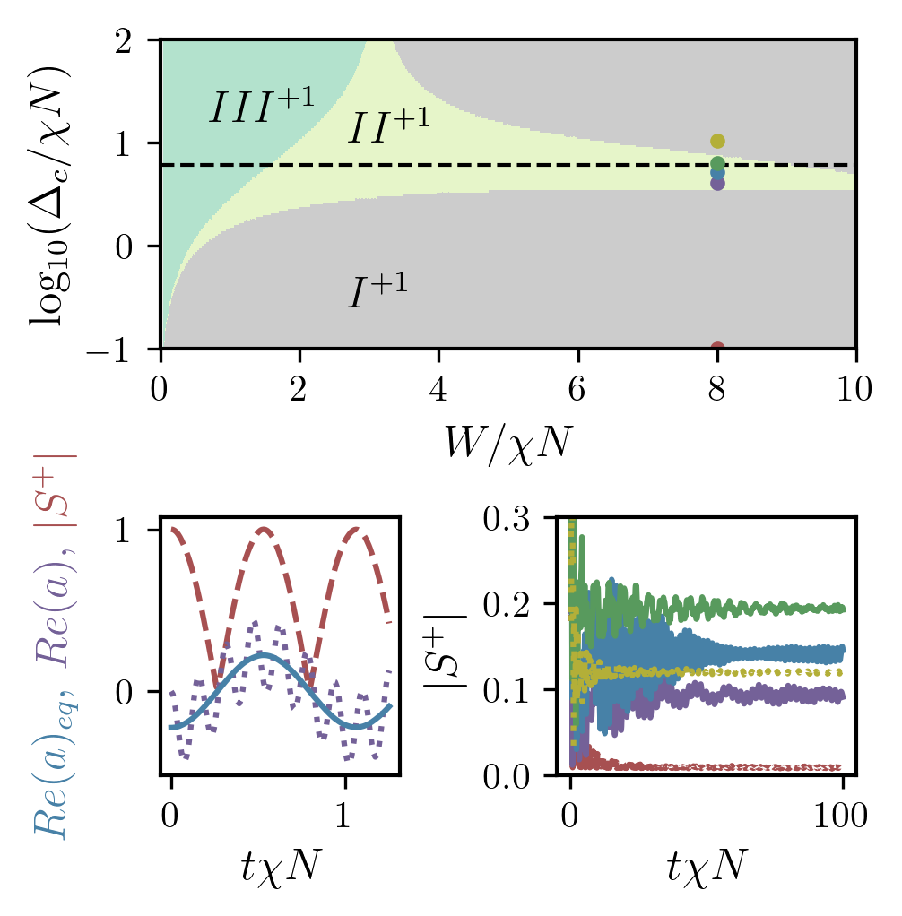
Figure 2: The top panel shows the dynamical phase diagram as a function of the cavity detuning and atomic disorder. The approximate resonance condition, $\Delta_{c}\approx\epsilon_{0}=6\chi N$, is marked by a black dashed line. The bottom left panel shows dynamics characteristic of phase $III^{+1}$ (specifically $W=0$ and $\Delta/(\chi N)=40$). For these parameters, the adiabatic approximation correctly predicts the dynamics of the matter, but misses the extra oscillation around $a_{eq}(t)$ predicted by the Lax analysis. The bottom right panel shows the dynamics of $\left|S^{+}(t)\right|$ for $W/(\chi N)=8$ and different values of $\Delta_{c}/(\chi N)$ marked in the top panel. For $\Delta_{c}/(\chi N)=0.1$ (red) and $10.3$ (yellow), $\left|S^{+}(t)\right|$ evolves to a constant steady state characteristic of phase $I^{+1}$, while for the remaining values of $\Delta_{c}/(\chi N)$ the dynamics have persistent oscillations characteristic of phase $II^{+1}$. In this figure, the initial state has $\left<\hat{\sigma}^{x}_{i}\right>=1$ and $\left<a\right>=0$.

Upon reducing the detuning, a rich dynamical phase diagram emerges as shown in the upper panel of Fig 2. In the $W=0$ limit, there is only phase $III^{+1}$, while, at finite $W$, the cavity field has a broad impact on the dynamical phase diagram. In the diabatic limit, $\Delta_{c}/\chi N\ll 1$, the dynamics are much more sensitive to the inhomogeneities due to an inability of the cavity to mediate an effective interaction, and the transition to phase $I^{+1}$ occurs at much smaller disorder in comparison to the large detuning limit. We also find a region at large disorder, $W>4\chi N$, where phase $II^{+1}$ occurs when $\Delta_{c}\sim\epsilon_{0}$ which suggests phase coherence can be enhanced by setting the detuning on resonance with the atoms that have atomic energies close to $\epsilon_{0}$.

Mechanism of resonant phase coherence. The enhancement of phase coherence is confirmed in Fig. 1, and we explain the formation of this resonance by first considering finite but large detuning, such that $1/\Delta_{c}$ is still the fastest timescale. In this limit the dynamics are in Phase $I^{+1}$ and the enhancement of phase coherence is very weak at long times, but the following simple picture holds. First, on a timescale of $1/\Delta_{c}$, the initial polarization of the spins drive the photon into an excited state oscillating around a non-zero $a_{eq}(t=0)=-Ng/\Delta_{c}$. Then, on a timescale of $1/W\gtrsim 1/\Delta_{c}$, the spins mostly dephase and $a_{eq}(t\rightarrow\infty)\approx 0$. Once the spins mostly depolarize to their steady state, the photon remains oscillating around a small equilibrium, $a(t)\approx Ae^{i\mu t}$. The Lax analysis (see Yuzbashyan et al. (2015) and Note (1)) yields expressions for the frequency and amplitude of these small oscillations which have a simple analytical form when $\Delta_{c}>W>\epsilon_{0}$: $\mu=\Delta_{c}$ and $A=\chi N/g=\sqrt{N}\sqrt{\chi N/\Delta_{c}}$.

From the perspective of the matter, the photon is effectively an external drive that pumps a small fraction of the spins into a coherent steady state. In the frame of reference of the photon (the effective external drive), the dynamics of each spin is fully described by a constant magnetic field, $\vec{h}=(\epsilon_{i}-\mu)\hat{z}+gA\hat{x}$, and we can solve for the steady state as:

$$S^{+}=\frac{1}{N}\sum_{i}\frac{gA}{\sqrt{(\epsilon_{i}-\mu)^{2}+\left|gA\right|^{2}}}.$$ (3)

Since $\mu\sim\Delta_{c}$, this expression correctly predicts the loss of coherence, $S^{+}$, in the adiabatic limit shown in Fig. 1.

Further away from the adiabatic limit, the separation of time scales, $1/W\gtrsim 1/\Delta_{c}$, that yields the simple picture above is no longer valid. Regardless, the Lax analysis still produces the same expression, Eq. 3, for the phase coherence in phase $I^{+1}$ but now with a different $A$ and $\mu$ that must be numerically determined by solving for the roots of a Lax vector (see Yuzbashyan et al. (2015) and SM). Since $\mu$ gives the precession frequency of the photon, it is expected to be close to the detuning $\mu\approx\Delta_{c}$ and this is what we find numerically. Eq. 3 therefore predicts the atom at site $i$ will be in resonance when $\Delta_{c}=\epsilon_{i}$. The coherence is then maximally enhanced when most spins are driven close to resonance and occurs when the drive, $\Delta_{c}$, is at the center of the band of atomic frequencies $\Delta_{c}\approx\epsilon_{0}$. This approximation is confirmed by the peak in coherence shown in Fig 1.

Although Eq. 3 provides an intuitive picture, simliar to a single particle resonance, when the system is in phase $I^{+1}$, the relevant enhancement of coherence at the resonance happens in phase $II^{+1}$ where the cavity field and atomic coherence must both be treated as dynamical variables. As shown in Fig. 2, their dynamics in this regime show coupled nonlinear oscillations Yuzbashyan et al. (2015).

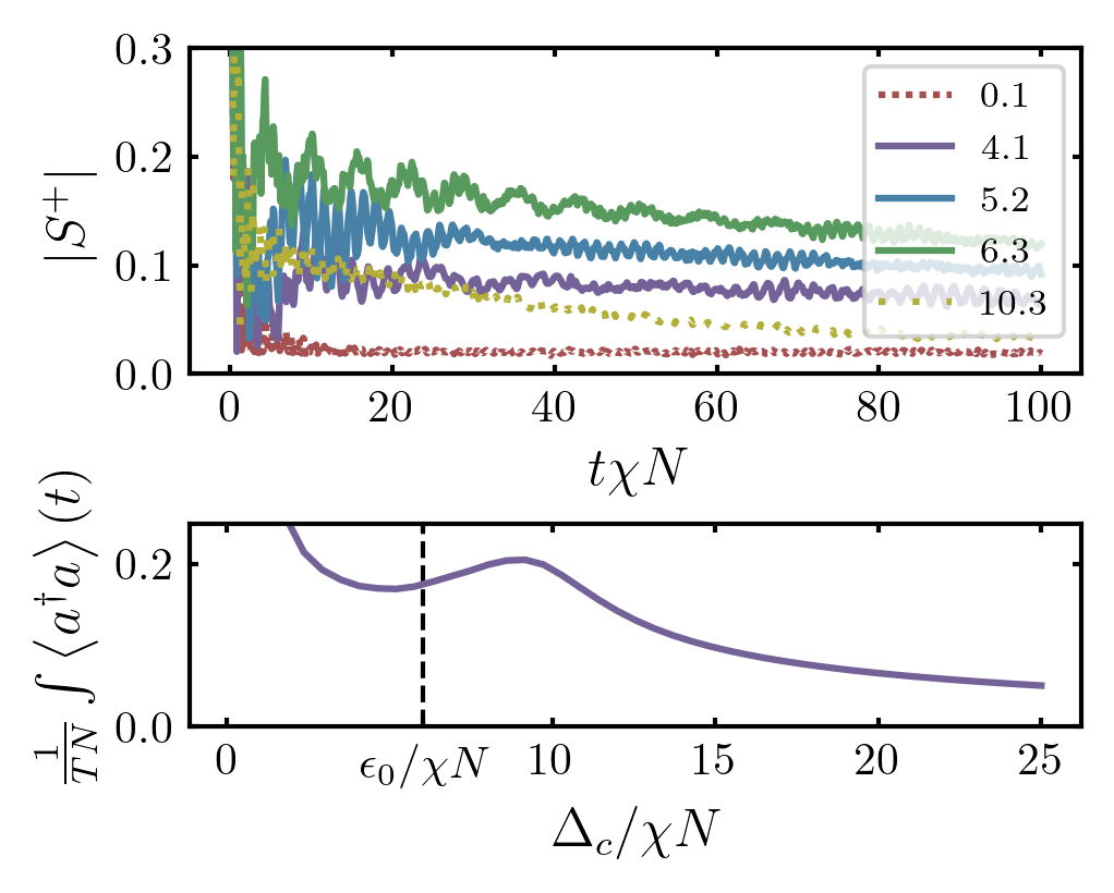
Figure 3: The top panel shows the same dynamics for $\left|S^{+}(t)\right|$ as in Fig. 2, but with $\kappa/(2\pi)=150~{}{\rm kHz}$ and $g/(2\pi)=10.8~{}{\rm kHz}$ as in the experiments of Muniz et al. (2020); Norcia et al. (2018). The bottom panel is computed assuming inhomogeneous couplings and an initial state prepared by a coherent drive through the cavity. Even though inhomogeneities and cavity losses reduce the coherence, we can observe a signature of the resonance as a minimum Note (4) in the photon density. Note that in contrast to Fig. 2 and Fig. 1, the initial state depends on the initial number of photons driven into the cavity which scales as $1/\Delta_{c}$. Both figures were obtained by numerical simulation of the Lindblad equations of motion at mean-field Note (3). In the top panel, the decay rate of $\left|S^{+}(t)\right|$ is constant with $\Delta_{c}/\chi N$ and proportional to $1/\kappa$, but appears to increase with $\Delta_{c}/\chi N$ in the figure because the unit for time, $1/\chi N$, decreases with $\Delta_{c}$ when $g$ is fixed.

Experimental Realization. In the experiments of Refs. Muniz et al. (2020); Norcia et al. (2018) an optical lattice is used to trap Sr atoms, featuring a long-lived electronic clock transition with atomic decay rate of $\gamma$. The optical lattice is placed inside a standing wave optical cavity with linewidth $\kappa$. While both $\gamma$ and $\kappa$ destroy phase coherence at long times, we find that the effect of resonant phase coherence is still observable on times $O(1/\kappa)$ provided we operate at large collective cooperativity ($Ng^{2}\gg\kappa\gamma$). Given that for long-lived Sr atoms, $\kappa\gg\gamma$ we neglect atomic decay. Fig. 1 shows the dependence of $\left|S^{+}(t)\right|$ on $\Delta_{c}$, and demonstrates that the resonant enhancement can be maintained even with cavity loss. Furthermore, Fig. 3 depicts how the dynamics in Fig. 2 simply features a slow decay for moderate $\kappa$.

The experiments in Muniz et al. (2020); Norcia et al. (2018) also have inhomogeneous couplings $g_{i}=g\cos(k_{0}a_{0}i)$ with $k_{0}a_{0}=3.7$ due to an incommensurability between the optical lattice spacing, $a_{0}$, and the cavity wavelength, $2\pi/k_{0}$. The inhomogeneous couplings will disrupt the effect discussed in this work if we start in a homogenous state, since the couplings will no longer excite the photon. However, as long as the initial state is generated by coherently driving the optical cavity, inhomogeneities do not play a detrimental effect. In this case, the initial state involves all spins aligned with the inhomogeneities $\text{sgn}(\sigma^{x}_{i})=\text{sgn}(g_{i})$ such that cavity will be coherently pumped by the atoms. The resulting simulations show signature of resonant phase coherence as a minimum  of the time averaged photon density shown in Fig. 3. Note that both dissipation and inhomogeneities break Lax integrability.

Conclusion. Our work demonstrates that dynamical fluctuations of a mediating field can produce enhancement of phase coherence in cavity QED simulators of superconductivity and superfluidity. The generality of our result based on a resonance argument, would suggest a natural extension to a broad variety of platforms such as trapped ions or quantum optics in waveguides, both of which serve as tunable simulators of non-equilibrium quantum many body physics, employing mediating photons or phonons Bruzewicz et al. (2019); Chang et al. (2018). It also suggests a promising direction for cavity enhanced superconductivity in real materials. Such a possibility requires extending the phenomenon to charged superfluids in which the light-matter couplings are structurally different from the atom-molecule couplings of Eq. 1. Our results offer the possibility of studying novel regimes of enhanced cooperative light-matter, and hint that quantum many-body optics with active light and matter degrees of freedom has the potential to become a blossoming area of quantum simulation in the near future.

Acknowledgments– This work has been funded by the Deutsche Forschungsgemeinschaft (DFG, German Research Foundation) - TRR 288 - 422213477 (project B09), TRR 306 QuCoLiMa (”Quantum Cooperativity of Light and Matter”), Project-ID 429529648 (project D04) and in part by the National Science Foundation under Grant No. NSF PHY-1748958 (KITP program ‘Non-Equilibrium Universality: From Classical to Quantum and Back’). A. M. R. acknowledges ARO (Army Research Office) under the Grant No. W911NF-19-1-0210, and the National Science Foundation under the Grants No. NSF PHY1820885. Both A.M.R and J.K.T acknowledge NSF JILA-PFC PHY-1734006, QLCI-OMA -2016244, the U.S. Department of Energy, Office of Science, National Quantum Information Science Research Centers Quantum Systems Accelerator, and NIST.

Appendix A Lax analysis for quench dynamics

In the main text, we studied the dynamics of an initial state with $\left<\sigma^{x}_{i}\right>=1$ and with the photon in an empty cavity state. Here, we consider a more general state used in Lewis-Swan et al. (2021) where the spins $1\dots N$ point in the $\hat{x}\cos(\Delta\phi_{0}/2)+\hat{y}\sin(\Delta\phi_{0}/2)$ direction, while the spins $N+1\dots 2N$ point in the $\hat{x}\cos(\Delta\phi_{0}/2)-\hat{y}\sin(\Delta\phi_{0}/2)$ direction, and the photon is either in the vacuum, $a(t=0)=0$ or at equilibrium with matter, $a(t=0)=a_{eq}(0)=-\frac{1}{\Delta_{c}}\sum_{i}g_{i}\sigma^{-}_{i}(t=0)$.

We now compute the lax vector for such a state:

$$\vec{L}(u,t)=\sum_{i}\frac{\vec{\sigma}_{i}(t)}{u-\epsilon_{i}}+\hat{z}\frac{2}{g^{2}}(u-\Delta_{c}/2)-\frac{2\vec{\Delta}(t)}{g^{2}}$$ (4)

Since the initial state is uniform for spins $1\dots N$ and for $N+1\dots 2N$, the sums over $i$ splits into two sums which can be approximated by disorder average:

$$\sum_{i}\frac{1}{u-\epsilon_{i}}\approx N\int\frac{p(\epsilon)}{u-\epsilon}d\epsilon$$ (5)

where $p(\epsilon)$ is the disorder distribution for transverse fields: $\epsilon_{i}=\epsilon/2+x_{i}$ for $i\in(1\dots N)$ and $\epsilon_{i}=-\epsilon/2+x$ for $i\in(N+1\dots 2N)$, and $x_{i}$ are drawn from a uniform distribution with zero mean and width $W/2$. The integral results in a logarithm whose branch cut must be chosen to match the continuum of poles that develop when taking the $N\rightarrow\infty$ limit of the summationYuzbashyan et al. (2005a, b, 2006). This results in:

$$\lim_{N\rightarrow\infty}\frac{\chi}{2}\sum_{i}\frac{\sigma^{y}_{i}(t=0)}{u-\epsilon_{i}} =L^{y}_{l}(u)= \frac{\chi N}{W}\sin(\frac{\Delta\phi_{0}}{2})\ln\left[\frac{(4u)^{2}-(W-2\epsilon_{0})^{2}}{(4u)^{2}-(W+2\epsilon_{0})^{2}}\right]$$ (6)

$$\lim_{N\rightarrow\infty}\frac{\chi}{2}\sum_{i}\frac{\sigma^{x}_{i}(t=0)}{u-\epsilon_{i}} =L^{x}_{l}(u)= 2\frac{\chi N}{W}\cos(\Delta\phi/2)\left[\text{Arctanh}(\frac{W-2\epsilon_{0}}{4u})+\text{Arctanh}(\frac{W+2\epsilon_{0}}{4u})\right],$$

where the branch cut for $\text{ln}(x)$ is $Re(x)\in[0,-\infty)$, and the branch cut for $\text{ArchTanh}(x)$ is $Re(x)\in[-1,-\infty)$ and $Re(x)\in[1,\infty)$. The square lax vector is therefore computed as:

$$\frac{\chi}{2}\vec{L}^{2}=\left(\chi\vec{L}^{x}_{l\perp}(u)-s\frac{\chi N}{\Delta_{c}}\cos(\Delta\phi/2)\right)^{2}+\chi\vec{L}^{y}_{l\perp}(u)^{2}+\left(1-\frac{2u}{\Delta_{c}}\right)^{2}$$ (7)

where $s=0$ if the cavity field is $a(t)=0$ at $t=0$, or $s=1$ if the cavity field is in equilibrium with matter $a(t=0)=a_{eq}(t=0)$ at $t=0$.

In the main text, we used the numerical search described below to study the dynamical phases as a function of $\Delta_{c}/\chi N$ and $W/\chi N$, for fixed $\epsilon_{0}/\chi N=6$, $\Delta\phi_{0}=0$ and photon starting in the vacuum. Such a phase diagram does not qualitatively change by increasing $\Delta\phi$, but if the cavity field is in equilibrium with matter $a(t=0)=a_{eq}(t=0)$ at $t=0$, and $\Delta\phi_{0}=\pi$ we see larger region for phase $II^{+1}$ (see Fig 4).

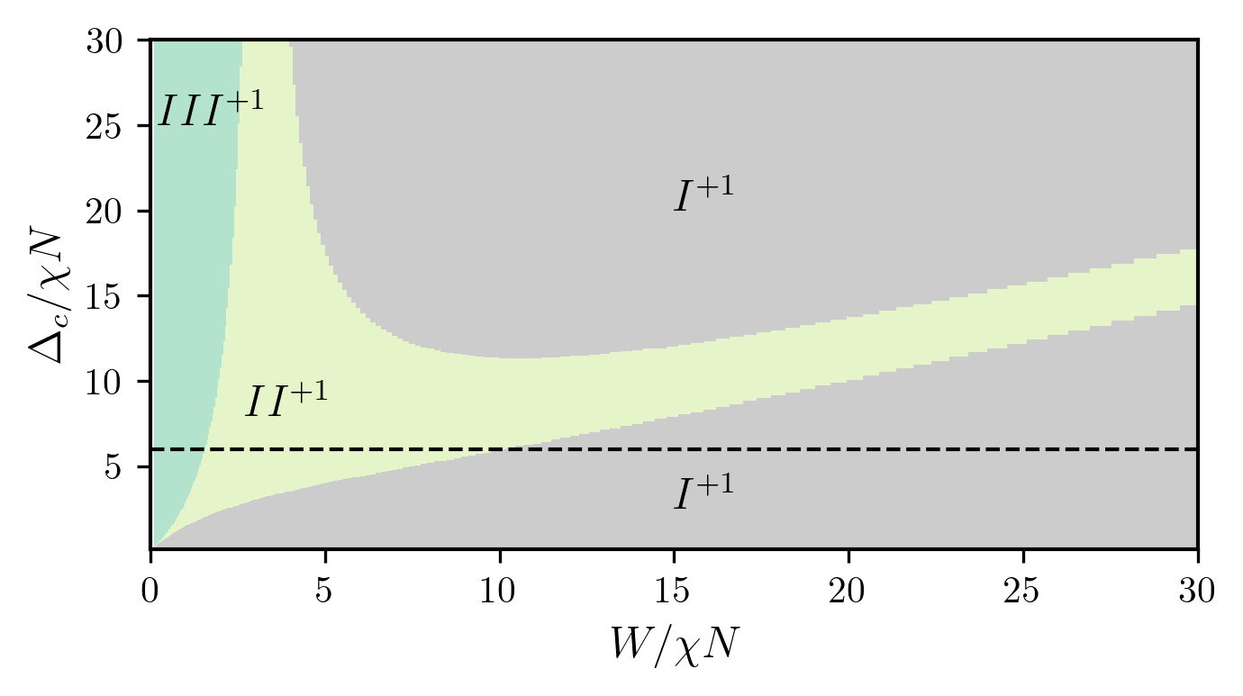
Figure 4: Phase diagram as in main text but for an initial state with $\Delta\phi_{0}=\pi$ and $a(0)=a_{eq}(0)$. Interestingly, for large $W$, the region of Phase $II^{+1}$ shifts to higher frequencies. While this region is in phase $II^{+1}$ where the amplitude $\left|S^{+}\right|$ oscillates, the oscillations and over all phase coherence are relatively small at large $W$. Similarly, the Lax analysis of phase $I^{+1}$ still predicts a resonance in phase coherence $\left|S^{+}\right|$ at $\Delta_{c}=\epsilon_{0}$ (marked by a black dashed line); we have confirmed this numerically.

A.1 Numerical Search for the roots

The dynamical phases are characterized by the number of roots of $\vec{L}^{2}(u)=0$ as discussed in the main text. To find these roots for a range of $W/\chi N$ and $\Delta_{c}/\chi N$ as in the main text, we employ the NLsolve Julia library. The algorithm requires an initial seed for the roots and then uses the steepest decent to find the numerical value. Therefore, to find all the unique roots $\vec{L}^{2}(u)=0$ and thereby correctly identify the dynamical phase we perform the following process. First, we plot the complex magnitude of $\vec{L}^{2}(u)$ and identify an approximate location of the 6 roots from the plot. Then we use NLsolve function to find a precise location of the root with a relative and absolute numerical error tolerance of $10^{-4}$. For the first root, this is done for $W=0$, a specific initial state, a large value of $\Delta_{c}/\chi N$, and the remaining Hamiltonian parameters fixed.

Since the location of the roots are smoothly connected to each other as $\Delta_{c}/\chi N$ is smoothly decreased, we next find the location of roots for $W/\chi N=0$ and different values of $\Delta_{c}/\chi N$. This is done by starting with roots found for $W=0$ and the large value of $\Delta_{c}/\chi N$ and then finding the roots sequentially decreasing $\Delta_{c}/\chi N$. The seeds used for the NLsolve function are the roots obtained from the previous step in the sequence with slightly larger $\Delta_{c}/\chi N$. Then, starting with the root found for a specific $\Delta_{c}/\chi N$ and $W/\chi N=0$, we find the roots for $W/\chi N>0$ performing a similar sequential process, but this time increasing $W/\chi N$ and keeping $\Delta_{c}/\chi N$ fixed. After finding all the roots, we identify the unique ones, up to an error tolerance of $10^{-4}$, to identify which phase we are in.

A problem that can arise in this process is two roots closely approach each other, as $W/\chi N$ is increased. If this occurs, the seeds used for steepest decent can become identical to each other in the sequential update of seeds based on the previous roots. In order to prevent such issue, we keep a list of fixed seeds that we also use when finding distinct roots at each point in the phase diagram.

A.2 Analytic solution for phase $I^{+1}$ roots

As discussed in the main text, the location of the two roots in phase $I^{+1}$ gives useful information on the dynamics of the photon. These roots can be found if

$$\Delta_{c}>W>\epsilon_{0},$$ (8)

when the cavity is initially empty, and when $\Delta\phi_{0}=0$. In this limit, the ArchTanh can be expanded, and the Lax squared vector yields:

$$\chi/2\vec{L}^{2}\approx(\frac{4\chi N}{W})^{2}(\frac{W}{4u})^{2}+(1-\frac{2u}{\Delta_{c}})^{2}+...$$ (9)

Defining $u=u^{\prime}\Delta_{c}/2$, the condition $\vec{L}^{2}(u)=0$ becomes:

$$\pm i\frac{2\chi N}{\Delta_{c}}\frac{1}{u^{\prime}}=1-u^{\prime}$$

The quadratic equation solves as

$$u^{\prime}=\frac{1\pm\sqrt{1\pm i8/\Delta_{c}^{\prime}}}{2}.$$ (10)

When $\Delta_{c}^{\prime}=\Delta_{c}/\chi/N$ is very large the small angle approximation yields $u^{\prime}\approx 1\pm i\frac{2}{\Delta_{c}^{\prime}}$, or $u=\frac{\Delta_{c}}{2}\pm i\chi N$. The Lax analysis argues Yuzbashyan et al. (2015) that in Phase $I^{+1}$, the real and imaginary parts of this root pair gives the frequency, $\mu$, and amplitude, $A$, of the photon oscillations respectively: $a\approx Ae^{i\mu t}$. Therefore we find that when, $\Delta_{c}>W>\epsilon_{0}$ the photon frequency is given as $\mu=\Delta_{c}$ the photon amplitude as $A=\chi N/g=\sqrt{N}\sqrt{\chi N/\Delta_{c}}$. as in the main text. This is confirmed in Fig. 5.

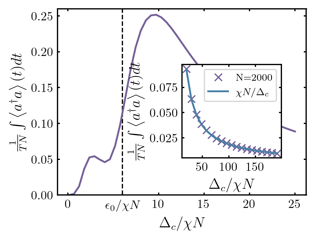
Figure 5: This figure shows the effect of resonant phase coherence as monitored by the photons. Since in the adiabatic limit $a^{\dagger}\rightarrow-gNS^{+}/\Delta_{c}$, and $S^{+}$ vanishes at long times for the chosen conditions, it directly quantifies the extent to which adiabatic elimination fails. The inset shows numerical confirmation (marked by x’s) of the analytic prediction for the photon amplitude $A^{2}=N^{2}\chi/\Delta_{c}$ (solid line). Such a prediction requires the approximation $\epsilon_{0}\ll W$, and therefore $\epsilon_{0}=\chi N\ll W=8\chi N$ in the inset, while in the main figure $\epsilon_{0}=6\chi N$. In both, the initial state has $\left<\hat{\sigma}^{x}_{i}\right>=1$ and $\left<a\right>=0$.

Appendix B Minimum in photon occupation at resonance

As seen in Fig. 5, and in Fig. 3 of the main text, the photon density $\frac{1}{TN}\int_{0}^{T}dt\left<a^{\dagger}a\right>$ shows a minimum as a function of the detuning, $\Delta_{c}$, near resonance $\Delta_{c}=\epsilon_{0}$. This phenomenon is explained in a similar way to the resonance maximum seen by the phase coherence $\left|S^{+}\right|$ and it is related to the conservation of total excitations: $S^{z}+a^{\dagger}a$. In Fig. 5, the initial state is polarized in the $\hat{x}$ direction and with no photons in the cavity such that $S^{z}+a^{\dagger}a=0$. Therefore the photon density is fixed to the $J_{z}$ polarization of the spins: $a^{\dagger}a=-S^{z}$. Using the same argument in the main text that, in phase $I^{+1}$, the photon simply acts as an external drive with $a=Ae^{i\mu t}$, we find that

$$a^{\dagger}a=-S^{z}=-\frac{1}{N}\sum_{i}\frac{(\epsilon_{i}-\mu)}{\sqrt{(\epsilon_{i}-\mu)^{2}+\left|gA\right|^{2}}}.$$ (11)

Therefore the $i^{th}$ spin contributes least to the total $S^{z}$ polarization (and photon amplitude) when it is in resonance with the cavity field $\epsilon_{i}=\mu\approx\Delta_{c}$. This implies a minimum in $a^{\dagger}a$ when the spins on average are in resonance with the cavity field: $\epsilon_{0}=\Delta_{c}$. Furthermore, a spin $i$ with frequency $\epsilon_{i}>\mu$ will have opposite $\hat{z}$ polarization than a spin $j$ with frequency $\epsilon_{j}<\mu$ resulting in overall reduction of their net contribution to the total spin polarization $S^{z}$. This deconstructive interference between spins with different relative frequency $\epsilon_{i}-\mu$ will shift the minimum in $a^{\dagger}a$ to a smaller detuning than $\Delta_{c}=\epsilon_{0}$ due to the contributions of spins in the negative band of frequencies: $\left|\epsilon_{i}+\epsilon_{0}\right|<W/2$.

The argument is similar for an initial state discussed in Fig. 3 of the main text, which also has $S^{z}(t=0)=0$ but with photons in the cavity, $\left|a(t=0)\right|=\left|a_{0}\right|>0$. The only difference is the conservation condition gives an additional contribution to the photon density:

$$a^{\dagger}a=-J_{z}+a^{\dagger}_{0}a_{0}$$ (12)

Appendix C Band Structure

We consider a dispersion, $\epsilon_{\textbf{k},b}$, that has two bands (indexed by $b=\pm 1$) centered at $b\epsilon_{0}/2$ with bandwidths $\max_{\textbf{k}}\left|\epsilon_{\left|\textbf{k}\right|}-b\epsilon_{0}/2\right|=W/2$, and a constant density of states within the two bands (see Fig. 6). Such a constant density of states can occur with Dirac cones and is required to be easily simulated by a uniform distribution for the inhomogeneous broadining on the atoms (see Fig. 6). Furthermore, we work in the limit $W<2\epsilon_{0}$ such that there are two bands separated by a band gap of $\epsilon_{0}-W/2$. Note that, while the energy difference between the atomic excited state and its ground state is $2\epsilon_{i}$, each atom represents two fermion modes with momentum $-\textbf{k}$ and k such that $\epsilon_{i}\rightarrow\epsilon_{\textbf{k},b}$ is the energy of a fermion at either of those momenta.

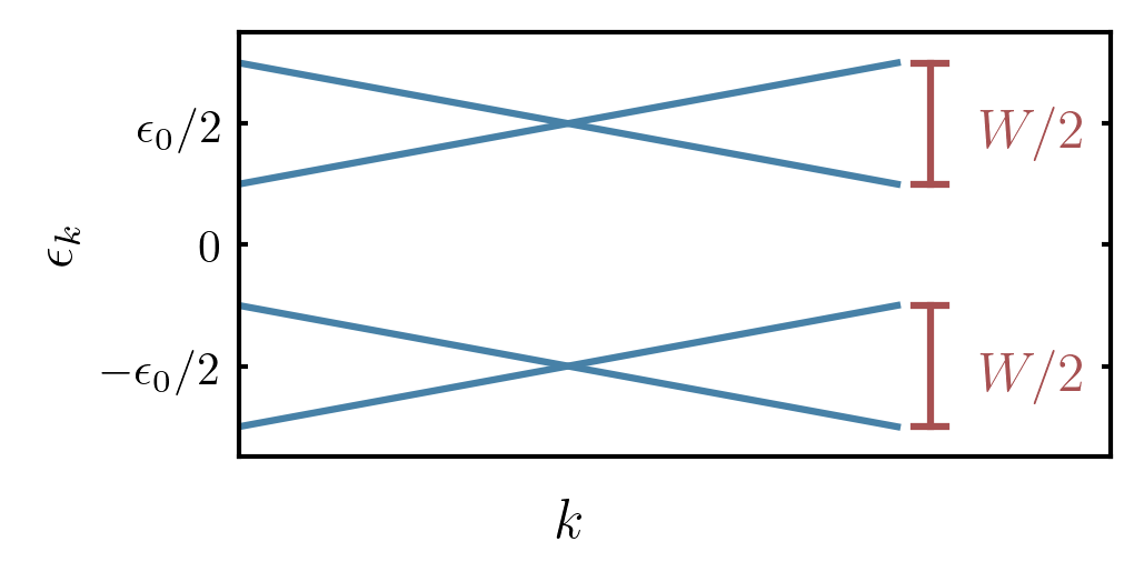
Figure 6: An example band structure with density of states matching the distribution of the inhomogeneous atomic energies shown in the left panel. In this diagram, $\epsilon_{0}>W/2$ such that there is a band gap of size $\epsilon_{0}-W/2$. Note that center of the bands are at $\pm\epsilon_{0}/2$ for the fermion band structure, and not $\pm\epsilon_{0}$ as for the atomic level distribution. This is because there are two fermions per cooper pair, and it is cooper pairs that map to atomic levels.

Appendix D Equilibrium Phase Diagram

While in the main text we consider quench dynamics from a state in which every possible Cooper pair is condensed, intuition about superconducting systems is often developed near thermal equilibrium. To make connection to that limit, we consider the superconducting order of the grand canonical state $\rho_{\mu,T}=\exp[-({H-2\mu(S^{z}+a^{\dagger}a)})/{K_{b}T}]$ with chemical potential $\mu$ and temperature $T\rightarrow 0$, and

$$H/\hbar=\sum_{i=1}^{2N}\epsilon_{i}\sigma^{z}_{i}+\sum_{i=1}^{2N}g_{i}(\sigma^{\dagger}_{i}a+h.c.)+\Delta_{c}a^{\dagger}a.$$ (13)

This model has a $U(1)$ symmetry generated by the conservation of total excitations $\sum_{i}\frac{1}{2}\sigma^{z}_{i}+n$. At high $T$ and $\mu=0$, the system enters a symmetric phase with $\left<\vec{\sigma}\right>\rightarrow 0$ and with photon occupation scaling monotonically with $K_{b}T$. At low temperature, a symmetric phase with all spins polarized on the $\hat{z}$ axis, $\left<\sigma^{z}_{i}\right>=\text{sign}(\epsilon_{i}-\mu)$ (a normal state insulator or conductor), competes with a symmetry broken phase can where $\left|\left<S^{+}\right>\right|>0$ and $\left<a\right>>0$. Away from the quantum critical point separating these two phases, a mean field approximation (i.e. $\left<O_{1}(t)O_{2}(t)\right>=\left<O_{1}(t)\right>\left<O_{2}(t)\right>$) is valid, and we again adopt the notation: $\left<O_{1}\right>\equiv O_{1}$. At zero temperature, energy is minimized at the fixed points of the classical dynamics, $\partial_{t}\vec{\sigma}=0$ and $\partial_{t}a=0$. The later condition fixes the photon in a way mathematically equivalent to the adiabatic condition:

$$a=-\frac{g}{\Delta_{c}-2\mu}\sum_{i}\sigma^{-}_{i}(t).$$ (14)

Defining the gap as $\Delta=\frac{g^{2}}{\Delta_{c}-2\mu}\sum_{i}\sigma^{+}_{i}$ and inserting Eq. 14 into Eq. 13, one finds that the spins minimize energy in an effective magnetic field $\vec{h}=(\epsilon_{i}-\mu)\hat{z}+\text{Re}(\Delta)\hat{x}+\text{Im}(\Delta)\hat{x}$. Minimizing the energy of the spins in this field we find:

$$\sigma^{+} = \frac{\Delta}{2\sqrt{(\epsilon_{i}-\mu)^{2}+\Delta^{2}}}$$ (15)

$$\sigma^{z}_{i} = \frac{\epsilon_{i}-\mu/2}{\sqrt{(\epsilon_{i}-\mu)^{2}+\Delta^{2}}}$$

using $g^{2}=\chi N\Delta_{c}$ we get the gap equation:

$$1=\frac{\chi N\Delta^{c}}{W(\Delta^{c}-2\mu)}\int_{\mathcal{R}}d\epsilon\frac{\Delta}{\sqrt{(\epsilon-\mu)^{2}+\Delta^{2}}}$$

where the integral is over the region defining the constant density of states: $\mathcal{R}=\epsilon\in(\epsilon_{0}/2-W/4,\epsilon_{0}/2-W/4)\cup(-\epsilon_{0}/2-W/4,-\epsilon_{0}/2-W/4)$. In addition to the gap equation, we can also restrict the total number of excitations to match that of the initial state in the paper:

$$a^{\dagger}a+S^{z}=0=\frac{N}{2W}\int_{\mathcal{R}}d\epsilon\frac{\epsilon-\mu}{\sqrt{(\epsilon-\mu)^{2}+\Delta^{2}}}+\frac{\Delta^{2}}{\chi\Delta_{c}}$$ (16)

In the adiabatic limit, $\Delta_{c}/(\chi N)\gg 1$, the photon amplitude goes to zero, and thus $S^{z}$ must also limit to zero. This is ensured by a chemical potential $\mu=0$ such that $\epsilon_{i}-\mu$ is positive for half the spins and negative for the other half. The resulting zero temperature phase diagram is calculated numerically and is shown in Fig. 7. At finite temperature, the superconducting coherence $\left|S^{+}\right|$ is reduced in the ordered phase and remains $0$ in the disordered phase. Weather the disordered phase is a insulator or conductor at low temperature depends on if the chemical potential $\mu=0$ is located in a band or band gap. Upon consideration of Fig. 6, we see the disordered phase is a two-band insulator when $\epsilon_{0}>W/2$ and a single band conductor for larger dispersion $W$. Upon inspection of Fig. 7, we see that for the adiabatic limit studied in the paper, the system would traditionally be considered a two-band insulator.

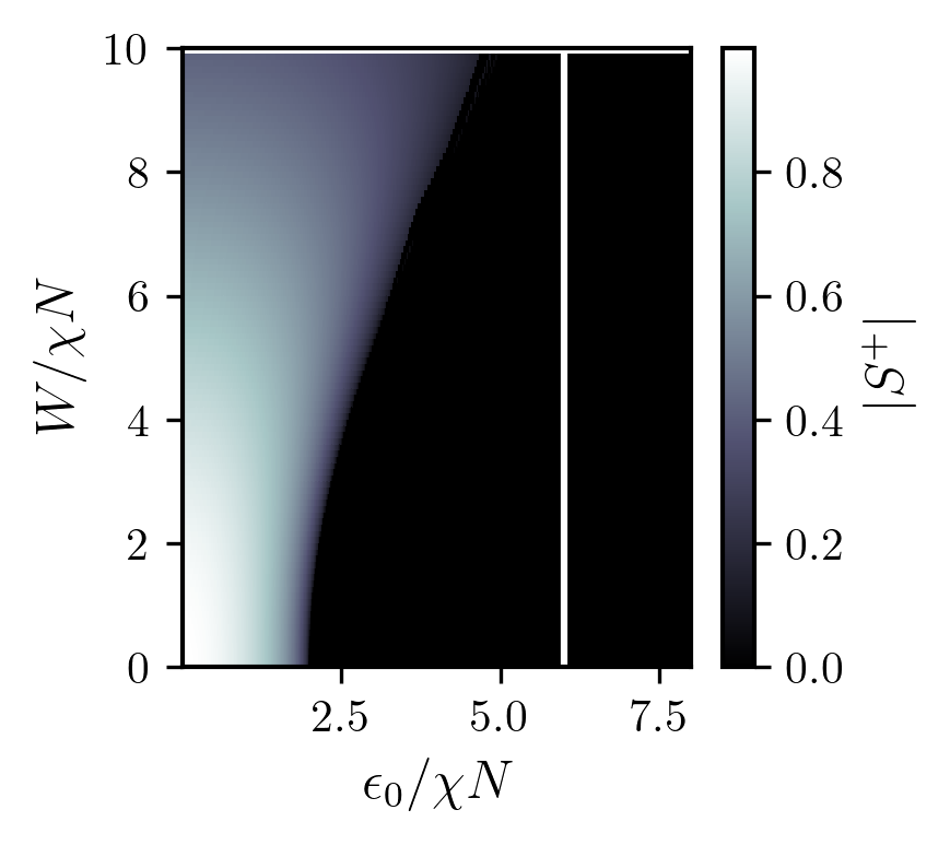
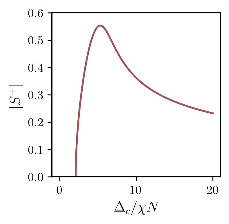
Figure 7: Left Panel: Equilibrium phase diagram at $T=0$ and with chemical potential fixed to $\mu=0$. In the paper we study the line along $\epsilon_{0}/\chi N=6$ which has $\left|S^{+}\right|=0$ in the ground state and at all finite temperatures. Right Panel: Zero temperature coherence, $S^{+}$, versus photon detuning, $\Delta_{c}/\chi N$, with $\mu$ chosen to fix the total number of excitations, $a^{\dagger}a+\frac{1}{2}\sum_{i}\sigma^{z}_{i}=0$. This panel is for, $\epsilon_{0}/\chi N=6$ and $W/\chi N=8$ as in the paper and shows a similar resonance peak.

The phase diagram shown in the left panel of Fig. 7 holds for all values of $\Delta_{c}/\chi N$ assuming the chemical potential is fixed to $\mu=0$. If, instead, $\mu$ is chosen to fix the total number of excitations, it will depend on the detuning of the photon since, in the ordered phase, the photon occupation increases monotonically with $\chi N/\Delta_{c}$. Therefore, to maintain a fixed number of total excitations, the chemical potential must increase to ensure a finite and negative $S^{z}=-a^{\dagger}a$. This can lead to instabilities and produce an ordered phase where there was none in the adiabatic limit. Fixing $a^{\dagger}a+\frac{1}{2}\sum_{i}\sigma_{i}^{z}=0$, we find a similar resonant order at zero temperature as was seen out-of-equilibrium (see right panel of Fig. 7). Note, such an equilibrium state is unlikely to be observed in the cavity QED system due to the effects of dissipation which lead to a disordered state with no photons in the cavity at long times.

Appendix E Lindblad Dynamics

In order to investigate the effect of photon loss, we study dynamics of the spin and cavity evolving under the Liouvillian with jump operator $L=\sqrt{\kappa/2}a$. In the Heisenberg picture operators evolve following

$$\partial_{t}O=i\left[H,O\right]+2L^{\dagger}OL-\left\{L^{\dagger}L,O\right\}$$ (17)

where $\kappa$ is the loss rate. In the mean field limit (i.e. $\left<O_{1}(t)O_{2}(t)\right>=\left<O_{1}(t)\right>\left<O_{2}(t)\right>$), we can truncate the hierarchy of equations generated by Eq. 17. We then numerically evolve the closed set of equations for the spin and photon variables.

References

- Ashcroft et al. (1976) Neil W Ashcroft, N David Mermin, et al., “Solid state physics,” (1976).
- Annett (2004) James F. Annett, Superconductivity, Superfluids and Condensates, Oxford Master Series in Physics (Oxford University Press, Oxford, New York, 2004).
- Varma et al. (1989) C. M. Varma, P. B. Littlewood, S. Schmitt-Rink, E. Abrahams, and A. E. Ruckenstein, “Phenomenology of the normal state of cu-o high-temperature superconductors,” Phys. Rev. Lett. 63, 1996–1999 (1989).
- Ginsberg (1998) Donald M Ginsberg, Physical properties of high temperature superconductors I (World scientific, 1998).
- Dagotto (1994) Elbio Dagotto, “Correlated electrons in high-temperature superconductors,” Rev. Mod. Phys. 66, 763–840 (1994).
- Matsunaga et al. (2013) Ryusuke Matsunaga, Yuki I Hamada, Kazumasa Makise, Yoshinori Uzawa, Hirotaka Terai, Zhen Wang, and Ryo Shimano, “Higgs amplitude mode in the bcs superconductors nb 1- x ti x n induced by terahertz pulse excitation,” Physical review letters 111, 057002 (2013).
- Matsunaga et al. (2014) Ryusuke Matsunaga, Naoto Tsuji, Hiroyuki Fujita, Arata Sugioka, Kazumasa Makise, Yoshinori Uzawa, Hirotaka Terai, Zhen Wang, Hideo Aoki, and Ryo Shimano, “Light-induced collective pseudospin precession resonating with higgs mode in a superconductor,” Science 345, 1145–1149 (2014).
- Mankowsky et al. (2014) Roman Mankowsky, Alaska Subedi, Michael Först, Simon O Mariager, Matthieu Chollet, HT Lemke, Jeffrey S Robinson, James M Glownia, Michael P Minitti, Alex Frano, et al., “Nonlinear lattice dynamics as a basis for enhanced superconductivity in yba 2 cu 3 o 6.5,” Nature 516, 71–73 (2014).
- Mitrano et al. (2016) Matteo Mitrano, Alice Cantaluppi, Daniele Nicoletti, Stefan Kaiser, A Perucchi, S Lupi, P Di Pietro, D Pontiroli, M Riccò, Stephen R Clark, et al., “Possible light-induced superconductivity in k 3 c 60 at high temperature,” Nature 530, 461–464 (2016).
- Isoyama et al. (2021) Kazuki Isoyama, Naotaka Yoshikawa, Kota Katsumi, Jeremy Wong, Naoki Shikama, Yuki Sakishita, Fuyuki Nabeshima, Atsutaka Maeda, and Ryo Shimano, “Light-induced enhancement of superconductivity in iron-based superconductor fese0. 5te0. 5,” Communications Physics 4, 1–9 (2021).
- Curtis et al. (2019) Jonathan B Curtis, Zachary M Raines, Andrew A Allocca, Mohammad Hafezi, and Victor M Galitski, “Cavity quantum eliashberg enhancement of superconductivity,” Physical review letters 122, 167002 (2019).
- Schlawin and Jaksch (2019) Frank Schlawin and Dieter Jaksch, “Cavity-mediated unconventional pairing in ultracold fermionic atoms,” Physical review letters 123, 133601 (2019).
- Chakraborty and Piazza (2020) Ahana Chakraborty and Francesco Piazza, “Non-bcs-type enhancement of superconductivity from long-range photon fluctuations,” arXiv preprint arXiv:2008.06513 (2020).
- Sentef et al. (2018) Michael A Sentef, Michael Ruggenthaler, and Angel Rubio, “Cavity quantum-electrodynamical polaritonically enhanced electron-phonon coupling and its influence on superconductivity,” Science advances 4, eaau6969 (2018).
- Thomas et al. (2019) Anoop Thomas, Eloïse Devaux, Kalaivanan Nagarajan, Thibault Chervy, Marcus Seidel, David Hagenmüller, Stefan Schütz, Johannes Schachenmayer, Cyriaque Genet, Guido Pupillo, et al., “Exploring superconductivity under strong coupling with the vacuum electromagnetic field,” arXiv preprint arXiv:1911.01459 (2019).
- Laussy et al. (2010) Fabrice P Laussy, Alexey V Kavokin, and Ivan A Shelykh, “Exciton-polariton mediated superconductivity,” Physical review letters 104, 106402 (2010).
- Cotleţ et al. (2016) Ovidiu Cotleţ, Sina Zeytino?lu, Manfred Sigrist, Eugene Demler, and Ataç Imamo?lu, “Superconductivity and other collective phenomena in a hybrid bose-fermi mixture formed by a polariton condensate and an electron system in two dimensions,” Physical Review B 93, 054510 (2016).
- Smolka et al. (2014) Stephan Smolka, Wolf Wuester, Florian Haupt, Stefan Faelt, Werner Wegscheider, and Ataç Imamoglu, “Cavity quantum electrodynamics with many-body states of a two-dimensional electron gas,” Science 346, 332–335 (2014).
- Mazza and Georges (2019) Giacomo Mazza and Antoine Georges, “Superradiant quantum materials,” Physical review letters 122, 017401 (2019).
- Andolina et al. (2019) GM Andolina, FMD Pellegrino, V Giovannetti, AH MacDonald, and M Polini, “Cavity quantum electrodynamics of strongly correlated electron systems: A no-go theorem for photon condensation,” Physical Review B 100, 121109 (2019).
- Kiffner et al. (2019) Martin Kiffner, Jonathan R Coulthard, Frank Schlawin, Arzhang Ardavan, and Dieter Jaksch, “Manipulating quantum materials with quantum light,” Physical Review B 99, 085116 (2019).
- Latini et al. (2019) Simone Latini, Enrico Ronca, Umberto De Giovannini, Hannes Hübener, and Angel Rubio, “Cavity control of excitons in two-dimensional materials,” Nano letters 19, 3473–3479 (2019).
- Li et al. (2020) Jiajun Li, Denis Golez, Giacomo Mazza, Andrew J Millis, Antoine Georges, and Martin Eckstein, “Electromagnetic coupling in tight-binding models for strongly correlated light and matter,” Physical Review B 101, 205140 (2020).
- Ashida et al. (2020) Yuto Ashida, Ataç İmamoğlu, Jérôme Faist, Dieter Jaksch, Andrea Cavalleri, and Eugene Demler, “Quantum electrodynamic control of matter: Cavity-enhanced ferroelectric phase transition,” Physical Review X 10, 041027 (2020).
- Gao et al. (2020) Hongmin Gao, Frank Schlawin, Michele Buzzi, Andrea Cavalleri, and Dieter Jaksch, “Photoinduced electron pairing in a driven cavity,” Physical Review Letters 125, 053602 (2020).
- Garcia-Vidal et al. (2021) Francisco J Garcia-Vidal, Cristiano Ciuti, and Thomas W Ebbesen, “Manipulating matter by strong coupling to vacuum fields,” Science 373, eabd0336 (2021).
- Hübener et al. (2021) Hannes Hübener, Umberto De Giovannini, Christian Schäfer, Johan Andberger, Michael Ruggenthaler, Jerome Faist, and Angel Rubio, “Engineering quantum materials with chiral optical cavities,” Nature materials 20, 438–442 (2021).
- Li and Eckstein (2020) Jiajun Li and Martin Eckstein, “Manipulating intertwined orders in solids with quantum light,” Physical Review Letters 125, 217402 (2020).
- Lenk and Eckstein (2020) Katharina Lenk and Martin Eckstein, “Collective excitations of the u (1)-symmetric exciton insulator in a cavity,” Physical Review B 102, 205129 (2020).
- Chiocchetta et al. (2021) Alessio Chiocchetta, Dominik Kiese, Carl Philipp Zelle, Francesco Piazza, and Sebastian Diehl, “Cavity-induced quantum spin liquids,” Nature Communications 12, 1–8 (2021).
- Ashida et al. (2021) Yuto Ashida, Ataç İmamoğlu, and Eugene Demler, “Cavity quantum electrodynamics at arbitrary light-matter coupling strengths,” Physical Review Letters 126, 153603 (2021).
- Raines et al. (2020) Zachary M Raines, Andrew A Allocca, Mohammad Hafezi, and Victor M Galitski, “Cavity higgs polaritons,” Physical Review Research 2, 013143 (2020).
- Gao et al. (2021) Hongmin Gao, Frank Schlawin, and Dieter Jaksch, “Higgs mode stabilization by photo-induced long-range interactions in a superconductor,” arXiv preprint arXiv:2106.05076 (2021).
- Smale et al. (2019) Scott Smale, Peiru He, Ben A Olsen, Kenneth G Jackson, Haille Sharum, Stefan Trotzky, Jamir Marino, Ana Maria Rey, and Joseph H Thywissen, “Observation of a transition between dynamical phases in a quantum degenerate fermi gas,” Science advances 5, eaax1568 (2019).
- Lewis-Swan et al. (2021) Robert J. Lewis-Swan, Diego Barberena, Julia R. K. Cline, Dylan J. Young, James K. Thompson, and Ana Maria Rey, “Cavity-QED Quantum Simulator of Dynamical Phases of a Bardeen-Cooper-Schrieffer Superconductor,” Phys. Rev. Lett. 126, 173601 (2021).
- Agarwal et al. (1997) G. S. Agarwal, R. R. Puri, and R. P. Singh, “Atomic Schrödinger cat states,” Phys. Rev. A 56, 2249–2254 (1997).
- Damanet et al. (2019) François Damanet, Andrew J. Daley, and Jonathan Keeling, “Atom-only descriptions of the driven-dissipative Dicke model,” Phys. Rev. A 99, 033845 (2019).
- Kelly et al. (2021) Shane P. Kelly, Ana Maria Rey, and Jamir Marino, “Effect of active photons on dynamical frustration in cavity qed,” Phys. Rev. Lett. 126, 133603 (2021).
- Muniz et al. (2020) Juan A. Muniz, Diego Barberena, Robert J. Lewis-Swan, Dylan J. Young, Julia R. K. Cline, Ana Maria Rey, and James K. Thompson, “Exploring dynamical phase transitions with cold atoms in an optical cavity,” Nature 580, 602–607 (2020).
- Norcia et al. (2018) Matthew A. Norcia, Robert J. Lewis-Swan, Julia R. K. Cline, Bihui Zhu, Ana M. Rey, and James K. Thompson, “Cavity-mediated collective spin-exchange interactions in a strontium superradiant laser,” Science 361, 259–262 (2018).
- Palacino and Keeling (2020) Roberta Palacino and Jonathan Keeling, “Atom-only theories for U(1) symmetric cavity-QED models,” arXiv:2011.12120 [cond-mat, physics:quant-ph] (2020), arXiv:2011.12120 [cond-mat, physics:quant-ph] .
- Davis et al. (2019) Emily J. Davis, Gregory Bentsen, Lukas Homeier, Tracy Li, and Monika H. Schleier-Smith, “Photon-mediated spin-exchange dynamics of spin-1 atoms,” Phys. Rev. Lett. 122, 010405 (2019).
- Periwal et al. (2021) Avikar Periwal, Eric S Cooper, Philipp Kunkel, Julian F Wienand, Emily J Davis, and Monika Schleier-Smith, “Programmable interactions and emergent geometry in an atomic array,” arXiv preprint arXiv:2106.04070 (2021).
- Vaidya et al. (2018) Varun D. Vaidya, Yudan Guo, Ronen M. Kroeze, Kyle E. Ballantine, Alicia J. Kollár, Jonathan Keeling, and Benjamin L. Lev, “Tunable-range, photon-mediated atomic interactions in multimode cavity qed,” Phys. Rev. X 8, 011002 (2018).
- Marsh et al. (2021) Brendan P. Marsh, Yudan Guo, Ronen M. Kroeze, Sarang Gopalakrishnan, Surya Ganguli, Jonathan Keeling, and Benjamin L. Lev, “Enhancing associative memory recall and storage capacity using confocal cavity qed,” Phys. Rev. X 11, 021048 (2021).
- Seetharam et al. (2021) Kushal Seetharam, Alessio Lerose, Rosario Fazio, and Jamir Marino, “Correlation engineering via non-local dissipation,” arXiv preprint arXiv:2101.06445 (2021).
- Klinder et al. (2015) Jens Klinder, Hans Keßler, Matthias Wolke, Ludwig Mathey, and Andreas Hemmerich, “Dynamical phase transition in the open dicke model,” Proceedings of the National Academy of Sciences 112, 3290–3295 (2015).
- Mivehvar et al. (2021) Farokh Mivehvar, Francesco Piazza, Tobias Donner, and Helmut Ritsch, “Cavity qed with quantum gases: New paradigms in many-body physics,” arXiv preprint arXiv:2102.04473 (2021).
- Baumann et al. (2010) Kristian Baumann, Christine Guerlin, Ferdinand Brennecke, and Tilman Esslinger, “Dicke quantum phase transition with a superfluid gas in an optical cavity,” nature 464, 1301–1306 (2010).
- Brennecke et al. (2007) Ferdinand Brennecke, Tobias Donner, Stephan Ritter, Thomas Bourdel, Michael Köhl, and Tilman Esslinger, “Cavity qed with a bose–einstein condensate,” nature 450, 268–271 (2007).
- Fogarty et al. (2015) T. Fogarty, C. Cormick, H. Landa, Vladimir M. Stojanović, E. Demler, and Giovanna Morigi, “Nanofriction in Cavity Quantum Electrodynamics,” Phys. Rev. Lett. 115, 233602 (2015).
- Habibian et al. (2013) Hessam Habibian, André Winter, Simone Paganelli, Heiko Rieger, and Giovanna Morigi, “Bose-Glass Phases of Ultracold Atoms due to Cavity Backaction,” Phys. Rev. Lett. 110, 075304 (2013).
- Himbert et al. (2019) Lukas Himbert, Cecilia Cormick, Rebecca Kraus, Shraddha Sharma, and Giovanna Morigi, “Mean-field phase diagram of the extended Bose-Hubbard model of many-body cavity quantum electrodynamics,” Phys. Rev. A 99, 043633 (2019).
- Keller et al. (2018) Tim Keller, Valentin Torggler, Simon B Jäger, Stefan Schütz, Helmut Ritsch, and Giovanna Morigi, “Quenches across the self-organization transition in multimode cavities,” New Journal of Physics 20, 025004 (2018).
- Keller et al. (2017) Tim Keller, Simon B Jäger, and Giovanna Morigi, “Phases of cold atoms interacting via photon-mediated long-range forces,” Journal of Statistical Mechanics: Theory and Experiment 2017, 064002 (2017).
- Schütz et al. (2016) Stefan Schütz, Simon B. Jäger, and Giovanna Morigi, “Dissipation-assisted prethermalization in long-range interacting atomic ensembles,” Phys. Rev. Lett. 117, 083001 (2016).
- Xu et al. (2016) Minghui Xu, Simon B. Jäger, S. Schütz, J. Cooper, Giovanna Morigi, and M. J. Holland, “Supercooling of atoms in an optical resonator,” Phys. Rev. Lett. 116, 153002 (2016).
- Yuzbashyan et al. (2015) E. A. Yuzbashyan, M. Dzero, V. Gurarie, and M. S. Foster, “Quantum quench phase diagrams of an s-wave BCS-BEC condensate,” Phys. Rev. A 91, 033628 (2015).
- Dukelsky et al. (2004a) J. Dukelsky, S. Pittel, and G. Sierra, “Colloquium: Exactly solvable Richardson-Gaudin models for many-body quantum systems,” Rev. Mod. Phys. 76, 643–662 (2004a).
- Richardson (2002) R. W. Richardson, “New Class of Solvable and Integrable Many-Body Models,” arXiv:cond-mat/0203512 (2002), arXiv:cond-mat/0203512 .
- Barankov and Levitov (2006) R. A. Barankov and L. S. Levitov, “Synchronization in the bcs pairing dynamics as a critical phenomenon,” Phys. Rev. Lett. 96, 230403 (2006).
- Barankov et al. (2004) RA Barankov, LS Levitov, and BZ Spivak, “Collective rabi oscillations and solitons in a time-dependent bcs pairing problem,” Physical review letters 93, 160401 (2004).
- Yuzbashyan et al. (2005a) Emil A. Yuzbashyan, Boris L. Altshuler, Vadim B. Kuznetsov, and Victor Z. Enolskii, “Nonequilibrium Cooper pairing in the nonadiabatic regime,” Phys. Rev. B 72, 220503 (2005a).
- Yuzbashyan et al. (2005b) Emil A. Yuzbashyan, Boris L. Altshuler, Vadim B. Kuznetsov, and Victor Z. Enolskii, “Solution for the dynamics of the BCS and central spin problems,” J. Phys. A: Math. Gen. 38, 7831–7849 (2005b).
- Yuzbashyan et al. (2006) Emil A. Yuzbashyan, Oleksandr Tsyplyatyev, and Boris L. Altshuler, “Relaxation and Persistent Oscillations of the Order Parameter in Fermionic Condensates,” Phys. Rev. Lett. 96, 097005 (2006).
- Norcia and Thompson (2016) Matthew A. Norcia and James K. Thompson, “Cold-strontium laser in the superradiant crossover regime,” Phys. Rev. X 6, 011025 (2016).
- Note (1) See SM for band structure and equilibrium phase diagram.
- Kirton and Keeling (2017) Peter Kirton and Jonathan Keeling, “Suppressing and Restoring the Dicke Superradiance Transition by Dephasing and Decay,” Phys. Rev. Lett. 118, 123602 (2017).
- Kirton and Keeling (2018) Peter Kirton and Jonathan Keeling, “Superradiant and lasing states in driven-dissipative Dicke models,” New J. Phys. 20, 015009 (2018).
- Kirton et al. (2019) Peter Kirton, Mor M. Roses, Jonathan Keeling, and Emanuele G. Dalla Torre, “Introduction to the Dicke Model: From Equilibrium to Nonequilibrium, and Vice Versa,” Advanced Quantum Technologies 2, 1800043 (2019).
- Dukelsky et al. (2004b) J. Dukelsky, S. Pittel, and G. Sierra, “Colloquium: Exactly solvable richardson-gaudin models for many-body quantum systems,” Rev. Mod. Phys. 76, 643–662 (2004b).
- Richardson and Sherman (1964) R.W. Richardson and N. Sherman, “Exact eigenstates of the pairing-force hamiltonian,” Nuclear Physics 52, 221–238 (1964).
- Gaudin (1976) M. Gaudin, “Diagonalisation d’une classe d’hamiltoniens de spin,” Journal de Physique 37, 1087–1098 (1976).
- Note (2) See SM for details on Lax Analysis.
- Note (4) See SM for the relation between resonance and minimum of photon density.
- Note (3) See SM for details on mean field approximation for Lindblad Evolution.
- Bruzewicz et al. (2019) Colin D. Bruzewicz, John Chiaverini, Robert McConnell, and Jeremy M. Sage, “Trapped-ion quantum computing: Progress and challenges,” Applied Physics Reviews 6, 021314 (2019).
- Chang et al. (2018) D. E. Chang, J. S. Douglas, A. González-Tudela, C.-L. Hung, and H. J. Kimble, “Colloquium: Quantum matter built from nanoscopic lattices of atoms and photons,” Rev. Mod. Phys. 90, 031002 (2018).