Fast Model-based Policy Search for Universal Policy Networks

Abstract

Adapting an agent’s behaviour to new environments has been one of the primary focus areas of physics based reinforcement learning. Although recent approaches such as universal policy networks partially address this issue by enabling the storage of multiple policies trained in simulation on a wide range of dynamic/latent factors, efficiently identifying the most appropriate policy for a given environment remains a challenge. In this work, we propose a Gaussian Process-based prior learned in simulation, that captures the likely performance of a policy when transferred to a previously unseen environment. We integrate this prior with a Bayesian Optimisation-based policy search process to improve the efficiency of identifying the most appropriate policy from the universal policy network. We empirically evaluate our approach in a range of continuous and discrete control environments, and show that it outperforms other competing baselines.

I Introduction

Over the last decade, deep reinforcement learning (RL) agents have achieved a number of milestones such as matching and exceeding human level performances in games such as Go [1] and Atari [2]. However, their poor sample efficiency is a major impediment to real-world applications where it is impractical to collect millions of training samples [2]. For physics-based tasks such as robotics, numerical simulators based on known laws of physics can be used as a cheap surrogate of the real-world. However, such simulators often have many simulation parameters, usually representing real-world latent factors such as mass, friction etc., which need to be estimated (i.e. system identification) before the simulator can be used for learning.

A common approach to this problem is estimating parameters from trajectory observations (sequence of states for a fixed duration of time) in the real world by minimising the difference between simulated and real world trajectories [3, 4, 5, 6, 7]. However, these works are focussed on grounding the system as a whole, i.e., estimating all the simulation parameters without considering the downstream task. In most situations, not all parameters are important for a given task. For example, in basketball, bounciness of the ball is likely to be more relevant in comparison to surface friction, whereas in ten-pin bowling, the reverse is true. Thus, in situations where the task specification is available, spending samples to estimate all the parameters accurately (i.e. ‘full grounding’) may be completely unnecessary.

Domain Randomisation [8, 9] proposes to find a task-specific but environment-independent robust policy across a wide range of values of the simulation parameters. But in practice this approach has been shown to produce overly conservative policies, especially if dynamics vary considerably across the full range of parameters [10]. A more useful line of research that utilises task-specific knowledge to only ‘partially ground’ the system relies on training a Universal Policy Network (UPN) [11] modelled through a large deep model and trained across a range of parameter values. These models are capable of producing environment specific policies when conditioned through the corresponding environment parameters. The system identification is performed by trying out different sets of parameter values, rolling out the corresponding UPN policies in the real environment (i.e., transfer performance) and finding the parameter set that maximises the reward [12]. This can be performed by any efficient optimiser such as Bayesian optimisation (BO) [13]. Partial grounding happens automatically as the optimiser progressively identifies the influence of individual parameters and use that knowledge in the optimisation. However, current BO-based approaches start with no prior knowledge of the task and thus lack the power to exploit any intrinsic relations between different policies for improved sample-efficiency.

With this motivation, we first propose a ‘self-play’-like approach where we evaluate the performance of the UPN policies individually across different values of parameters and build prior knowledge on the inter-policy relationships, all within the simulation environment. We discovered that (a) in many tasks, some policies are universally good, i.e., using that policy across a range of parameters often produces similarly good rewards, and (b) there exist policies that perform well only for a narrow range of parameters. Such knowledge, especially the existence of universally good policies can make policy search easier and efficient. We then encode such knowledge in BO via a transfer learning method to further accelerate the BO-based policy search approach [14]. Specifically, we discretize the parameter values, and at each sampled point we gather the set of simulated performance values by rolling out its UPN policy at different parameter regimes in the simulator. We then create a synthetic performance observation at that sampled point by assuming the observation to be Gaussian with mean and variance calculated from the set of the simulated performance values. If the samples do not follow a Gaussian distribution, the observation is dropped. This ensures that the prior observations are consistent with the Gaussian process (GP) that is used as the main probabilistic model for BO. Next, we use the transfer learning method in [14] to treat these synthetic observations as source observations and create a GP that inherits the rich knowledge from this source data. Using the method enables our approach to be no worse in convergence than standard BO without any prior observations. We observe that such acceleration in BO produces much faster policy identification than the vanilla BO approach. We evaluate our approach in three MuJoCo tasks[15] and two contextual bandit scenarios, PHYRE [16] and our own Basketball environment, and observe that our method can produce significant improvements over state-of-the-art methods. In short, our contributions are:

1. Proposing a conceptual framework using inter-policy relationship for accelerating policy search on Universal Policy Network based simulator-in-the-loop learning.

2. Deriving a transfer learning-based Bayesian optimisation method to exploit the inter-policy relationship in a principled way.

3. Demonstration of the the benefit of our approach on a set of physics tasks from both contextual bandit and classic RL settings.

Although we have proposed our approach for physics based RL settings, we believe it can be adapted to any parameterisable environment where the parameters are not necessarily physical, but still influences the dynamics of the environment e.g., skill of another agent in the same environment, user preferences for recommendations, etc. Thus, we see a broader impact of our work in areas beyond physics based RL settings.

II Methodology

In this work, we propose a simulator-in-the-loop learning algorithm that requires minimal interaction with the real world for policy learning in an RL setting.

To achieve this we adopt an RL approach commonly referred to as Universal Policy Networks (UPN), that makes it practical to store and evaluate a large collection of policies for different latent factors (e.g. mass, friction) without having to re-train the agents for each latent factor combination. We train the UPN as an RL agent, for which we formalise the learning problem as a Markov Decision Process (MDP). The MDP is represented as a tuple of $<\mathcal{S},\mathcal{A},\mathcal{T},\theta,\mathcal{R}>$, where $\mathcal{S}$ is the state space, $\mathcal{A}$ is the action space and $\theta$ is the set of latent factors. Furthermore, $\mathcal{T}:\mathcal{S}\times\mathcal{A}\times\theta\rightarrow\mathcal{S}$ is the transition function, and $\mathcal{R}:\mathcal{S}\times\mathcal{A}\rightarrow\mathbb{R}$ is the reward function. UPN’s state is constructed by combining the task’s observable state (e.g. object positions and velocity) and true latent factors (e.g. friction), which makes it possible for an RL algorithm to learn policies over different latent factors and often seamlessly generalise them to unseen latent factors if the policy space is smooth with respect to the latent parameters.

In our problem setup, we consider a real world environment $\psi_{r}$, and assume the availability of a corresponding simulated environment $\psi$. We assume these environments are governed by transition functions $\mathcal{T}_{r}$ and $\mathcal{T}_{s}$ respectively, that differ in their respective latent factors $\Theta$ and $\theta$ ($\Theta,\theta\in\mathbb{R}^{d}$). $\Theta$, associated with the real environment is given by $\Theta=\theta_{r}+\epsilon$ where $\theta_{r}\in\mathbb{R}^{d}$ represents some unknown, but modelable, fixed latent factor value and $\epsilon\in\mathbb{R}^{d}$ represents some unmodellable dynamics (e.g. air resistance). The transition function $\mathcal{T}_{s}$ of the simulated environment $\psi$ can be controlled through its latent factors $\theta$.

Our aim is to maximise performance on a real world task set $W$ with a fixed reward function, by efficiently learning a policy $\pi$ through minimal interactions with the real-world. To achieve this objective, we aim to learn a sufficiently good value of $\theta$ to the extent that $\pi$ trained on dynamics $\mathcal{T}_{s}$ would return a relatively high performance when evaluated on $W$ with dynamics $\mathcal{T}_{r}$. For this purpose, we evaluate $T$ policies $\pi_{n=1,..,T}$ fetched (i.e. conditioned) from the UPN at different $\theta$, on $W$. We refer to this process as policy search where the sequence of $\pi_{n}$ is constructed by Bayesian Optimisation (BO) for discovering the optimal policy within a small value of $T$. To perform policy search with a reduced number of interactions with the real-world, we integrate a prior constructed by evaluating the goodness of $\pi$ over a range of $\theta$. We call this prior Policy prior.

The overall design of our approach consists of two components. 1) a UPN based Policy Search; and 2) Policy prior incorporated into the BO based latent factor estimation process (Figure 1). These components are discussed in the following sections:

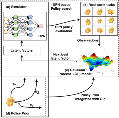
Figure 1: A sample efficient online system identification workflow using a universal policy network (UPN) based policy search and Policy Prior. (a) The latent factor conditioned policy from UPN is (b) transferred to a set of real-world tasks, and (c) evaluations are fed as observations to a GP model. GP is used as part of BO based policy search. (d) To improve GP model’s sample efficiency, we integrate Policy Prior which is the simulated prior generated by rolling out a task policy in $e_{1},..,e_{E}$ environment settings with different latent factors.

II-A UPN Based Policy Search

To formulate the UPN, we augment the task’s state $s_{t}\in S$ as $s_{t}=[o_{t},\theta]$, where $o_{t}$ is the task’s observable state at time step $t$, and $\theta$ is the set of latent factors for the given episode (we assume, $\theta$ is fixed for a given episode throughout this study). Even though UPNs have been implemented with policy gradient algorithms for mainly continuous action tasks [17, 18], in this study we also design a DQN based UPN for discrete action tasks such as bandit tasks. However, to examine the performance of Policy prior for continuous action tasks, we adopt the existing policy gradient based UPN. When training the UPN, we only use simulation, making it inexpensive and practical.

Once we obtain a trained UPN, when conditioned by the latent factor estimate $\theta,$ it will produce a policy $\pi(s_{t}=[o_{t},\theta])$ for the time step $t$. We then evaluate this policy on the real-world task set $W$, and measure its performance (episodic return) $G_{W}(\pi)$. We use this measure as the optimisation objective for BO to find $\theta^{*}$ such that,

$$\theta^{*}=\underset{\theta}{argmax}\>G_{W}(\pi(s_{t}))\;\mid s_{t}=[o_{t},\theta]$$ (1)

II-B Policy Prior

To build the Policy prior, we first uniformly sample $N$ latent factors and retrieve policies $\pi_{n=1,..,N}$ for each corresponding $X_{n=1,..N}$ latent factors by concatenating $X_{n}$ with task observation state at the given time-step and using this augmented state to fetch a policy from the UPN (i.e., conditioning). Secondly, we define an environment setting $e$ as a simulation setting with some fixed latent factor configuration (i.e., $\psi_{\theta}$ for some $\theta$), and we select a set of uniformly sampled environment settings $E$ with $e\in E$ from defined bounds for the latent factors. To get a measure of the behaviour of $\pi_{n=1..N}$ policies in these $E$ settings, we evaluate each of $\pi_{n}$ on all $E$ simulated settings and record their performances. Subsequently, we calculate the distribution statistics, mean $\mu_{n=1,..,N}$ and variance $\sigma_{n=1,..,N}^{2}$ of jump starts for $E$ evaluations of each $\pi_{n}$.

Algorithm 1 Policy Prior Formation $(policy\_prior)$

Input:

1:$U$ - a simulator trained Universal Policy Network

2:$\xi\in W$ - a set of tasks

3:$\psi$ - a simulated environment

4:$N$ - Number of observations to sample

5:$e\in E$ - Environment settings with different ground truth latent values

6:$B_{l}$ - Bounds for latent factors $l$, $l\in\{1..L\}$

7:$\gamma$ - Minimum threshold of P-value for Gaussianity of sampled points

8:Output: $X_{1..N}$ latent factor samples, $\mu_{1,..N}$, $\sigma^{2}_{1,..N}$ mean and variance of UPN policies evaluated in $E$ environments

9://Sample latent values

10:for $l\leftarrow 1$ to $L$ do

11:     $X_{l}\leftarrow$ Generate $N$ uniform distributed observations in range $B_{l}$

12:end for

13://Evaluate sampled latent values across environments

14:for $n\leftarrow 1$ to $N$ do

15:     $\pi_{n}\leftarrow U$ conditioned policy at $X_{n}$

16:     for $e\leftarrow 1$ to $E$ do

17:         $Y_{n,e}\leftarrow$ $\pi_{n}$ evaluated in setting $e$ of simulator $\psi$ on task set $W$

18:     end for

19:     $\mu_{n}\leftarrow mean(Y_{n,1..E})$

20:     $\sigma^{2}_{n}\leftarrow variance(Y_{n,1..E})$

21:     //Call Kolmogorov-Smirnov test function [19] to calculate the p-value of $X_{n}$ sample for Gaussianity check. Sec. II-B1

22:     $p\_val_{n}=kstest(Y_{n,e=1..E},\mu_{n},\sigma^{2}_{n})$

23:     if $p\_val_{n}<\gamma$ then

24:         Remove $X_{n}$

25:     end if

26:end for

Algorithm 2 Physics aware BO Policy Search

Input:

1:$T$ - Number of BO iterations to run, $k$ - GP kernel, $\phi$ - GP initial hyperparameters, $\alpha$ - acquisition function, $\psi_{r}$ - real world, $W$ - task set to evaluate

2:Output: $x^{*}_{i=1..T}$, $y^{*}_{i=1..T}$ BO estimated new latent factors and corresponding real-world jump start performances

3:

4://Get Policy prior latent samples, mean and variance

5:$X_{1..N}$, $\mu_{1..N},\sigma^{2}_{1..N}\leftarrow policy\_prior$

6://Construct covariance matrix using kernel k

7:$K\leftarrow k(X_{1..N},X_{1..N};\phi)$

8://Add Policy prior variance as noise variance to Kernel matrix diagonal entries + $\epsilon$ sim-to-real noise. Eq. 2.

9:for $i\leftarrow 1$ to $N$ do $K_{i,i}\leftarrow K_{i,i}+\sigma^{2}_{i}+\epsilon$

10:end for

11://Build the Policy prior integrated Gaussian process

12:$GP_{p}\leftarrow GP(\mu_{1..N},K)$

13://Run the BO policy search for T iterations

14:for $i\leftarrow 1$ to $T$ do

15:     //acquisition function provides the next most likely latent factors to improve the optimisation objective

16:     $x^{*}_{i}\leftarrow\alpha(GP_{p})$

17:     // UPN conditioned policy at the latent factors suggested by acquisition function

18:     $\pi_{i}\leftarrow$ $U$ conditioned by $x^{*}_{i}$

19:     $y^{*}_{i}\leftarrow$ $\pi_{i}$ evaluated on task set $W$ in real-world $\psi_{r}$

20:     $GP_{p}\leftarrow GP_{p}\cup(x^{*}_{i},y^{*}_{i})$

21:end for

II-B1 Checking for Gaussianity of Prior

In the BO process, a Gaussian process is used as the model of the function. As per the modelling assumption of the Gaussian process, each observation should strictly follow a Gaussian distribution. Any mismatch between this assumption and reality will make the resultant model inconsistent and BO can get affected. Therefore, as an additional step, we verify whether the prior is distributed normally using Kolmogorov-Smirnov Goodness-of-Fit Test [20]. For this purpose, we iterate through all sampled latent values in the Policy prior to verify whether their p-values are within a defined threshold, and if they are not, the respective points are dropped from the prior.

II-B2 Knowledge Transfer with BO

To use these synthetic experiences as prior observations in the GP and then use it in the BO process we use the transfer BO algorithm of [14]. In [14], the transfer was done from a set of source observations to a target optimization problem. In our case, the source observations are the synthetic observations and the target observations come from the given real-world environment. With that, the synthetic observations now can be included just as a set of extra observations with added noise. The noise allows the GP to adjust for the expected difference of performance in the real-world, compared to the simulation world. This prior augmented GP’s observation data at time $t$ of the optimization can be denoted as $D_{t}$ = $\{X_{n},\mu_{n},\sigma^{2}_{n}\}_{n=1}^{N}\cup\{X_{i}^{*},y_{i}^{*}\}_{i=1}^{t}$, where $\{X_{i}^{*},y_{i}^{*}\}$ are real-world observations. This results in the kernel matrix form as:

$$K_{*}=K+\begin{bmatrix}\begin{bmatrix}\sigma_{1}&&0\\ &..\\ 0&&\sigma_{N}\end{bmatrix}_{N\times N}\\ &\sigma_{r}^{2}I_{t\times t}\end{bmatrix}$$ (2)

where $K$ is the covariance matrix for $\{X_{n=1}^{N}\cup X^{*}_{i=1..t}\}$, and $\sigma^{2}_{r}\in\mathbb{R}$ is the noise variance for real-world observations.

The posterior is computed based on this $K_{*}$ and $D_{t}$. We choose this transfer learning BO algorithm because of its favourable convergence property that shows the convergence is no worse than a standard BO without prior observations (3.1, Theorem 2 of [14]).

The process of building Policy prior is detailed in Algorithm 1, while the overall Policy prior integrated BO policy search is explained in Algorithm 2.

III Experiments

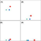
(a) Bowling - keep the green and blue balls in contact

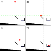
(b) Basketball - throw the ball into the basket using a plank

Figure 2: Evaluated contextual bandit tasks. a) Green and blue balls are initialised with different locations and sizes. An agent can choose the position (x, y coordinates) and the radius of the red ball with the aim of keeping the blue and green balls in contact for 3 seconds. b) The ball and the plank (fixed at 45 degree angle) need to be positioned so that the ball bounces into the basket. The plank position is constrained to be below the horizontal green line and to the left of the vertical gray line.

III-A Experiment setup

To demonstrate our approach, we consider a range of physics-based tasks - two contextual bandit tasks and three continuous control RL tasks. For continuous control tasks, we adopt three MuJoCo tasks: Half Cheetah-v1, Hopper-v1 and Walker2D-v1 [15], implemented using MuJuCo physics simulator [21]. For contextual bandit tasks with discrete actions, we utilise two tasks named Bowling and Basketball (Fig. 2) implemented with the Pymunk physics simulator [22]. Bowling is derived from 0000 PHYRE [16] template, and consists of 3 balls, where the goal is to keep two of the balls (blue and green) in contact by controlling the position and size of the red ball (i.e. action) (Fig. 2a) and dropping it on the blue ball. In Basketball, the aim is to bounce a ball into a basket using an angled plank (Fig. 2b).

For the purpose of this study, we emulate the real-world through the same simulator but with an added damping factor (i.e., a drag force). To evaluate the performance of policies in contextual bandit tasks, we use the AUCCESS score from PHYRE, which is a metric designed to measure both the sample efficiency, as well as the reward obtained. It is defined as follows: given attempts $k\in\{1,..,100\}$ at solving a given task, weights $w_{k}$ is determined as $w_{k}=log(k+1)-log(k)$, then the AUCCESS score is $\sum_{k}w_{k}.s_{k}/\sum_{k}w_{k}$ where $s_{k}$ is the success percentage at $k$ attempts [16, Sec. 3.2].

Baselines: The baselines considered in all our experiments include learning without a prior (No Prior), and a Domain Randomisation (DR) baseline, where an agent learns a policy on randomised latent factors. Additionally, for MuJoCo tasks we compare against MAML[23] as a meta-learning baseline where a set of randomised latent factors is used as tasks to train a fast adaptable meta-objective. For the contextual bandit tasks, we also consider an Estimated baseline, where the latent factor values are estimated by minimising the differences in the trajectories of the real and simulation environments. To compensate for real-world interactions of the policy search, non-BO baselines (DR, MAML and Estimated) are additionally trained for an equivalent number of interactions as the policy search in the real-world.

III-B UPN Based Policy Search with Bayesian Optimisation

For the contextual bandit setting, we use a DQN based UPN implementation to find policies for our contextual bandit tasks. To train UPNs for continuous action tasks, we adopt the UPN implemention of [18], on which a policy is learnt using Proximal Policy Optimization the (PPO) algorithm [24]. We train our three MuJoCo tasks for $2\times 10^{8}$ steps on this UPN implementation and build separate UPNs for each task, on which we conduct our policy search process to find a good policy for a given environment.

Given a trained UPN and an environment with unknown latent factors, we execute 20 iterations of Bayesian optimisation (BO) to search for a good policy for the environment. To provide a stable optimisation objective for BO in the MuJoCo environments, we use the sum of rewards over a window of 500 interaction steps as the optimisation objective. Furthermore, to isolate the effects of latent factors, we fix all other influencing factors during a BO trial by initialising each iteration from a fixed initial state. After BO policy search, the best estimated latent factor value is used to condition the UPN to fetch the policy, which is transferred to the real environment to evaluate the jump start performance (i.e., cumulative reward of the transferred policy) over 100 random episodes with a 500 step horizon.

For contextual bandit tasks, we maintain three separate folds of task sets for training, validation and testing purposes. For these tasks, we conduct BO search on the DQN based UPN using the validation fold of datasets, with the objective set to maximise the reward over tasks in the fold. For each BO evaluation, the total number of interactions is the number of actions attempted $\times$ number of tasks in the validation fold.

III-C Evaluation of the Policy Prior

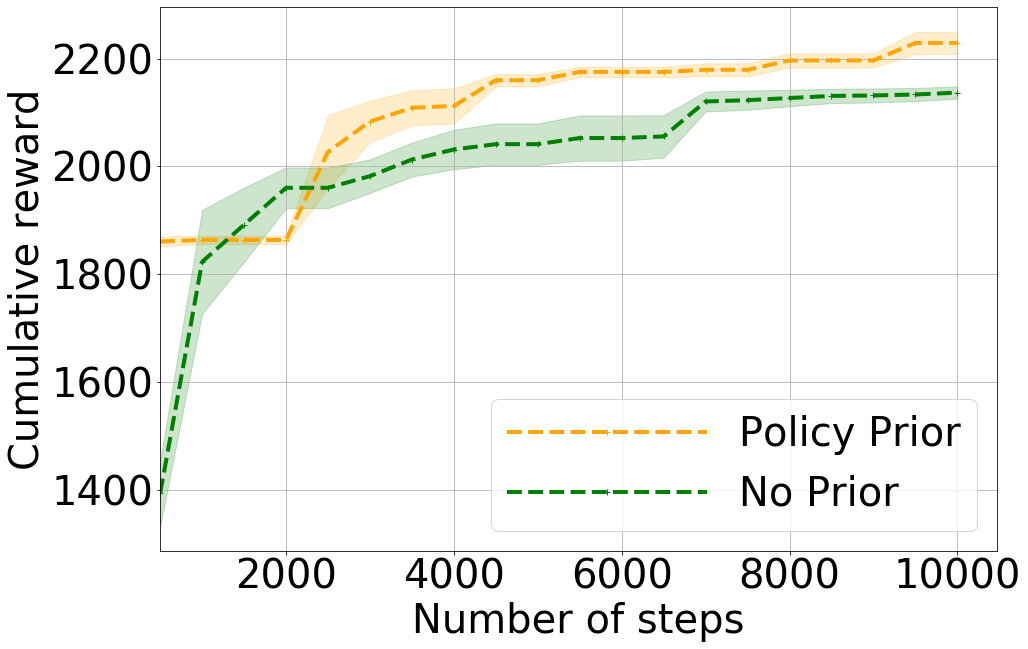
(a) Hopper-2Dim

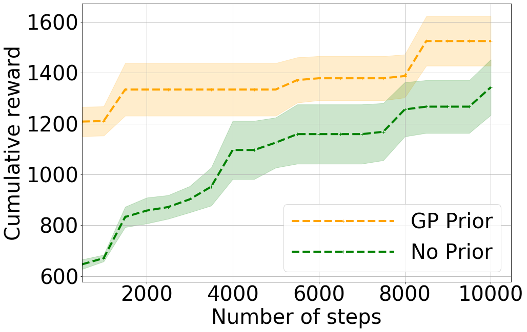
(b) Walker2D-5Dim

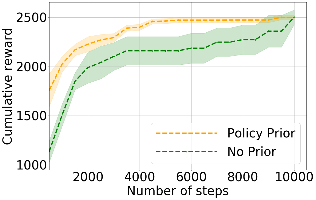
(c) Half-Cheetah-5Dim

Figure 3: Performance (cumulative reward) using a BO policy search with Policy prior on three MuJoCo tasks a) when there are two (friction and mass), and c, d) five (friction, restitution and mass of 3 body parts) unknown latent parameters of Hopper, Walker2D and Half-Cheetah. For all tasks a 500 step horizon is used.

Fig. 4 and Table Ia illustrate the sample efficiency of the policy prior introduced in Section II-B when integrated with BO policy search, evaluated on the three MuJoCo environments. For each environment we consider two settings with two (2 Dim) and five (5 Dim) unknown physics latent factors are present in the real-world, which demonstrate the efficacy of our method in both low and moderately high dimensional latent factor space.

When building the priors for these environments, in the 2 Dim setting we uniformly sample $100$ latent factors while in 5 Dim setting $250$ samples are used. We then evaluate the performance of UPN policies fetched at each sampled latent value on $10$ and $250$ different simulated environments (i.e., environments with different true latent values) for 2 Dim and 5 Dim settings, respectively. For both Bowling and Basketball tasks, we follow the same procedure to build priors for the contextual bandit agent, using $100$ latent factor combinations drawn by discretizing the latent space uniformly.

Evaluation using low cost fidelities

	MAML	DR	No Prior	Policy Prior
Walker2D - 2 Dim	514.70 $\pm$ 1.41	1530.18 $\pm$ 23.56	1353.82 $\pm$ 6.32	1602.9 $\pm$ 6.54
Walker2D - 5 Dim	552.24 $\pm$ 15.30	941.88 $\pm$ 18.17	1146.98 $\pm$ 6.00	1186.76 $\pm$ 6.53
Half-Cheetah - 2 Dim	592.76 $\pm$ 39.81	4581.58 $\pm$ 22.38	3986.11 $\pm$ 9.39	4050.92 $\pm$ 6.07
Half-Cheetah - 5 Dim	375.54 $\pm$ 3.85	1784.36 $\pm$ 9.33	2261.26 $\pm$ 11.1	2310.88 $\pm$ 7.80
Hopper - 2 Dim	394.01 $\pm$ 1.23	1603.51 $\pm$ 10.32	1930.11 $\pm$ 6.32	1928.74 $\pm$ 5.46
Hopper - 5 Dim	658.21 $\pm$ 3.69	1322.75 $\pm$ 5.90	1519.73 $\pm$ 5.06	1541.45 $\pm$ 3.96

(a) Jump start performance (cumulative episodic reward) with Policy prior on three MuJoCo tasks when there are two (2 Dim) and five (5 Dim) unknown latent parameters. For all tasks a 500 step horizon is used and jump start is averaged over 100 random episodes.

	DR	Estimated	No Prior	Policy Prior
Bowling	0.8953$\pm$ 0.0067	0.8956$\pm$ 0.0108	0.8985$\pm$ 0.0040	0.9202$\pm$ 0.0053
Basketball	0.7390 $\pm$ 0.0723	0.3145 $\pm$ 0.1147	0.8784 $\pm$ 0.0827	0.9519 $\pm$ 0.011

(b) Jump start performance (AUCCESS score) of bandit tasks. Policy search process has been conducted using low fidelity actions, 20 for Bowling and 5 for basketball.

Table I: Policy Prior’s initial transfer policy performance (jump start) on MuJoCo and Bandit tasks compared with baselines. Bold represents the best performance.

One of the key issues with UPN based online system identification is the evaluation cost during the policy search process. For instance, if we follow the PHYRE formulation for Bowling task which evaluates 100 actions per task, it would cost 40,000 interactions with the real-world to evaluate 20 BO iterations using a validation set of 20 tasks (100 actions $\times$ 20 tasks $\times$ 20 iterations). To improve the sample efficiency of this policy search process, we examine using a low fidelity evaluation by choosing the best 20 actions based on their associated rewards obtained from rollouts carried out in simulation. Following the policy search with the policy prior, we evaluate the performance of the latent conditioned policy using 100 best ranked actions on the test set (Table. Ib). Similar evaluations are carried out for the Basketball task using 5 best actions for policy search and jump start evaluated using the best 100 actions.

We designed the Basketball task such that coefficient of restitution (CoR) of objects are more impactful for the task’s goal than friction. For example, when the CoR of the ball is approximately less than 0.3, the task cannot be achieved irrespective of the friction value. We found that the Gaussianity checking step of the Policy prior (Sec. II-B1) is particularly useful to address such non-Gaussian settings (refer appendix for further details).

From the results in Fig. 3 and Table I, it is clear that considering the superior sample efficiency offered through policy search, combined with the consistently good jump start performances, the prior policy is a beneficial tool for efficient learning in the parameterisable environments considered in this work. For low dimensional cases (e.g. 2 Dim), DR performs on par or better than BO methods, likely due to the low randomness offered by the environment. However, when the number of unknown parameters increases, DR performs poorer than policy search methods.

IV Related Work

As a solution to sample inefficiency in many deep RL applications, efficient simulation based transfer (i.e., Sim2Real) has become a necessary, albeit a challenging task. The fundamental requirement for such transfer is that simulation and real-world having some shared basis for transfer, which has been studied in different granularities. One such simulation-in-the-loop approach, as shown by [3, 4, 25, 26, 27, 28, 29, 30, 31], is system identification, which adapts the simulator to closely match the real-world trajectories (i.e., ‘grounding’,) by minimising the trajectory difference (i.e., residual) between the model and real-world. As an optimisation workflow, they iteratively execute a simulator trained policy in the real-world and improve simulated latent factor estimates. However, these attempts suffer from several key issues: a) residual minimisation is unaware of goal-conditioned latent factors, which may overexert the model learning process; b) designing a residual measure that guarantees to converge to the true latent estimate is challenging as shown by [26], who used a weighted importance measure for this purpose; c) iterative policy training in simulator and real-world is not practical for time-sensitive tasks; and d) latent estimation being sensitive to the initialisation, can lead to suboptimal estimations.

To address some of the issues with system identification, task conditioned policy learning methods have been proposed. One such approach is domain randomisation (DR), which trains agents in a range of randomised latent factors to find invariant task policies through different dynamics [8, 9, 32] . While it is relatively simple to implement, this method has shown to produce overly robust and conservative policies that may not be capable of quickly adapting to a given environment [10]. Moreover, [32] observed that over randomisation can have an detrimental effect on DR learning, which raises the difficulty of identifying the boundaries of DR training.

Instead of learning conservative policies, a line of research has studied evaluating policies directly in the real-world task (i.e., direct policy search) to improve the simulated model [33]. However, this introduced the difficulty of iteratively training simulated policies and a likely high evaluation cost in the real-world. In a novel approach, [17] introduced Universal Policy networks (UPN), an RL agent model trained to learn a large set of policies, each of which is conditioned on a latent factor. They showed this model was capable of generalising to estimate policies for unseen latent values. To estimate latent factors from observations, they used a DL based system identification model, but [11, 18] successfully demonstrated using direct policy search with UPN by estimating latent factors from an evaluated real-world policy such that the policy emitted from UPN for estimated latent values will improve the policy transfer. To estimate the latent values, they used Bayesian Optimisation (BO)[13] with Gaussian Processes (GP) [34] as a cheap surrogate function of the true function. Our approach, while using a similar workflow, improves the sample efficiency of policy search process over these methods by instilling prior information about the policy and dynamic function behaviours.

Meta learning is another line of research that addresses fast adaptation to a new task. Model Agnostic meta-learning (MAML)[23] introduces a gradient based parameters optimisation method for a set of tasks such that adapting to a new task is sample efficient. Nagabandi et al.[35] extends this concept to learn a model prior capable of rapidly adapting to a new task, whereas, Mendonca et al. [36] and Yu et al.[37] meta trains a context variable that can be used as a latent factor to condition a trained UPN. We use MAML as one of our baselines to examine the sample efficiency of meta-learning when adapting to a new environment.

V Conclusion

In this work, we proposed a novel model-based prior to improve the sample efficiency of direct policy search when learning in an unknown environment. Using a numerical simulator to evaluate universal policy network (UPN) based policies in varied simulated environments, our proposed approach was used to obtain an estimate of its inter-policy similarity. This was then integrated with a Gaussian Process based Bayesian Optimisation workflow in order to efficiently identify appropriate policies from the UPN. We empirically evaluated our method in five MuJoCo and bandit learning environments, and demonstrated its superior sample efficiency in terms of search convergence and transfer jump start performances compared to competing baselines.

VI Appendix

VI-A Policy Prior Integrated Policy Search Performances - Extended

Fig. 4 shows the performance of Policy prior integrated Bayesian Optimisation policy search, in terms of the cumulative reward, on three MuJoCo tasks, Hopper, Walker2D and Half-Cheetah. Fig. 5 shows the Policy prior’s policy search performance on two bandit tasks, Bowling and Basketball, in terms of AUCCESS score [16, Sec. 3.2].

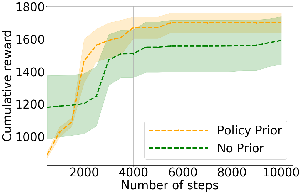
(a) 2Dim-Walker2D

(b) 5Dim-Walker2D

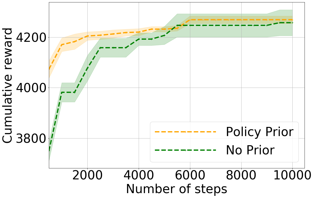
(c) 2Dim-Half-Cheetah

(d) 5Dim-Half-Cheetah

(e) 2Dim-Hopper

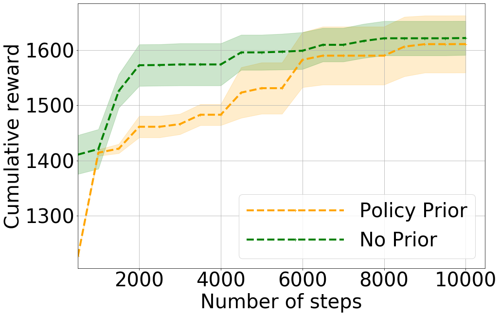
(f) 5Dim-Hopper

Figure 4: Performance in terms of the cumulative reward using a Bayesian Optimisation policy search with Policy prior on three MuJoCo tasks, a,c,e) when there are two unknown latent parameters, mass and friction in the real world, and b,d,f) when there are five unknown latent parameters: friction, restitution and mass of 3 body parts Hopper, Walker2D and Half-Cheetah. For all tasks a 500 step horizon is used.

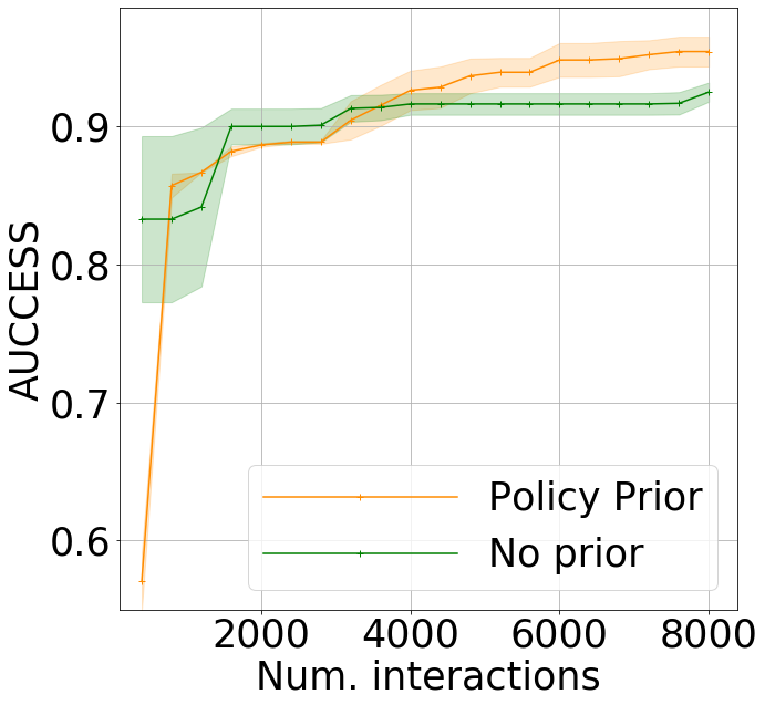
(a) Bowling

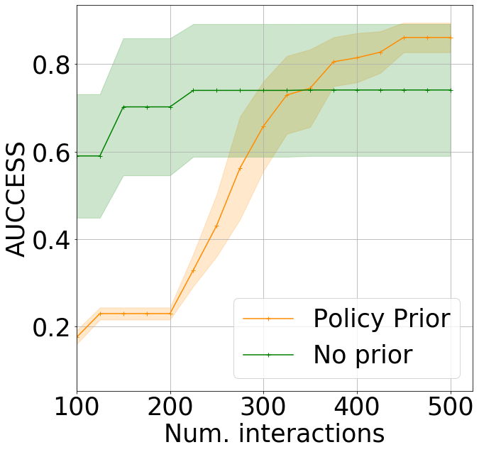
(b) Basketball

Figure 5: Policy Prior’s policy search performances in terms of the AUCCESS score, on the validation task set. Policy search has been conducted using a low fidelity action set for bandit tasks, (a) Bowling task with 20 best actions and (b) Basketball task with 5 best actions.

VI-B Ablation Study: Checking for Gaussianity of Prior in Basketball Task

Basketball task is designed such that CoR of objects are more impactful for the task’s goal than friction. This is elucidated in Fig. 6a and 6b, which show the mean and variance of jump start performances of basketball UPN policies, when conditioned at 10$\times$10 grid of latent values and then transferred to 9 different ground truth settings. In essence, when the CoR of the ball is approximately less than 0.3, the task can not be achieved irrespective of the friction value. We utilise this skewed setting to investigate the behaviour of our Policy prior in tasks that do not respond equally to all latent factors involved.

Fig. 6c shows that during BO policy search, Policy Prior without the Gaussianity check performing worse than the no prior baseline on the Basketball task. We posit this is due to the non-Gaussian distribution of the Policy Prior and to remedy this issue, we filter out non-Gaussian observations with p-value less than 0.1 using Kolmogorov-Smirnov Goodness-of-Fit Test. In the best 5 action setting of the basketball task we are using, it filters out 59 observations out of 100. With this modified prior, we run the trial again and Fig. 5b shows the improved BO policy search performance. This relatively simple step can assist in making the Policy Prior useful for tasks irrespective of their latent factor distribution. However, it comes with a caveat that the loss of observations could reduce the effect of the prior if most of the observations are filtered out.

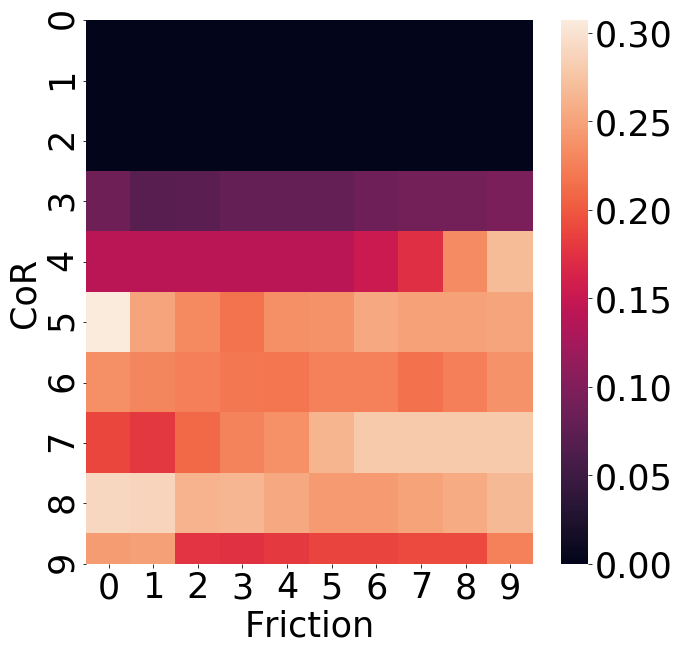
(a)

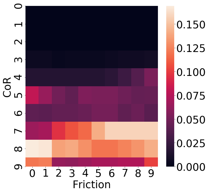
(b)

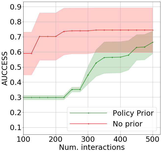
(c)

Figure 6: Basketball task’s non-Gaussian latent factor distribution’s effect on BO. a) Mean and b) variance of jump start performances of basketball UPN policies when conditioned at 10$\times$10 grid of latent values and evaluated across 9 different ground truth settings (combinations of friction and CoR at 0.2, 0.5, 0.8). c) Policy prior’s BO convergence performance in Basketball task without the Gaussianity check, using only the 5 best actions at each evaluation. All evaluations are executed in the simulated environment with Basketball validation test set.

VI-C DQN Based Universal Policy Network

For training UPNs for contextual bandit tasks, we use Deep Q-Networks [2] as the underlying agent. When implementing the DQN based UPN, we augment a DQN architecture adopted from PHYRE [16] by supporting conditioning with latent factors in addition to actions (Fig. 7). For this purpose we use a FiLM layer [38] due to its ability to modulate between two signals. We train this model on simulator generated trajectories by sampling latent factors for a given task.

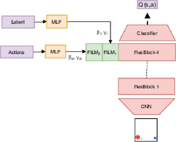
Figure 7: A DQN based UPN design. Latent and action vectors are encoded using MLP layers, which are used to condition the observations encoded by a residual network [39] using FiLM layer [38]. $\beta$ and $\gamma$ are parameters learnt by FiLM to modulate conditioning.

VI-D Universal Policy Network Training

We use the DQN based UPN implementation introduced in Sec. VI-C to find policies for our contextual bandit tasks. In these tasks, we keep the density of objects consistent and maintain friction and coefficient of restitution (CoR) as the unknown latent factors. When training the UPN, we select 12 combinations of friction and CoR in the range of [0, 1] from a grid with resolution of 0.3 as conditioning latent points. We then train the UPN on tasks in the training fold of dataset, each of which is replicated on all 12 latent factor combinations (i.e., each task is simulated under all sampled latent factor settings). In order to decide when the UPN has sufficiently converged to an overall good policy, we evaluate the UPN’s policy at 100 sampled latent value points, which are then transferred to 9 different simulated ground truth latent values as shown in Fig. 8. A sufficiently converged UPN policy should give relatively high rewards when the ground truth latent values approximately overlap with the sampled latent values in the UPN. Leveraging this strategy, we selected UPN models trained for 32 batches of 24,000 and 48,000 updates for Bowling and Basketball tasks respectively. Furthermore, this verification establishes that our DQN based UPN can learn latent conditioned policies successfully.

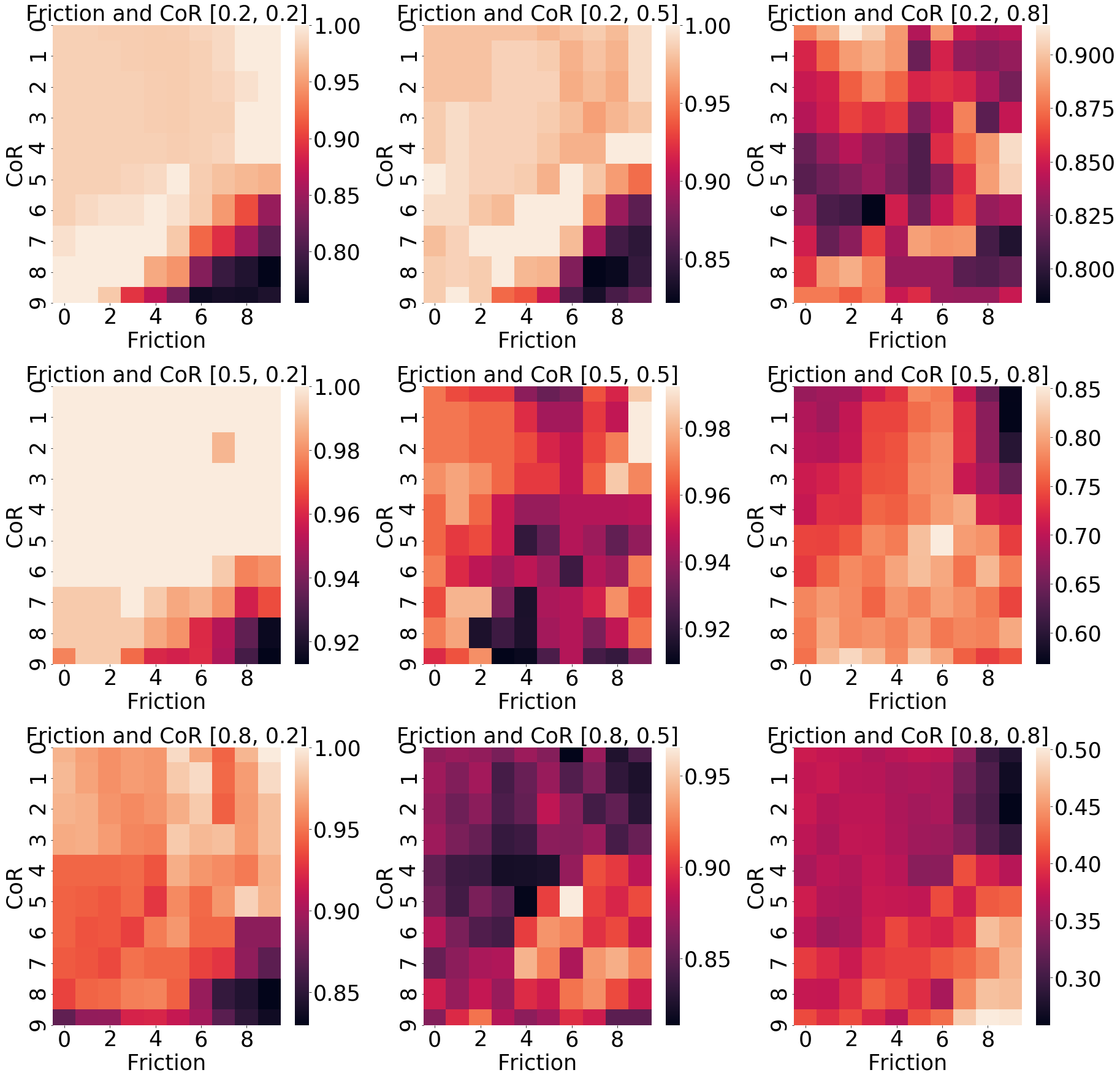
Figure 8: A simple strategy to decide whether the UPN has converged. 100 sampled latent value combinations of friction and CoR are evaluated on the UPN to select a policy and then transferred to 9 different environment settings. The title of each subplot refers to the ground truth friction and CoR value of the environment in which the policy is being evaluated at. A well trained UPN should provide policies that yield high rewards when UPN latent values and ground truth values match.

VI-E UPN Training performances

Fig. 9 shows the training performances of Universal Policy Networks (UPN) on three MuJoCo environments, each under two settings of two (2D) and five (5D) unknown latent factors. In the 2D setting, mass of a body node and friction of the tasks are unknown, whereas in the 5D setting, friction, restitution and mass of 3 body parts are unknown.

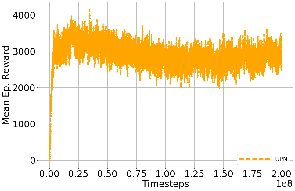
(a) Hopper-2D

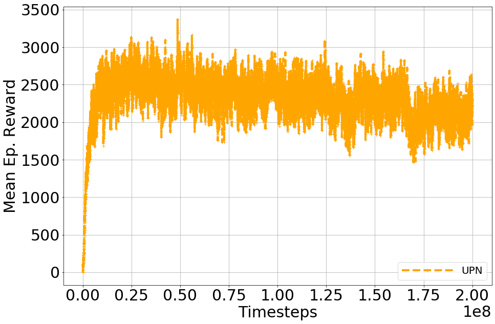
(b) Hopper-5D

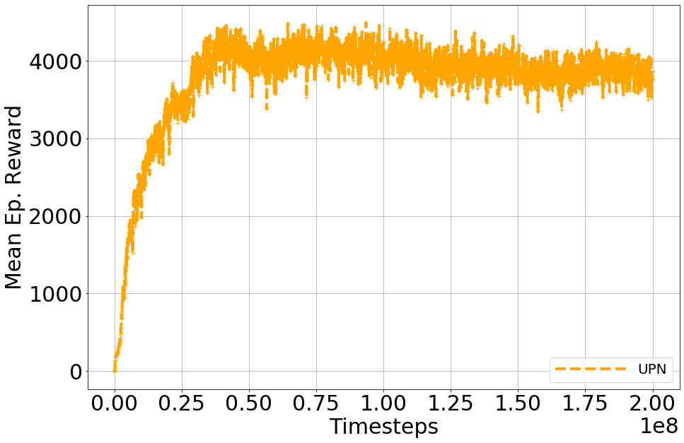
(c) Walker-2D

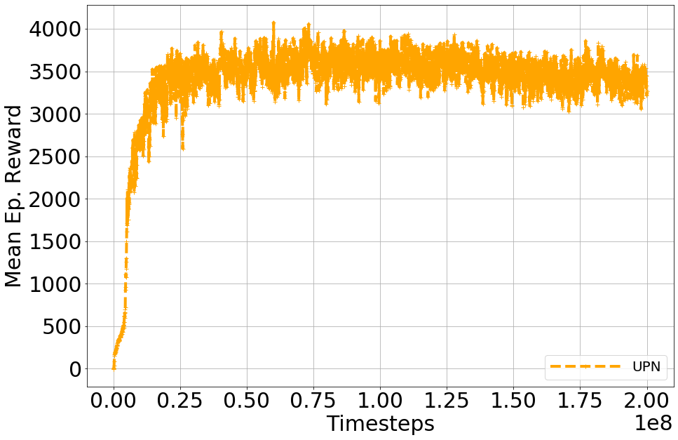
(d) Walker-5D

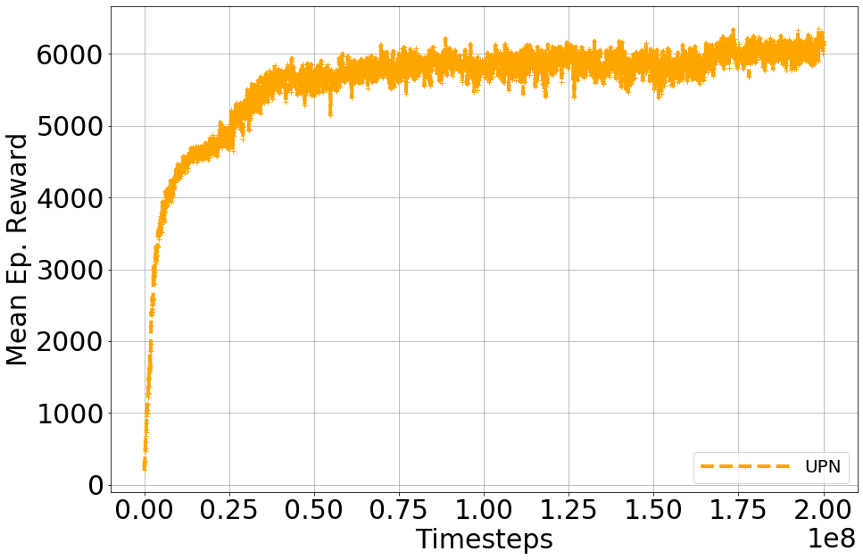
(e) Half-Cheetah-2D

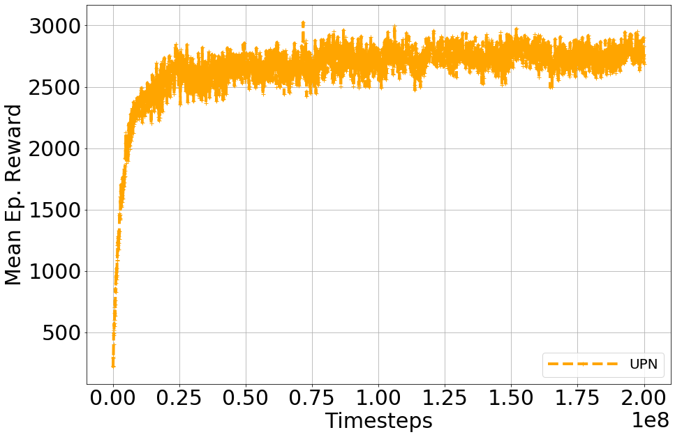
(f) Half-Cheetah-5D

Figure 9: UPN average episodic reward during training (in simulation) for three MuJoCo tasks: Hopper, Walker2D and Half-Cheetah. a, c, e) 2 unknown latent factors (2D) setting (mass and friction), and b, d, f) 5 unknown latent factors (5D) setting (friction, restitution and mass of 3 body parts).

VI-F Implementation Details

When conducting BO based policy search, we used GPy[40] to build the GP model and Emukit [41] for Bayesian Optimisation execution. All Policy Prior and No Prior results reported are averaged over 5 trials, each of which is initialised with its random number generator seed mutually exclusively set to one of 50, 100, 150, 500 and 1000. For all BO operations, we use RBF kernel, Expected improvement (EI) as the acquisition function, with LBFGS as the optimiser. During BO, to maintain the matrix is well-conditioned, we verify the condition number of the kernel matrix is at most 25,000 and add random noise from a range of [0.1, $10^{-5}$] to the diagonal if it exceeds this threshold.

For no prior baseline, the process starts with 3 random samples and proceeds to build the GP. In MuJoCo tasks, BO samples within the bounds [0, 1], as all features are normalised. For bandit tasks, friction range is [0, 3] while CoR is [0, 1].

For MuJoCo tasks, depending on the setting (2D or 5D), we set the ground truth to a vector of length 2 or 5, generated with NumPy random.uniform() with random number generator seed set to 1. To separate the real-world from the simulated environment, we use a damping value of 3 using PyDart simulator’s set_damping_coefficient API call.

Contextual bandit tasks maintain standard three folds of task sets and a maximum action size to sample from. The Bowling task uses 5000 actions, with 100 tasks in total split to 60 training, 20 validation and 20 test tasks. The Basketball task utilises 40,000 actions, with a dataset containing 25 tasks, split into 15 training, 5 validation and 5 test sets. When setting up the real-world, for both tasks a damping of 0.8 is used whereas in the simulated environment no damping value is used. For the Estimated baseline, 6,000 real-world interactions for the Bowling task and 1,500 for the Basketball task have been used to minimise the difference between real-world and simulated trajectories.

References

- [1] D. Silver, A. Huang, C. J. Maddison, A. Guez, L. Sifre, G. Van Den Driessche, J. Schrittwieser, I. Antonoglou, V. Panneershelvam, M. Lanctot et al., “Mastering the game of go with deep neural networks and tree search,” nature, vol. 529, no. 7587, pp. 484–489, 2016.
- [2] V. Mnih, K. Kavukcuoglu, D. Silver, A. A. Rusu, J. Veness, M. G. Bellemare, A. Graves, M. Riedmiller, A. K. Fidjeland, G. Ostrovski et al., “Human-level control through deep reinforcement learning,” nature, vol. 518, no. 7540, pp. 529–533, 2015.
- [3] P. Abbeel, M. Quigley, and A. Y. Ng, “Using inaccurate models in reinforcement learning,” in Proceedings of the 23rd International Conference on Machine Learning, ser. ICML ’06. New York, NY, USA: Association for Computing Machinery, 2006, pp. 1–8. [Online]. Available: https://doi.org/10.1145/1143844.1143845
- [4] A. Farchy, S. Barrett, P. MacAlpine, and P. Stone, “Humanoid robots learning to walk faster: From the real world to simulation and back,” in AAMAS, 2013, pp. 39–46.
- [5] D. Zheng, V. Luo, J. Wu, and J. B. Tenenbaum, “Unsupervised learning of latent physical properties using Perception-Prediction networks,” in Proceedings of the Thirty-Fourth UAI 2018, Monterey, California, USA, August 6-10, 2018, A. Globerson and R. Silva, Eds. AUAI Press, 2018, pp. 497–507.
- [6] M. B. Chang, T. Ullman, A. Torralba, and J. B. Tenenbaum, “A compositional Object-Based approach to learning physical dynamics,” Dec. 2016.
- [7] Z. Xu, J. Wu, A. Zeng, J. B. Tenenbaum, and S. Song, “Densephysnet: Learning dense physical object representations via multi-step dynamic interactions,” in Robotics: Science and Systems XV, University of Freiburg, Freiburg im Breisgau, Germany, June 22-26, 2019, A. Bicchi, H. Kress-Gazit, and S. Hutchinson, Eds., 2019. [Online]. Available: https://doi.org/10.15607/RSS.2019.XV.046
- [8] J. Tobin, R. Fong, A. Ray, J. Schneider, W. Zaremba, and P. Abbeel, “Domain randomization for transferring deep neural networks from simulation to the real world,” in 2017 IEEE/RSJ International Conference on Intelligent Robots and Systems (IROS), 2017, pp. 23–30.
- [9] F. Sadeghi and S. Levine, “CAD2RL: real single-image flight without a single real image,” in Robotics: Science and Systems XIII, MIT, USA, 2017, N. M. Amato, S. S. Srinivasa, N. Ayanian, and S. Kuindersma, Eds., 2017.
- [10] M. Sheckells, G. Garimella, S. Mishra, and M. Kobilarov, “Using data-driven domain randomization to transfer robust control policies to mobile robots,” in 2019 International Conference on Robotics and Automation (ICRA), 2019, pp. 3224–3230.
- [11] W. Yu, V. C. Kumar, G. Turk, and C. K. Liu, “Sim-to-real transfer for biped locomotion,” in Proc. of The International Conference on Intelligent Robots and Systems (IROS), 2019.
- [12] A. Lazaric, “Transfer in reinforcement learning: a framework and a survey,” in Reinforcement Learning. Springer, 2012, pp. 143–173.
- [13] P. I. Frazier, “A tutorial on bayesian optimization,” arXiv preprint arXiv:1807.02811, 2018.
- [14] T. T. Joy, S. Rana, S. Gupta, and S. Venkatesh, “A flexible transfer learning framework for bayesian optimization with convergence guarantee,” Expert Systems with Applications, vol. 115, pp. 656–672, 2019.
- [15] G. Brockman, V. Cheung, L. Pettersson, J. Schneider, J. Schulman, J. Tang, and W. Zaremba, “Openai gym,” CoRR, vol. abs/1606.01540, 2016. [Online]. Available: http://arxiv.org/abs/1606.01540
- [16] A. Bakhtin, L. van der Maaten, J. Johnson, L. Gustafson, and R. Girshick, “PHYRE: A new benchmark for physical reasoning,” in NeurIPS, 2019, pp. 5082–5093.
- [17] W. Yu, J. Tan, C. K. Liu, and G. Turk, “Preparing for the unknown: Learning a universal policy with online system identification,” in Robotics: Science and Systems XIII, Massachusetts Institute of Technology, Cambridge, Massachusetts, USA, July 12-16, 2017, N. M. Amato, S. S. Srinivasa, N. Ayanian, and S. Kuindersma, Eds., 2017. [Online]. Available: http://www.roboticsproceedings.org/rss13/p48.html
- [18] W. Yu, C. K. Liu, and G. Turk, “Policy transfer with strategy optimization,” in International Conference on Learning Representations, 2019. [Online]. Available: https://openreview.net/forum?id=H1g6osRcFQ
- [19] T. S. community. (2008) scipy.stats.kstest. [Online]. Available: https://docs.scipy.org/doc/scipy/reference/generated/scipy.stats.kstest.html
- [20] N. Heckert and J. Filliben, “Nist/sematech e-handbook of statistical methods; chapter 1: Exploratory data analysis,” 2003-06-01 2003.
- [21] E. Todorov, T. Erez, and Y. Tassa, “Mujoco: A physics engine for model-based control,” in 2012 IEEE/RSJ International Conference on Intelligent Robots and Systems. IEEE, 2012, pp. 5026–5033.
- [22] V. Blomqvist, “Pymunk simulator,” http://www.pymunk.org/.
- [23] C. Finn, P. Abbeel, and S. Levine, “Model-agnostic meta-learning for fast adaptation of deep networks,” in International Conference on Machine Learning. PMLR, 2017, pp. 1126–1135.
- [24] J. Schulman, F. Wolski, P. Dhariwal, A. Radford, and O. Klimov, “Proximal policy optimization algorithms,” CoRR, vol. abs/1707.06347, 2017. [Online]. Available: http://arxiv.org/abs/1707.06347
- [25] S. Zhu, A. Kimmel, K. E. Bekris, and A. Boularias, “Fast model identification via physics engines for data-efficient policy search,” in Proceedings of the 27th International Joint Conference on Artificial Intelligence, ser. IJCAI’18. AAAI Press, 2018, pp. 3249–3256.
- [26] Y. Chebotar, A. Handa, V. Makoviychuk, M. Macklin, J. Issac, N. D. Ratliff, and D. Fox, “Closing the sim-to-real loop: Adapting simulation randomization with real world experience,” in International Conference on Robotics and Automation, ICRA 2019, Montreal, QC, Canada, May 20-24, 2019. IEEE, 2019, pp. 8973–8979. [Online]. Available: https://doi.org/10.1109/ICRA.2019.8793789
- [27] Y. Du, O. Watkins, T. Darrell, P. Abbeel, and D. Pathak, “Auto-tuned sim-to-real transfer,” arXiv preprint arXiv:2104.07662, 2021.
- [28] A. Allevato, E. S. Short, M. Pryor, and A. Thomaz, “Tunenet: One-shot residual tuning for system identification and sim-to-real robot task transfer,” in Conference on Robot Learning. PMLR, 2020, pp. 445–455.
- [29] A. D. Allevato, E. Schaertl Short, M. Pryor, and A. L. Thomaz, “Iterative residual tuning for system identification and sim-to-real robot learning,” Autonomous Robots, vol. 44, no. 7, pp. 1167–1182, 2020. [Online]. Available: https://doi.org/10.1007/s10514-020-09925-w
- [30] J. P. Hanna and P. Stone, “Grounded action transformation for robot learning in simulation,” in AAAI. AAAI Press, 2017, pp. 4931–4932.
- [31] S. Desai, H. Karnan, J. P. Hanna, G. Warnell, and a. P. Stone, “Stochastic grounded action transformation for robot learning in simulation,” in 2020 IEEE/RSJ International Conference on Intelligent Robots and Systems (IROS), 2020, pp. 6106–6111.
- [32] J. Matas, S. James, and A. J. Davison, “Sim-to-real reinforcement learning for deformable object manipulation,” in Conference on Robot Learning. PMLR, 2018, pp. 734–743.
- [33] V. Heidrich-Meisner and C. Igel, “Hoeffding and bernstein races for selecting policies in evolutionary direct policy search,” in Proceedings of the 26th Annual International Conference on Machine Learning, ser. ICML ’09. New York, NY, USA: Association for Computing Machinery, 2009, pp. 401–408. [Online]. Available: https://doi.org/10.1145/1553374.1553426
- [34] C. E. Rasmussen, “Gaussian processes in machine learning,” pp. 63–71, 2004.
- [35] A. Nagabandi, I. Clavera, S. Liu, R. S. Fearing, P. Abbeel, S. Levine, and C. Finn, “Learning to adapt in dynamic, real-world environments through meta-reinforcement learning,” in International Conference on Learning Representations, 2018.
- [36] R. Mendonca, X. Geng, C. Finn, and S. Levine, “Meta-reinforcement learning robust to distributional shift via model identification and experience relabeling,” arXiv preprint arXiv:2006.07178, 2020.
- [37] W. Yu, J. Tan, Y. Bai, E. Coumans, and S. Ha, “Learning fast adaptation with meta strategy optimization,” IEEE Robotics and Automation Letters, vol. 5, no. 2, pp. 2950–2957, 2020.
- [38] E. Perez, F. Strub, H. De Vries, V. Dumoulin, and A. Courville, “Film: Visual reasoning with a general conditioning layer,” in Proceedings of the AAAI Conference on Artificial Intelligence, vol. 32, no. 1, 2018.
- [39] K. He, X. Zhang, S. Ren, and J. Sun, “Deep residual learning for image recognition,” in Proceedings of the IEEE conference on computer vision and pattern recognition, 2016, pp. 770–778.
- [40] GPy, “GPy: A gaussian process framework in python,” http://github.com/SheffieldML/GPy, since 2012.
- [41] A. Paleyes, M. Pullin, M. Mahsereci, N. Lawrence, and J. González, “Emulation of physical processes with emukit,” in Second Workshop on Machine Learning and the Physical Sciences, NeurIPS, 2019.