Entropic Fictitious Play
for Mean Field Optimization Problem

Abstract

We study two-layer neural networks in the mean field limit, where the number of neurons tends to infinity. In this regime, the optimization over the neuron parameters becomes the optimization over the probability measures, and by adding an entropic regularizer, the minimizer of the problem is identified as a fixed point. We propose a novel training algorithm named entropic fictitious play, inspired by the classical fictitious play in game theory for learning Nash equilibriums, to recover this fixed point, and the algorithm exhibits a two-loop iteration structure. Exponential convergence is proved in this paper and we also verify our theoretical results by simple numerical examples.

Keywords: mean field optimization, neural network, fictitious play, relative entropy, free energy function

1 Introduction

Deep learning has achieved unprecedented success in numerous practical scenarios, including computer vision, natural language processing and even autonomous driving, which leverages deep reinforcement learning techniques (Krizhevsky et al., 2012; Goldberg, 2016; Arulkumaran et al., 2017). Stochastic gradient algorithms (SGD) and their variants have been widely used to train neural networks, that is, to minimize networks’ loss and thereby to fit the data available effectively (Le Cun et al., 1998; Kingma and Ba, 2014). However, due to the complicated network structures and the non-convexity of typical optimization objectives, mathematical guarantees of convergence to the optimizer remain elusive. Recent studies on the insensibility of the number of neurons on one layer when it is sufficiently large (Hastie et al., 2022), and the feasibility of interchanging the neurons on one layer (Nguyen and Pham, 2020; Rotskoff and Vanden-Eijnden, 2018) both motivated the investigation of mean field regime. In practice, over-parameterized neural networks with a large number of neurons are commonly employed in order to achieve high performance (Huang et al., 2017). This further motivates researchers to view neurons as random variables following a probability distribution and the summation over neurons as an expectation with respect to this distribution (Sirignano and Spiliopoulos, 2020).

Another appealing approach to address the global convergence of over-parameterized networks is through the neural tangent kernel (NTK) regime (Jacot et al., 2018). In this regime, it is believed that when the network width tends to infinity, the parameter updates, driven by stochastic gradient descent, do not significantly deviate from i.i.d Gaussian initialization, and these updates are called lazy training (Tzen and Raginsky, 2020; Chizat et al., 2019). As a result, training of neural networks can be depicted as regression with a fixed kernel given by linearization at initialization, leading to the exponential convergence (Jacot et al., 2018). By appropriate time rescaling, it is possible for the dynamics of the kernel method to track the SGD dynamics closely (Mei et al., 2019; Allen-Zhu et al., 2019). Other studies, such as Dou and Liang (2021), explore the reproducing kernel Hilbert space and demonstrate that the gradient flow indeed converges to the kernel ridgeless regression with an adaptive kernel. Besides in Chen et al. (2020), the researchers extend the definition of the kernel and show that the training with an appropriate regularizer also exhibits behaviors similar to the kernel method. However, the kernel behavior primarily manifests during the early stages of the training process, whereas the mean field model reveals and explains the longer-term characteristics (Mei et al., 2019). Furthermore, another advantage of the mean field settings compared to NTK is the presence of feature learning, in contrast to the perspective of random feature (Suzuki, 2019; Ghorbani et al., 2019).

In the mean field limit where neurons become infinitely many, the dynamics of the neuron parameters under gradient descent can be understood as a gradient flow of measures in Wasserstein-$2$ space, providing a geometric interpretation of the learning algorithm. This flow is also described by a PDE system where the unknown is the density function of the measure. Well-posedness of the PDE system, discretization errors and finite-time propagation of chaos are studied in recent works (Nguyen and Pham, 2020; Mei et al., 2019; Fang et al., 2021; Araújo et al., 2019; Sirignano and Spiliopoulos, 2022). On the other hand, extensive analysis has been conducted to investigate the convergence of such dynamics to their equilibrium. The convergence of gradient flows modeling shallow networks is studied in Chizat and Bach (2018); Mei et al. (2019); Hu et al. (2021); more recent works extend the gradient-flow formulation and study deep network structures (Fang et al., 2021; Nguyen and Pham, 2020). Sufficient conditions for the convergence under non-convex loss functions have been given in Nguyen and Pham (2020), and the discriminatory properties of the non-linear activation function have been exploited in Sirignano and Spiliopoulos (2022); Rotskoff and Vanden-Eijnden (2018) to deduce the convergence.

In this paper, one key assumption is the convexity of the objective functional with respect to its measure-valued argument. This assumption has been exploited by many recent works. Notably, Nitanda et al. (2022) have established the exponential convergence of the entropy-regularized problem in both discrete and continuous-time settings by utilizing the log-Sobolev inequality (LSI), following the observations in Nitanda et al. (2021). Additionally, Nitanda and Suzuki (2017) estimate the generalization error and prove a polynomial convergence rate by leveraging quadratic expansions of the loss function. Wei et al. (2019) also prove polynomial convergence rates in different scenarios, where they add noise to the gradient descent and assume the activation and regularization functions are homogeneous.

With the existing convergence results on gradient flows for the mean field optimization problem in mind, the following question arises to us:

Do there exist dynamics other than gradient flows
that solve the (regularized) mean field optimization efficiently?

We believe the quest for its answer will not be wasted efforts, as it may lead to potentially highly performant algorithms for training neural networks, and also because the dynamics similar to that we consider in this paper have already found applications to various mean field problems.

We recall the classical fictitious play in game theory originally introduced by Brown Brown (1951) to learn Nash equilibriums. During the fictitious play, in each round of repeated games, each player optimally responds to the empirical frequency of actions taken by their opponents (hence the name). While the fictitious play does not necessarily converge in general cases (Shapley, 1964), it does converge for zero-sum games (Robinson, 1951) and potential games (Monderer and Shapley, 1996). More recently, this method has been revisited in the context of mean field games (Cardaliaguet and Hadikhanloo, 2017; Hadikhanloo and Silva, 2019; Perrin et al., 2020; Lavigne and Pfeiffer, 2022).

In this paper, we draw inspiration from the classical fictitious play and propose a similar algorithm, called entropic fictitious play (EFP), to solve mean field optimization problems emerging from the training of two-layer neural networks. Our algorithm shares a two-loop iteration structure with the particle dual average (PDA) algorithm, recently proposed by Nitanda et al. (2021). They estimated the computational complexity and conducted various numerical experiments for PDA to show its effectiveness in solving regularized mean field problems. However, PDA is essentially different from our EFP algorithm and their differences will be discussed in Sections 2 and 4.

2 Problem Setting

Let us first recall how the (convex) mean field optimization problem emerges from the training of two-layer neural networks. While the universal representation theorem tells us that a two-layer network can arbitrarily well approximate the continuous function on the compact time interval (Cybenko, 1989; Barron, 1993), it does not tell us how to find the optimal parameters. One is faced with the non-convex optimization problem

$$\min_{\beta_{n,i}\in\mathbb{R},\alpha_{n,i}\in\mathbb{R}^{d},\gamma_{n,i}\in\mathbb{R}}\int_{\mathbb{R}\times\mathbb{R}^{d}}\ell\biggl{(}y,\frac{1}{n}\sum_{i=1}^{n}\beta_{n,i}\varphi(\alpha_{n,i}\cdot z+\gamma_{n,i})\biggr{)}\,\nu(dy\,dz),$$ (1)

where $\theta\mapsto\ell(y,\theta)$ is convex for every $y$, $\varphi:\mathbb{R}\rightarrow\mathbb{R}$ is a bounded, continuous and non-constant activation function, and $\nu$ is a measure of compact support representing the data. Denote the empirical law of the parameters $m^{n}$ by $m^{n}=\frac{1}{n}\sum_{i=1}^{n}\delta_{(\beta_{n,i},\alpha_{n,i},\gamma_{n,i})}$. Then the neural network output can be written by

$$\frac{1}{n}\sum_{i=1}^{n}\beta_{n,i}\varphi(\alpha_{n,i}\cdot z+\gamma_{n,i})=\int_{\mathbb{R}^{d+2}}\beta\varphi(\alpha\cdot z+\gamma)\,m^{n}(d\beta\,d\alpha\,d\gamma).$$

For technical reasons we may introduce a truncation function $h(\cdot)$ whose parameter is denoted by $\beta$ as in Hu et al. (2021). To ease the notation we denote $x=(\beta,\alpha,\gamma)\in\mathbb{R}^{d+2}$ and $\hat{\varphi}(x,z)=h(\beta)\varphi(\alpha\cdot z+\gamma)$. Denote also by $\mathbb{E}^{m}=\mathbb{E}^{X\sim m}$ the expectation of the random variable $X$ of law $m$. Now we relax the original problem (1) and study the mean field optimization problem over the probability measures,

$$\min_{m\in\mathcal{P}(\mathbb{R}^{d})}F(m),\quad\text{where}~{}F(m)\coloneqq\int_{\mathbb{R}^{d}}\ell\bigr{(}y,\mathbb{E}^{m}[\hat{\varphi}(X,z)]\bigl{)}\,\nu(dy\,dz)$$ (2)

This reformulation is crucial, because the potential functional $F$ defined above is convex in the space of probability measure. In this paper, as in Hu et al. (2021); Mei et al. (2018), we shall add a relative entropy term $H(m|g)\coloneqq\int_{x\in\mathbb{R}^{d}}\log\frac{dm}{dg}(x)\,m(dx)$ in order to regularize the problem. The regularized problem then reads

$$\min_{m\in\mathcal{P}(\mathbb{R}^{d})}V^{\sigma}(m),\quad\text{where}~{}V^{\sigma}(m)\coloneqq F(m)+\frac{\sigma^{2}}{2}H(m|g).$$ (3)

Here we choose the probability measure $g$ to be a Gibbs measure with energy function $U$, that is, the density of $g$ satisfies $g(x)\propto\exp\bigl{(}-U(x)\bigr{)}$. It is worth noting that if a probability measure has finite entropy relative to the Gibbs measure $g$, then it is absolutely continuous with respect to the Lebesgue measure. Hence the density of $m$ exists whenever $V^{\sigma}(m)$ is finite. In the following, we will abuse the notation and use the same letter to denote the density function of $m$.

Since $F$ is convex, together with mild conditions, the first-order condition says that $m^{*}$ is a minimizer of $V^{\sigma}$ if and only if

$$\frac{\delta F}{\delta m}(m^{*},x)+\frac{\sigma^{2}}{2}\log m^{*}(x)+\frac{\sigma^{2}}{2}U(x)=\text{constant},$$ (4)

where $\frac{\delta F}{\delta m}$ is the linear derivative, whose definition is postponed to Assumption 1 below. Further, note that $m^{*}$ satisfying (4) must be an invariant measure to the so-called mean field Langevin (MFL) diffusion:

$$dX_{t}=-\biggl{(}\nabla_{x}\frac{\delta F}{\delta m}(m_{t},X_{t})+\frac{\sigma^{2}}{2}\nabla_{x}U(X_{t})\biggr{)}\,dt+\sigma\,dW_{t},\quad\text{where}~{}m_{t}\coloneqq\operatorname{Law}(X_{t}).$$

In Hu et al. (2021) it has been shown that the MFL marginal law $m_{t}$ converges towards $m^{*}$, and this provides an algorithm to approximate the minimizer $m^{*}$.

The starting point of our new algorithm is to view the first-order condition (4) as a fixed pointed problem. Given $m\in\mathcal{P}(\mathbb{R}^{d})$, let $\Phi(m)$ be the probability measure such that

$$\frac{\delta F}{\delta m}(m,x)+\frac{\sigma^{2}}{2}\log\Phi(m)(x)+\frac{\sigma^{2}}{2}U(x)=\text{constant}.$$ (5)

By definition, a probability measure $m$ satisfies the first-order condition (4) if and only if $m$ is a fixed point of $\Phi$. Throughout the paper we shall assume that there exists at most one probability measure satisfying the first-order condition (equivalently, there exists at most one fixed point for $\Phi$). This is true when the objective functional $F$ is convex. Indeed, as the relative entropy $m\mapsto H(m|g)$ is strictly convex, the free energy $V^{\sigma}=F+\frac{\sigma^{2}}{2}H(\cdot|g)$ is also strictly convex and therefore admits at most one minimizer.

It remains to construct an algorithm to find the fixed point. Observe that $\Phi(m)$ defined in (5) satisfies formally

$$\Phi(m)=\operatorname*{arg\,min}_{\mu\in\mathcal{P}(\mathbb{R}^{d})}\mathbb{E}^{X\sim\mu}\biggl{[}\frac{\delta F}{\delta m}(m,X)\biggr{]}+\frac{\sigma^{2}}{2}H(\mu|g),$$ (6)

that is, the mapping $\Phi$ is given by the solution to a variational problem, similar to the definition of Nash equilibrium. This suggests that we can adapt the classical fictitious play algorithm to approach the minimizer. In this context, $\Phi(m_{t})$ is the “best response” to $m_{t}$ in the sense of (6), and we define the evolution of the “empirical frequency” of the player’s actions by

$$dm_{t}=\alpha\,\bigl{(}\Phi(m_{t})-m_{t}\bigr{)}\,dt,$$ (7)

where $\alpha$ is a positive constant and should be understood as the learning rate. The Duhamel’s formula for this equation reads

$$m_{t}=\int_{0}^{t}\alpha e^{-\alpha(t-s)}\,\Phi(m_{s})\,ds+e^{-\alpha t}\,m_{0},$$

so $m_{t}$ is indeed a weighted empirical frequency of the previous actions $m_{0}$ and $\bigl{(}\Phi(m_{s})\bigr{)}_{s\leq t}$.

We propose a numerical scheme corresponding to the entropic fictitious play described informally in Algorithm 1, which consists of inner and outer iterations. The inner iteration, described later in Algorithm 2 for a specific example, calculates an approximation of $\Phi(m_{t})$ given the measure $m_{t}$. Note that we are sampling a classical Gibbs measure so various Monte Carlo methods can be used. The outer iterations let the measure evolve following the entropic fictitious play (7) with a chosen time step $\Delta t$.

Input: objective functional $F$, reference measure $g\propto\exp(-U)$, initial distribution $m_{0}$, time step $\Delta t$, interation times $T$.

1 for $t=0$, $\Delta t$, $2\Delta t$, $\ldots\,$, $T-\Delta t$ do

       // Inner iteration

2       Sample $\Phi(m_{t+\Delta t})\propto\exp\bigl{(}-\frac{\delta F}{\delta m}(m_{t},x)-\frac{\sigma^{2}}{2}U(x)\bigr{)}$ by Monte Carlo;

       // Outer iteration

3       Update $m_{t+\Delta t}\leftarrow(1-\alpha\Delta t)\,m_{t}+\alpha\Delta t\,\Phi(m_{n})$;

4      

Output: distribution $m_{T}$.

Algorithm 1 Entropic fictitious play algorithm

2.1 Related Works

2.1.1 Mean Field Optimization

In contrast to the entropy-regularized mean field optimization addressed by our EFP algorithm, the unregularized optimization has also been studied in recent works (Chizat and Bach, 2018; Rotskoff and Vanden-Eijnden, 2018; Sirignano and Spiliopoulos, 2022). Fang et al. (2021) developed a mean field framework that captures the feature evolution during multi-layer networks’ training and analyze the global convergence for fully-connected neural networks and residual networks, introduced by He et al. (2016). Deep network settings have also been studied in Sirignano and Spiliopoulos (2022); Nguyen (2019); Araújo et al. (2019); Pham and Nguyen (2021); Nguyen and Pham (2020).

2.1.2 Exponential Convergence Rate

The exponential convergence rate of the mean field Langevin dynamics has been shown in Nitanda et al. (2022) by exploiting the log-Sobolev inequality, which critically relies on the non-vanishing entropic regularization. On the other hand, Chizat (2022) has studied the annealed mean field Langevin dynamics, where the time steps decay following an $O\bigl{(}(\log t)^{-1}\bigr{)}$ trend, and has shown the convergence towards the minimizer of the unregularized objective functional. In this paper, we will also prove an exponential convergence rate for our EFP algorithm and the precise statement can be found in Theorem 10. The convergence rate obtained solely depends on the learning rate, which can be chosen in a fairly arbitrary way. This seems to be an improvement over the LSI-dependent rate in Nitanda et al. (2022); Chizat (2022). However, the arbitrariness is due to the fact that our theoretical result only addresses the outer iteration and assumes that the target measure of inner one can be perfectly sampled (see Algorithm 1), and our convergence rate can not be directly compared to the ones obtained by Nitanda et al. (2022); Chizat (2022). However, the inner iteration aims to sample a Gibbs measure, which is a classical task for which various Monte Carlo algorithms are available. (see Remark 12). Furthermore, we propose a “warm start” technique to alleviate the computational burden of the inner iterations (see Algorithm 2).

2.1.3 Particle Dual Averaging

Our entropic fictitious play algorithm shares similarities with the particle dual averaging algorithm introduced in Nitanda et al. (2021). PDA is an extension of regularized dual average studied in Nesterov (2005); Xiao (2010), and can be considered the particle version of the dual averaging method designed to solve the regularized mean field optimization problem (3). The key feature shared by PDA and EFP is the two-loop iteration structure. In the PDA outer iteration, we calculate a moving average $\tilde{f}_{n}$ of the linear functional derivative of the objective $\frac{\delta F}{\delta m}$,

$$\tilde{f}_{n}=(1-\alpha\Delta t)\,\frac{\delta F}{\delta m}(\tilde{m}_{n-1},\cdot)+\alpha\Delta t\,\frac{\delta F}{\delta m}(\tilde{m}_{n-1},\cdot);$$ (8)

the measure $\tilde{m}_{n}$ is on the other hand updated by the inner iteration,

$$\tilde{m}_{n+1}(x)=\operatorname*{arg\,min}_{m\in\mathcal{P}(\mathbb{R}^{d})}\mathbb{E}^{m}\bigl{[}\tilde{f}_{n}(x)\bigr{]}+\frac{\sigma^{2}}{2}H(m|g),$$ (9)

which can be calculated by a Gibbs sampler. While the PDA inner iteration (9) is identical to that of EFP, their outer iterations are distinctly different. The PDA outer iteration updates the linear derivatives $\frac{\delta F}{\delta m}(\tilde{m}_{n},\cdot)$ by forming a convex combination, while the EFP outer iteration updates the measures by a convex combination, which serves as the first argument of the linear derivative $\frac{\delta F}{\delta m}(\cdot,\cdot)$. One disadvantage of PDA is that one needs to store the history of measures $(\tilde{m}_{i}^{\vphantom{n}})_{i=1}^{n}$ to evaluate $\tilde{f}_{n}$ in (8), which may lead to high memory usage in numerical simulations. Our EFP algorithm circumvents this numerical difficulty as the dynamics (7) corresponds to a birth-death particle system whose memory usage is bounded (see discussions in Section 4.2). As a side note, EFP and PDA coincide when the mapping $m\mapsto\frac{\delta F}{\delta m}(m,\cdot)$ is linear. This occurs when $F$ is quadratic in $m$. For example, if $F$ is defined by (2) with a quadratic loss, $\ell(y,\theta)=|y-\theta|^{2}$, then its functional derivative

$$\frac{\delta F}{\delta m}(m,x)=2\int_{\mathbb{R}^{d}}\bigl{(}\mathbb{E}^{m}[\hat{\varphi}(X,z)]-y\bigr{)}\hat{\varphi}(x,z)\,\nu(dy\,dz)$$

is linear in $m$. Another difference is that the PDA outer iteration is updated with diminishing time steps (or equivalently, learning rates) $\Delta t=O\bigl{(}n^{-1}\bigr{)}$, which leads to the absence of exponential convergence, while EFP fixes the time step $\Delta t$ and exhibits exponential convergence (modulo the errors from the inner iterations). Finally, the condition (A3) of Nitanda et al. (2021) seems difficult to verify and our method does not rely on such an assumption.

2.2 Organization of Paper

In Section 3 we state our results on the existence and convergence of entropic fictitious play. In Section 4 we provide a toy numerical experiment to showcase the feasibility of the algorithm for the training two-layer neural networks. Finally the proofs are given in Section 5 and they are organized in several subsections with a table of contents in the beginning to ease the reading.

3 Main Results

Fix an integer $d>0$ and a real number $p\geq 1$. Denote by $\mathcal{P}(\mathbb{R}^{d})$ the set of the probability measures on $\mathbb{R}^{d}$ and by $\mathcal{P}_{p}(\mathbb{R}^{d})$ the set of those with finite $p$-moment. We suppose the following assumption throughout the paper.

Assumption 1

1. The mean field functional $F:\mathcal{P}(\mathbb{R}^{d})\to\mathbb{R}$ is non-negative and $C^{1}$, that is, there exists a continuous function, also called functional linear derivative, $\frac{\delta F}{\delta m}:\mathcal{P}(\mathbb{R}^{d})\times\mathbb{R}^{d}\to\mathbb{R}$ such that for every $m_{0}$, $m_{1}\in\mathcal{P}(\mathbb{R}^{d})$,

   $$F(m_{1})-F(m_{0})=\int_{0}^{1}\int_{\mathbb{R}^{d}}\frac{\delta F}{\delta m}(m_{\lambda},x)(m_{1}-m_{0})\,m_{\lambda}(dx)\,d\lambda,$$

   where $m_{\lambda}\coloneqq(1-\lambda)m_{0}+\lambda m_{1}$. Moreover, there exists constants $L_{F}$, $M_{F}>0$ such that for every $m$, $m^{\prime}\in\mathcal{P}(\mathbb{R}^{d})$ and for every $x$, $x^{\prime}\in\mathbb{R}^{d}$,

   $$\biggl{|}\frac{\delta F}{\delta m}(m,x)-\frac{\delta F}{\delta m}(m^{\prime},x^{\prime})\biggr{|} \leq L_{F}\bigl{(}\mathcal{W}_{p}(m,m^{\prime})+\lvert x-x^{\prime}\rvert\bigr{)},$$ (10)

   $$\biggl{|}\frac{\delta F}{\delta m}(m,x)\biggr{|} \leq M_{F}.$$ (11)

2. The function $U:\mathbb{R}^{d}\to\mathbb{R}$ is measurable and satisfies

   $$\int_{\mathbb{R}^{d}}\exp\bigl{(}-U(x)\bigr{)}\,dx=1.$$

   Moreover it satisfies

   $$\operatorname*{ess\,inf}_{x\in\mathbb{R}^{d}}U(x)>-\infty\quad\text{and}\quad\liminf_{x\to\infty}\frac{U(x)}{\lvert x\rvert^{p}}>0.$$

Given a function $U$ satisfying Assumption 1, define the Gibbs measure $g$ on $\mathbb{R}^{d}$ by its density $g(x)\coloneqq\exp(-U(x))$. In particular, given $m\in\mathcal{P}_{p}(\mathbb{R}^{d})$, we can consider the relative entropy between $m$ and $g$,

$$H(m|g)=\int_{x\in\mathbb{R}^{d}}\log\frac{dm}{dg}(x)\,m(dx).$$

In this paper we consider the entropy-regularized optimization

$$\inf_{m\in\mathcal{P}(\mathbb{R}^{d})}V^{\sigma}(m),\quad\text{where}~{}V^{\sigma}(m)\coloneqq F(m)+\frac{\sigma^{2}}{2}H(m|g).$$

Our aim is to propose a dynamics of probability measures converging to the minimizer of the value function $V^{\sigma}$.

Proposition 1

If Assumption 1 holds, then there exists at least one minimizer of $V^{\sigma}$, which is absolutely continuous with respect to the Lebesgue measure and belongs to $\mathcal{P}_{p}(\mathbb{R}^{d})$.

Given the result above, we can restrict ourselves to the space of probability measures of finite $p$-moments when we look for minimizers of the regularized problem $V^{\sigma}$. Before introducing the dynamics, let us recall the first-order condition for being a minimizer.

Proposition 2 (Proposition 2.5 of Hu et al. 2021)

Suppose Assumption 1 holds. If $m^{*}$ minimizes $V^{\sigma}$ in $\mathcal{P}(\mathbb{R}^{d})$, then it satisfies the first-order condition

$$\frac{\delta F}{\delta m}(m^{*},\cdot)+\frac{\sigma^{2}}{2}\log m^{*}(\cdot)+\frac{\sigma^{2}}{2}U(\cdot)~{}\text{is a constant Leb-a.e.,}$$ (12)

where $m^{*}(\cdot)$ denotes the density function of the measure $m^{*}$.

Conversely, if $F$ is additionally convex, then every $m^{*}$ satisfying (12) is a minimizer of $V^{\sigma}$ and such a measure is unique.

Definition 3

For each $\mu\in\mathcal{P}(\mathbb{R}^{d})$, define $G(\mu;\cdot):\mathcal{P}(\mathbb{R}^{d})\to\mathbb{R}$ by

$$G(\mu;m)=\operatorname{\mathbb{E}}^{X\sim\mu}\biggl{[}\frac{\delta F}{\delta m}(m,X)\biggr{]}.$$ (13)

Furthermore, given $m\in\mathcal{P}(\mathbb{R}^{d})$, we define a measure $\hat{m}\in\mathcal{P}(\mathbb{R}^{d})$ by

$$\hat{m}=\operatorname*{arg\,min}_{\mu\in\mathcal{P}(\mathbb{R}^{d})}G(\mu;m)+\frac{\sigma^{2}}{2}H(\mu|g),$$ (14)

whenever the minimizer exists and is unique.

Proposition 4

Suppose Assumption 1 holds. The minimizer defined in (14) exists, is unique, and belongs to $\mathcal{P}_{p}(\mathbb{R}^{d})$. This defines a mapping $\mathcal{P}_{p}(\mathbb{R}^{d})\ni m\mapsto\hat{m}\in\mathcal{P}_{p}(\mathbb{R}^{d})$, which we denote by $\Phi$ in the following.

Since $\frac{\delta G}{\delta\mu}(\mu,x;m)=\frac{\delta F}{\delta m}(m,x)$, according to the first-order condition in Proposition 2, $\hat{m}$ must satisfy

$$\frac{\delta F}{\delta m}(m,\cdot)+\frac{\sigma^{2}}{2}\log\hat{m}+\frac{\sigma^{2}}{2}U~{}\text{ is a constant Leb-a.e.}$$ (15)

Therefore, a probability measure $m$ is a fixed point of the mapping $\Phi$ if and only if it satisfies the first-order condition (12). In particular, by Propositions 1 and 2, there exists at least one minimizer of $V^{\sigma}$, and it is a fixed point of the mapping $\Phi$. On the other hand, if $\Phi$ admits only one fixed point, then it must be the unique minimizer of $V^{\sigma}$.

Given the definition of $\hat{m}$, the entropic fictitious play dynamics is the flow of measures $(m_{t})_{t\geq 0}$ defined by

$$\frac{dm_{t}}{dt}=\alpha\,(\hat{m}_{t}-m_{t}).$$ (16)

This equation is understood in the sense of distributions a priori. We shall show that the entropic fictitious play converges towards the minimizer of $V^{\sigma}$ under mild conditions.

Remark 5

Choosing the relative entropy to be the regularizer may seem arbitrary. It is motivated by the following two observations:

• If $F$ is convex, the strict convexity of entropy ensures that the mapping $\Phi$ admits at most one fixed point.

• In numerical applications, one needs to sample the distribution $\hat{m}_{t}$ efficiently. Applying the entropic regularization, we can sample $\hat{m}_{t}$ by Monte Carlo methods since it is in the form of a Gibbs measure according to (14). See Section 4 for more details.

Definition 6 (Dynamical system per Definition 4.1.1 of Henry 1981)

Let $S[t]$ be a mapping from $\mathcal{W}_{p}$ to itself for every $t\geq 0$. We say the collection $(S[t])_{t\geq 0}$ is a dynamical system on $\mathcal{W}_{p}$ if

1. $S[0]$ is the identity on $\mathcal{W}_{p}$;

2. $S[t](S[t^{\prime}]m)=S[t+t^{\prime}]m$ for every $m\in\mathcal{P}_{p}(\mathbb{R}^{d})$ and $t$, $t^{\prime}\geq 0$;

3. for every $m\in\mathcal{P}_{p}(\mathbb{R}^{d})$, $t\mapsto S[t]m$ is continuous;

4. for every $t\geq 0$, $m\mapsto S[t]m$ is continuous with respect to the topology of $\mathcal{W}_{p}$.

Proposition 7 (Existence and wellposedness of the dynamics)

Suppose Assumption 1 holds. Let $\alpha$ be a positive real and let $m_{0}$ be in $\mathcal{P}_{p}(\mathbb{R}^{d})$ for some $p\geq 1$. Then there exists a solution $(m_{t})_{t\geq 0}\in C\bigl{(}[0,+\infty);\mathcal{W}_{p}\bigr{)}$ to (16).

When $p=1$, the solution is unique and depends continuously on the initial condition. In other words, there exists a dynamical system $(S[t])_{t\geq 0}$ on $\mathcal{W}_{1}$ such that $m_{t}$ defined by $m_{t}=S[t]m_{0}$ solves (16).

If additionally the initial value $m_{0}$ is absolutely continuous with respect to the Lebesgue measure, then the solution $m_{t}$ admits density for every $t>0$, and the densities $m_{t}(\cdot)$ solves (16) classically. That is to say, for every $x\in\mathbb{R}^{d}$ the mapping $t\mapsto m_{t}(x)$ is $C^{1}$ on $[0,+\infty)$ and the derivative satisfies

$$\frac{\partial m_{t}(x)}{\partial t}=\alpha\bigl{(}\hat{m}_{t}(x)-m_{t}(x)\bigr{)}.$$ (17)

for every $t>0$.

Now we study the convergence of the entropic fictitious play dynamics and to this end we introduce the following assumption.

Assumption 2

1. The mapping $\Phi:\mathcal{P}_{p}(\mathbb{R}^{d})\ni m\mapsto\hat{m}\in\mathcal{P}_{p}(\mathbb{R}^{d})$ admits a unique fixed point $m^{*}$.

2. The initial value $m_{0}$ belongs to $\mathcal{P}_{p^{\prime}}(\mathbb{R}^{d})$ for some $p^{\prime}>p$ and $H(m_{0}|g)<+\infty$.

Remark 8

Under Assumption 1, the first condition above is implied the convexity of $F$. Indeed, if $F$ is convex, then the regularized objective $V^{\sigma}$ reads $V^{\sigma}=F+H(\cdot|g)$ and is therefore strictly convex. So it admits a unique minimizer $m^{*}$ in $\mathcal{P}_{p}(\mathbb{R}^{d})$ and by our previous arguments $m^{*}$is also the unique fixed point of the mapping $\Phi$.

Theorem 9 (Convergence in the general case)

Let Assumptions 1 and 2 hold. If $(m_{t})_{t\geq 0}$ is a flow of measures in $\mathcal{W}_{p}$ solving (16), then $m_{t}$ converges to $m^{*}$ in $\mathcal{W}_{p}$ when $t\to+\infty$, and for every $x\in\mathbb{R}^{d}$, $m_{t}(x)\to m^{*}(x)$ when $t\to+\infty$.

Moreover, the mapping $t\mapsto V^{\sigma}(m_{t})$ is differentiable with derivative

$$\frac{dV^{\sigma}(m_{t})}{dt}=-\frac{\alpha\sigma^{2}}{2}\bigl{(}H(m_{t}|\hat{m}_{t})+H(\hat{m}_{t}|m_{t})\bigr{)},$$

and it satisfies

$$\lim_{t\to+\infty}V^{\sigma}(m_{t})=V^{\sigma}(m^{*}).$$

Given the convexity and higher differentiability of $F$, we also show that the convergence of $V^{\sigma}(m_{t})$ is exponential.

Assumption 3

The mean-field function $F$ is convex and $C^{2}$ with bounded derivatives. That is to say, there exists a continuous and bounded function $\frac{\delta^{2}F}{\delta m^{2}}:\mathcal{P}(\mathbb{R}^{d})\times\mathbb{R}^{d}\times\mathbb{R}^{d}\to\mathbb{R}$ such that it is the linear functional derivative of $\frac{\delta F}{\delta m}$.

Theorem 10

Let Assumptions 1, 2 and 3 hold. Then we have for every $t\geq 0$,

$$0\leq V^{\sigma}(m_{t})-\inf_{m\in\mathcal{P}(\mathbb{R}^{d})}V^{\sigma}(m)\leq\frac{\sigma^{2}}{2}H(m_{0}|\hat{m}_{0})e^{-\alpha t}.$$

4 Numerical Example

In this section we walk through the implementation of the entropic fictitious play in details by treating a toy example. Recall that in Algorithm 1 the measures are updated following the outer iteration

$$\frac{dm_{t}}{dt}=\alpha\,(\hat{m}_{t}-m_{t}),$$

and $\hat{m}_{t}=\Phi(m_{t})$ is evaluated by the inner iteration.

4.1 Evaluation of Gibbs measure

Since $\hat{m}_{t}$ is a Gibbs measure corresponding to the potential $\frac{\delta F}{\delta m}(m_{t},\cdot)+\frac{\sigma^{2}}{2}U$, it is the unique invariant measure of a Langevin dynamics under the following technical assumptions on $F$ and $U$.

Assumption 4

1. For all $m\in\mathcal{P}(\mathbb{R}^{d})$, the function $\frac{\delta F}{\delta m}(m,\cdot):\mathbb{R}^{d}\to\mathbb{R}$ has a locally Lipschitz derivative, i.e. the intrinsic derivative of $F$, $DF(m,\cdot)\coloneqq\nabla\frac{\delta F}{\delta m}(m,\cdot)$ exists everywhere and is locally Lipschitz.

2. The function $U$ is $C^{2}$, and there exists $\kappa>0$ such that $\bigl{(}\nabla U(x)-\nabla U(y)\bigr{)}\cdot(x-y)\geq\kappa(x-y)^{2}$ when $\lvert x-y\rvert$ is sufficiently large.

Proposition 11

Suppose Assumptions 1 and 4 hold. Let $m$ be a probability measure on $\mathbb{R}^{d}$. Then a probability measure $\hat{m}\in\mathcal{P}(\mathbb{R}^{d})$ satisfies the condition (15) if and only if it is the unique stationary measure of the Langevin dynamics

$$d\Theta_{s}=-\biggl{(}DF(m,\Theta_{s})+\frac{\sigma^{2}}{2}\nabla U(\Theta_{s})\biggr{)}\,ds+\sigma\,dW_{s},$$ (18)

where $W$ is a standard Brownian motion. Moreover, if $\operatorname{Law}(\Theta_{0})\in\cup_{p>2}\mathcal{P}_{p}(\mathbb{R}^{d})$, then the marginal distributions $\operatorname{Law}(\Theta_{s})$ converge in Wasserstein-$2$ distance towards the invariant measure.

We refer readers to Theorem 2.11 of Hu et al. (2021) for the proof of the proposition.

Remark 12

1. Various Markov chain Monte Carlo (MCMC) methods are available for sampling Gibbs measures (Andrieu et al., 2003; Karras et al., 2022). Here in our inner iteration, we simulate the Langevin diffusion (18) by the simplest unadjusted Langevin algorithm (ULA) proposed in Parisi (1981). However, there are many other efficient MCMC methods for our aim. For example, we could employ the Metropolis-adjusted Langevin algorithms or the Hamiltonian Monte Carlo (HMC) methods based on an underdamped dynamics with fictitious momentum variables (Neal, 2011).

2. Exponential convergence in the sense of relative entropy for ULA proposed above is shown in Vempala and Wibisono (2019), based on a log-Sobolev inequality condition for potential. There are also convergence results in the sense of the Wasserstein and total variation distance for Langevin Monte Carlo. For example, Durmus and Moulines (2019) prove Wasserstein convergence for ULA, Bou-Rabee and Eberle (2023); Cheng et al. (2018) prove respectively convergence in total variation and in Wasserstein distance for Hamiltonian Monte Carlo.

4.2 Simulation of Entropic Fictitious Play

Now we explain our numerical scheme of the entropic fictitious play dynamics (16). First we approximate the probability distributions $m_{t}$ by empirical measures of particles in the form

$$m_{t}=\frac{1}{N}\sum_{i=1}^{N}\delta_{\Theta^{i}_{t}},$$

where $\Theta^{i}_{t}\in\mathbb{R}^{d}$ encapsulates all the parameters of a single neuron in the network. In order to evaluate the Gibbs measure $\hat{m}_{t}$, we simulate a system of $M$ Langevin particles using the Euler scheme for a long enough time $S$, i.e.

$$\Theta^{i}_{t,s+\Delta s}=\Theta^{i}_{t,s}-\biggl{(}DF(m_{t},\Theta^{i}_{t,s})+\frac{\sigma^{2}}{2}\nabla U(\Theta^{i}_{t,s})\biggr{)}\,\Delta s+\sigma\sqrt{\Delta s}\,\mathcal{N}^{i}_{t,s},$$ (19)

for $1\leq i\leq M$ and $s<S$, where $\mathcal{N}^{i}_{t,s}$ are independent standard Gaussian variables. We then set $\hat{m}_{t}$ equal to the empirical measure of the particles at the final time $S$, $(\Theta^{i}_{t,S})_{1\leq i\leq M}$, i.e.

$$\hat{m}_{t}\coloneqq\frac{1}{M}\sum_{i=1}^{M}\delta_{\Theta^{i}_{t,S}}.$$

To speed up the EFP inner iteration we adopt the following warm start technique. For each $t$, the initial value of the inner iteration $(\Theta^{i}_{t+\Delta t,0})_{1\leq i\leq M}$ is chosen to be the final value of the previous inner iteration, i.e. $(\Theta^{i}_{t,S})_{1\leq i\leq M}$. This approach exploits the continuity of the mapping $\Phi$ proved in Corollary 15: if $\Phi$ is continuous, the measures $\Phi(m_{t+\Delta t})$, $\Phi(m_{t})$ should be close to each other as long as $m_{t+\Delta t}$, $m_{t}$ are close, and this is expected to hold when the time step $\Delta t$ is small. Hence this choice of initial value for the inner iterations should lead to less error in sampling the Gibbs measure $\hat{m}_{t}$.

Then we explain how to simulate the outer iteration. The naïve approach is to add particles to the empirical measures by

$$m_{t+\Delta t}=(1-\alpha\Delta t)\,m_{t}+\alpha\Delta t\,\hat{m}_{t}=\frac{1-\alpha\Delta t}{N}\sum_{i=1}^{N}\delta_{\Theta^{i}_{t}}+\frac{\alpha\Delta t}{N}\sum_{i=1}^{N}\delta_{\Theta^{i}_{t,S}}.$$

However, this leads to a linear explosion of the number of particles when $t\to+\infty$ as at each step it is incremented by $M$. To avoid this numerical difficulty, we view the EFP dynamics (16) as a birth-death process and kill $\lfloor\alpha\Delta tN\rfloor$ particles before adding the same number of particles that represents $\hat{m}_{t}$, calculated by the Gibbs sampler. In this way, the number of particles to keep remains bounded uniformly in time and the memory use never explodes.

4.3 Training a Two-Layer Neural Network by Entropic Fictitious Play

We consider the mean field formulation of two-layer neural networks in Section 1 with the following specifications. We choose the loss function $\ell$ to be quadratic: $\ell(y,\theta)=\frac{1}{2}|y-\theta|^{2}$, and the activation function to be the modified ReLU, $\varphi(t)=\max\bigl{(}\min(t,5),0\bigr{)}$. We also fix a truncation function $h$ defined by $h(x)=\max\bigl{(}\min(x,5),-5\bigr{)}$. In this case, the objective functional $F$ reads

$$F(m)=\frac{1}{2K}\sum_{k=1}^{K}\bigl{(}y_{k}-\operatorname{\mathbb{E}}^{m}\bigl{[}h(\beta)\varphi(\alpha\cdot z_{k}+\gamma)\bigr{]}\bigr{)}^{2}.$$

where $(\alpha,\beta,\gamma)$ is a random variable distributed as $m$ and $(z_{k},y_{k})_{k=1}^{K}$ is the data set with $z_{k}$ being the features and $y_{k}$ being the labels. Finally we choose the reference measure $g$ by fixing $U(x)=\frac{1}{2}x^{2}+\text{constant}$, where the constant ensures that $\int g=\int\exp\bigl{(}-U(x)\bigr{)}\,dx=1$. Under this choice, one can verify Assumptions 1, 2, 3, and the Langevin dynamics (19) for the inner iteration at time $t$ reads

$$d\beta_{s} =\frac{1}{K}h^{\prime}(\beta_{s})\varphi(\alpha_{s}\cdot z_{k}+\gamma_{s})\sum_{k=1}^{K}\bigl{(}y_{k}-\operatorname{\mathbb{E}}^{m_{t}}\bigl{[}h(\beta)\varphi(\alpha\cdot z_{k}+\gamma)\bigr{]}\bigr{)}\,ds-\frac{\sigma^{2}}{2}\,\beta_{s}\,ds+\sigma\,dW_{s}^{\beta}$$

$$d\alpha_{s} =\frac{1}{K}h(\beta_{s})z_{k}\varphi^{\prime}(\alpha_{s}\cdot z_{k}+\gamma_{s})\sum_{k=1}^{K}\bigl{(}y_{k}-\operatorname{\mathbb{E}}^{m_{t}}\bigl{[}h(\beta)\varphi(\alpha\cdot z_{k}+\gamma)\bigr{]}\bigr{)}\,ds-\frac{\sigma^{2}}{2}\,\alpha_{s}\,ds+\sigma\,dW_{s}^{\alpha}$$

$$d\gamma_{s} =\frac{1}{K}h(\beta_{s})\varphi^{\prime}(\alpha_{s}\cdot z_{k}+\gamma_{s})\sum_{k=1}^{K}\bigl{(}y_{k}-\operatorname{\mathbb{E}}^{m_{t}}\bigl{[}h(\beta)\varphi(\alpha\cdot z_{k}+\gamma)\bigr{]}\bigr{)}\,ds-\frac{\sigma^{2}}{2}\,\gamma_{s}\,ds+\sigma\,dW_{s}^{\gamma}$$

where $W^{\{\alpha,\beta,\gamma\}}$ are independent standard Brownian motions in respective dimensions. The discretized version of this dynamics is then calculated on the interval $[0,S]$.

As a toy example, we approximate the $1$-periodic sine function $z\mapsto\sin(2\pi z)$ defined on $[0,1]$ by a two-layer neural network. We pick $K=101$ samples evenly distributed on the interval $[0,1]$, i.e. $z_{k}=\frac{k-1}{101}$, and set $y_{k}=\sin 2\pi z_{k}$ for $k=1$, $\ldots\,$, $101$. The parameters for the outer iteration are

• time step $\Delta t=0.2$,

• horizon $T=120.0$,

• learning rate $\alpha=1$,

• the number of neurons $N=1000$,

• the initial distribution of neurons $m_{0}=\mathcal{N}(0,15^{2})$.

For each $t$, we calculate the inner iteration (19) with the parameters:

• regularization $\sigma^{2}/2=0.0005$,

• time step $\Delta s=0.1$,

• time horizon for the first step $S_{\text{first}}=100.0$, and the remaining $S_{\text{other}}=5.0$,

• the number of particles for simulating the Langevin dynamics $M=N=1000$,

See Algorithm 2 for a detailed description.

We present our numerical results. We plot the learned approximative functions for different training epochs ($t/\Delta t=10$, $20$, $50$, $100$, $200$, $600$) and compare them to the objective in Figure 1(a). We find that in the last training epoch the sine function is well approximated. We also investigate the validation error, calculated from $1000$ evenly distributed points in the interval $[0,1]$, and plot its evolution in Figure 1(b). The final validation error is of the order of $10^{-4}$ and the whole training process consumes 63.02 seconds on the laptop (CPU model: i7-9750H). However, the validation error does not converge to $0$, possibly due to the entropic regularizer added to the original problem.

Input: objective function $F(\cdot)$, reference measure $g$ with potential $U$, regularization parameter $\sigma$, initial distribution of parameter $m_{0}$, outer iterations time step $\Delta t$ and horizon $T$, inner iterations time step $\Delta s$ and horizon $S$, learning rate $\alpha$, and number of particles in simulation $N$.

1 generate i.i.d. $\Theta_{0}^{i}\sim m_{0}$,  $i=1$, $\ldots\,$, $N$;

2 $(\Theta_{0,0}^{i})_{i=1}^{N}\leftarrow(\Theta_{0}^{i})_{i=1}^{N}$;

3 for $t=0$, $\Delta t$, $2\Delta t$, $\ldots\,$, $T-\Delta t$ do

4       if $t=0$ then

5            $S\leftarrow S_{\text{first}}$;

6      else

7            $S\leftarrow S_{\text{other}}$;

      // Inner iterations

8       for $s=0$, $\Delta s$, $2\Delta s$, $\ldots\,$, $S-\Delta s$ do

9             generate standard normal variable $\mathcal{N}^{i}_{t,s}$;

             // Update the inner particles by Langevin dynamics

10             for $i=1$, $2$, $\ldots\,$, $N$ do

11                   $\Theta^{i}_{t,s+\Delta s}\leftarrow\Theta^{i}_{t,s}-\bigl{(}DF(m_{t},\Theta^{i}_{t})+\frac{\sigma^{2}}{2}\nabla U(\Theta^{i}_{t,s})\bigr{)}\,\Delta s+\sigma\sqrt{\Delta s}\,\mathcal{N}^{i}_{t,s}$;

12            

      // Outer iteration

13       $K\leftarrow\lfloor\alpha\Delta tN\rfloor$;

14       choose uniformly $K$ numbers from $\{1,\ldots,N\}$ and denote them by $(i_{k})_{k=1}^{K}$;

15       for $i=1$, $2$, $\ldots\,$, $N$ do

16             if $i\in\{i_{k}\}_{k=1}^{K}$ then

17                   $\Theta^{i}_{t+\Delta t}\leftarrow\Theta^{i}_{t,S}$;

18                  

19            else

20                   $\Theta^{i}_{t+\Delta t}\leftarrow\Theta^{i}_{t}$;

21                  

22            

      // Warm start for inner iterations

23       for $i=1$, $2$, $\ldots\,$, $N$ do

24             $\Theta^{i}_{t+\Delta t,0}\leftarrow\Theta^{i}_{t,S}$;

25            

26      

Output: distribution $m_{T}=\frac{1}{N}\sum_{i=1}^{N}\delta_{\Theta^{i}_{T}}$.

Algorithm 2 EFP with Langevin inner iterations

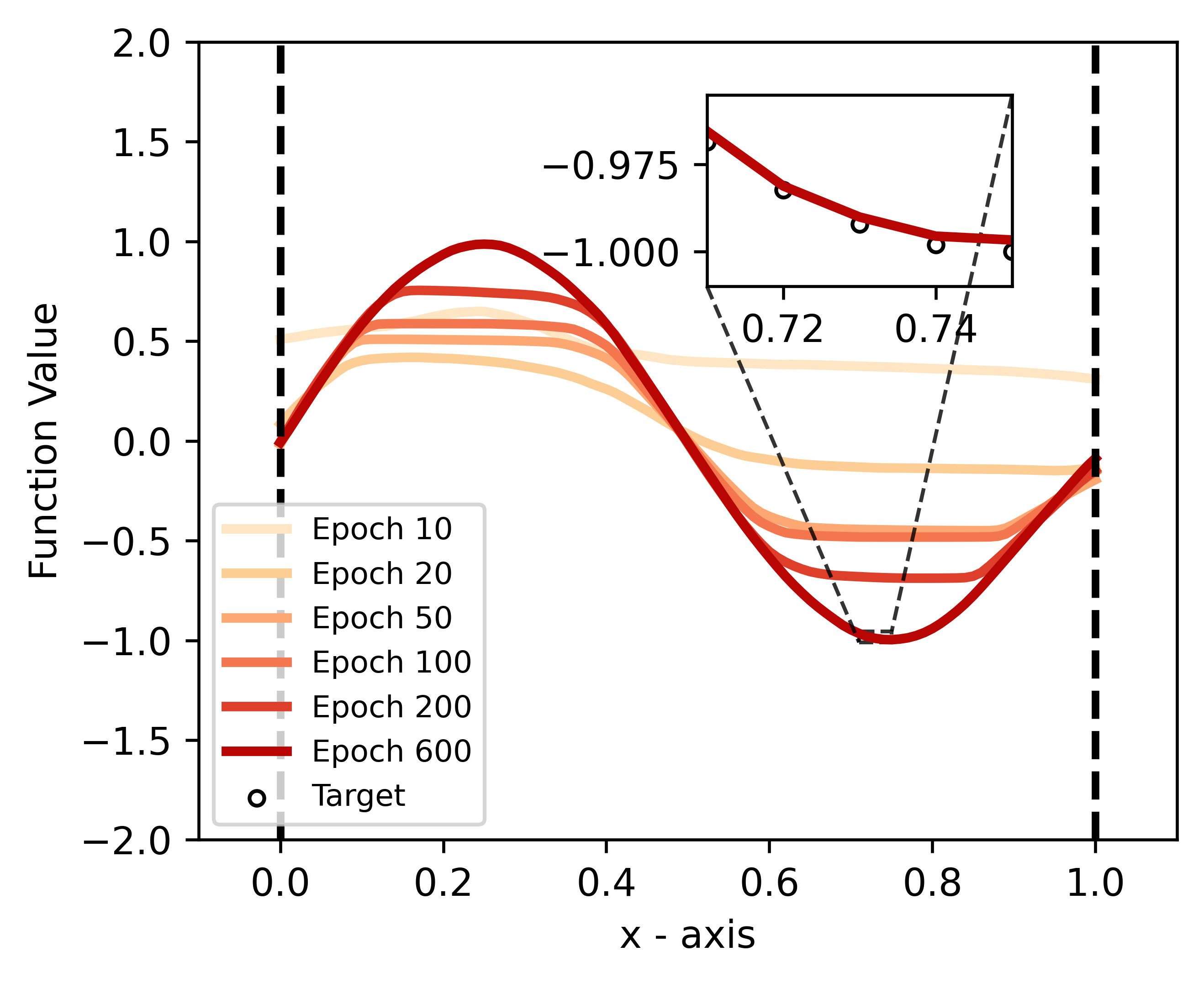
(a) Approximated function value.

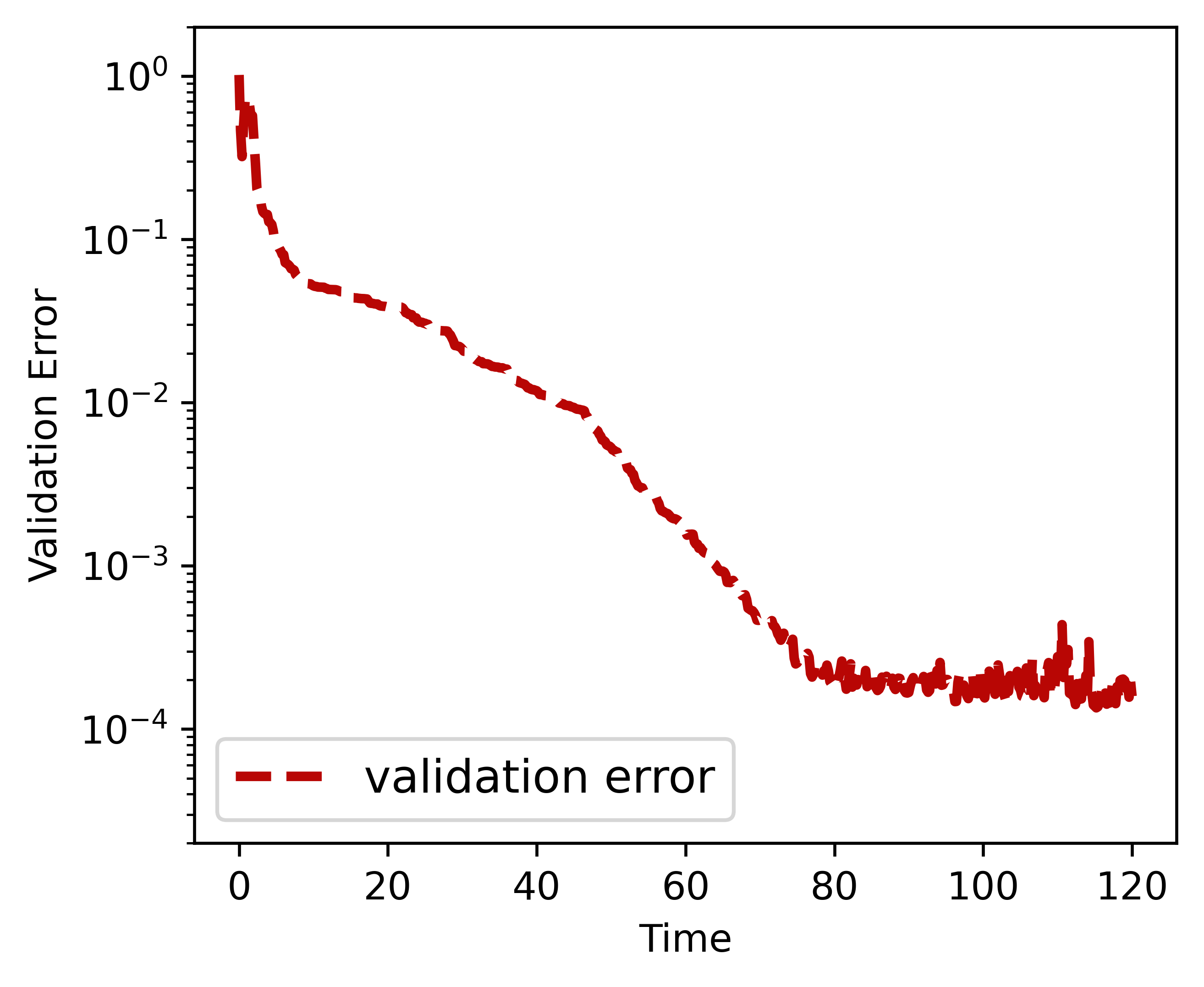
(b) Validation error in training.

Figure 1: (a) The approximated function value at different time: the colors from shallow to deep represents the number of outer iterations processed, epoch 10, 20, 50, 100, 200, 600 respectively; (b) The validation error at different training epochs.

5 Proofs

5.1 Proof of Propositions 1 and 4

Proof of Propositions 1 and 4  We only show Proposition 1 as the method is completely the same for the other proposition.

By Assumption 1 we have $\liminf_{x\to\infty}U(x)/\lvert x\rvert^{p}>0$. Then we can find $R$, $c>0$ such that $U(x)\geq c\lvert x\rvert^{p}$ for $\lvert x\rvert>R$. Choose a minimizing sequence $(m_{n})_{n\in\mathbb{N}}$ in the sense that $V^{\sigma}(m_{n})\searrow\inf_{m\in\mathcal{P}(\mathbb{R}^{d})}V^{\sigma}(m)$ when $n\to+\infty$. Then we have

$$\sup_{n\in\mathbb{N}}V^{\sigma}(m_{n}) \geq H(m_{n}|e^{-U})=\int m_{n}(x)\bigl{(}\log m_{n}(x)+U(x)\bigr{)}\,dx$$

$$=\biggl{(}\int_{\lvert x\rvert\leq R}+\int_{\lvert x\rvert>R}\biggr{)}m_{n}(x)\bigl{(}\log m_{n}(x)+U(x)\bigr{)}\,dx$$

$$\geq-\frac{c_{d}R^{d}}{e}+\operatorname*{ess\,inf}_{\lvert x\rvert\leq R}U(x)+\int_{\lvert x\rvert>R}m_{n}(x)\bigl{(}\log m_{n}(x)+U(x)\bigr{)}\,dx$$

$$\geq-\frac{c_{d}R^{d}}{e}+\operatorname*{ess\,inf}_{\lvert x\rvert\leq R}U(x)+\int_{\lvert x\rvert>R}m_{n}(x)\bigl{(}\log m_{n}(x)+c\lvert x\rvert^{p}\bigr{)}\,dx,$$

where the second inequality is due to $x\log x\geq-e^{-1}$ and $c_{d}$ denotes the volume of the $d$-dimensional unit ball.

Define $\tilde{Z}=\int_{\lvert x\rvert>R}\exp\bigl{(}-c|x|^{p}/2\bigr{)}\,dx$ and denote by $\tilde{g}$ the probability measure

$$\tilde{g}(dx)=\frac{\mathbf{1}_{|x|>R}}{\tilde{Z}}\exp\biggl{(}-\frac{c}{2}\lvert x\rvert^{p}\biggr{)}\,dx$$

supported on $\{\lvert x\rvert>R\}$. Using the fact that the relative entropy is always nonnegative, we have

$$\int_{\lvert x\rvert>R}m_{n}(x)\bigl{(}\log m_{n}(x)+c\lvert x\rvert^{p}\bigr{)}\,dx$$

$$=\int_{\lvert x\rvert>R}m_{n}(x)\biggl{(}\log m_{n}(x)+\frac{c}{2}\lvert x\rvert^{p}+\frac{c}{2}\lvert x\rvert^{p}\biggr{)}\,dx$$

$$=H(m_{n}|\tilde{g})-\log\tilde{Z}\int_{\lvert x\rvert>R}m_{n}(x)\,dx+\frac{c}{2}\int_{\lvert x\rvert>R}m_{n}(x)\lvert x\rvert^{p}\,dx$$

$$\geq-\lvert\log\tilde{Z}\rvert+\frac{c}{2}\int_{\lvert x\rvert>R}m_{n}(x)\lvert x\rvert^{p}\,dx.$$

Combining the two inequalities above, we obtain

$$\frac{c}{2}\int_{\lvert x\rvert>R}m_{n}(x)\lvert x\rvert^{p}\,dx\leq\lvert\log\tilde{Z}\rvert+\frac{c_{d}R^{d}}{e}-\operatorname*{ess\,inf}_{\lvert x\rvert<R}U(x)+\sup_{n\in\mathbb{N}}V^{\sigma}(m_{n}),$$

which implies

$$\sup_{n\in\mathbb{N}}\lVert m_{n}\rVert^{p}_{p}=\sup_{n\in\mathbb{N}}\int m_{n}(x)\lvert x\rvert^{p}\,dx<+\infty,$$

that is, the $p$-moment of the minimizing sequence is uniformly bounded. So the sequence $(m_{n})_{n\in\mathbb{N}}$ is tight and $m_{n}\to m^{*}$ weakly for some $m^{*}\in\mathcal{P}(\mathbb{R}^{d})$ along a subsequence. Applying the following lemma, whose proof is postponed, we obtain $m^{*}\in\mathcal{P}_{p}(\mathbb{R}^{d})$.

Lemma 13 (“Fatou’s lemma” for weak convergence of measure)

Let $X$ be a metric space, $f:X\to\mathbb{R}_{+}$ be nonnegative continuous function and $(m_{n})_{n\in\mathbb{N}}$ be a sequence of probability measures on $X$. If $m_{n}$ converges to another probability measure $m$ weakly, then

$$\int_{X}f\,dm\leq\liminf_{n\to+\infty}\int_{X}f\,dm_{n}.$$

Since the relative entropy is weakly lower-semicontinuous, the entropy of $m^{*}$ satisfies

$$H(m^{*}|g)\leq\liminf_{n\to+\infty}H(m_{n}|g).$$

We show the regular part satisfies $\lim_{n\to+\infty}F(m_{n})=F(m^{*})$. Indeed, by the definition of functional derivative, we have

$$\bigl{|}F(m_{n})-F(m^{*})\bigr{|}\leq\int_{0}^{1}\biggl{|}\int_{\mathbb{R}^{d}}\frac{\delta F}{\delta m}(m_{\lambda,n},x)\,(m_{n}-m)(dx)\biggr{|}\,d\lambda$$

where $m_{\lambda,n}\coloneqq(1-\lambda)m_{n}+\lambda m$. For every $\lambda\in[0,1]$, we have

$$\biggl{|}\int_{\mathbb{R}^{d}}\frac{\delta F}{\delta m}(m_{\lambda,n},x)\,(m_{n}-m^{*})(dx)\biggr{|}\\ \leq\biggl{|}\int_{\mathbb{R}^{d}}\frac{\delta F}{\delta m}(m^{*},x)\,(m_{n}-m^{*})(dx)\biggr{|}+\int_{\mathbb{R}^{d}}\biggl{|}\frac{\delta F}{\delta m}(m_{n},x)-\frac{\delta F}{\delta m}(m^{*},x)\biggr{|}\,(m_{n}+m^{*})(dx).$$

Since $\frac{\delta F}{\delta m}(m^{*},\cdot)$ is a bounded continuous function, the weak convergence $m_{n}\to m^{*}$ implies

$$\lim_{n\to+\infty}\biggl{|}\int_{\mathbb{R}^{d}}\frac{\delta F}{\delta m}(m^{*},x)\,(m_{n}-m^{*})(dx)\biggr{|}=0.$$

It remains to show the second term also converges to $0$. Since the convergence $\frac{\delta F}{\delta m}(m_{n},x)\to\frac{\delta F}{\delta m}(m^{*},x)$ is uniform for $\lvert x\rvert<R$ for every $R>0$, we have

$$\lim_{n\to+\infty}\int_{\lvert x\rvert\leq R}\biggl{|}\frac{\delta F}{\delta m}(m_{n},x)-\frac{\delta F}{\delta m}(m^{*},x)\biggr{|}\,(m_{n}+m^{*})(dx)=0.$$

Consequently,

$$\limsup_{n\to+\infty} \int_{\mathbb{R}^{d}}\biggl{|}\frac{\delta F}{\delta m}(m_{n},x)-\frac{\delta F}{\delta m}(m^{*},x)\biggr{|}\,(m_{n}+m^{*})(dx)$$

$$=\limsup_{n\to+\infty}\biggl{(}\int_{\lvert x\rvert\leq R}+\int_{\lvert x\rvert>R}\biggr{)}\biggl{|}\frac{\delta F}{\delta m}(m_{n},x)-\frac{\delta F}{\delta m}(m^{*},x)\biggr{|}\,(m_{n}+m^{*})(dx)$$

$$\leq\limsup_{n\to+\infty}\int_{\lvert x\rvert>R}\biggl{|}\frac{\delta F}{\delta m}(m_{n},x)-\frac{\delta F}{\delta m}(m^{*},x)\biggr{|}\,(m_{n}+m^{*})(dx)$$

$$\leq M_{F}\limsup_{n\to+\infty}\int_{\lvert x\rvert>R}(m_{n}+m^{*})(dx)$$

$$=M_{F}\limsup_{n\to+\infty}\bigl{(}m^{*}(\{\lvert x\rvert>R\})+m_{n}(\{\lvert x\rvert>R\})\bigr{)}=0$$

by tightness of the sequence $(m_{n})_{n\in\mathbb{N}}$. Finally, using the boundedness

$$\biggl{|}\int_{\mathbb{R}^{d}}\frac{\delta F}{\delta m}(m_{\lambda,n},x)\,(m_{n}-m)(dx)\biggr{|}\leq 2M_{F},$$

we can apply the dominated convergence theorem and show that when $n\to+\infty$,

$$\int_{0}^{1}\biggl{|}\int_{\mathbb{R}^{d}}\frac{\delta F}{\delta m}(m_{\lambda,n},x)\,(m_{n}-m)(dx)\biggr{|}\,d\lambda\to 0.$$

Summing up, we have obtained a measure $m^{*}\in\mathcal{P}_{p}(\mathbb{R}^{d})$ such that

$$V^{\sigma}(m^{*})=F(m^{*})+\frac{\sigma^{2}}{2}H(m^{*})\\ \leq\liminf_{n\to+\infty}F(m_{n})+\frac{\sigma^{2}}{2}H(m_{n})=\liminf_{n\to+\infty}V^{\sigma}(m_{n})=\inf_{m\in\mathcal{P}(\mathbb{R}^{d})}V^{\sigma}(m).$$

This completes the proof.  

Proof of Lemma 13  By the construction of Lebesgue integral, for every positive measure $\mu\in\mathcal{P}(X)$, we have

$$\int_{X}f\,d\mu=\sup_{M\geq 0}\int_{X}f\wedge M\,d\mu.$$

Therefore,

$$\int_{X}f\,dm =\sup_{M\geq 0}\int_{X}f\wedge M\,dm=\sup_{M\geq 0}\liminf_{n\to+\infty}\int_{X}f\wedge M\,dm_{n}=\sup_{M\geq 0}\sup_{n}\inf_{k>n}\int_{X}f\wedge M\,dm_{k}$$

$$\leq\sup_{n}\inf_{k>n}\sup_{M\geq 0}\int_{X}f\wedge M\,dm_{k}=\liminf_{n\to+\infty}\sup_{M\geq 0}\int_{X}f\wedge M\,dm_{n}=\liminf_{n\to+\infty}\int_{X}f\,dm_{n},$$

where the inequality is due to $\sup\inf\leq\inf\sup$.  

5.2 Proof of Proposition 7

We prove several technical results before proceeding to the proof of Proposition 7.

Proposition 14

Suppose Assumption 1 holds. For every $m\in\mathcal{P}_{p}(\mathbb{R}^{d})$, the measure $\hat{m}$ determined by

$$\hat{m}=\frac{1}{Z_{m}}\exp\biggl{(}-\frac{\delta F}{\delta m}(m,x)-U(x)\biggr{)},$$ (20)

where $Z_{m}$ is the normalization constant, is well defined and belongs to $\mathcal{P}_{p}(\mathbb{R}^{d})$. Moreover, there exists constants $c$, $C$ with $0<c<1<C<+\infty$ such that for every $m\in\mathcal{P}_{p}(\mathbb{R}^{d})$ and every $x\in\mathbb{R}^{d}$,

$$ce^{-U(x)}\leq\hat{m}(x)\leq Ce^{-U(x)},$$ (21)

Finally, there exists a constant $L>0$ such that for every $m$, $m^{\prime}\in\mathcal{P}_{p}(\mathbb{R}^{d})$ and every $x\in\mathbb{R}^{d}$,

$$\lvert\hat{m}(x)-\hat{m}^{\prime}(x)\rvert\leq L\mathcal{W}_{p}(m,m^{\prime})e^{-U(x)}.$$ (22)

Proof  Using (11), we have

$$\exp\biggl{(}-\frac{2}{\sigma^{2}}M_{F}-U(x)\biggr{)}\leq\exp\biggl{(}-\frac{2}{\sigma^{2}}\frac{\delta F}{\delta m}(m,x)-U(x)\biggr{)}\leq\exp\biggl{(}\frac{2}{\sigma^{2}}M_{F}-U(x)\biggr{)},$$ (23)

and

$$\exp\biggl{(}-\frac{2M_{F}}{\sigma^{2}}\biggr{)}Z_{0}\\ =\int_{\mathbb{R}^{d}}\exp\biggl{(}-\frac{2}{\sigma^{2}}M_{F}-U(x)\biggr{)}dx\leq Z_{m}\leq\int_{\mathbb{R}^{d}}\exp\biggl{(}\frac{2}{\sigma^{2}}M_{F}-U(x)\biggr{)}\,dx\\ =\exp\biggl{(}\frac{2M_{F}}{\sigma^{2}}\biggr{)}Z_{0},$$ (24)

Thus $\hat{m}$ is well defined and (21) holds with constant $C=c^{-1}=\exp\bigl{(}4M_{F}\sigma^{-2}\bigr{)}$. Consequently,

$$\int_{\mathbb{R}^{d}}\lvert x\rvert^{p}\,\hat{m}(dx)\leq\int_{\mathbb{R}^{d}}\lvert x\rvert^{p}\hat{m}(x)\,dx\leq\int_{\mathbb{R}^{d}}\lvert x\rvert^{p}Ce^{-U(x)}\,dx<+\infty,$$

that is, $\hat{m}\in\mathcal{P}_{p}(\mathbb{R}^{d})$.

Meanwhile, using the elementary inequality $\lvert e^{x}-e^{y}\rvert\leq e^{x\vee y}\lvert x-y\rvert$, we have

$$\biggl{|}\exp\biggl{(}-\frac{2}{\sigma^{2}}\frac{\delta F}{\delta m}(m,x)-U(x)\biggr{)}-\exp\biggl{(}-\frac{2}{\sigma^{2}}\frac{\delta F}{\delta m}(m^{\prime},x)-U(x)\biggr{)}\biggr{|}\\ \leq\frac{2}{\sigma^{2}}\exp\biggl{(}\frac{2M_{F}}{\sigma^{2}}\biggr{)}\mathcal{W}_{p}(m,m^{\prime})\exp\bigl{(}-U(x)\bigr{)}.$$

Integrating the previous inequality with respect to $x$, we obtain

$$\lvert Z-Z^{\prime}\rvert\leq\frac{2}{\sigma^{2}}\exp\biggl{(}\frac{2M_{F}}{\sigma^{2}}\biggr{)}\mathcal{W}_{p}(m,m^{\prime})Z_{0}.$$

Using the bounds (23) and (24), we obtain the Lipschitz continuity (22).  

The Lipschitz continuity (22) implies the Hölder continuity of $m\mapsto\hat{m}$.

Corollary 15

Suppose Assumption 1 holds. Then the mapping $\Phi:\mathcal{P}_{p}(\mathbb{R}^{d})\to\mathcal{P}_{p}(\mathbb{R}^{d})$ is $1/p$-Hölder continuous.

Before proving the corollary we show a lemma bounding the Wasserstein (coupling) distance between two probability measures by the $L^{\infty}$ distance between their density functions.

Lemma 16

Let $(X,d)$ be a metric space and $\mu$ be a Borel probability measure on $X$. Consider the space of positive integrable functions with respect to $\mu$,

$$L^{\infty}_{+,1}(\mu)\coloneqq\biggl{\{}f:X\to\mathbb{R}~{}\text{Borel measurable}:f\geq 0,\int f\,d\mu=1\biggr{\}}.$$

Equip $L^{\infty}_{+,1}(\mu)$ with the usual $L^{\infty}$ distance. Suppose for some $p\geq 1$ and some $x_{0}\in X$, we have $C_{\mu,p}\coloneqq\int_{X}d(x,x_{0})^{p}\,\mu(dx)<+\infty$. Then there exists a constant $L_{\mu,p}>0$ such that for every $f$, $g\in L^{\infty}_{+,1}(\mu)$,

$$\mathcal{W}_{p}(f\,\mu,g\,\mu)\leq L_{\mu,p}\lVert f-g\rVert^{1/p}_{L^{\infty}},$$

where $f\,\mu$ is the probability measure determined by $(f\,\mu)(A)\coloneqq\int_{A}f\,d\mu$ and similarily for $g$.

Proof  Construct the following coupling $\pi$ between $f\,\mu$, $g\,\mu$:

$$\pi \coloneqq\pi_{1}+\pi_{2},$$

$$\pi_{1}(dx\,dy) \coloneqq(f\wedge g)(x)\,\mu_{\Delta}(dx\,dy),$$

$$\pi_{2}(dx\,dy) \coloneqq\biggl{(}\int(f-g)_{+}(x)\mu(dx)\biggr{)}^{-1}(f-g)_{+}(x)(g-f)_{+}(y)\,\mu(dx)\,\mu(dy).$$

Here $\mu_{\Delta}$ is the measure supported on the diagonal $\Delta\coloneqq\{(x,x):x\in X\}\subset X\times X$ such that $\mu_{\Delta}(A\times A)=\mu(A)$. One readily verifies that the projection mappings to the first and second variables, denoted by $X$, $Y$ respectively, satisfy

$$X_{\#}\pi_{1}=Y_{\#}\pi_{1} =(f\wedge g)\,\mu,$$

$$X_{\#}\pi_{2} =(f-g)_{+}\,\mu,$$

$$Y_{\#}\pi_{2} =(g-f)_{+}\,\mu$$

Hence $X_{\#}\pi=f\,\mu$, $Y_{\#}\pi=g\,\mu$ and $\pi$ is indeed a coupling between $f\,\mu$, $g\,\mu$.

By the definition of Wasserstein distance, we obtain

$$\mathcal{W}_{p}(f\,\mu,g\,\mu)^{p}\leq\int_{X\times X}d(x,y)^{p}\pi_{1}\,(dx\,dy)+\int_{X\times X}d(x,y)^{p}\pi_{2}\,(dx\,dy)\\ =\biggl{(}\int(f-g)_{+}\,\mu\biggr{)}^{-1}\int_{X\times X}(f-g)_{+}(x)(g-f)_{+}(y)d(x,y)^{p}\,\mu(dx)\,\mu(dy).$$

Using triangle inequality $d(x,y)^{p}\leq C_{p}\bigl{(}d(x,x_{0})^{p}+d(y,x_{0})^{p}\bigr{)}$ and exchanging $x$, $y$, the last term is again bounded by

$$\biggl{(}\int(f-g)_{+}\,\mu\biggr{)}^{-1}\int_{X\times X}C_{p}\bigl{(}d(x,x_{0})^{p}+d(y,x_{0})^{p}\bigr{)}(f-g)_{+}(x)(g-f)_{+}(y)\,\mu(dx)\,\mu(dy)$$

$$=\frac{C_{p}}{\int(f-g)_{+}\,\mu}\int_{X\times X}d(x,x_{0})^{p}\biggl{[}(f-g)_{+}(x)(g-f)_{+}(y)$$

$$\hphantom{=\frac{C_{p}}{\int(f-g)_{+}\,\mu}\int_{X\times X}d(x,x_{0})^{p}\biggl{[}}\quad+(g-f)_{+}(x)(f-g)_{+}(y)\biggr{]}\,\mu(dx)\,\mu(dy)$$

$$=C_{p}\int_{X}d(x,x_{0})^{p}|f-g|(x)\,\mu(dx)\leq C_{p}C_{\mu,p}\|f-g\|_{L^{\infty}}.$$

The Hölder constant is then given by $L_{\mu,p}=(C_{p}C_{\mu,p})^{1/p}$.  

Remark 17

The Hölder exponent $1/p$ in the inequality is sharp. Consider the example: $\mu=\mathrm{Leb}_{[0,1]}$, $f=(1+\varepsilon)\mathbf{1}_{\left[0,\frac{1}{2}\right)}+(1-\varepsilon)\mathbf{1}_{\left[\frac{1}{2},1\right]}$, $g=(1-\varepsilon)\mathbf{1}_{[0,\frac{1}{2})}+(1+\varepsilon)\mathbf{1}_{\left[\frac{1}{2},1\right]}$. Then the $\mathcal{W}_{p}$ distance between $f\mu$, $g\mu$ is of order $\varepsilon^{1/p}$ when $\varepsilon\to 0$.

Proof of Corollary 15  Applying Lemma 16 with $\mu(dx)=e^{-U(x)}\,dx$, we obtain

$$\mathcal{W}_{p}(\hat{m}_{1},\hat{m}_{2})\leq L\biggl{\|}\frac{\hat{m}_{1}(x)}{e^{-U(x)}}-\frac{\hat{m}_{2}(x)}{e^{-U(x)}}\biggr{\|}_{L^{\infty}}^{1/p},$$

while by (22) we have

$$\biggl{\|}\frac{\hat{m}_{1}(x)}{e^{-U(x)}}-\frac{\hat{m}_{2}(x)}{e^{-U(x)}}\biggr{\|}_{L^{\infty}}\leq L\mathcal{W}_{p}(m_{1},m_{2}).$$

The Hölder continuity follows.  

Proof of Proposition 7  Existence. We will use Schauder’s fixed point theorem. To this end, fix $T>0$, let $m_{0}\in\mathcal{P}_{p}$ be the initial value and denote $X=C([0,T];\mathcal{W}_{p})$. Let $\mathbf{T}:X\to X$ be the mapping determined by

$$\mathbf{T}[m]_{t}\coloneqq\int_{0}^{t}\alpha e^{-\alpha(t-s)}\,\hat{m}_{s}\,ds+e^{-\alpha t}\,m_{0}=\int_{0}^{t}\alpha e^{-\alpha(t-s)}\,\Phi(m_{s})\,ds+e^{-\alpha t}\,m_{0},\quad t\in[0,T].$$ (25)

We verify indeed $\mathbf{T}[m]\in X$, i.e. $\mathbf{T}[m]_{t}\in\mathcal{P}_{p}$ for every $t\in[0,T]$, and $t\mapsto\mathbf{T}[m]_{t}$ is continuous with respect to $\mathcal{W}_{p}$. This first claim follows from the fact that $\mathbf{T}[m]_{t}$ is a convex combination of elements in $\mathcal{P}_{p}$, as we have shown $\hat{m}_{s}=\Phi(m_{s})\in\mathcal{P}_{p}(\mathbb{R}^{d})$. The second claim follows from

$$\mathcal{W}_{p}(\mathbf{T}[m]_{t+\delta},\mathbf{T}[m]_{t})^{p}\leq\alpha\int_{0}^{\delta}e^{-\alpha(\delta-s)}\mathcal{W}_{p}(\hat{m}_{s},m_{t})^{p}\,ds\\ \leq C(1-e^{-\alpha\delta})\bigl{(}{\textstyle\sup}_{\hat{m}\in\operatorname{Im}\Phi}M_{p}(\hat{m})+M_{p}(\mathbf{T}[m]_{t})\bigr{)}.$$ (26)

Next we show the compactness of the mapping $\mathbf{T}$. Setting $t=0$ in the previous equation and letting $\delta$ vary in $[0,T]$, we obtain

$$\sup_{m\in X}\sup_{t\in[0,T]}M_{p}\bigl{(}\mathbf{T}[m]_{t}\bigr{)}\leq C.$$

Plugging this back to (26), we have

$$\sup_{m\in X,0\leq t<t+\delta\leq T}\mathcal{W}_{p}\bigl{(}\mathbf{T}[m]_{t+\delta},\mathbf{T}[m]_{t}\bigr{)}\leq C\delta^{1/p}.$$ (27)

From (11) one knows that $\operatorname{Im}\Phi$ forms a precompact set in $\mathcal{P}_{p}$, and since $X_{t}\coloneqq\{\mathbf{T}[m]_{t}:m\in X\}$ lies in the convex combination of $\operatorname{Im}\Phi$ and $\{m_{0}\}$, $X_{t}$ is also precompact. Then by the Arzelà–Ascoli theorem, $\operatorname{Im}\mathbf{T}=\mathbf{T}[X]$ is a precompact set. In other words, $\mathbf{T}$ is a compact mapping. We use Schauder’s theorem to conclude that $\mathbf{T}$ admits a fixed point, i.e. (16) admits at least one solution in $X$.

Wellposedness when $p=1$. The mapping $\Phi$ is Lipschitz in this case. The wellposedness follows from standard Picard–Lipschitz arguments.

Pointwise solution. By definition, $\hat{m}_{t}$ admits the density function

$$\hat{m}_{t}(x)=\frac{1}{Z_{t}}\exp\biggl{(}-\frac{2}{\sigma^{2}}\frac{\delta F}{\delta m}(m_{t},x)-U(x)\biggr{)},$$

where $Z_{t}\coloneqq\int_{\mathbb{R}^{d}}\exp\bigl{(}-\frac{2}{\sigma^{2}}\frac{\delta F}{\delta m}(m_{t},x)-U(x)\bigr{)}\,dx$ is the normalization constant. The functional derivative $\frac{\delta F}{\delta m}(m_{t},x)$ is continuous in $t$ by the continuities of $t\mapsto m_{t}$ and $m\mapsto\frac{\delta F}{\delta m}(m,x)$, and is bounded for every $t\geq 0$. By the dominated convergence theorem, both $\exp\bigl{(}-\frac{2}{\sigma^{2}}\frac{\delta F}{\delta m}(m_{t},x)-U(x)\bigr{)}$ and $Z_{t}$ are continuous in $t$ and bounded. Hence $t\mapsto\hat{m}_{t}(x)$ is continuous and bounded uniformly in $x$. Suppose now the initial value $m_{0}$ has density $m_{0}(x)$. Define the density of $m_{t}$ according to the Duhamel’s formula (25):

$$m_{t}(x)\coloneqq\int_{0}^{t}\alpha e^{-\alpha(t-s)}\hat{m}_{s}(x)\,ds+e^{-\alpha t}m_{0}(x),\quad\text{for}~{}x\in\mathbb{R}^{d}.$$ (28)

By definition $m_{t}(x)$ defined by (28) is indeed the density of $m_{t}$ solving the time dynamics (16), and is automatically continuous in $t$. Since $\alpha e^{-\alpha(t-s)}\hat{m}_{s}(x)$ in (28) is continuous and bounded in $s$ for every $t\geq 0$, the density $m_{t}(x)$ is $C^{1}$ in $t$ and satisfies the pointwise equality (17).  

We also obtain a density bound that will be used in the following.

Corollary 18

Suppose Assumption 1 holds. There exist constants $c$, $C>0$, depending only on $F$ and $U$, such that

$$m_{t}(x) \geq(1-e^{-\alpha t})ce^{-U(x)},$$ (29)

$$m_{t}(x) \leq(1-e^{-\alpha t})Ce^{-U(x)}+e^{-\alpha t}m_{0}(x),$$ (30)

for every $x\in\mathbb{R}^{d}$.

Proof  For all $\hat{m}\in\operatorname{Im}\Phi$, we have

$$\hat{m}(x)\geq ce^{-U(x)}.$$

Then by the definition of density (28), we have

$$m_{t}(x) \geq\int_{0}^{t}\alpha e^{-\alpha(t-s)}\hat{m}_{s}(x)\,ds$$

$$\geq ce^{-U(x)}\int_{0}^{t}\alpha e^{-\alpha(t-s)}\hat{m}_{s}(x)\,ds$$

$$=(1-e^{-\alpha t})ce^{-U(x)}.$$

The proof for the upper bound is similar.  

5.3 Proof of Theorem 9

As it is important to our proof of Theorem 9, we single out the derivative in time result in the following proposition and prove it before tackling the other parts of the theorem.

Proposition 19

Suppose Assumptions 1 and 2 holds, and let $(m_{t})_{t\geq 0}$ be a solution to (16) in $\mathcal{W}_{p}$. Then for every $t>0$,

$$\frac{dV^{\sigma}(m_{t})}{dt}=-\frac{\alpha\sigma^{2}}{2}\bigl{(}H(m_{t}|\hat{m}_{t})+H(\hat{m}_{t}|m_{t})\bigr{)}.$$ (31)

Before proving the proposition, we show a lemma on the uniform integrability of $m_{t}$ and $\hat{m}_{t}$.

Lemma 20

Fix $s>0$. Under the conditions of the previous proposition, there exist integrable functions $f$, $g$ such that for every $t\in[s,+\infty)$ and every $x\in\mathbb{R}^{d}$,

$$g(x)\leq\log\frac{m_{t}(x)}{e^{-U(x)}}\bigl{(}\hat{m}_{t}(x)-m_{t}(x)\bigr{)}\leq f(x).$$

Proof  We first deal with the first term $\log\frac{m_{t}(x)}{e^{-U(x)}}\hat{m}_{t}(x)$. Using the bounds (29), (30) we have

$$\log\frac{m_{t}(x)}{e^{-U(x)}}\hat{m}_{t}(x) \geq\log\frac{(1-e^{-\alpha t})ce^{-U(x)}}{e^{-U(x)}}\hat{m}_{t}(x)=\log\bigl{(}(1-e^{-\alpha t})c\bigr{)}\hat{m}_{t}(x)$$

$$\geq\log\bigl{(}(1-e^{-\alpha s}\bigr{)}c)\hat{m}_{t}(x)\geq\log\bigl{(}(1-e^{-\alpha s})c\bigr{)}Ce^{-U(x)}\eqqcolon g_{1}(x).$$

Here we shrink the constant $c$ if necessary so that $c<1$ and in the last inequality the coefficient $\log\bigl{(}(1-e^{-\alpha s})c\bigr{)}$ is negative. Now we upper bound $\log\frac{m_{t}(x)}{e^{-U(x)}}\hat{m}_{t}(x)$. We have

$$\log\frac{m_{t}(x)}{e^{-U(x)}} \leq\log\biggl{(}e^{-\alpha t}\frac{m_{0}(x)}{e^{-U(x)}}+\int_{0}^{t}\alpha e^{-\alpha(t-s)}\frac{\hat{m}_{s}(x)}{e^{-U(x)}}\,ds\biggr{)}$$

$$\leq\log\biggl{(}e^{-\alpha t}\frac{m_{0}(x)}{e^{-U(x)}}+C\int_{0}^{t}\alpha e^{-\alpha(t-s)}\,ds\biggr{)}=\log\biggl{(}e^{-\alpha t}\frac{m_{0}(x)}{e^{-U(x)}}+C(1-e^{-\alpha t})\biggr{)}$$

$$\leq\log\bigl{(}(1-e^{-\alpha t})C\bigr{)}+\frac{e^{-\alpha t}}{C(1-e^{-\alpha t})}\frac{m_{0}(x)}{e^{-U(x)}}\leq\log C+C_{s}\frac{m_{0}(x)}{e^{-U(x)}}.$$

Here in the third inequality we used the elementary inequality $\log(x+y)\leq\log x+\frac{y}{x}$ for real $x$, $y$, and in the last line we maximize over $t\geq s$ and set $C_{s}=e^{-\alpha s}\bigl{(}C(1-e^{-\alpha s})\bigr{)}^{-1}$. Therefore,

$$\log\frac{m_{t}(x)}{e^{-U(x)}}\hat{m}_{t}(x) \leq\biggl{(}\log C+C_{s}\frac{m_{0}(x)}{e^{-U(x)}}\biggr{)}\hat{m}_{t}(x)\leq\biggl{(}\log C+C_{s}\frac{m_{0}(x)}{e^{-U(x)}}\biggr{)}Ce^{-U(x)}$$

$$=\log C\cdot Ce^{-U(x)}+C_{s}Cm_{0}(x)\eqqcolon f_{1}(x).$$

Now consider the second term $\log\frac{m_{t}(x)}{e^{-U(x)}}m_{t}(x)$. Applying Jensen’s inequality to the Duhamel formula (28), we have

$$\log\frac{m_{t}(x)}{e^{-U(x)}}m_{t}(x) \leq e^{-\alpha t}\log\frac{m_{0}(x)}{e^{-U(x)}}m_{0}(x)+\int_{0}^{t}\alpha e^{-\alpha(t-s)}\log\frac{\hat{m}_{s}(x)}{e^{-U(x)}}\hat{m}_{s}(x)\,dt$$

$$\leq e^{-\alpha t}\log\frac{m_{0}(x)}{e^{-U(x)}}m_{0}(x)+\int_{0}^{t}\alpha e^{-\alpha(t-s)}\log C\cdot\hat{m}_{s}(x)\,dt$$

$$\leq e^{-\alpha t}\log\frac{m_{0}(x)}{e^{-U(x)}}m_{0}(x)+\int_{0}^{t}\alpha e^{-\alpha(t-s)}\log C\cdot Ce^{-U(x)}\,dt$$

$$\leq\biggl{(}\log\frac{m_{0}(x)}{e^{-U(x)}}m_{0}(x)\biggr{)}_{+}+\log C\cdot Ce^{-U(x)}\eqqcolon-g_{2}(x)$$

In the second and third inequality we use consecutively the bound $\hat{m}(x)\leq Ce^{-U(x)}$ with $C>1$. For the lower bound of the second term we note

$$\log\frac{m_{t}(x)}{e^{-U(x)}}m_{t}(x)=\log\frac{m_{t}(x)}{e^{-U(x)}}\cdot\frac{m_{t}(x)}{e^{-U(x)}}e^{-U(x)}\geq-\frac{1}{e}e^{-U(x)}\eqqcolon-f_{2}(x)$$

The proof is complete by letting $f=f_{1}+f_{2}$ and $g=g_{1}+g_{2}$.  

Proof of Proposition 19  Thanks to the lemma above, we can apply the dominated convergence theorem to differentiate $t\mapsto V^{\sigma}(m_{t})$ and obtain

$$\frac{dH(m_{t})}{dt}=\alpha\int_{\mathbb{R}^{d}}\bigl{(}\log m_{t}(x)+U(x)\bigr{)}\bigl{(}\hat{m}_{t}(x)-m_{t}(x)\bigr{)}\,dx.$$

For the regular term $F(m_{t})$, by the definition of functional derivative, we have

$$F(m_{t+\delta})-F(m_{t})=\int_{0}^{1}\int_{\mathbb{R}^{d}}\frac{\delta F}{\delta m}(m_{t+u\delta},x)\bigl{(}m_{t+\delta}(x)-m_{t}(x)\bigr{)}\,dx\,du.$$

Applying again the dominated convergence theorem, the derivative reads

$$\frac{dV^{\sigma}(m_{t})}{dt} =\alpha\int_{\mathbb{R}^{d}}\biggl{(}\frac{\delta F}{\delta m}(m_{t},x)+\frac{\sigma^{2}}{2}\log m_{t}(x)+\frac{\sigma^{2}}{2}U(x)\biggr{)}\bigl{(}\hat{m}_{t}(x)-m_{t}(x)\bigr{)}\,dx$$

$$=\alpha\int_{\mathbb{R}^{d}}\biggl{(}C_{t}+\frac{\sigma^{2}}{2}\log m_{t}(x)-\frac{\sigma^{2}}{2}\log\hat{m}_{t}(x)\biggr{)}\bigl{(}\hat{m}_{t}(x)-m_{t}(x)\bigr{)}\,dx$$

$$=\alpha\int_{\mathbb{R}^{d}}\biggl{(}\frac{\sigma^{2}}{2}\log m_{t}(x)-\frac{\sigma^{2}}{2}\log\hat{m}_{t}(x)\biggr{)}\bigl{(}\hat{m}_{t}(x)-m_{t}(x)\bigr{)}\,dx$$

$$=-\frac{\alpha\sigma^{2}}{2}\bigl{(}H(m_{t}|\hat{m}_{t})+H(\hat{m}_{t}|m_{t})\bigr{)},$$

where in the second line we use the first-order condition for $\hat{m}_{t}$ and $C_{t}$ is a constant that may depend on $t$.  

Remark 21

The result of Proposition 19 implies

• $\int_{0}^{+\infty}\bigl{(}H(m_{t}|\hat{m}_{t})+H(\hat{m}_{t}|m_{t})\bigr{)}\,dt<+\infty$;

• The derivative $\frac{dV^{\sigma}(m_{t})}{dt}$ vanishes if and only if $m_{t}=\hat{m}_{t}$, i.e. the dynamics reaches a stationary point.

Proof of Theorem 9  Our strategy of proof is as follows. First we show that, by the (pre-)compactness of the flow $(m_{t})_{t\geq 0}$ in a suitable Wasserstein space, the flow converges up to an extraction of subsequence. Then we prove by a monotonicity argument the convergence holds true without extraction. Finally we study the convergence of the density functions and prove the convergence of value function by the dominated convergence theorem.

According to the Duhamel’s formula (25), the measure $m_{t}$ is a (weighted) linear combination of the initial value $m_{0}$ and the best responses $\hat{m}_{s}$. Since there exists some $p^{\prime}>p$ such that $m_{0}\in\mathcal{P}_{p^{\prime}}(\mathbb{R}^{d})$, we obtain by the triangle inequality

$$\|m_{t}\|_{p^{\prime}}^{p^{\prime}}\leq e^{-\alpha t}\|m_{0}\|_{p^{\prime}}^{p^{\prime}}+(1-e^{-\alpha t})\sup_{0\leq s\leq t}\|\hat{m}_{s}\|_{p^{\prime}}^{p^{\prime}}\\ \leq\|m_{0}\|_{p^{\prime}}^{p^{\prime}}+\sup_{m\in\mathcal{P}_{p}(\mathbb{R}^{d})}\|\Phi(m)\|_{p^{\prime}}^{p^{\prime}}\leq\|m_{0}\|_{p^{\prime}}^{p^{\prime}}+C\int_{\mathbb{R}^{d}}x^{p^{\prime}}e^{-U(x)}\,dx.$$

Thus the flow $(m_{t})_{t\geq 0}$ in precompact in $\mathcal{P}_{p}(\mathbb{R}^{d})$ and the set of limit points,

$$w(m_{0})\coloneqq\{m\in\mathcal{P}_{p}(\mathbb{R}^{d}):\exists t_{n}\to+\infty~{}\text{such that}~{}m_{t_{n}}\to m\},$$

is nonempty. We now show that $w(m_{0})$ is the singleton $\{m^{*}\}$ and therefore $m_{t}\to m^{*}$ in $\mathcal{W}_{p}$. Pick $m\in w(m_{0})$ and let $(t_{n})_{n\in\mathbb{N}}$ be an increasing sequence such that $t_{n}\to+\infty$ and $m_{t_{n}}\to m$. Extracting a subsequence if necessary, we may suppose $t_{n+1}-t_{n}\geq 1$ for $n\in\mathbb{N}$. Proposition 19 implies for every $t$, $s$ such that $t>s\geq 0$,

$$V^{\sigma}(m_{s})-V^{\sigma}(m_{t})=\int_{s}^{t}\bigl{(}H(m_{u}|\hat{m}_{u})+H(\hat{m}_{u}|m_{u})\bigr{)}\,du.$$

Consequently,

$$V^{\sigma}(m_{0}) \geq V^{\sigma}(m_{t_{0}})-V^{\sigma}(m_{t_{n}})$$

$$\geq\sum_{k=0}^{n-1}\int_{t_{k}}^{t_{k}+1}\bigl{(}H(m_{u}|\hat{m}_{u})+H(\hat{m}_{u}|m_{u})\bigr{)}\,du$$

$$\geq\sum_{k=0}^{n-1}\int_{0}^{1}\bigl{(}H(m_{t_{k}+u}|\hat{m}_{t_{k}+u})+H(\hat{m}_{t_{k}+u}|m_{t_{k}+u})\bigr{)}\,du.$$

By taking $n\to+\infty$, we obtain

$$\sum_{k=0}^{n-1}\int_{0}^{1}\bigl{(}H(m_{t_{k}+u}|\hat{m}_{t_{k}+u})+H(\hat{m}_{t_{k}+u}|m_{t_{k}+u})\bigr{)}\,du<+\infty.$$

Therefore,

$$0 =\lim_{k\to+\infty}\int_{0}^{1}\bigl{(}H(m_{t_{k}+u}|\hat{m}_{t_{k}+u})+H(\hat{m}_{t_{k}+u}|m_{t_{k}+u})\bigr{)}\,du$$

$$\geq\int_{0}^{1}\liminf_{k\to+\infty}\bigl{(}H(m_{t_{k}+u}|\hat{m}_{t_{k}+u})+H(\hat{m}_{t_{k}+u}|m_{t_{k}+u})\bigr{)}\,du$$

$$=\int_{0}^{1}\liminf_{k\to+\infty}\Bigl{(}H\bigl{(}S[u]m_{t_{k}}\big{|}\Phi(S[u]m_{t_{k}})\bigr{)}+H\bigl{(}\Phi(S[u]m_{t_{k}})\big{|}S[u]m_{t_{k}}\bigr{)}\Bigr{)}\,du$$

$$=\int_{0}^{1}\Bigl{(}H\bigl{(}S[u]m\big{|}\Phi(S[u]m)\bigr{)}+H\bigl{(}\Phi(S[u]m)\big{|}S[u]m\bigr{)}\Bigr{)}\,du.$$

In the first inequality we applied Fatou’s lemma, and in the last equality we used the convergence $m_{t_{k}}\to m$, the continuity of $S[u]$ and $\Phi$, and the joint lower-semicontinuity of $(\mu,\nu)\mapsto H(\mu|\nu)$ with respect to the weak convergence of measures. Then we have

$$H\bigl{(}S[u]m\big{|}\Phi(S[u]m)\bigr{)}+H\bigl{(}\Phi(S[u]m)\big{|}S[u]m\bigr{)}=0$$

for a.e. $u\in[0,1]$. Using again the lower-semicontinuity of relative entropy, we obtain

$$H\bigl{(}m\big{|}\Phi(m)\bigr{)}+H\bigl{(}\Phi(m)\big{|}m\bigr{)}\leq\liminf_{u\to 0}\Bigl{(}H\bigl{(}S[u]m\big{|}\Phi(S[u]m)\bigr{)}+H\bigl{(}\Phi(S[u]m)\big{|}S[u]m\bigr{)}\Bigr{)}=0.$$

That is to say, as a probability measure $m=\Phi(m)=\hat{m}$. By our assumption $\Phi$ has unique fixed point $m^{*}$, therefore $m=m^{*}$ and $w(m_{0})$ is equal to the singleton $\{m^{*}\}$.

Next we show that the convergence of the density function $m_{t}(\cdot)\to m^{*}(\cdot)$. Since $\frac{\sigma^{2}}{2}H(m^{*})\leq V^{\sigma}(m^{*})<+\infty$, the measure $m^{*}$ has a density function, which we denote by $m^{*}(\cdot)$. The Duhamel’s formula for density functions (28) yields

$$\bigl{|}m_{t}(x)-m^{*}(x)\bigr{|} \leq e^{-\alpha t}\bigl{|}m_{0}(x)-m^{*}(x)\bigr{|}+\int_{0}^{t}\alpha e^{-\alpha(t-s)}\bigl{|}\hat{m}_{s}(x)-m^{*}(x)\bigr{|}\,ds$$

$$\leq e^{-\alpha t}\bigl{|}m_{0}(x)-m^{*}(x)\bigr{|}+\int_{0}^{t}\alpha e^{-\alpha(t-s)}L\mathcal{W}_{p}(\hat{m}_{s},m^{*})e^{-U(x)}\,ds$$

$$=e^{-\alpha t}\bigl{|}m_{0}(x)-m^{*}(x)\bigr{|}+\int_{0}^{t}\alpha e^{-\alpha s}L\mathcal{W}_{p}(\hat{m}_{t-s},m^{*})e^{-U(x)}\,ds$$

$$=e^{-\alpha t}\bigl{|}m_{0}(x)-m^{*}(x)\bigr{|}+\int_{0}^{+\infty}\mathbf{1}_{s\leq t}\alpha e^{-\alpha s}L\mathcal{W}_{p}(\hat{m}_{t-s},m^{*})e^{-U(x)}\,ds.$$

The integrand in the last integral is positive and upper-bounded by the integrable function

$$\mathbf{1}_{s\leq t}\alpha e^{-\alpha s}L\mathcal{W}_{p}(\hat{m}_{t-s},m^{*})e^{-U(x)}\leq\alpha L\sup_{t\geq 0}\mathcal{W}_{p}(\hat{m}_{t},m^{*})e^{-\alpha s}e^{-U(x)},$$

where $\sup_{t\geq 0}\mathcal{W}_{p}(\hat{m}_{t},m^{*})<+\infty$ because $(m_{t})_{t\geq 0}$ is a continuous and convergent flow in $\mathcal{P}_{p}$. Hence by the dominated convergence theorem,

$$\lim_{t\to+\infty}\int_{0}^{+\infty}\mathbf{1}_{s\leq t}\alpha e^{-\alpha s}L\mathcal{W}_{p}(\hat{m}_{t-s},m^{*})e^{-U(x)}\,ds\\ =\int_{0}^{+\infty}\lim_{t\to+\infty}\mathbf{1}_{s\leq t}\alpha e^{-\alpha s}L\mathcal{W}_{p}(\hat{m}_{t-s},m^{*})e^{-U(x)}\,ds=0,$$

where $\lim_{s\to+\infty}\mathcal{W}_{p}(\hat{m}_{s},m^{*})=\lim_{s\to+\infty}\mathcal{W}_{p}\bigl{(}\Phi(m_{s}),m^{*}\bigr{)}=0$ since $m_{s}\to m^{*}$ and $\Phi$ is continuous. As a result, $m_{t}(x)\to m^{*}(x)$ when $t\to+\infty$. We finally show the convergence of the value function. Note that, as in the proof of Proposition 19, the entropic term is doubly bounded by integrable functions

$$-f_{2}(x)\leq m_{t}(x)\log\frac{m_{t}(x)}{e^{-U(x)}}\leq-g_{2}(x).$$

Applying the dominated convergence theorem, we obtain

$$\lim_{t\to+\infty}H(m_{t})=\lim_{t\to+\infty}\int_{\mathbb{R}^{d}}m_{t}(x)\log\frac{m_{t}(x)}{e^{-U(x)}}\,dx=\int_{\mathbb{R}^{d}}\lim_{t\to+\infty}m_{t}(x)\log\frac{m_{t}(x)}{e^{-U(x)}}\,dx\\ =\int_{\mathbb{R}^{d}}m^{*}(x)\log\frac{m^{*}(x)}{e^{-U(x)}}\,dx=H(m^{*}).$$

The convergence in Wasserstein distance implies already $F(m_{t})\to F(m^{*})$. Therefore $\lim_{t\to+\infty}V^{\sigma}(m_{t})=V^{\sigma}(m^{*})$.  

5.4 Proof of Theorem 10

We again show some technical results before moving on to the proof of the theorem.

Lemma 22

Suppose Assumptions 1 and 2 holds, and let $m_{t}$ be a solution to (16). For every $t>0$, we have

$$0\leq\int_{\mathbb{R}^{d}}\hat{m}_{t+\delta}(x)\biggl{(}\log\hat{m}_{t+\delta}(x)+U(x)+\frac{2}{\sigma^{2}}\frac{\delta F}{\delta m}(m_{t},x)\biggr{)}\,dx\\ -\int_{\mathbb{R}^{d}}\hat{m}_{t}(x)\biggl{(}\log\hat{m}_{t}(x)+U(x)+\frac{2}{\sigma^{2}}\frac{\delta F}{\delta m}(m_{t},x)\biggr{)}\,dx=O(\delta^{1/p})$$

when $\delta\to 0$.

Proof  Denote the quantity to bound by $I$. We write it as the sum of the following two terms:

$$I =I_{1}+I_{2},$$

$$I_{1} =\int_{\mathbb{R}^{d}}\biggl{(}\frac{2}{\sigma^{2}}\frac{\delta F}{\delta m}(m_{t},x)+\log\hat{m}_{t}(x)+U(x)\biggr{)}\bigl{(}\hat{m}_{t+\delta}(x)-\hat{m}_{t}(x)\bigr{)}\,dx=0,$$

$$I_{2} =\int_{\mathbb{R}^{d}}\bigl{(}\log\hat{m}_{t+\delta}(x)-\log\hat{m}_{t}(x)\bigr{)}\hat{m}_{t+\delta}(x)\,dx.$$

The term $I_{1}$ is zero because $\frac{2}{\sigma^{2}}\frac{\delta F}{\delta m}(m_{t},x)+\log\hat{m}_{t}(x)$ is constant by the first-order condition. On the other hand, we have $I_{2}=H(\hat{m}_{t+\delta}|\hat{m}_{t})\geq 0$. Let us bound the other side. Since $\hat{m}_{s}(x)\geq ce^{-U(x)}$ holds for every $s\geq 0$, we have

$$\bigl{|}\log\hat{m}_{t+\delta}(x)-\log\hat{m}_{t}(x)\bigr{|}\hat{m}_{t+\delta}(x) \leq\frac{\hat{m}(x)}{\min\bigl{\{}\hat{m}_{t+\delta}(x),\hat{m}_{t}(x)\bigr{\}}}\bigl{(}m_{t+\delta}(x)-\hat{m}_{t}(x)\bigr{)}$$

$$\leq C\bigl{(}\hat{m}_{t+\delta}(x)-\hat{m}_{t}(x)\bigr{)}$$

$$\leq Ce^{-U(x)}\mathcal{W}_{p}(m_{t+\delta},m_{t})$$

$$\leq Ce^{-U(x)}\delta^{1/p}.$$

Here we have used $\log\frac{x}{y}\leq\frac{|x-y|}{\min\{x,y\}}$ in the first inequality, (22) in the second inequality, and (27) in the last inequality.  

We need the following notion to treat the possibly non-differentiable relative entropy.

Definition 23

For a real function $f:(t-\varepsilon,t+\varepsilon)\to\mathbb{R}$ defined on a neighborhood of $t$, the set of its upper-differentials at $t$ is

$$D^{+}f(t)\coloneqq\biggl{\{}p\in\mathbb{R}:\limsup_{s\to t}\frac{f(s)-f(t)-p(s-t)}{|s-t|}\leq 0\biggr{\}}.$$

Lower-differentials are defined as $D^{-}f(t)\coloneqq-D^{+}(-f)(t)$.

Lemma 24

Let $f:[a,b]\to\mathbb{R}$ be a function defined on a closed interval, continuous on its two ends $a$ and $b$. If $f$ has nonnegative lower-differentials on $(a,b)$, i.e. for every $a<t<b$ there exists $p_{t}\in D^{-}f(t)$ with $p_{t}\geq 0$, then $f(b)\geq f(a)$.

Proof  Since the interval $[a,b]$ is compact, for every $\varepsilon>0$, we can find a finite sequence $a<x_{1}<\ldots<x_{n}<b$ such that $f(x_{i+1})-f(x_{i})\geq-\varepsilon(x_{i+1}-x_{i})$ with $x_{1}<a+\varepsilon$ and $b<x_{n}+\varepsilon$. Thus we have $f(x_{n})-f(x_{1})\geq-\varepsilon(x_{n}-x_{1})$. We conclude by taking the limit $\varepsilon\to 0$.  

Next we calculate the upper-differential of the relative entropy $t\mapsto H(m_{t}|\hat{m}_{t})$.

Proposition 25

Let Assumptions 1, 2 and 3 hold, and let $(m_{t})_{t\geq 0}$ be a solution to (16) in $\mathcal{W}_{p}$. Then the relative entropy $H:t\mapsto H(m_{t}|\hat{m}_{t})$ is continuous on $[0,+\infty)$, and for every $t>0$, the set of upper differentials $D^{+}H(t)$ is non-empty and there exists $p_{t}\in D^{+}H(t)$ such that

$$p_{t}\leq-\alpha\bigl{(}H(m_{t}|\hat{m}_{t})+H(\hat{m}_{t}|m_{t})\bigr{)}.$$

Proof  Fix $t>0$. The relative entropy reads

$$H_{t}\coloneqq H(m_{t}|\hat{m}_{t}) =\int_{\mathbb{R}^{d}}m_{t}(x)\bigl{(}\log m_{t}(x)-\log\hat{m}_{t}(x)\bigr{)}\,dx$$

$$=\int_{\mathbb{R}^{d}}m_{t}(x)\biggl{(}\log m_{t}(x)+U(x)+\frac{2}{\sigma^{2}}\frac{\delta F}{\delta m}(m_{t},x)\biggr{)}\,dx$$

$$\quad-\int_{\mathbb{R}^{d}}m_{t}(x)\biggl{(}\log\hat{m}_{t}(x)+U(x)+\frac{2}{\sigma^{2}}\frac{\delta F}{\delta m}(m_{t},x)\biggr{)}\,dx$$

$$=\int_{\mathbb{R}^{d}}m_{t}(x)\biggl{(}\log m_{t}(x)+U(x)+\frac{2}{\sigma^{2}}\frac{\delta F}{\delta m}(m_{t},x)\biggr{)}\,dx$$

$$\quad-\int_{\mathbb{R}^{d}}\hat{m}_{t}(x)\biggl{(}\log\hat{m}_{t}(x)+U(x)+\frac{2}{\sigma^{2}}\frac{\delta F}{\delta m}(m_{t},x)\biggr{)}\,dx$$

$$\eqqcolon H_{1,t}-H_{2,t}.$$

In the second equality we can separate the integral into two parts because the integrand of the second term $m_{t}(x)\bigl{(}\log\hat{m}_{t}(x)+U(x)+\frac{2}{\sigma^{2}}\frac{\delta F}{\delta m}(m,x)\bigr{)}$ is integrable as it is constant by the first-order condition. For the same reason, in the fourth equality we can replace $m_{t}$ by $\hat{m}_{t}$ in the second term, as we are integrating against a constant and $m_{t},\hat{m}_{t}$ have the same total mass $1$.

Now we consider the difference $H_{t+\delta}-H_{t}=(H_{1,t+\delta}-H_{1,t})-(H_{2,t+\delta}-H_{2,t})$. For the first part we have

$$H_{1,t+\delta}-H_{1,t} =H(m_{t+\delta})-H(m_{t})$$

$$\quad+\frac{2}{\sigma^{2}}\int_{\mathbb{R}^{d}}\biggl{(}m_{t+\delta}(x)\frac{\delta F}{\delta m}(m_{t+\delta},x)-m_{t}(x)\frac{\delta F}{\delta m}(m_{t},x)\biggr{)}\,dx.$$

$$=\delta\int_{\mathbb{R}^{d}}\alpha\log\frac{m_{t}(x)}{e^{-U(x)}}(\hat{m}_{t}(x)-m_{t}(x))\,dx$$

$$\quad+\frac{2\delta}{\sigma^{2}}\int_{\mathbb{R}^{d}}\alpha\bigl{(}\hat{m}_{t}(x)-m_{t}(x)\bigr{)}\frac{\delta F}{\delta m}(m_{t},x)\,dx$$

$$\quad+\frac{2\delta}{\sigma^{2}}\int_{\mathbb{R}^{d}}\int_{\mathbb{R}^{d}}m_{t}(x)\frac{\delta^{2}F}{\delta m^{2}}(m_{t},x,y)\alpha\bigl{(}\hat{m}_{t}(y)-m_{t}(y)\bigr{)}\,dx\,dy+o(\delta)$$

$$=\alpha\delta\int_{\mathbb{R}^{d}}\biggl{(}\log m_{t}(x)+U(x)+\frac{2}{\sigma^{2}}\frac{\delta F}{\delta m}(m_{t},x)\biggr{)}\bigl{(}\hat{m}_{t}(x)-m_{t}(x)\bigr{)}\,dx$$

$$\quad+\frac{2\delta}{\sigma^{2}}\int_{\mathbb{R}^{d}}\int_{\mathbb{R}^{d}}m_{t}(x)\frac{\delta^{2}F}{\delta m^{2}}(m_{t},x,y)\alpha\bigl{(}\hat{m}_{t}(y)-m_{t}(y)\bigr{)}\,dx\,dy+o(\delta).$$

by Lemma 20 and dominated convergence theorem.

Next we calculate the second part:

$$H_{2,t+\delta}-H_{2,t} =\frac{2}{\sigma^{2}}\int_{\mathbb{R}^{d}}\hat{m}_{t+\delta}(x)\biggl{(}\frac{\delta F}{\delta m}(m_{t+\delta},x)-\frac{\delta F}{\delta m}(m_{t},x)\biggr{)}\,dx$$

$$\quad+\biggl{[}\int_{\mathbb{R}^{d}}\hat{m}_{t+\delta}(x)\biggl{(}\log\hat{m}_{t+\delta}(x)+U(x)+\frac{2}{\sigma^{2}}\frac{\delta F}{\delta m}(m_{t},x)\biggr{)}\,dx$$

$$\hskip 30.00005pt-\int_{\mathbb{R}^{d}}\hat{m}_{t}(x)\biggl{(}\log\hat{m}_{t}(x)+U(x)+\frac{2}{\sigma^{2}}\frac{\delta F}{\delta m}(m_{t},x)\biggr{)}\,dx\biggl{]}$$

For the first difference we use the expansion $m_{t+\delta}-m_{t}=\alpha\delta\,(\hat{m}_{t}-m_{t})+o(\delta)$ and apply the dominated convergence theorem to obtain

$$\frac{2}{\sigma^{2}}\int_{\mathbb{R}^{d}}\hat{m}_{t+\delta}(x)\biggl{(}\frac{\delta F}{\delta m}(m_{t+\delta},x)-\frac{\delta F}{\delta m}(m_{t},x)\biggr{)}\,dx$$

$$=\frac{2\alpha\delta}{\sigma^{2}}\int_{\mathbb{R}^{d}}\int_{\mathbb{R}^{d}}\hat{m}_{t+\delta}(x)\frac{\delta^{2}F}{\delta m^{2}}(m_{t},x,y)\alpha\bigl{(}\hat{m}_{t}(y)-m_{t}(y)\bigr{)}\,dx\,dy+o(\delta)$$

$$=\frac{2\alpha\delta}{\sigma^{2}}\int_{\mathbb{R}^{d}}\int_{\mathbb{R}^{d}}\hat{m}_{t}(x)\frac{\delta^{2}F}{\delta m^{2}}(m_{t},x,y)\alpha\bigl{(}\hat{m}_{t}(y)-m_{t}(y)\bigr{)}\,dx\,dy+o(\delta)$$

and the second difference is already treated in Lemma 22. Summing up, we have

$$H_{2,t+\delta}-H_{2,t}-\frac{2\alpha\delta}{\sigma^{2}}\iint\hat{m}_{t}(x)\frac{\delta^{2}F}{\delta m^{2}}(m_{t},x,y)\alpha\bigl{(}\hat{m}_{t}(y)-m_{t}(y)\bigr{)}\,dx\,dy\geq o(\delta)$$

We have equally the bound on the other side: $H_{2,t+\delta}-H_{2,t}\leq O(\delta^{1/p})$.

Putting everything together, we have

$$H_{t+\delta}-H_{t} \leq\alpha\delta\int\biggl{(}\log m_{t}(x)+U(x)+\frac{2}{\sigma^{2}}\frac{\delta F}{\delta m}(m_{t},x)\biggr{)}\bigl{(}\hat{m}_{t}(x)-m_{t}(x)\bigr{)}\,dx$$

$$\quad-\frac{2\alpha\delta}{\sigma^{2}}\iint\frac{\delta^{2}F}{\delta m^{2}}(m_{t},x,y)\bigl{(}\hat{m}_{t}(x)-m_{t}(x)\bigr{)}\bigl{(}\hat{m}_{t}(y)-m_{t}(y)\bigr{)}\,dx\,dy+o(\delta)$$

$$=\alpha\delta\int_{\mathbb{R}^{d}}\bigl{(}\log m_{t}(x)-\log\hat{m}_{t}(x)\bigr{)}\bigl{(}\hat{m}_{t}(x)-m_{t}(x)\bigr{)}\,dx$$

$$\quad-\frac{2\alpha\delta}{\sigma^{2}}\iint\frac{\delta^{2}F}{\delta m^{2}}(m_{t},x,y)\bigl{(}\hat{m}_{t}(x)-m_{t}(x)\bigr{)}\bigl{(}\hat{m}_{t}(y)-m_{t}(y)\bigr{)}\,dx\,dy+o(\delta)$$

$$=-\alpha\delta\bigl{(}H(m_{t}|\hat{m}_{t})+H(\hat{m}_{t}|m_{t})\bigr{)}$$

$$\quad-\frac{2\alpha\delta}{\sigma^{2}}\iint\frac{\delta^{2}F}{\delta m^{2}}(m_{t},x,y)\bigl{(}\hat{m}_{t}(x)-m_{t}(x)\bigr{)}\bigl{(}\hat{m}_{t}(y)-m_{t}(y)\bigr{)}\,dx\,dy+o(\delta).$$

By the convexity of $F$. the double integral is positive, that is to say

$$\iint\frac{\delta^{2}F}{\delta m^{2}}(m_{t},x,y)\bigl{(}\hat{m}_{t}(x)-m_{t}(x)\bigr{)}\bigl{(}\hat{m}_{t}(y)-m_{t}(y)\bigr{)}\,dx\,dy\geq 0.$$

For the other side we have $H_{t+\delta}-H_{t}\geq O(\delta^{1/p})$. Thus $H_{t}$ is continuous and $p_{t}$ defined by

$$p_{t}=-\alpha\bigl{(}H(m_{t}|\hat{m}_{t})+H(\hat{m}_{t}|m_{t})\bigr{)}\\ -\frac{2\alpha}{\sigma^{2}}\iint\frac{\delta^{2}F}{\delta m^{2}}(m_{t},x,y)\bigl{(}\hat{m}_{t}(x)-m_{t}(x)\bigr{)}\bigl{(}\hat{m}_{t}(y)-m_{t}(y)\bigr{)}\,dx\,dy.$$

is an upper-differential of $H(m_{t}|\hat{m}_{t})$ and satisfies $p_{t}\leq-\alpha\bigl{(}H(m_{t}|\hat{m}_{t})+H(\hat{m}_{t}|m_{t})\bigr{)}$.  

Proof of Theorem 10  By Proposition 19, we know

$$\frac{dV^{\sigma}(m_{t})}{dt}=-\alpha\frac{\sigma^{2}}{2}\bigl{(}H(m_{t}|\hat{m}_{t})+H(\hat{m}_{t}|m_{t})\bigr{)}.$$

By Proposition 25, we find for every $t>0$ an upper-differential $p_{t}\in D^{+}H(m_{t}|\hat{m}_{t})$ such that

$$p_{t}\leq-\alpha\bigl{(}H(m_{t}|\hat{m}_{t})+H(\hat{m}_{t}|m_{t})\bigr{)}.$$

Therefore,

$$\frac{dV^{\sigma}(m_{t})}{dt}\geq\frac{\sigma^{2}}{2}p_{t}.$$

Since $\frac{dV^{\sigma}(m_{t})}{dt}-p_{t}$ is a lower-differential of $V^{\sigma}(m_{t})-H(m_{t}|\hat{m}_{t})$, we apply Lemma 24 to the finite interval $[s,u]$ and obtain

$$V^{\sigma}(m_{u})-V^{\sigma}(m_{s})\geq\frac{\sigma^{2}}{2}\bigl{(}H(m_{u}|\hat{m}_{u})-H(m_{s}|\hat{m}_{s})\bigr{)}.$$ (32)

It follows from Proposition 25 and Lemma 24 that $t\mapsto e^{\alpha t}H(m_{t}|\hat{m}_{t})$ is non-increasing, and therefore,

$$H(m_{t}|\hat{m}_{t})\leq H(m_{0}|\hat{m}_{0})e^{-\alpha t}.$$

Taking the limit $u\to+\infty$ in (32), we obtain

$$\inf V^{\sigma}-V^{\sigma}(m_{s})\geq 0-\frac{\sigma^{2}}{2}H(m_{s}|\hat{m}_{s})\geq-\frac{\sigma^{2}}{2}H(m_{s}|\hat{m}_{s})e^{-\alpha t},$$

and the proof is complete.  

6 Conclusion

In this paper we proposed the entropic fictitious play algorithm that solves the mean field optimization problem regularized by relative entropy. The algorithm is composed of an inner and an outer iteration, sharing the same flavor with the particle dual average algorithm studied in Nitanda et al. (2021), but possibly allows easier implementations. Under some general assumptions we rigorously prove the exponential convergence for the outer iteration and identify the convergence rate as the learning rate $\alpha$. The inner iteration involves sampling a Gibbs measure and many Monte Carlo algorithms have been extensively studied for this task, so errors from the inner iterations are not considered in this paper. For further research directions, we may look into the discrete-time scheme to better understand the efficiency and the bias of the algorithm, and may also study the annealed entropic fictitious play (i.e., $\sigma\to 0$ when $t\to+\infty$) as well.

References

- Allen-Zhu et al. (2019) Zeyuan Allen-Zhu, Yuanzhi Li, and Yingyu Liang. Learning and generalization in overparameterized neural networks, going beyond two layers. In H. Wallach, H. Larochelle, A. Beygelzimer, F. d’Alché-Buc, E. Fox, and R. Garnett, editors, Advances in Neural Information Processing Systems, volume 32. Curran Associates, Inc., 2019. URL https://proceedings.neurips.cc/paper_files/paper/2019/file/62dad6e273d32235ae02b7d321578ee8-Paper.pdf.
- Andrieu et al. (2003) Christophe Andrieu, Nando de Freitas, Arnaud Doucet, and Michael I. Jordan. An introduction to MCMC for machine learning. Mach. Learn., 50(1-2):5–43, 2003. ISSN 0885-6125. doi: 10.1023/A:1020281327116.
- Araújo et al. (2019) Dyego Araújo, Roberto I. Oliveira, and Daniel Yukimura. A mean-field limit for certain deep neural networks. arXiv preprint arXiv:1906.00193, 2019.
- Arulkumaran et al. (2017) Kai Arulkumaran, Marc Peter Deisenroth, Miles Brundage, and Anil Anthony Bharath. Deep reinforcement learning: A brief survey. IEEE Signal Processing Magazine, 34(6):26–38, 2017. doi: 10.1109/MSP.2017.2743240.
- Barron (1993) Andrew R. Barron. Universal approximation bounds for superpositions of a sigmoidal function. IEEE Trans. Inf. Theory, 39(3):930–945, 1993. ISSN 0018-9448. doi: 10.1109/18.256500. URL semanticscholar.org/paper/04113e8974341f97258800126d05fd8df2751b7e.
- Bou-Rabee and Eberle (2023) Nawaf Bou-Rabee and Andreas Eberle. Mixing time guarantees for unadjusted Hamiltonian Monte Carlo. Bernoulli, 29(1):75–104, 2023. ISSN 1350-7265. doi: 10.3150/21-BEJ1450. URL projecteuclid.org/journals/bernoulli/volume-29/issue-1/Mixing-time-guarantees-for-unadjusted-Hamiltonian-Monte-Carlo/10.3150/21-BEJ1450.full.
- Brown (1951) George W. Brown. Iterative solution of games by fictitious play. In Tjalling C. Koopmans, editor, Activity Analysis of Production and Allocation, chapter XXIV, pages 374–376. Chapman And Hall, London, 1951.
- Cardaliaguet and Hadikhanloo (2017) Pierre Cardaliaguet and Saeed Hadikhanloo. Learning in mean field games: the fictitious play. ESAIM, Control Optim. Calc. Var., 23(2):569–591, 2017. ISSN 1292-8119. doi: 10.1051/cocv/2016004.
- Chen et al. (2020) Zixiang Chen, Yuan Cao, Quanquan Gu, and Tong Zhang. A generalized neural tangent kernel analysis for two-layer neural networks. In H. Larochelle, M. Ranzato, R. Hadsell, M. F. Balcan, and H. Lin, editors, Advances in Neural Information Processing Systems, volume 33, pages 13363–13373. Curran Associates, Inc., 2020. URL https://proceedings.neurips.cc/paper_files/paper/2020/file/9afe487de556e59e6db6c862adfe25a4-Paper.pdf.
- Cheng et al. (2018) Xiang Cheng, Niladri S. Chatterji, Peter L. Bartlett, and Michael I. Jordan. Underdamped Langevin MCMC: A non-asymptotic analysis. In Sébastien Bubeck, Vianney Perchet, and Philippe Rigollet, editors, Proceedings of the 31st Conference On Learning Theory, volume 75 of Proceedings of Machine Learning Research, pages 300–323. PMLR, 06–09 Jul 2018. URL https://proceedings.mlr.press/v75/cheng18a.html.
- Chizat (2022) Lénaïc Chizat. Mean-field Langevin dynamics : Exponential convergence and annealing. Transactions on Machine Learning Research, 2022. ISSN 2835-8856. URL https://openreview.net/forum?id=BDqzLH1gEm.
- Chizat and Bach (2018) Lénaïc Chizat and Francis Bach. On the global convergence of gradient descent for over-parameterized models using optimal transport. In S. Bengio, H. Wallach, H. Larochelle, K. Grauman, N. Cesa-Bianchi, and R. Garnett, editors, Advances in Neural Information Processing Systems, volume 31. Curran Associates, Inc., 2018. URL https://proceedings.neurips.cc/paper_files/paper/2018/file/a1afc58c6ca9540d057299ec3016d726-Paper.pdf.
- Chizat et al. (2019) Lénaïc Chizat, Edouard Oyallon, and Francis Bach. On lazy training in differentiable programming. In H. Wallach, H. Larochelle, A. Beygelzimer, F. d’Alché-Buc, E. Fox, and R. Garnett, editors, Advances in Neural Information Processing Systems, volume 32. Curran Associates, Inc., 2019. URL https://proceedings.neurips.cc/paper_files/paper/2019/file/ae614c557843b1df326cb29c57225459-Paper.pdf.
- Cybenko (1989) G. Cybenko. Approximation by superpositions of a sigmoidal function. Math. Control Signals Syst., 2(4):303–314, 1989. ISSN 0932-4194. doi: 10.1007/BF02551274.
- Dou and Liang (2021) Xialiang Dou and Tengyuan Liang. Training neural networks as learning data-adaptive kernels: Provable representation and approximation benefits. J. Am. Stat. Assoc., 116(535):1507–1520, 2021. ISSN 0162-1459. doi: 10.1080/01621459.2020.1745812.
- Durmus and Moulines (2019) Alain Durmus and Éric Moulines. High-dimensional Bayesian inference via the unadjusted Langevin algorithm. Bernoulli, 25(4A):2854–2882, 2019. ISSN 1350-7265. doi: 10.3150/18-BEJ1073.
- Fang et al. (2021) Cong Fang, Jason Lee, Pengkun Yang, and Tong Zhang. Modeling from features: a mean-field framework for over-parameterized deep neural networks. In Mikhail Belkin and Samory Kpotufe, editors, Proceedings of Thirty Fourth Conference on Learning Theory, volume 134 of Proceedings of Machine Learning Research, pages 1887–1936. PMLR, 15–19 Aug 2021. URL https://proceedings.mlr.press/v134/fang21a.html.
- Ghorbani et al. (2019) Behrooz Ghorbani, Song Mei, Theodor Misiakiewicz, and Andrea Montanari. Limitations of lazy training of two-layers neural network. In H. Wallach, H. Larochelle, A. Beygelzimer, F. d’Alché-Buc, E. Fox, and R. Garnett, editors, Advances in Neural Information Processing Systems, volume 32. Curran Associates, Inc., 2019. URL https://proceedings.neurips.cc/paper_files/paper/2019/file/c133fb1bb634af68c5088f3438848bfd-Paper.pdf.
- Goldberg (2016) Yoav Goldberg. A primer on neural network models for natural language processing. J. Artif. Intell. Res. (JAIR), 57:345–420, 2016. ISSN 1076-9757. doi: 10.1613/jair.4992.
- Hadikhanloo and Silva (2019) Saeed Hadikhanloo and Francisco J. Silva. Finite mean field games: Fictitious play and convergence to a first order continuous mean field game. J. Math. Pures Appl. (9), 132:369–397, 2019. ISSN 0021-7824. doi: 10.1016/j.matpur.2019.02.006.
- Hastie et al. (2022) Trevor Hastie, Andrea Montanari, Saharon Rosset, and Ryan J. Tibshirani. Surprises in high-dimensional ridgeless least squares interpolation. Ann. Stat., 50(2):949–986, 2022. ISSN 0090-5364. doi: 10.1214/21-AOS2133.
- He et al. (2016) Kaiming He, Xiangyu Zhang, Shaoqing Ren, and Jian Sun. Deep residual learning for image recognition. In Proceedings of the IEEE conference on computer vision and pattern recognition, pages 770–778, 2016.
- Henry (1981) Dan Henry. Geometric theory of semilinear parabolic equations, volume 840 of Lect. Notes Math. Springer, Cham, 1981.
- Hu et al. (2021) Kaitong Hu, Zhenjie Ren, David Šiška, and Łukasz Szpruch. Mean-field Langevin dynamics and energy landscape of neural networks. Ann. Inst. Henri Poincaré, Probab. Stat., 57(4):2043–2065, 2021. ISSN 0246-0203. doi: 10.1214/20-AIHP1140.
- Huang et al. (2017) Gao Huang, Zhuang Liu, Laurens van der Maaten, and Kilian Q. Weinberger. Densely connected convolutional networks. In Proceedings of the IEEE Conference on Computer Vision and Pattern Recognition (CVPR), July 2017.
- Jacot et al. (2018) Arthur Jacot, Franck Gabriel, and Clement Hongler. Neural tangent kernel: Convergence and generalization in neural networks. In S. Bengio, H. Wallach, H. Larochelle, K. Grauman, N. Cesa-Bianchi, and R. Garnett, editors, Advances in Neural Information Processing Systems, volume 31. Curran Associates, Inc., 2018. URL https://proceedings.neurips.cc/paper_files/paper/2018/file/5a4be1fa34e62bb8a6ec6b91d2462f5a-Paper.pdf.
- Karras et al. (2022) Christos Karras, Aristeidis Karras, Markos Avlonitis, and Spyros Sioutas. An overview of MCMC methods: From theory to applications. In Ilias Maglogiannis, Lazaros Iliadis, John Macintyre, and Paulo Cortez, editors, Artificial Intelligence Applications and Innovations. AIAI 2022 IFIP WG 12.5 International Workshops, pages 319–332, Cham, 2022. Springer International Publishing. ISBN 978-3-031-08341-9.
- Kingma and Ba (2014) Diederik P. Kingma and Jimmy Ba. Adam: A method for stochastic optimization. arXiv preprint arXiv:1412.6980, 2014.
- Krizhevsky et al. (2012) Alex Krizhevsky, Ilya Sutskever, and Geoffrey E Hinton. ImageNet classification with deep convolutional neural networks. In F. Pereira, C. J. Burges, L. Bottou, and K. Q. Weinberger, editors, Advances in Neural Information Processing Systems, volume 25. Curran Associates, Inc., 2012. URL https://proceedings.neurips.cc/paper_files/paper/2012/file/c399862d3b9d6b76c8436e924a68c45b-Paper.pdf.
- Lavigne and Pfeiffer (2022) Pierre Lavigne and Laurent Pfeiffer. Generalized conditional gradient and learning in potential mean field games. arXiv preprint arXiv:2209.12772, 2022.
- Le Cun et al. (1998) Y. Le Cun, L. Bottou, Y. Bengio, and P. Haffner. Gradient-based learning applied to document recognition. Proceedings of the IEEE, 86(11):2278–2324, 1998. doi: 10.1109/5.726791.
- Mei et al. (2018) Song Mei, Andrea Montanari, and Phan-Minh Nguyen. A mean field view of the landscape of two-layer neural networks. Proc. Natl. Acad. Sci. USA, 115(33):e7665–e7671, 2018. ISSN 0027-8424. doi: 10.1073/pnas.1806579115.
- Mei et al. (2019) Song Mei, Theodor Misiakiewicz, and Andrea Montanari. Mean-field theory of two-layers neural networks: dimension-free bounds and kernel limit. In Alina Beygelzimer and Daniel Hsu, editors, Proceedings of the Thirty-Second Conference on Learning Theory, volume 99 of Proceedings of Machine Learning Research, pages 2388–2464. PMLR, 25–28 Jun 2019. URL https://proceedings.mlr.press/v99/mei19a.html.
- Monderer and Shapley (1996) Dov Monderer and Lloyd S. Shapley. Fictitious play property for games with identical interests. J. Econ. Theory, 68(1):258–265, 1996. ISSN 0022-0531. doi: 10.1006/jeth.1996.0014. URL semanticscholar.org/paper/24432fdcdf05a395ed9a1124d90ed6e5d30e5d97.
- Neal (2011) Radford M. Neal. MCMC using Hamiltonian dynamics. In Handbook of Markov chain Monte Carlo., pages 113–162. Boca Raton, FL: CRC Press, 2011. ISBN 978-1-4200-7941-8; 978-1-4200-7942-5.
- Nesterov (2005) Yu. Nesterov. Smooth minimization of non-smooth functions. Math. Program., 103(1 (A)):127–152, 2005. ISSN 0025-5610. doi: 10.1007/s10107-004-0552-5.
- Nguyen (2019) Phan-Minh Nguyen. Mean field limit of the learning dynamics of multilayer neural networks. arXiv preprint arXiv:1902.02880, 2019.
- Nguyen and Pham (2020) Phan-Minh Nguyen and Huy Tuan Pham. A rigorous framework for the mean field limit of multilayer neural networks. arXiv preprint arXiv:2001.11443, 2020.
- Nitanda and Suzuki (2017) Atsushi Nitanda and Taiji Suzuki. Stochastic particle gradient descent for infinite ensembles. arXiv preprint arXiv:1712.05438, 2017.
- Nitanda et al. (2021) Atsushi Nitanda, Denny Wu, and Taiji Suzuki. Particle dual averaging: Optimization of mean field neural network with global convergence rate analysis. In M. Ranzato, A. Beygelzimer, Y. Dauphin, P. S. Liang, and J. Wortman Vaughan, editors, Advances in Neural Information Processing Systems, volume 34, pages 19608–19621. Curran Associates, Inc., 2021. URL https://proceedings.neurips.cc/paper_files/paper/2021/file/a34e1ddbb4d329167f50992ba59fe45a-Paper.pdf.
- Nitanda et al. (2022) Atsushi Nitanda, Denny Wu, and Taiji Suzuki. Convex analysis of the mean field Langevin dynamics. In International Conference on Artificial Intelligence and Statistics, pages 9741–9757. PMLR, 2022.
- Parisi (1981) Giorgio Parisi. Correlation functions and computer simulations. Nuclear Physics B, 180(3):378–384, 1981. ISSN 0550-3213. doi: 10.1016/0550-3213(81)90056-0. URL https://www.sciencedirect.com/science/article/pii/0550321381900560.
- Perrin et al. (2020) Sarah Perrin, Julien Perolat, Mathieu Laurière, Matthieu Geist, Romuald Élie, and Olivier Pietquin. Fictitious play for mean field games: Continuous time analysis and applications. In H. Larochelle, M. Ranzato, R. Hadsell, M. F. Balcan, and H. Lin, editors, Advances in Neural Information Processing Systems, volume 33, pages 13199–13213. Curran Associates, Inc., 2020. URL https://proceedings.neurips.cc/paper_files/paper/2020/file/995ca733e3657ff9f5f3c823d73371e1-Paper.pdf.
- Pham and Nguyen (2021) Huy Tuan Pham and Phan-Minh Nguyen. Global convergence of three-layer neural networks in the mean field regime. arXiv preprint arXiv:2105.05228, 2021.
- Robinson (1951) Julia Robinson. An iterative method of solving a game. Ann. Math. (2), 54:296–301, 1951. ISSN 0003-486X. doi: 10.2307/1969530.
- Rotskoff and Vanden-Eijnden (2018) Grant M. Rotskoff and Eric Vanden-Eijnden. Trainability and accuracy of neural networks: An interacting particle system approach. arXiv preprint arXiv:1805.00915, 2018.
- Shapley (1964) L. S. Shapley. Some topics in two-person games. Ann. Math. Stud., 52:1–28, 1964.
- Sirignano and Spiliopoulos (2020) Justin Sirignano and Konstantinos Spiliopoulos. Mean field analysis of neural networks: A law of large numbers. SIAM J. Appl. Math., 80(2):725–752, 2020. ISSN 0036-1399. doi: 10.1137/18M1192184.
- Sirignano and Spiliopoulos (2022) Justin Sirignano and Konstantinos Spiliopoulos. Mean field analysis of deep neural networks. Math. Oper. Res., 47(1):120–152, 2022. ISSN 0364-765X. doi: 10.1287/moor.2020.1118.
- Suzuki (2019) Taiji Suzuki. Adaptivity of deep ReLU network for learning in Besov and mixed smooth Besov spaces: optimal rate and curse of dimensionality. In International Conference on Learning Representations, 2019. URL https://openreview.net/forum?id=H1ebTsActm.
- Tzen and Raginsky (2020) Belinda Tzen and Maxim Raginsky. A mean-field theory of lazy training in two-layer neural nets: entropic regularization and controlled McKean–Vlasov dynamics. arXiv preprint arXiv:2002.01987, 2020.
- Vempala and Wibisono (2019) Santosh Vempala and Andre Wibisono. Rapid convergence of the unadjusted Langevin algorithm: Isoperimetry suffices. In H. Wallach, H. Larochelle, A. Beygelzimer, F. d’Alché-Buc, E. Fox, and R. Garnett, editors, Advances in Neural Information Processing Systems, volume 32. Curran Associates, Inc., 2019. URL https://proceedings.neurips.cc/paper_files/paper/2019/file/65a99bb7a3115fdede20da98b08a370f-Paper.pdf.
- Wei et al. (2019) Colin Wei, Jason D. Lee, Qiang Liu, and Tengyu Ma. Regularization matters: Generalization and optimization of neural nets v.s. their induced kernel. In H. Wallach, H. Larochelle, A. Beygelzimer, F. d’Alché-Buc, E. Fox, and R. Garnett, editors, Advances in Neural Information Processing Systems, volume 32. Curran Associates, Inc., 2019. URL https://proceedings.neurips.cc/paper_files/paper/2019/file/8744cf92c88433f8cb04a02e6db69a0d-Paper.pdf.
- Xiao (2010) Lin Xiao. Dual averaging methods for regularized stochastic learning and online optimization. Journal of Machine Learning Research, 11(88):2543–2596, 2010. URL http://jmlr.org/papers/v11/xiao10a.html.