Predicting Out-of-Distribution Error with the Projection Norm

Abstract

We propose a metric—Projection Norm—to predict a model’s performance on out-of-distribution (OOD) data without access to ground truth labels. Projection Norm first uses model predictions to pseudo-label test samples and then trains a new model on the pseudo-labels. The more the new model’s parameters differ from an in-distribution model, the greater the predicted OOD error. Empirically, our approach outperforms existing methods on both image and text classification tasks and across different network architectures. Theoretically, we connect our approach to a bound on the test error for overparameterized linear models. Furthermore, we find that Projection Norm is the only approach that achieves non-trivial detection performance on adversarial examples. Our code is available at https://github.com/yaodongyu/ProjNorm.

1 Introduction

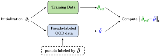
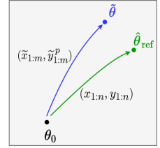
Figure 1: How to compute Projection Norm on unlabeled OOD data. (Left) Given a classifier $\smash{\widehat{\boldsymbol{\theta}}}$, we first pseudo-label the OOD data $\widetilde{\boldsymbol{x}}_{1:m}$ using the predictions of $\smash{\widehat{\boldsymbol{\theta}}}$. Next, we obtain a new network $\smash{\widetilde{\boldsymbol{\theta}}}$ that is initialized with ${\boldsymbol{\theta}}_{0}$ and trained on the pseudo-labeled OOD data. Finally, we train a reference network $\smash{\widehat{\boldsymbol{\theta}}}_{\text{ref}}$ on the training data (with the same initialization ${\boldsymbol{\theta}}_{0}$) and output the $\textsf{ProjNorm}(\mathcal{D}_{\text{train}},\widetilde{\boldsymbol{x}}_{1:m})=\|\smash{\widehat{\boldsymbol{\theta}}}_{\text{ref}}-\smash{\widetilde{\boldsymbol{\theta}}}\|_{2}$. (Right) Schematic of $\smash{\widetilde{\boldsymbol{\theta}}}$ and $\smash{\widehat{\boldsymbol{\theta}}}_{\text{ref}}$ are obtained. See Algorithm 1 for details on computing ProjNorm.

To reliably deploy machine learning models in practice, we must understand the model’s performance on unseen test samples. Conventional machine learning wisdom suggests using a held-out validation set to estimate the model’s test-time performance (Hastie et al., 2001). However, this fails to account for distribution shift. For deep neural networks, even simple distribution shifts can lead to large drops in performance (Quiñonero-Candela et al., 2008; Koh et al., 2021). Thus, it is crucial to understand, especially in safety-critical applications, how a model might perform on out-of-distribution (OOD) data. Finally, understanding OOD performance helps shed light on the structure of natural covariate shifts, which remain poorly understood from a conceptual standpoint (Hendrycks et al., 2021a).

To this end, we propose Projection Norm, which uses unlabeled test samples to help predict the OOD test error. Let $\smash{\widehat{\boldsymbol{\theta}}}$ be the model whose test error we aim to predict. At a high level, the Projection Norm algorithm pseudo-labels the test samples using $\smash{\widehat{\boldsymbol{\theta}}}$ and then uses these pseudo-labels to train a new model $\smash{\widetilde{\boldsymbol{\theta}}}$. Finally, it compares the distance between $\smash{\widehat{\boldsymbol{\theta}}}$ and $\smash{\widetilde{\boldsymbol{\theta}}}$, with a larger distance corresponding to higher test error. We formally present this algorithm in Section 2.

Empirically, we demonstrate that Projection Norm predicts test error more accurately than existing methods (Deng et al., 2021; Guillory et al., 2021; Garg et al., 2022), across several vision and language benchmarks and for different neural network architectures (Section 3.1). Moreover, while the errors of existing methods are highly correlated with each other, the errors of Projection Norm are nearly uncorrelated with those of existing methods (Section 3.3), so combining Projection Norm with these methods results in even better prediction performance. Finally, we stress test our method against adversarial examples, an extreme type of distribution shift, and we find that Projection Norm is the only method that achieves non-trivial performance (Section 5).

Projection Norm also has a natural theoretical motivation. We show for overparameterized linear models that Projection Norm measures the projection (hence the name) of a “ground truth model” onto the overlap of the training and test data (Section 4). In this linear setting, many common methods focus only on the logits and thus cannot capture information that is orthogonal to the training manifold. In contrast, Projection Norm can, which explains why it provides information complementary to that of other methods. We also connect Projection Norm to a mathematical bound on the test loss, based on assumptions backed by empirical studies on vision data (Section 4.3).

In summary, we propose a new metric for predicting OOD error that provides a more accurate and orthogonal signal in comparison to existing approaches. Our method is easy to implement and is applicable to a wide range of prediction tasks. In addition, our method connects naturally to the theory of high-dimensional linear models and attains non-trivial performance even for adversarial examples.

2 Our Method: Projection Norm

In this section, we formulate the problem of predicting OOD performance at test time and then present the Projection Norm algorithm.

Problem formulation. Consider solving a $K$-class classification task using a neural network parameterized by ${\boldsymbol{\theta}}$. Let $f_{1},\dots,f_{K}$ be functions representing the last layer of the neural network and $C({\boldsymbol{x}};{{\boldsymbol{\theta}}})=\arg\max_{i}f_{i}({\boldsymbol{x}};{\boldsymbol{\theta}})$ be the corresponding classifier. Given a training set $\mathcal{D}_{\text{train}}=\{({\boldsymbol{x}}_{i},y_{i})\}_{i=1,\dots,n}$, we use a pre-trained network, denoted by ${\boldsymbol{\theta}}_{0}$, for initialization and fine-tune the network on $\mathcal{D}_{\text{train}}$ by approximately minimizing the training loss (e.g. via SGD). We denote the parameters of the fine-tuned network by $\smash{\widehat{\boldsymbol{\theta}}}$.

At test time, the fine-tuned classifier $C(\cdot;\smash{\widehat{\boldsymbol{\theta}}})$ is then tested on $m$ (out-of-distribution) test samples $\widetilde{\boldsymbol{x}}_{1:m}$ with corresponding unobserved labels $\widetilde{y}_{1:m}$. The test error on OOD data $\widetilde{\boldsymbol{x}}_{1:m}$ is defined as

$$\textsf{TestError}(\widetilde{\boldsymbol{x}}_{1:m},\widetilde{y}_{1:m},\smash{\widehat{\boldsymbol{\theta}}})=\frac{1}{m}\sum_{j=1}^{m}\mathbf{1}\big{\{}C(\widetilde{\boldsymbol{x}}_{j};\smash{\widehat{\boldsymbol{\theta}}})\neq\widetilde{y}_{j}\big{\}}.\vspace{-0.075in}$$

Our goal is to propose a quantity, without access to the test labels $\widetilde{y}_{1:m}$, that correlates well with the test error across different distribution shifts.

2.1 Projection norm

To this end, we introduce the Projection Norm metric, denoted by $\textsf{ProjNorm}(\mathcal{D}_{\text{train}},\widetilde{\boldsymbol{x}}_{1:m})$, which empirically correlates well with the test error. At a high level, our method consists of three steps (illustrated in Figure 1):

• Step 1: Pseudo-label the test set. Given a classifier $C(\cdot;\smash{\widehat{\boldsymbol{\theta}}})$ and test samples $\widetilde{\boldsymbol{x}}_{1:m}$, compute “pseudo-labels” $\widetilde{y}^{\,p}_{j}=C(\widetilde{\boldsymbol{x}}_{j};\smash{\widehat{\boldsymbol{\theta}}})$.

• Step 2: Fine-tune on the pseudo-labels. Initialize a fresh network with pre-trained parameters ${\boldsymbol{\theta}}_{0}$, then fine-tune on the $m$ pseudo-labeled OOD data points to obtain a model $\smash{\widetilde{\boldsymbol{\theta}}}$.

• Step 3: Compute the distance to a reference model. Finally, we define the Projection Norm as the Euclidean distance to a reference model $\smash{\widehat{\boldsymbol{\theta}}}_{\text{ref}}$:

  $$\textsf{ProjNorm}(\mathcal{D}_{\text{train}},\widetilde{\boldsymbol{x}}_{1:m})=\|\smash{\widehat{\boldsymbol{\theta}}}_{\text{ref}}-\smash{\widetilde{\boldsymbol{\theta}}}\|_{2}.$$ (1)

We can take $\smash{\widehat{\boldsymbol{\theta}}}_{\text{ref}}=\smash{\widehat{\boldsymbol{\theta}}}$; however, $\smash{\widehat{\boldsymbol{\theta}}}$ may be trained on many more samples than $\smash{\widetilde{\boldsymbol{\theta}}}$, so an intuitive choice for $\smash{\widehat{\boldsymbol{\theta}}}_{\text{ref}}$ is to instead fine-tune ${\boldsymbol{\theta}}_{0}$ on $m$ samples from the training set, using the same fine-tuning procedure as Step 2. We find that both choices yield similar performance (Section 3.2), and use the latter for our mainline experiments. Fine-tuning $\smash{\widehat{\boldsymbol{\theta}}}_{\text{ref}}$ and $\smash{\widetilde{\boldsymbol{\theta}}}$ requires $m$ to be reasonably large to achieve meaningful results (see Section 3.2).

We will see in Section 4 that Steps 1 and 2 essentially perform a “nonlinear projection” of $\smash{\widehat{\boldsymbol{\theta}}}$ onto the span of OOD samples $\widetilde{\boldsymbol{x}}_{1:m}$, which is where the name Projection Norm came from. Intuitively, $\smash{\widetilde{\boldsymbol{\theta}}}$ has a subset of the information in $\smash{\widehat{\boldsymbol{\theta}}}$ (since it is trained on the latter model’s pseudo-labels). The smaller the overlap between train and test, the less this information will be retained and the further $\smash{\widetilde{\boldsymbol{\theta}}}$ will be from the reference model.

As we will show in Section 4, an advantage of our method is that it captures information orthogonal to the training manifold (in contrast to other methods) and can be connected to a bound on the test error. Before diving into theoretical analysis, we first study the empirical performance of ProjNorm to demonstrate its effectiveness.

Table 1: Summary of prediction performance on CIFAR10, CIFAR100, and MNLI. We compute coefficients of determination ($R^{2}$) and rank correlations ($\rho$) for existing methods and ProjNorm to compare prediction performance (higher is better). The highest $R^{2}$ and $\rho$ quantities in each row are in bold.

Dataset	Network	Rotation		ConfScore		Entropy		AgreeScore		ATC		ProjNorm
		$R^{2}$	$\rho$	$R^{2}$	$\rho$	$R^{2}$	$\rho$	$R^{2}$	$\rho$	$R^{2}$	$\rho$	$R^{2}$	$\rho$
CIFAR10	ResNet18	0.839	0.953	0.847	0.981	0.872	0.983	0.556	0.871	0.860	0.983	0.962	0.992
	ResNet50	0.784	0.950	0.935	0.993	0.946	0.994	0.739	0.961	0.949	0.994	0.951	0.991
	VGG11	0.826	0.876	0.929	0.988	0.927	0.989	0.907	0.989	0.931	0.989	0.891	0.991
	Average	0.816	0.926	0.904	0.987	0.915	0.989	0.734	0.940	0.913	0.989	0.935	0.991
CIFAR100	ResNet18	0.903	0.955	0.917	0.958	0.879	0.938	0.939	0.969	0.934	0.966	0.978	0.989
	ResNet50	0.916	0.963	0.932	0.986	0.905	0.980	0.927	0.985	0.947	0.989	0.984	0.993
	VGG11	0.780	0.945	0.899	0.981	0.880	0.979	0.919	0.988	0.935	0.986	0.953	0.993
	Average	0.866	0.954	0.916	0.975	0.888	0.966	0.928	0.981	0.939	0.980	0.972	0.992
MNLI	BERT	-	-	0.516	0.671	0.533	0.734	0.318	0.524	0.524	0.699	0.585	0.664
	RoBERTa	-	-	0.493	0.727	0.498	0.734	0.499	0.762	0.519	0.734	0.621	0.790
	Average	-	-	0.505	0.699	0.516	0.734	0.409	0.643	0.522	0.717	0.603	0.727

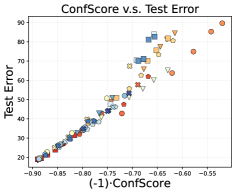
(a) ConfScore

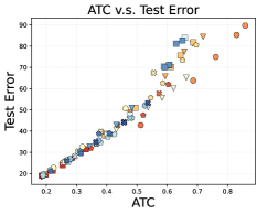
(b) ATC

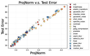
(c) ProjNorm

Figure 2: Generalization prediction versus test error on CIFAR100 with ResNet50. Compare out-of-distribution prediction performance of ConfScore (left), ATC (middle), and ProjNorm (right) on CIFAR100. We plot the actual test error and the method prediction on each OOD dataset. Each point represents one InD/OOD dataset, and points with the same color and marker shape are the same corruption but with different severity levels.

3 Experimental Results

We evaluate the ProjNorm algorithm on several out-of-distribution datasets in the vision and language domains. We first compare our method with existing methods and demonstrate its effectiveness (Section 3.1). Next, we study the sensitivity of ProjNorm to hyperparameters and data set size (Section 3.2). Finally, we show that the errors of ProjNorm are nearly uncorrelated with those of existing methods (Section 3.3), and use this to construct an ensemble method that is even more accurate than ProjNorm alone.

Datasets. We evaluate each method we consider on the image classification tasks CIFAR10, CIFAR100 (Krizhevsky et al., 2009) and the natural language inference task MNLI (Williams et al., 2017). To generate out-of-distribution data, for the CIFAR datasets we use the “common corruptions” of Hendrycks & Dietterich (2019), CIFAR10-C and CIFAR100-C, spanning 18 types of corruption with 5 severity levels. For MNLI, we use BREAK-NLI (Glockner et al., 2018), EQUATE (Ravichander et al., 2019), HANS (McCoy et al., 2019), MNLI-M, MNLI-MM, SICK (Marelli et al., 2014), SNLI (Bowman et al., 2015), STRESS-TEST (Naik et al., 2018), and SICK (Marelli et al., 2014) as out-of-distribution datasets, with STRESS-TEST containing 5 sub-datasets. These OOD datasets include shifts such as swapping words, word overlap, length mismatch, etc. (More comprehensive descriptions of these datasets can be found in Zhou et al. (2020).)

Methods. We consider five existing methods for predicting OOD error: Rotation Prediction (Rotation) (Deng et al., 2021), Averaged Confidence (ConfScore) (Hendrycks & Gimpel, 2016), Entropy (Guillory et al., 2021), Agreement Score (AgreeScore) (Madani et al., 2004; Nakkiran & Bansal, 2020; Jiang et al., 2021), and Averaged Threshold Confidence (ATC) (Garg et al., 2022). Rotation evaluates rotation prediction accuracy on test samples to predict test error. AgreeScore measures agreement rate between two independently trained classifiers on unlabeled test data. ConfScore, Entropy, and ATC predict test error on OOD data based on softmax outputs of the model. See Appendix A.1 for more details of these existing methods.

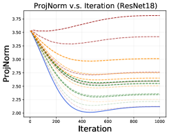
(a) ResNet18.

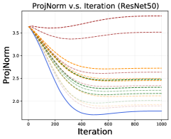
(b) ResNet50.

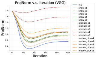
(c) VGG11.

Figure 3: Evaluation of ProjNorm as training progresses on CIFAR100. We visualize how the ProjNorm changes as the number of training iterations increases for (a) ResNet18, (b) ResNet50, and (c) VGG11 on CIFAR100. We show results on three corruptions (snow, pixelate, and motion blur) as well as the in-distribution dataset (InD). For complete results, see Appendix B.

Table 2: Hyperparameter sensitivity of ProjNorm. We vary the number of “pseudo-label projection” training iterations ($T$) and the number of test samples ($m$) of ProjNorm, and evaluate the $R^{2}$ statistic. The performance of ProjNorm is relatively stable, but decreases for sample sizes below $1000$.

Dataset	Training iterations ($m$=1000)				Test samples (set $T$=$m/10$)
	$T$=1000	$T$=500	$T$=200		$m$=5000	$m$=2000	$m$=1000	$m$=500	$m$=100
CIFAR10	0.962	0.985	0.983		0.973	0.977	0.980	0.946	0.784
CIFAR100	0.978	0.980	0.959		0.972	0.942	0.942	0.903	0.466

Pre-trained models and training setup. We use pre-trained models and fine-tune on the in-distribution training dataset. For image classification, we use ResNet18, ResNet50 (He et al., 2016), and VGG11 (Simonyan & Zisserman, 2014), all pre-traineded on ImageNet (Deng et al., 2009). We consider BERT (Devlin et al., 2018) and RoBERTa (Liu et al., 2019) for the natural language inference task, fine-tuned on the MNLI training set. For the CIFAR datasets, we fine-tune using SGD with learning rate $10^{-3}$, momentum $0.9$, and cosine learning rate decay (Loshchilov & Hutter, 2016). For MNLI, we use AdamW (Loshchilov & Hutter, 2017) with learning rate $2\cdot 10^{-5}$ and linear learning rate decay. For computing ProjNorm, we apply the same optimizer as fine-tuning on each dataset. The default number of training iterations for ProjNorm is $1000$. For further details, see Appendix A.

Metrics. To evaluate performance, we compute the correlation between the predictions and the actual test accuracies across the OOD test datasets, using $R^{2}$ and rank correlation (Spearman’s $\rho$). We also present scatter plots to compare different methods qualitatively.

3.1 Main results: comparison of all methods

We summarize results for all methods and datasets in Table 1. We find that ProjNorm achieves better performance than existing methods in most settings. On CIFAR100, ProjNorm achieves an averaged $R^{2}$ of $0.972$, while the second-best method (ATC) only obtains $0.939$. The prediction performance of ProjNorm is also more stable than other methods. For Spearman’s $\rho$ on CIFAR10/100, ATC varies from $0.966$ to $0.994$ and AgreeScore varies from $0.871$ to $0.989$. In contrast, ProjNorm achieves $\rho>0.989$ in all settings.

We also provide scatter plots on CIFAR100 in Figure 2. ProjNorm’s better performance primarily comes from better predicting harder OOD datasets. While all methods do well when the test error is below $40\%$, ConfScore and ATC often underpredict the larger test errors. In contrast, ProjNorm does well even for errors of $90\%$. In Section 4, we argue that this is because ProjNorm better captures directions “orthogonal” to the training set. Scatter plots on other methods/datasets can be found in Appendix B.

3.2 Sensitivity analysis and ablations

We investigate the following four questions for ProjNorm: (1) To improve computational efficiency, can we use fewer training iterations to compute ProjNorm while still achieving similar prediction performance? (2) How many test samples $m$ are needed for ProjNorm to perform well? (3) How important is the choice of reference model? (4) What role do the pseudo-labels play in ProjNorm’s performance?

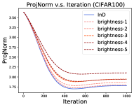
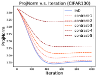
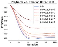
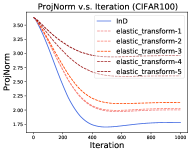
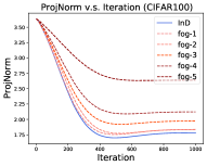
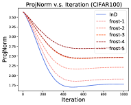
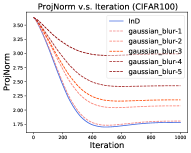
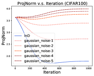
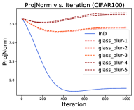
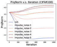
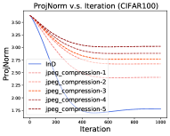
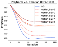
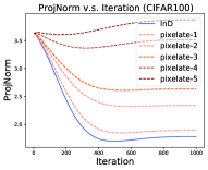
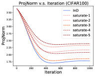
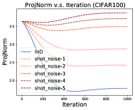
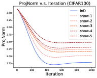
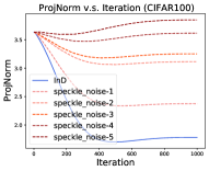
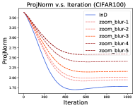
Figure 15: Evaluation of ProjNorm as training progresses on all corruptions in CIFAR100-C. We visualize how the ProjNorm changes as the number of training iteration increases for ResNet50 on CIFAR100.

Training iterations. We first visualize how ProjNorm changes with respect to the number of training iterations. We evaluate ProjNorm at training steps from $1$ to $1000$ and display results for snow, pixelate, and motion blur corruptions in Figure 3 (see Figure 15 for results on all corruptions). For most corruptions in CIFAR10-C and CIFAR100-C, we find that ProjNorm initially decreases with more training iterations, then slowly increases and before converging. Importantly, from Figure 3 we see that the iteration count usually does not affect the ranking of different distribution shifts. Table 2 displays $R^{2}$ values for different iteration counts $T$, and shows that ProjNorm still achieves good performance with as few as $200$ training iterations.

Sample size. We next consider the effect of the number of test samples $m$, varying $m$ from $5000$ to $100$ (from a default size of $10000$). Results are shown in Table 2, where we observe that ProjNorm achieves reasonable performance down to around $1000$ to $2000$ samples, but performs poorly below that. In general, we conjecture that ProjNorm performs well once the number of samples is large enough for fine-tuning to generalize well.

Reference model. We consider directly using $\smash{\widehat{\boldsymbol{\theta}}}$ as the reference model, rather than fine-tuning a new one. As shown in Table 7 and Figure 16 in the appendix, using $\smash{\widehat{\boldsymbol{\theta}}}_{\text{ref}}=\smash{\widehat{\boldsymbol{\theta}}}$ achieves similar performance compared to the default version of ProjNorm on CIFAR10.

Pseudo-labels. Finally, we investigate the role of pseudo-labels in our method. We modify Step 2 of ProjNorm by training $\smash{\widetilde{\boldsymbol{\theta}}}$ using the ground truth labels of the OOD data. From Table 8 and Figure 17, we find that ProjNorm with pseudo-label performs much better than ProjNorm with ground truth label, which suggests that pseudo-labeling is an essential component in ProjNorm.

3.3 Correlation analysis

In this section, we provide a short statistical analysis of using different measurements to predict test error. We focus on the CIFAR100 dataset and Resnet18 architecture. We show that ProjNorm captures signal that existing methods fail to detect, so that ensembling with the existing approaches leads to even better performance.

For each method, we first compute residuals when predicting the test error by performing simple linear regression. Then we compute the correlation between the residual errors for each pair of methods.

Table 3: Correlation of residuals of regressing test error against different measurements with CIFAR100 and ResNet18.

	Ent.	ConfS.	ATC	Rota.	Proj.
Agree.S.	0.85	0.87	0.84	0.80	0.05
Ent.	-	0.98	0.93	0.67	-0.07
ConfS.	-	-	0.98	0.67	-0.14
ATC	-	-	-	0.65	-0.19
Rota.	-	-	-	-	0.03

We see from Table 3 that the correlation among all existing methods is high: strictly larger than $0.6$. The correlations among ConfScore, ATC and Entropy are especially high ($>\!0.9$) suggesting they are almost equivalent approaches. This high correlation is unsurprising since these methods are all different ways of manipulating the logits.

In contrast, the correlation between ProjNorm and existing methods is always less than $0.05$, and often negative. Intriguingly, while the correlations among existing methods are positive, ProjNorm sometimes has negative correlation with existing methods. This means ProjNorm underestimates the test error when other methods overestimate it.

The low correlation implies that ProjNorm provides very different signal compared to existing methods and suggests a natural ensembling approach for improving performance further. Indeed, if we average ProjNorm and ATC (the second best method), normalized by standard deviation, we further improve $R^{2}$ from 0.978 (using ProjNorm only) to 0.982 (averaging ProjNorm and ATC).

4 Insights from an Overparameterized Linear Model

In this section, we provide some insights for Projection Norm by studying its behavior on high-dimensional linear models. We demonstrate an extreme example where Projection Norm has a qualitative advantage over other methods such as Confidence Score. We also show that Projection Norm is tied to an upper bound on the test loss under certain assumptions, which we empirically validate on the CIFAR10 dataset.

We consider a linear model with covariates ${\boldsymbol{x}}\in\mathbb{R}^{d}$ and response $y\in\mathbb{R}$. Let ${\boldsymbol{X}}\in\mathbb{R}^{n\times d}$ and ${\boldsymbol{y}}\in\mathbb{R}^{n}$ denote the training set $\mathcal{D}_{\text{train}}=\{({\boldsymbol{x}}_{i},y_{i})\}_{i=1,\dots,n}$. We focus on the $d\gg n$ regime and take $\smash{\widehat{\boldsymbol{\theta}}}$ to be the minimum-norm interpolating solution,

$$\smash{\widehat{\boldsymbol{\theta}}}=\min_{{\boldsymbol{X}}{\boldsymbol{\theta}}={\boldsymbol{y}}}\|{\boldsymbol{\theta}}\|_{2}={\boldsymbol{X}}^{\mathsf{T}}({\boldsymbol{X}}{\boldsymbol{X}}^{\mathsf{T}})^{-1}{\boldsymbol{y}}.$$ (2)

Let $\widetilde{\boldsymbol{X}}\in\mathbb{R}^{m\times d}$ denote the out-of-distribution test covariates and $\widetilde{\boldsymbol{y}}\in\mathbb{R}^{m}$ the corresponding ground truth response vector. Our goal is to estimate the test loss

$$\textsf{TestLoss}=\frac{1}{m}\|\widetilde{\boldsymbol{X}}\smash{\widehat{\boldsymbol{\theta}}}-\widetilde{\boldsymbol{y}}\|_{2}^{2}$$ (3)

using only ${\boldsymbol{X}}$, ${\boldsymbol{y}}$, and $\widetilde{\boldsymbol{X}}$—that is, without having access to the ground truth response $\widetilde{\boldsymbol{y}}$.

Note that most existing methods in Section 3 (such as the Confidence Score) only look at the outputs of the model $\smash{\widehat{\boldsymbol{\theta}}}$. In this linear setting, this corresponds to the vector $\widetilde{\boldsymbol{X}}\smash{\widehat{\boldsymbol{\theta}}}$. We show (Section 4.1) that any method with this property has severe limitations, while the linear version of Projection Norm overcomes these. Then we present results connecting this linear version of Projection Norm to the test loss (Section 4.2).

4.1 Motivating Projection Norm

To analyze the linear setting, we assume that the responses ${\boldsymbol{y}}$ and $\widetilde{\boldsymbol{y}}$ are noiseless and differ only due to covariate shift:

Assumption 4.1 (Covariate shift).

There exists a ground truth ${\boldsymbol{\theta}}_{\star}\in\mathbb{R}^{d}$ relating the covariates and responses such that ${\boldsymbol{X}}{\boldsymbol{\theta}}_{\star}={\boldsymbol{y}}$ and $\widetilde{\boldsymbol{X}}{\boldsymbol{\theta}}_{\star}=\widetilde{\boldsymbol{y}}$, i.e., for both the in-distribution training data and out-of-distribution test data.

By Assumption 4.1, the minimum-norm solution reduces to

$$\smash{\widehat{\boldsymbol{\theta}}}={\boldsymbol{X}}^{\mathsf{T}}({\boldsymbol{X}}{\boldsymbol{X}}^{\mathsf{T}})^{-1}{\boldsymbol{X}}{\boldsymbol{\theta}}_{\star}={\boldsymbol{P}}{\boldsymbol{\theta}}_{\star},$$ (4)

where ${\boldsymbol{P}}$ is defined as the orthogonal projection matrix onto the row space of ${\boldsymbol{X}}$, i.e., ${\boldsymbol{P}}={\boldsymbol{X}}^{\mathsf{T}}({\boldsymbol{X}}{\boldsymbol{X}}^{\mathsf{T}})^{-1}{\boldsymbol{X}}$. Similarly, let $\widetilde{\boldsymbol{P}}$ be the projection matrix for the row space of $\widetilde{\boldsymbol{X}}$. Using the fact that $\smash{\widehat{\boldsymbol{\theta}}}={\boldsymbol{P}}{\boldsymbol{\theta}}^{*}$ and $\widetilde{\boldsymbol{y}}=\widetilde{\boldsymbol{X}}{\boldsymbol{\theta}}^{*}$, the test loss in (3) can be written as

$$\textsf{TestLoss}=\frac{1}{m}\|\widetilde{\boldsymbol{X}}({\boldsymbol{I}}-{\boldsymbol{P}}){\boldsymbol{\theta}}_{\star}\|_{2}^{2}.$$ (5)

From Eq. (5), we see that the test loss depends on the portion of ${\boldsymbol{\theta}}_{\star}$ that is orthogonal to ${\boldsymbol{X}}$—i.e., in the span of $\widetilde{\boldsymbol{X}}$ but not ${\boldsymbol{X}}$. Now consider any method that depends only on the model output $\widetilde{\boldsymbol{X}}\smash{\widehat{\boldsymbol{\theta}}}=\widetilde{\boldsymbol{X}}{\boldsymbol{P}}{\boldsymbol{\theta}}_{\star}$—such a method is not sensitive to this orthogonal component at all! We can see this concretely through the following setting with Gaussian covariates:

$${\boldsymbol{x}}_{i} \overset{i.i.d.}{\sim}\mathcal{N}\left({\boldsymbol{0}},\left[\begin{array}[]{cc}{\boldsymbol{I}}_{d_{1}}&{\boldsymbol{0}}\\ {\boldsymbol{0}}&{\boldsymbol{0}}\end{array}\right]\right),\;i=1,\ldots,n,$$ (8)

$$\widetilde{\boldsymbol{x}}_{j} \overset{i.i.d.}{\sim}\mathcal{N}\left({\boldsymbol{0}},\left[\begin{array}[]{cc}{\boldsymbol{I}}_{d_{1}}&{\boldsymbol{0}}\\ {\boldsymbol{0}}&\sigma^{2}{\boldsymbol{I}}_{d_{2}}\end{array}\right]\right),\;j=1,\ldots,m.$$ (11)

Here we decompose the $d$-dimensional covariate space into two orthogonal components $d=d_{1}+d_{2}$, where the last $d_{2}$ components appear only at test time. We display empirical results for this distribution in Figure 4 (see Appendix C for full experimental details). Methods that depend only on the model outputs—such as the confidence score—are totally insensitive to the parameter $\sigma$.

Advantage of projection norm. We next define a linear version of the Projection Norm:

$$\textsf{ProjNormLinear}=\|\smash{\widehat{\boldsymbol{\theta}}}-\widetilde{\boldsymbol{P}}\smash{\widehat{\boldsymbol{\theta}}}\|_{2}.\vspace{-0.05in}$$ (12)

This computes the difference between the reference model $\smash{\widehat{\boldsymbol{\theta}}}$ and a projected model $\widetilde{\boldsymbol{P}}\smash{\widehat{\boldsymbol{\theta}}}$. Before justifying ProjNormLinear  as an adaptation of ProjNorm, we first examine its performance on the example introduced above.

In particular, we show that ProjNormLinear  has the right dependence on $\sigma$ whereas ConfScore does not. In ProjNormLinear, the less overlap $\widetilde{\boldsymbol{X}}$ has with ${\boldsymbol{X}}$, the smaller $\widetilde{\boldsymbol{P}}\smash{\widehat{\boldsymbol{\theta}}}$ will be, so the quantity in Eq. (12) does track the orthogonal component of $\widetilde{\boldsymbol{X}}$. Results for ProjNormLinear, also shown in Figure 4, confirm this. In contrast to the confidence score, ProjNormLinear does vary with $\sigma$, better tracking the test error.

We next explain why ProjNormLinear is the linear version of ProjNorm as defined in Eq. (1) (Section 2). To draw the connection, first note that the projection step $\widetilde{\boldsymbol{P}}\smash{\widehat{\boldsymbol{\theta}}}$ is equivalent to finding the minimum $\ell_{2}$-norm solution of

$$\min_{{\boldsymbol{\theta}}}\|\widetilde{\boldsymbol{X}}{\boldsymbol{\theta}}-\widetilde{\boldsymbol{X}}\smash{\widehat{\boldsymbol{\theta}}}\|_{2}^{2}.\vspace{-0.05in}$$ (13)

In the linear setting, the minimum-norm solution can be obtained by initializing at ${\boldsymbol{\theta}}_{0}=\mathbf{0}$ and performing gradient descent to convergence (Wilson et al., 2017; Hastie et al., 2020). If we write $f^{\textsf{Lin}}({\boldsymbol{x}};{\boldsymbol{\theta}})=\langle{\boldsymbol{x}},{\boldsymbol{\theta}}\rangle$, then Eq. (13) can be equivalently written as

$$\min_{{\boldsymbol{\theta}}}\,\sum_{j=1}^{m}\Big{(}f^{\textsf{Lin}}(\widetilde{\boldsymbol{x}}_{j};{\boldsymbol{\theta}})-f^{\textsf{Lin}}(\widetilde{\boldsymbol{x}}_{j};\smash{\widehat{\boldsymbol{\theta}}}\,)\Big{)}^{2}.\vspace{-0.04in}$$ (14)

In other words, it minimizes the squared loss relative to the pseudo-labels $f^{\textsf{Lin}}(\widetilde{\boldsymbol{x}}_{j},{\boldsymbol{\theta}})$. The metric ProjNormLinear is thus the squared difference between the original ($\smash{\widehat{\boldsymbol{\theta}}}$) and pseudo-labeled model ($\smash{\widetilde{\boldsymbol{\theta}}}=\widetilde{\boldsymbol{P}}\smash{\widehat{\boldsymbol{\theta}}}$) in parameter space, akin to the ProjNorm in the non-linear setting. Note that in this linear setting, there is no distinction between $\smash{\widehat{\boldsymbol{\theta}}}_{\text{ref}}$ and $\smash{\widehat{\boldsymbol{\theta}}}$ as in Section 2.

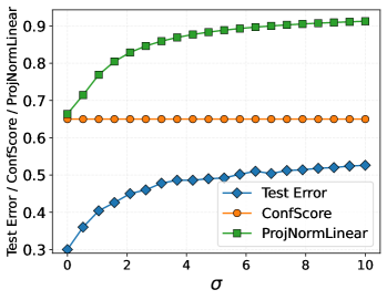
Figure 4: A synthetic binary classification experiment with data distributions defined in Eq. (8) and Eq. (11). The test error increases with $\sigma$, and the linearized version of ProjNorm tracks this, but the confidence score does not.

4.2 Analyzing projection norm

To further explain why ProjNormLinear performs well, we connect it to an upper bound on the test loss, under assumptions that we will empirically investigate in Section 4.3. Our first assumption states that ${\boldsymbol{\theta}}_{\star}$ has the same complexity when projected onto the train and OOD test distributions.

Assumption 4.2 (Projected norm).

We assume that $\|{\boldsymbol{P}}{\boldsymbol{\theta}}_{\star}\|_{2}=\|\widetilde{\boldsymbol{P}}{\boldsymbol{\theta}}_{\star}\|_{2}$.

Our second assumption is on the spectral properties of the covariance matrices:

Assumption 4.3 (Spectral properties).

Write the eigendecomposition of the empirical training and test covariance as

$${\boldsymbol{\Sigma}}=\frac{1}{n}{\boldsymbol{X}}^{\mathsf{T}}{\boldsymbol{X}}=\frac{1}{n}\sum_{i=1}^{n}\mu_{i}{\boldsymbol{u}}_{i}{\boldsymbol{u}}_{i}^{\mathsf{T}},$$ (15)

$$\widetilde{\boldsymbol{\Sigma}}=\frac{1}{m}\widetilde{\boldsymbol{X}}^{\mathsf{T}}\widetilde{\boldsymbol{X}}=\frac{1}{m}\sum_{i=1}^{m}\lambda_{j}{\boldsymbol{v}}_{j}{\boldsymbol{v}}_{j}^{\mathsf{T}},\vspace{-0.05in}$$ (16)

where $\mu_{1}\geq\dots\geq\mu_{n}$ and $\lambda_{1}\geq\dots\geq\lambda_{m}$. We assume there exists some constant $0<k<\min(m,n)$ such that

$$\text{Span}\{{\boldsymbol{u}}_{1},\dots,{\boldsymbol{u}}_{k}\}=\text{Span}\{{\boldsymbol{v}}_{1},\dots,{\boldsymbol{v}}_{k}\}\vspace{-0.075in}$$ (17)

and

$$\text{Span}\{{\boldsymbol{u}}_{k+1},\dots,{\boldsymbol{u}}_{n}\}\,\cap\,\text{Span}\{{\boldsymbol{v}}_{k+1},\dots,{\boldsymbol{v}}_{m}\}=\mathbf{0}.$$ (18)

In other words, we assume the large eigenvectors of the train and OOD test covariates span a common subspace, while the small eigenvectors are orthogonal. Under these assumptions, we show that the TestLoss is bounded by a (constant) multiple of ProjNormLinear.

Proposition 4.4.

Under Assumptions 4.1, 4.2, and 4.3,

$$\frac{\lambda_{m}}{m}\leq\frac{\textsf{TestLoss}}{\textsf{ProjNormLinear}^{~{}2}}\leq\frac{\lambda_{k+1}}{m},$$

where $\lambda_{m},\lambda_{k+1}$ are the $m$-th and $(k+1)$-th eigenvalue of the covariance matrix $\widetilde{\boldsymbol{X}}^{\mathsf{T}}\widetilde{\boldsymbol{X}}/m$.

This offers mathematical intuition for the effectiveness of Projection Norm that we observed in Section 3.

4.3 Checking assumptions on linearized representations

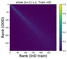
(a) Eigenvector alignment ${\boldsymbol{H}}$.

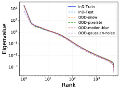
(b) Eigenvalue decay.

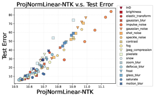
(c) ProjNormLinear-NTK predicts OOD error.

Figure 5: Experimental results on NTKs. (a) We visualize the alignment matrix ${\boldsymbol{H}}\in\mathbb{R}^{300\times 300}$ between top-300 eigenvectors of covariance matrices for in-distribution ($\{{\boldsymbol{u}}_{1},\cdots,{\boldsymbol{u}}_{300}\}$) and OOD (snow) ($\{{\boldsymbol{v}}_{1},\cdots,{\boldsymbol{v}}_{300}\}$) datasets, where ${\boldsymbol{H}}_{ij}=|\langle{\boldsymbol{v}}_{i},{\boldsymbol{u}}_{j}\rangle|$ for $i,j\in[n]$. (b) Eigenvalue decay of kernels on a $\log$-$\log$ scale, including in-distribution train, in-distribution test, snow, pixelate, motion blur, and Gaussian noise with severity 1 from CIFAR10-C. (c) Scatter plot of ProjNormLinear computed on NTK representations versus true test error of model fine-tuned with SGD on CIFAR10-C ($R^{2}=0.914$; $\rho=0.960$). See Appendix D for more results on different corruptions/severities on CIFAR10-C.

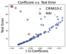
(a) ConfScore.

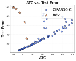
(b) ATC.

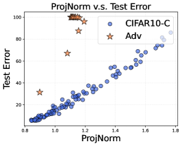
(c) ProjNorm.

Figure 6: Evaluation of ConfScore, ATC, and ProjNorm on predicting OOD error under adversarial attack. Blue circles are results evaluated on CIFAR10-C (each point corresponds to one corrupted test dataset), and orange stars are results evaluated on adversarial examples (each point corresponds to one perturbation radius $\varepsilon$).

In this subsection, we check Assumptions 4.2 and 4.3 on linear representations derived from the CIFAR datasets. To construct the linear representation, consider an image input ${\boldsymbol{x}}_{\text{img}}$ and a neural network $f(\,\cdot\,;{\boldsymbol{\theta}})$. The behavior of the network can be locally approximated by its linearized counterpart (Jacot et al., 2018; Lee et al., 2019), i.e.,

$$f({\boldsymbol{x}}_{\text{img}};{\boldsymbol{\theta}})\approx f({\boldsymbol{x}}_{\text{img}};{\boldsymbol{\theta}}_{\text{0}})+\langle\nabla_{\boldsymbol{\theta}}f({\boldsymbol{x}}_{\text{img}};{\boldsymbol{\theta}}_{\text{0}}),{\boldsymbol{\theta}}-{\boldsymbol{\theta}}_{\text{0}}\rangle.$$

Under this approximation, we can replace the neural network training on the raw data ${\boldsymbol{x}}_{\text{img}}$ by linear regression on its Neural Tangent Kernel (NTK) representation ${\boldsymbol{x}}_{\text{ntk}}$:

$${\boldsymbol{x}}_{\text{ntk}}=\nabla_{\boldsymbol{\theta}}f({\boldsymbol{x}}_{\text{img}};{\boldsymbol{\theta}}_{0})\in\mathbb{R}^{d}.\vspace{-0.01in}$$ (19)

We therefore test the assumptions from Section 4.2 on these NTK representations.

In the most of our experiments, we derive NTK representations from a pretrained ResNet18, which has dimension $d=500,000$ (we randomly subsample 500,000 parameters from a total of 11,177,025 parameters). See Appendix D for more details.

Justification of Assumption 4.2 and 4.3. We first compute the NTK representations of the training data and OOD data on CIFAR10 with sample size $n=m=5,000$. Then we evaluate $\|\widetilde{\boldsymbol{P}}{\boldsymbol{\theta}}_{\star}\|_{2}$ on each OOD datasets in CIFAR10-C and compare with $\|{\boldsymbol{P}}{\boldsymbol{\theta}}_{\star}\|_{2}$. As shown in Figure 19, $\|\widetilde{\boldsymbol{P}}{\boldsymbol{\theta}}_{\star}\|_{2}$ and $\|{\boldsymbol{P}}{\boldsymbol{\theta}}_{\star}\|_{2}$ are within a multiplicative factor of $2$ on most of the OOD datasets.

Next, we compute the eigenvalues and top-$K$ ($K=300$) eigenvectors of ${\boldsymbol{\Sigma}}_{\text{ntk}}={\boldsymbol{X}}_{\text{ntk}}^{\mathsf{T}}{\boldsymbol{X}}_{\text{ntk}}/n$ and $\widetilde{\boldsymbol{\Sigma}}_{\text{ntk}}=\widetilde{\boldsymbol{X}}_{\text{ntk}}^{\mathsf{T}}\widetilde{\boldsymbol{X}}_{\text{ntk}}/m$. As shown in Figure 5(a), the top-$k$ ($k\leq 200$) eigenvectors of in-distribution and OOD covariance matrices align well with each other. When $k$ is large, the in-distribution and OOD eigenvectors become more orthogonal to each other. This suggests that our assumptions on covariance matrices (i.e., Assumption 4.3) approximately align with real data.

We also visualize the eigenvalues of ${\boldsymbol{\Sigma}}_{\text{ntk}}$ and $\widetilde{\boldsymbol{\Sigma}}_{\text{ntk}}$ in Figure 5(b). We find that the eigenvalues of both the in-distribution and OOD covariance matrices approximately follow power-law scaling relations with respect to the index of the eigenvalue.

Linear representations predict nonlinear OOD error. To check that our linear analysis actually captures nonlinear neural network behavior, we use ProjNormLinear on the NTK representation to predict the error of the original, nonlinear neural network (i.e. fine-tuned Resnet18 on CIFAR10). We display the results in Figure 5(c). We find that ProjNormLinear computed on NTK representations predicts the OOD error of its nonlinear counterpart trained by SGD ($R^{2}=0.914$). Compared to results in the first row of Table 1, ProjNormLinear is less accurate than ProjNorm ($R^{2}=0.962$), but still more accurate than all existing methods in terms of $R^{2}$.

5 Stress Test: Adversarial Examples

Finally, we construct a “stress test” to explore the limits of our method. We test our method against adversarial examples, optimized to fool the network into misclassifying, but not specifically optimized to evade detection.

In more detail, we consider white-box $\ell_{\infty}$ attacks on the CIFAR10 dataset, with adversarial perturbation budget $\varepsilon$ ranging from $0.25$ to $8.0$. We generate attacks using $20$ steps of projected gradient descent (PGD), using the untargeted attack of Kurakin et al. (2017). The adversarial OOD test distribution is obtained by computing an adversarial example from each image in the CIFAR10 test set.

We present scatter plots of the performances of ProjNorm, ATC, and ConfScore in Figure 6. For large adversarial perturbation budgets, ATC and ConfScore perform trivially (assigning a minimal score even though the test error is maximal). While ProjNorm also struggles, underpredicting the test error significantly, it stands apart by making non-trivial predictions even for large budgets.

To quantify this numerically, we convert each method to an OOD error estimate by calibrating on CIFAR10-C (i.e. running linear regression on the blue circles in Figure 6). For $\varepsilon=8$, ProjNorm predicts an error of $28.1\%$ when the true error is $100.0\%$, whereas predictions of other methods are smaller than $0.0\%$. Full results for all methods are in Table 10.

Such a stress test could be an interesting target for future work. While detecting adversarial examples is notoriously difficult (Carlini & Wagner, 2017), this setting may be more tractable because an entire distribution of data points is observed, rather than a single point.

6 Related Work

Predicting OOD generalization. Predicting OOD error from test samples is also called unsupervised risk estimation (Donmez et al., 2010). Balasubramanian et al. (2011) address this task using Gaussian mixture models, and Steinhardt & Liang (2016) use conditional independence assumptions and the method of moments. In a different direction, Chuang et al. (2020) propose using domain-invariant representations (Ben-David et al., 2007) to estimate model generalization. Deng & Zheng (2021) and Deng et al. (2021) apply rotation prediction to estimate classifier accuracy on vision tasks. Other works propose using the model’s (softmax) predictions on the OOD data (Guillory et al., 2021; Jiang et al., 2021; Garg et al., 2022). Chen et al. (2021) propose an importance weighting approach that leverages prior knowledge.

Robustness. Recent works develop benchmarks for evaluating model performance under various distribution shifts, including vision and language benchmarks (Geirhos et al., 2018; Recht et al., 2019; Hendrycks & Dietterich, 2019; Shankar et al., 2021; Hendrycks et al., 2021b; Santurkar et al., 2021; Hendrycks et al., 2021a; Naik et al., 2018; McCoy et al., 2019; Miller et al., 2020; Koh et al., 2021). Several recent works (Taori et al., 2020; Allen-Zhu et al., 2019) identify the “accuracy on the line” phenomenon—a linear trend between in-distribution accuracy and OOD accuracy. Taori et al. (2020) and Hendrycks et al. (2021a) find that using larger models pre-trained on more (diverse) datasets are two effective techniques for improving robustness. Sun et al. (2020) propose a test-time-training method to improve robustness.

OOD detection. The goal of OOD detection is to identify whether a test sample comes from a different distribution than the training data, which is closely related to the task we study. Hendrycks & Gimpel (2016) and Geifman & El-Yaniv (2017) use model softmax outputs to detect OOD samples. Lee et al. (2018) propose to use a generative classifier for OOD detection. Liang et al. (2018) find that temperature scaling (Guo et al., 2017) and adversarial perturbations (Goodfellow et al., 2014) can improve detection performance. Other work utilizes pre-trained models to improve OOD detection performance (Hendrycks et al., 2020; Xu et al., 2021). Our method can potentially be extended to perform OOD detection.

Domain adaptation. A large body of work studies how to learn representations that transfer from a source domain to a target domain during training (Ben-David et al., 2007, 2010; Pan et al., 2010; Long et al., 2015; Ganin et al., 2016; Tzeng et al., 2017; Zhao et al., 2019). The goal of domain adaptation is to improve model performance on a target (OOD) domain, whereas we focus on predicting performance of a fixed model on OOD data. An interesting direction for future work would be to explore the application of ProjNorm in domain adaptation.

NTK and overparameterized linear models. A recent line of theoretical work tries to connect deep neural network training to neural tangent kernels (NTK) (Jacot et al., 2018; Lee et al., 2019; Du et al., 2019; Allen-Zhu et al., 2019; Zou et al., 2019), showing that infinite-width networks converge to a limiting kernel. Several recent works study the benign overfitting phenomenon in deep learning through overparameterized linear models (Bartlett et al., 2020; Tsigler & Bartlett, 2020; Koehler et al., 2021). Tripuraneni et al. (2021) computes the exact asymptotics of generalization error for random feature models under certain assumptions of distribution shift.

7 Discussion

Thus far, we have focused on the advantages of Projection Norm in terms of empirical performance and theoretical interpretability. We now briefly discuss limitations of Projection Norm and future directions. One limitation is that it needs sufficiently many samples (because of the fine-tuning step) to make accurate predictions on the OOD test dataset. It would be useful to reduce the sample complexity of this method, with the ideal being a one-sample version of ProjNorm. Another issue is that ProjNorm sometimes does poorly on “easy” shifts, as it looks for all differences between two distributions, including those that might make the problem easier. We illustrate this in Figure 18 of the appendix, where ProjNorm typically overpredicts the error under label shifts. A final limitation is ProjNorm’s performance on adversarial examples, which suggests an interesting avenue for future work.

Beyond predicting OOD error, ProjNorm provides a general way to compute distances between distributions. For instance, it could be used to choose sample policies for active learning or exploration policies for reinforcement learning. We see ProjNorm as a particularly promising approach for addressing “novelty” in high-dimensional settings.

Acknowledgements

We would like to thank Aditi Raghunathan, Yu Sun, and Chong You for their valuable feedback and comments. We would also like to thank Keyang Xu and Xiang Zhou for helpful discussions on the NLI experiments.

Appendix A Experimental Details

Details on ProjNorm. Algorithm 1 provides a detailed description of the ProjNorm algorithm.

Algorithm 1 ProjNorm

1:  Input: Classifier $C(\cdot;\smash{\widehat{\boldsymbol{\theta}}})$ to be evaluated, initialization ${\boldsymbol{\theta}}_{0}$, training data $\mathcal{D}_{\text{train}}=\{({\boldsymbol{x}}_{i},y_{i})\}_{i=1}^{n}$, OOD unlabeled test data $\widetilde{\boldsymbol{x}}_{1:m}=\{\widetilde{\boldsymbol{x}}_{j}\}_{j=1}^{m}$.

2:  Parameters: Number of training steps $T$, initial learning rate $\eta$.

3:  Step 1: Pseudo-label OOD data with $C(\cdot;\smash{\widehat{\boldsymbol{\theta}}})$, i.e., $\widetilde{y}^{\,p}_{j}=C(\widetilde{\boldsymbol{x}}_{j};\smash{\widehat{\boldsymbol{\theta}}})$, $j\in[m]$.

4:  Step 2: From initialization ${\boldsymbol{\theta}}_{0}$, train a new model $\smash{\widetilde{\boldsymbol{\theta}}}$ on pseudo-labeled OOD data $\{(\widetilde{\boldsymbol{x}}_{j},\widetilde{y}^{\,p}_{j})\}_{j=1}^{m}$ by performing $T$ steps of stochastic gradient descent updates with learning rate $\eta$.

5:  Step 2+: From initialization ${\boldsymbol{\theta}}_{0}$, train a reference model $\smash{\widehat{\boldsymbol{\theta}}}_{\textsf{ref}}$ on training data $\{({\boldsymbol{x}}_{i},y_{i})\}_{i=1}^{n}$ by performing $T$ steps of stochastic gradient descent updates with learning rate $\eta$.

6:  Step 3: Output $\textsf{ProjNorm}(\mathcal{D}_{\text{train}},\widetilde{\boldsymbol{x}}_{1:m}):=\|\smash{\widehat{\boldsymbol{\theta}}}_{\text{ref}}-\smash{\widetilde{\boldsymbol{\theta}}}\|_{2}.$

Additional implementation details. For the CIFAR datasets, we fine-tune the pre-trained model on in-distribution training data for 20 and 50 epochs for CIFAR10 and CIFAR100, respectively. For MNLI, we fine-tune the pre-trained model for 4 epochs on in-distribution training data.

A.1 Details of existing methods

Rotation. The Rotation Prediction (Rotation) (Deng et al., 2021) metric is defined as

$$\text{Rotation}=\frac{1}{m}\sum_{j=1}^{m}\left\{\frac{1}{4}\sum_{r\in\{0^{\circ},90^{\circ},180^{\circ},270^{\circ}\}}\mathbf{1}\left\{C^{r}(\widetilde{\boldsymbol{x}}_{j};\smash{\widehat{\boldsymbol{\theta}}})\neq y_{r}\right\}\right\},$$ (20)

where $y_{r}$ is the label for $r\in\{0^{\circ},90^{\circ},180^{\circ},270^{\circ}\}$, and $C^{r}(\widetilde{\boldsymbol{x}}_{j};\smash{\widehat{\boldsymbol{\theta}}})$ predicts the rotation degree of an image $\widetilde{\boldsymbol{x}}_{j}$.

ConfScore. The Averaged Confidence (ConfScore) is defined as

$$\text{ConfScore}=\frac{1}{m}\sum_{j=1}^{m}\max_{k}\text{Softmax}(f(\widetilde{\boldsymbol{x}}_{j};\smash{\widehat{\boldsymbol{\theta}}}))_{k},$$ (21)

where $\text{Softmax}(\cdot)$ is the softmax function.

Entropy. The Entropy metric is defined as

$$\text{Entropy}=\frac{1}{m}\sum_{j=1}^{m}\text{Ent}\left(\text{Softmax}(f(\widetilde{\boldsymbol{x}}_{j};\smash{\widehat{\boldsymbol{\theta}}}))\right),$$ (22)

where $\text{Ent}(\boldsymbol{p})=-\sum_{k=1}^{K}\boldsymbol{p}_{k}\cdot\log(\boldsymbol{p}_{k})$.

AgreeScore. The Agreement Score (AgreeScore) is defined as

$$\text{AgreeScore}=\frac{1}{m}\sum_{j=1}^{m}\mathbf{1}\left\{C(\widetilde{\boldsymbol{x}}_{j};{\boldsymbol{\theta}}_{1})\neq C(\widetilde{\boldsymbol{x}}_{j};{\boldsymbol{\theta}}_{2})\right\},$$ (23)

where $C(\widetilde{\boldsymbol{x}}_{j};{\boldsymbol{\theta}}_{1})$ and $C(\widetilde{\boldsymbol{x}}_{j};{\boldsymbol{\theta}}_{2})$ are two classifiers that are trained on in-distribution training data independently.

ATC. The Averaged Threshold Confidence (ATC) (Garg et al., 2022) is defined as

$$\text{ATC}=\frac{1}{m}\sum_{j=1}^{m}\mathbf{1}\left\{s(\text{Softmax}(f(\widetilde{\boldsymbol{x}}_{j};\smash{\widehat{\boldsymbol{\theta}}})))<t\right\},$$ (24)

where $s(\boldsymbol{p})=\sum_{j=1}^{K}\boldsymbol{p}_{k}\log(\boldsymbol{p}_{k})$, and $t$ is defined as the solution to the following equation,

$$\frac{1}{m^{\text{val}}}\sum_{\ell=1}^{m^{\text{val}}}\mathbf{1}\left\{s(\text{Softmax}(f({{\boldsymbol{x}}}^{\text{val}}_{\ell};\smash{\widehat{\boldsymbol{\theta}}})))<t\right\}=\frac{1}{m^{\text{val}}}\sum_{\ell=1}^{m^{\text{val}}}\mathbf{1}\left\{C({{\boldsymbol{x}}}^{\text{val}}_{\ell};\smash{\widehat{\boldsymbol{\theta}}})\neq y^{\text{val}}_{\ell}\right\},$$ (25)

where $({{\boldsymbol{x}}}^{\text{val}}_{\ell},y^{\text{val}}_{\ell})$, $\ell=1,\dots,m^{\text{val}}$, are in-distribution validation samples.

Appendix B Additional Experimental Results

Scatter plots of generalization prediction versus test error. We present the scatter plots for all methods (displayed in Table 1) in Figures 7–14. More specifically, the figures plot results for the following models and datasets:

• CIFAR10: ResNet18 (Figure 7), ResNet50 (Figure 8), and VGG11 (Figure 9).

• CIFAR100: ResNet18 (Figure 10), ResNet50 (Figure 11), VGG11 (Figure 12).

• MNLI: BERT (Figure 13), RoBERTa (Figure 14).

Sensitivity analysis. We present more results on the sensitivity analysis of ProjNorm. We vary the number of iterations $T$ (Table 4), the number of test samples $m$ (Table 5), and the learning rate $\eta$ (Table 6).

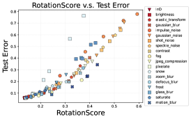
(a) Rotation.

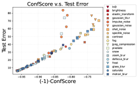
(b) ConfScore.

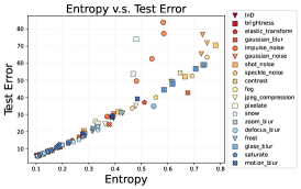
(c) Entropy.

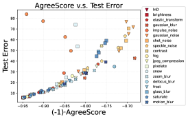
(d) AgreeScore.

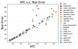
(e) ATC.

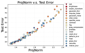
(f) ProjNorm.

Figure 7: Generalization prediction versus test error on CIFAR10 with ResNet18. Compare out-of-distribution prediction performance of all methods. We plot the actual test error and the method prediction on each OOD dataset. Each point represents one InD/OOD dataset, and points with the same color and marker shape are the same corruption but with different severity levels.

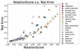
(a) Rotation.

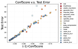
(b) ConfScore.

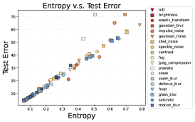
(c) Entropy.

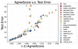
(d) AgreeScore.

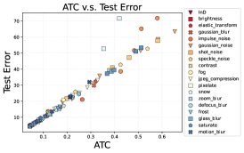
(e) ATC.

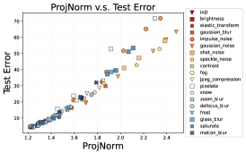
(f) ProjNorm.

Figure 8: Generalization prediction versus test error on CIFAR10 with ResNet50. Compare out-of-distribution prediction performance of all methods. We plot the actual test error and the method prediction on each OOD dataset. Each point represents one InD/OOD dataset, and points with the same color and marker shape are the same corruption but with different severity levels.

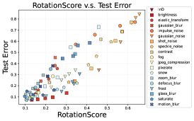
(a) Rotation.

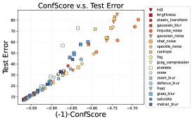
(b) ConfScore.

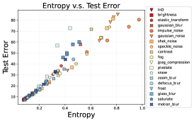
(c) Entropy.

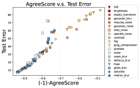
(d) AgreeScore.

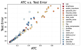
(e) ATC.

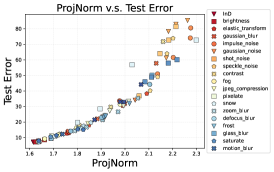
(f) ProjNorm.

Figure 9: Generalization prediction versus test error on CIFAR10 with VGG11. Compare out-of-distribution prediction performance of all methods. We plot the actual test error and the method prediction on each OOD dataset. Each point represents one InD/OOD dataset, and points with the same color and marker shape are the same corruption but with different severity levels.

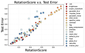
(a) Rotation.

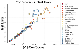
(b) ConfScore.

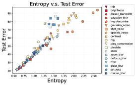
(c) Entropy.

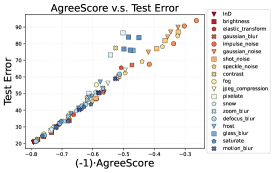
(d) AgreeScore.

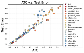
(e) ATC.

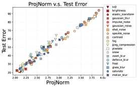
(f) ProjNorm.

Figure 10: Generalization prediction versus test error on CIFAR100 with ResNet18. Compare out-of-distribution prediction performance of all methods. We plot the actual test error and the method prediction on each OOD dataset. Each point represents one InD/OOD dataset, and points with the same color and marker shape are the same corruption but with different severity levels.

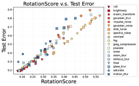
(a) Rotation.

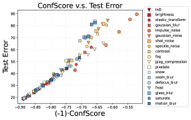
(b) ConfScore.

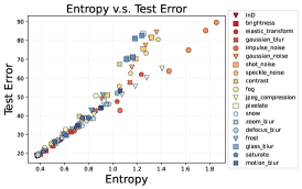
(c) Entropy.

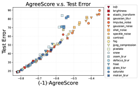
(d) AgreeScore.

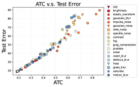
(e) ATC.

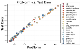
(f) ProjNorm.

Figure 11: Generalization prediction versus test error on CIFAR100 with ResNet50. Compare out-of-distribution prediction performance of all methods. We plot the actual test error and the method prediction on each OOD dataset. Each point represents one InD/OOD dataset, and points with the same color and marker shape are the same corruption but with different severity levels.

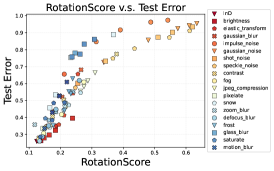
(a) Rotation.

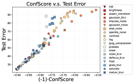
(b) ConfScore.

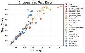
(c) Entropy.

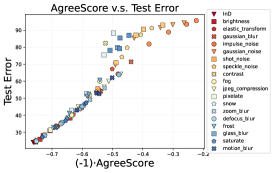
(d) AgreeScore.

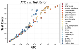
(e) ATC.

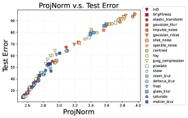
(f) ProjNorm.

Figure 12: Generalization prediction versus test error on CIFAR100 with VGG11. Compare out-of-distribution prediction performance of all methods. We plot the actual test error and the method prediction on each OOD dataset. Each point represents one InD/OOD dataset, and points with the same color and marker shape are the same corruption but with different severity levels.

(a) ConfScore.

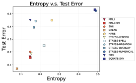
(b) Entropy.

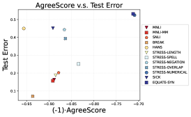
(c) AgreeScore.

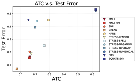
(d) ATC.

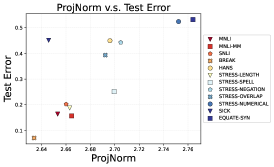
(e) ProjNorm.

Figure 13: Generalization prediction versus test error on MNLI with BERT. Compare out-of-distribution prediction performance of all methods (except for Rotation). We plot the actual test error and the method prediction on each InD/OOD dataset.

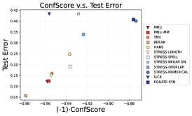
(a) ConfScore.

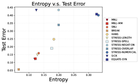
(b) Entropy.

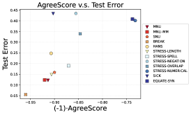
(c) AgreeScore.

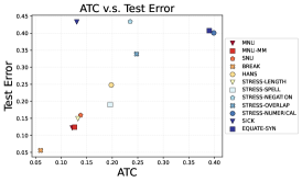
(d) ATC.

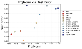
(e) ProjNorm.

Figure 14: Generalization prediction versus test error on MNLI with RoBERTa. Compare out-of-distribution prediction performance of all methods (except for Rotation). We plot the actual test error and the method prediction on each InD/OOD dataset.

Table 4: Hyperparameter sensitivity of ProjNorm (w.r.t. sample size $T$). We vary the number of “pseudo-label projection” training iterations ($T$). We set the number of test samples $m=10,000$. The performance of ProjNorm is stable across different number of training iterations.

Dataset	$T$=1,000		$T$=500		$T$=200
	$R^{2}$	$\rho$	$R^{2}$	$\rho$	$R^{2}$	$\rho$
CIFAR10	0.962	0.992	0.985	0.987	0.983	0.986
CIFAR100	0.978	0.989	0.980	0.986	0.959	0.968

Table 5: Hyperparameter sensitivity of ProjNorm (w.r.t. sample size $m$). We vary the number of test samples ($m$) of ProjNorm. We set learning rate $\eta$=0.001 and number of training iterations $T$=$m/10$.

Dataset	$m=10,000$		$m=5,000$		$m=2,000$		$m=1,000$		$m=500$		$m=100$
	$R^{2}$	$\rho$	$R^{2}$	$\rho$	$R^{2}$	$\rho$	$R^{2}$	$\rho$	$R^{2}$	$\rho$	$R^{2}$	$\rho$
CIFAR10	0.962	0.992	0.973	0.989	0.977	0.985	0.980	0.975	0.946	0.983	0.784	0.896
CIFAR100	0.978	0.989	0.972	0.983	0.942	0.966	0.942	0.981	0.903	0.972	0.466	0.789

Table 6: Hyperparameter sensitivity of ProjNorm (w.r.t. learning rate $\eta$). We vary the learning rate ($\eta$) and set $T$=1,000 and $m$=10,000. The performance of ProjNorm is stable across different learning rates.

Dataset	$\eta$=1e-3		$\eta$=5e-4		$\eta$=1e-4
	$R^{2}$	$\rho$	$R^{2}$	$\rho$	$R^{2}$	$\rho$
CIFAR10	0.962	0.992	0.984	0.991	0.986	0.988
CIFAR100	0.978	0.989	0.982	0.989	0.969	0.984

Comparing $\|\smash{\widetilde{\boldsymbol{\theta}}}-\smash{\widehat{\boldsymbol{\theta}}}\|_{2}$ and $\|\smash{\widetilde{\boldsymbol{\theta}}}-\smash{\widehat{\boldsymbol{\theta}}}_{\text{ref}}\|_{2}$.

We study the performance of ProjNorm when we use $\smash{\widehat{\boldsymbol{\theta}}}$ as $\smash{\widehat{\boldsymbol{\theta}}}_{\text{ref}}$ on CIFAR10. We do not train a new reference model on the training dataset and use the fine-tuned model $\smash{\widehat{\boldsymbol{\theta}}}$ to measure the difference $\|\smash{\widetilde{\boldsymbol{\theta}}}-\smash{\widehat{\boldsymbol{\theta}}}\|_{2}$. As shown in Figure 16, applying $\smash{\widehat{\boldsymbol{\theta}}}_{\text{ref}}=\smash{\widehat{\boldsymbol{\theta}}}$ does not degrade the performance of ProjNorm.

Table 7: Comparing ProjNorm with different reference models on CIFAR10. We study the performance of ProjNorm when using $\smash{\widehat{\boldsymbol{\theta}}}_{\text{ref}}=\smash{\widehat{\boldsymbol{\theta}}}$ and compare it with the default version of ProjNorm. ProjNorm with $\smash{\widehat{\boldsymbol{\theta}}}_{\text{ref}}=\smash{\widehat{\boldsymbol{\theta}}}$ achieves similar or even better performance compared to the default version. We set $T=500$ and $\eta=0.001$.

Dataset	ResNet18		ResNet50		VGG11
	$R^{2}$	$\rho$	$R^{2}$	$\rho$	$R^{2}$	$\rho$
Default	0.980	0.989	0.972	0.986	0.982	0.993
$\smash{\widehat{\boldsymbol{\theta}}}_{\text{ref}}=\smash{\widehat{\boldsymbol{\theta}}}$	0.989	0.991	0.980	0.987	0.982	0.994

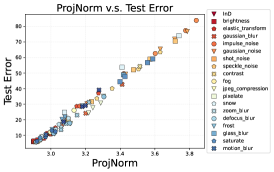
(a) ResNet18.

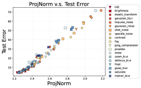
(b) ResNet50.

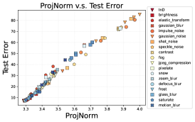
(c) VGG11.

Figure 16: Generalization prediction versus test error on CIFAR10 with ResNet18/ResNet50/VGG11. We plot the actual test error and the prediction of ProjNorm (when $\smash{\widehat{\boldsymbol{\theta}}}_{\text{ref}}=\smash{\widehat{\boldsymbol{\theta}}}$) on each OOD dataset. Each point represents one InD/OOD dataset, and points with the same color and marker shape are the same corruption but with different severity levels.

Role of pseudo-labels.

We investigate the role of pseudo-labels in ProjNorm. Specifically, we modify Step 2 of ProjNorm by training $\smash{\widetilde{\boldsymbol{\theta}}}$ using the ground truth labels of the OOD data. We compare the performance of ProjNorm when using pseudo-labels and ground truth labels. As shown in Figure 17, we find that ProjNorm with pseudo-label performs much better than ProjNorm with ground truth label, which suggests that pseudo-labeling is an essential component of ProjNorm.

Table 8: Comparing ProjNorm with pseudo-labels and ground truth labels on CIFAR10. We study the performance of ProjNorm when using ground truth labels of OOD data (in Step 2) and compare it with the default version of ProjNorm. ProjNorm with ground truth labels achieves worse performance compared to the default version. We set $T=500$ and $\eta=0.001$.

Dataset	ResNet18		ResNet50		VGG11
	$R^{2}$	$\rho$	$R^{2}$	$\rho$	$R^{2}$	$\rho$
Default	0.980	0.989	0.972	0.986	0.982	0.993
Ground truth labels	0.833	0.952	0.813	0.946	0.870	0.961

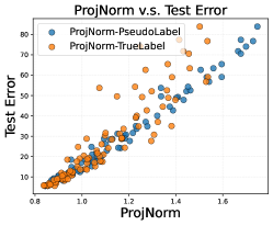
(a) ResNet18.

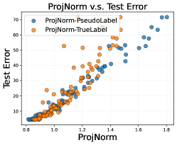
(b) ResNet50.

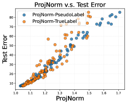
(c) VGG11.

Figure 17: Comparing the performance of ProjNorm when using pseudo-labels and ground truth labels on CIFAR10. We plot the actual test error and the prediction of ProjNorm on each OOD dataset. Blue circles are results when using pseudo-labels, and orange circles are results when using ground truth labels.

Evaluation on label shift.

We evaluate our method and existing methods on CIFAR100 under label shift. Specifically, we measure the test error of each class from the in-distribution test dataset. Then, we rank the classes by the test error of each class (in descending order), i.e., $(c_{1}^{r},c_{2}^{r},\dots,c_{100}^{r})$. Finally, we partition the test dataset into five datasets $(D_{1},\dots,D_{5})$, where $D_{j}$ contains classes $((j-1)\cdot 20+1,\dots,j\cdot 20))$. The results are summarized in Figure 18. We find that ProjNorm performs worse than existing methods.

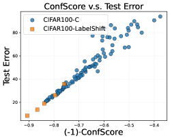
(a) ConfScore.

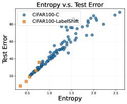
(b) Entropy.

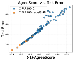
(c) AgreeScore.

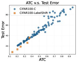
(d) ATC.

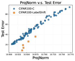
(e) ProjNorm.

Figure 18: Generalization prediction versus test error on CIFAR100 with ResNet18. Compare out-of-distribution prediction performance of all methods. We plot the actual test error and the method prediction on each InD/OOD dataset. Blue circles are results evaluated on CIFAR100-C, and orange squares are results evaluated on 5 test datasets under label shift.

Appendix C Details for the Toy Experiments

We construct a synthetic classification task with ${\boldsymbol{x}}\in\mathbb{R}^{d}$ with

$$\text{Training coviarte distribution:~{}}\mathcal{N}\left({\boldsymbol{0}},\left[\begin{array}[]{cc}{\boldsymbol{I}}_{d_{1}}&{\boldsymbol{0}}\\ {\boldsymbol{0}}&{\boldsymbol{0}}\end{array}\right]\right).$$

$$\text{Test coviarte distribution:~{}}\mathcal{N}\left({\boldsymbol{0}},\left[\begin{array}[]{cc}{\boldsymbol{I}}_{d_{1}}&{\boldsymbol{0}}\\ {\boldsymbol{0}}&\sigma^{2}{\boldsymbol{I}}_{d_{2}}\end{array}\right]\right).$$

We set $d_{1}=1000$ and $d_{2}=500$. For both the training and test distributions, we assume class membership is given by

$$y|{\boldsymbol{x}}=\text{sign}({\boldsymbol{x}}[1]+{\boldsymbol{x}}[1500]).$$

Given the definition of the training and test distributions, we sample $n=500$ training samples and $m=500$ test samples. Then, we perform the two-class linear regression to obtain Figure 4.

Appendix D Details for NTK Experiments

As shown in Figure 19, we visualize the evaluations of $(\|\widetilde{\boldsymbol{P}}{\boldsymbol{\theta}}_{\star}\|-\|{\boldsymbol{P}}{\boldsymbol{\theta}}_{\star}\|)/\|{\boldsymbol{P}}{\boldsymbol{\theta}}_{\star}\|$ for all corruptions in CIFAR10-C. We present the eigenvalue decay results in Figure 20, which include all corruptions in CIFAR10-C.

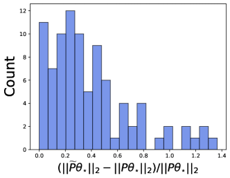
Figure 19: Evaluation of $(\|\widetilde{\boldsymbol{P}}{\boldsymbol{\theta}}_{\star}\|-\|{\boldsymbol{P}}{\boldsymbol{\theta}}_{\star}\|)/\|{\boldsymbol{P}}{\boldsymbol{\theta}}_{\star}\|$ on all OOD datasets from CIFAR10-C. We empirically study Assumption 4.2 on CIFAR10-C. For each dataset in CIFAR10-C, we first randomly subsample 5,000 data points, $(\widetilde{\boldsymbol{X}}_{\text{input}},\widetilde{\boldsymbol{y}})$. Then we use the ImageNet pre-trained ResNet18 to obtain NTK representations of the OOD data, i.e., $\widetilde{\boldsymbol{X}}$. Then we set $\widetilde{\boldsymbol{P}}{\boldsymbol{\theta}}_{\star}=\text{argmin}_{{\boldsymbol{\theta}}}\|\widetilde{\boldsymbol{X}}{\boldsymbol{\theta}}-\widetilde{\boldsymbol{y}}\|_{2}^{2}$, and measure $\|\widetilde{\boldsymbol{P}}{\boldsymbol{\theta}}_{\star}\|$.

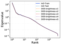
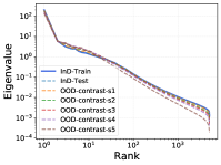
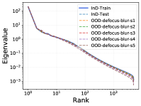
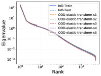
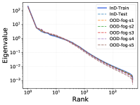
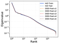
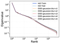
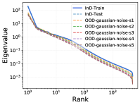
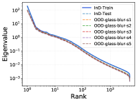
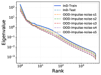
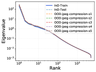
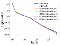
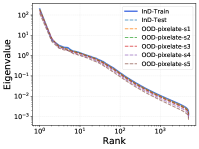
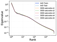
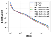
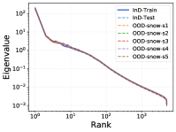
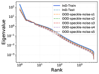
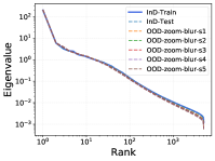
Figure 20: Results on eigenvalue decay in $\log$-$\log$ scale, including InD train, InD test, and all corruptions in CIFAR10-C.

Appendix E More Experimental Results on Adversarial Examples

We provide additional experimental results for Section 5. The prediction performance results of existing methods and ProjNorm are summarized in Table 9 (measured in MSE) and Table 10. We also present the scatter plots of prediction on adversarial examples versus test error for existing methods in Figure 21.

Table 9: Prediction performance under adversarial attack of different methods measure in MSE. We first fir a linear regression model on CIFAR10-C results, ($\textsf{Prediction}(\mathcal{D}_{\text{test}})$, $\textsf{TestError}(\mathcal{D}_{\text{test}},\smash{\widehat{\boldsymbol{\theta}}})$), for each method. Then we use the learned linear model to predict the OOD error of adversarial examples with perturbation size varying from $0.25$ to $8.0$. The prediction performance is measured by MSE. Lower is better.

	ConfScore	Entropy	AgreeScore	ATC	ProjNorm
CIFAR10	0.875	0.895	0.796	0.823	0.432

Table 10: Prediction performance under adversarial attack of different methods measure in MSE. We first fir a linear regression model on CIFAR10-C results, ($\textsf{Prediction}(\mathcal{D}_{\text{test}})$, $\textsf{TestError}(\mathcal{D}_{\text{test}},\smash{\widehat{\boldsymbol{\theta}}})$), for each method. Then we use the learned linear model to predict the OOD error of adversarial examples with perturbation size varying from $0.25$ to $8.0$. For each perturbation $\varepsilon$, we present the actual test error (“Test Error” in the table) and the predictions by ProjNorm  and other methods.

	$\varepsilon=0.0$	$\varepsilon=0.25$	$\varepsilon=0.5$	$\varepsilon=0.75$	$\varepsilon=1.0$	$\varepsilon=1.5$	$\varepsilon=2.0$	$\varepsilon=2.5$
Test Error	5.6	31.4	67.0	87.4	96.0	99.4	99.9	99.9
ConfScore	3.5	19.3	17.4	7.0	-0.3	-5.2	-6.2	-6.4
Entropy	3.0	17.4	15.1	5.5	-1.3	-6.1	-7.2	-7.4
AgreeScore	5.2	16.0	23.0	24.6	18.4	5.5	-0.3	-3.4
ATC	4.5	14.6	12.0	5.8	1.3	-1.4	-2.2	-2.4
ProjNorm	5.2	7.2	22.5	28.7	31.8	29.1	26.4	25.1
	$\varepsilon=3.0$	$\varepsilon=3.5$	$\varepsilon=4.0$	$\varepsilon=5.0$	$\varepsilon=6.0$	$\varepsilon=7.5$	$\varepsilon=8.0$
Test Error	100.0	100.0	100.0	100.0	100.0	100.0	100.0
ConfScore	-6.4	-6.5	-6.5	-6.5	-6.5	-6.5	-6.5
Entropy	-7.5	-7.5	-7.5	-7.5	-7.5	-7.5	-7.5
ATC	-2.4	-2.4	-2.4	-2.4	-2.4	-2.4	-2.4
ProjNorm	24.4	24.5	25.0	25.2	25.8	27.0	28.1

(a) ConfScore.

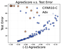
(b) AgreeScore.

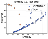
(c) Entropy.

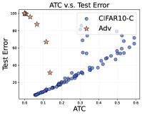
(d) ATC.

Figure 21: Evaluation of existing methods on predicting OOD error under adversarial attack. Blue circles are results evaluated on CIFAR10-C (each point corresponds to one corrupted test dataset), and orange stars are results evaluated on adversarial examples (each point corresponds to one perturbation radius $\varepsilon$).

Appendix F Proof of Proposition 4.4

Proof.

Recall that we decompose the empirical covariance of training and test set as

$${\boldsymbol{\Sigma}}=\frac{1}{n}{\boldsymbol{X}}^{\mathsf{T}}{\boldsymbol{X}}=\frac{1}{n}\sum_{i=1}^{n}\mu_{i}{\boldsymbol{u}}_{i}{\boldsymbol{u}}_{i}^{\mathsf{T}},$$

$$\widetilde{\boldsymbol{\Sigma}}=\frac{1}{m}\widetilde{\boldsymbol{X}}^{\mathsf{T}}\widetilde{\boldsymbol{X}}=\frac{1}{m}\sum_{j=1}^{m}\lambda_{j}{\boldsymbol{v}}_{j}{\boldsymbol{v}}_{j}^{\mathsf{T}}.$$

Then given $k$ from Assumption 4.3, we define the projection matrices

$${\boldsymbol{P}}_{0} =\sum_{i=1}^{k}{\boldsymbol{u}}_{i}{\boldsymbol{u}}_{i}^{\mathsf{T}}=\sum_{j=1}^{k}{\boldsymbol{v}}_{j}{\boldsymbol{v}}_{j}^{\mathsf{T}},$$

$${\boldsymbol{P}}_{\perp} ={\boldsymbol{P}}-{\boldsymbol{P}}_{0}=\sum_{i=k+1}^{n}{\boldsymbol{u}}_{i}{\boldsymbol{u}}_{i}^{\mathsf{T}},$$

$$\widetilde{\boldsymbol{P}}_{\perp} =\widetilde{\boldsymbol{P}}-\widetilde{\boldsymbol{P}}_{0}=\sum_{j=k+1}^{m}{\boldsymbol{v}}_{j}{\boldsymbol{v}}_{j}^{\mathsf{T}}.$$

The test loss can be written as

$$\textsf{TestLoss}=\frac{1}{m}\|\widetilde{\boldsymbol{X}}({\boldsymbol{I}}-{\boldsymbol{P}}){\boldsymbol{\theta}}_{\star}\|_{2}^{2}=\frac{1}{m}\|\widetilde{\boldsymbol{X}}\widetilde{\boldsymbol{P}}({\boldsymbol{I}}-{\boldsymbol{P}}){\boldsymbol{\theta}}_{\star}\|_{2}^{2}.$$

Under Assumption 4.3,

$$\widetilde{\boldsymbol{P}}({\boldsymbol{I}}-{\boldsymbol{P}})=({\boldsymbol{P}}_{0}+\widetilde{\boldsymbol{P}}_{\perp})({\boldsymbol{I}}-{\boldsymbol{P}}_{0}-{\boldsymbol{P}}_{\perp})=\widetilde{\boldsymbol{P}}_{\perp}.$$

This allows us to simply write the test loss as

$$\textsf{TestLoss}=\frac{1}{m}\|\widetilde{\boldsymbol{X}}\widetilde{\boldsymbol{P}}_{\perp}{\boldsymbol{\theta}}_{\star}\|_{2}^{2}=\frac{1}{m}\sum_{j=k+1}^{m}\lambda_{j}\langle{\boldsymbol{v}}_{j},{\boldsymbol{\theta}}_{\star}\rangle^{2}.$$

Since $\lambda_{j}$ is a the decreasing sequence of eigenvalues

$$\frac{\lambda_{m}}{m}\sum_{j=k+1}^{m}\langle{\boldsymbol{v}}_{j},{\boldsymbol{\theta}}_{\star}\rangle^{2}\leq\textsf{TestLoss}\leq\frac{\lambda_{k+1}}{m}\sum_{j=k+1}^{m}\langle{\boldsymbol{v}}_{j},{\boldsymbol{\theta}}_{\star}\rangle^{2}.$$

Note that with Assumption 4.2

$$\sum_{j=k+1}^{m}\langle{\boldsymbol{v}}_{j},{\boldsymbol{\theta}}_{\star}\rangle^{2}=\|\widetilde{\boldsymbol{P}}_{\perp}{\boldsymbol{\theta}}_{\star}\|_{2}^{2}=\|{\boldsymbol{P}}_{\perp}{\boldsymbol{\theta}}_{\star}\|_{2}^{2}=\|{\boldsymbol{P}}{\boldsymbol{\theta}}_{\star}\|_{2}^{2}-\|{\boldsymbol{P}}_{0}{\boldsymbol{\theta}}_{\star}\|_{2}^{2}=\|{\boldsymbol{P}}{\boldsymbol{\theta}}_{\star}\|_{2}^{2}-\|\widetilde{\boldsymbol{P}}{\boldsymbol{P}}{\boldsymbol{\theta}}_{\star}\|_{2}^{2}=\textsf{ProjNormLinear}^{2}.$$

This completes the proof of Proposition 4.4. ∎

References

- Allen-Zhu et al. (2019) Allen-Zhu, Z., Li, Y., and Liang, Y. Learning and generalization in overparameterized neural networks, going beyond two layers. In Proceedings of the 33rd International Conference on Neural Information Processing Systems, pp. 6158–6169, 2019.
- Balasubramanian et al. (2011) Balasubramanian, K., Donmez, P., and Lebanon, G. Unsupervised supervised learning ii: Margin-based classification without labels. In Proceedings of the Fourteenth International Conference on Artificial Intelligence and Statistics, pp. 137–145. JMLR Workshop and Conference Proceedings, 2011.
- Bartlett et al. (2020) Bartlett, P. L., Long, P. M., Lugosi, G., and Tsigler, A. Benign overfitting in linear regression. Proceedings of the National Academy of Sciences, 117(48):30063–30070, 2020.
- Ben-David et al. (2007) Ben-David, S., Blitzer, J., Crammer, K., Pereira, F., et al. Analysis of representations for domain adaptation. Advances in neural information processing systems, 19:137, 2007.
- Ben-David et al. (2010) Ben-David, S., Blitzer, J., Crammer, K., Kulesza, A., Pereira, F., and Vaughan, J. W. A theory of learning from different domains. Machine learning, 79(1):151–175, 2010.
- Bowman et al. (2015) Bowman, S. R., Angeli, G., Potts, C., and Manning, C. D. A large annotated corpus for learning natural language inference. arXiv preprint arXiv:1508.05326, 2015.
- Carlini & Wagner (2017) Carlini, N. and Wagner, D. Adversarial examples are not easily detected: Bypassing ten detection methods. In Proceedings of the 10th ACM workshop on artificial intelligence and security, pp. 3–14, 2017.
- Chen et al. (2021) Chen, M., Goel, K., Sohoni, N. S., Poms, F., Fatahalian, K., and Ré, C. Mandoline: Model evaluation under distribution shift. In International Conference on Machine Learning, pp. 1617–1629. PMLR, 2021.
- Chuang et al. (2020) Chuang, C.-Y., Torralba, A., and Jegelka, S. Estimating generalization under distribution shifts via domain-invariant representations. In International Conference on Machine Learning, pp. 1984–1994. PMLR, 2020.
- Deng et al. (2009) Deng, J., Dong, W., Socher, R., Li, L.-J., Li, K., and Fei-Fei, L. Imagenet: A large-scale hierarchical image database. In 2009 IEEE conference on computer vision and pattern recognition, pp. 248–255. Ieee, 2009.
- Deng & Zheng (2021) Deng, W. and Zheng, L. Are labels always necessary for classifier accuracy evaluation? In Proceedings of the IEEE/CVF Conference on Computer Vision and Pattern Recognition, pp. 15069–15078, 2021.
- Deng et al. (2021) Deng, W., Gould, S., and Zheng, L. What does rotation prediction tell us about classifier accuracy under varying testing environments? arXiv preprint arXiv:2106.05961, 2021.
- Devlin et al. (2018) Devlin, J., Chang, M.-W., Lee, K., and Toutanova, K. Bert: Pre-training of deep bidirectional transformers for language understanding. arXiv preprint arXiv:1810.04805, 2018.
- Donmez et al. (2010) Donmez, P., Lebanon, G., and Balasubramanian, K. Unsupervised supervised learning i: Estimating classification and regression errors without labels. Journal of Machine Learning Research, 11(4), 2010.
- Du et al. (2019) Du, S., Lee, J., Li, H., Wang, L., and Zhai, X. Gradient descent finds global minima of deep neural networks. In International Conference on Machine Learning, pp. 1675–1685. PMLR, 2019.
- Ganin et al. (2016) Ganin, Y., Ustinova, E., Ajakan, H., Germain, P., Larochelle, H., Laviolette, F., Marchand, M., and Lempitsky, V. Domain-adversarial training of neural networks. The journal of machine learning research, 17(1):2096–2030, 2016.
- Garg et al. (2022) Garg, S., Balakrishnan, S., Lipton, Z. C., Neyshabur, B., and Sedghi, H. Leveraging unlabeled data to predict out-of-distribution performance. arXiv preprint arXiv:2201.04234, 2022.
- Geifman & El-Yaniv (2017) Geifman, Y. and El-Yaniv, R. Selective classification for deep neural networks. Advances in Neural Information Processing Systems, 30:4878–4887, 2017.
- Geirhos et al. (2018) Geirhos, R., Rubisch, P., Michaelis, C., Bethge, M., Wichmann, F. A., and Brendel, W. Imagenet-trained cnns are biased towards texture; increasing shape bias improves accuracy and robustness. In International Conference on Learning Representations, 2018.
- Glockner et al. (2018) Glockner, M., Shwartz, V., and Goldberg, Y. Breaking nli systems with sentences that require simple lexical inferences. In Proceedings of the 56th Annual Meeting of the Association for Computational Linguistics (Volume 2: Short Papers), pp. 650–655, 2018.
- Goodfellow et al. (2014) Goodfellow, I. J., Shlens, J., and Szegedy, C. Explaining and harnessing adversarial examples. arXiv preprint arXiv:1412.6572, 2014.
- Guillory et al. (2021) Guillory, D., Shankar, V., Ebrahimi, S., Darrell, T., and Schmidt, L. Predicting with confidence on unseen distributions. In Proceedings of the IEEE/CVF International Conference on Computer Vision, pp. 1134–1144, 2021.
- Guo et al. (2017) Guo, C., Pleiss, G., Sun, Y., and Weinberger, K. Q. On calibration of modern neural networks. In International Conference on Machine Learning, pp. 1321–1330. PMLR, 2017.
- Hastie et al. (2001) Hastie, T., Tibshirani, R., and Friedman, J. The Elements of Statistical Learning. Springer Series in Statistics. Springer New York Inc., New York, NY, USA, 2001.
- Hastie et al. (2020) Hastie, T., Montanari, A., Rosset, S., and Tibshirani, R. J. Surprises in high-dimensional ridgeless least squares interpolation, 2020.
- He et al. (2016) He, K., Zhang, X., Ren, S., and Sun, J. Deep residual learning for image recognition. In Proceedings of the IEEE conference on computer vision and pattern recognition, pp. 770–778, 2016.
- Hendrycks & Dietterich (2019) Hendrycks, D. and Dietterich, T. Benchmarking neural network robustness to common corruptions and perturbations. arXiv preprint arXiv:1903.12261, 2019.
- Hendrycks & Gimpel (2016) Hendrycks, D. and Gimpel, K. A baseline for detecting misclassified and out-of-distribution examples in neural networks. arXiv preprint arXiv:1610.02136, 2016.
- Hendrycks et al. (2020) Hendrycks, D., Liu, X., Wallace, E., Dziedzic, A., Krishnan, R., and Song, D. Pretrained transformers improve out-of-distribution robustness. In Proceedings of the 58th Annual Meeting of the Association for Computational Linguistics, pp. 2744–2751, 2020.
- Hendrycks et al. (2021a) Hendrycks, D., Basart, S., Mu, N., Kadavath, S., Wang, F., Dorundo, E., Desai, R., Zhu, T., Parajuli, S., Guo, M., et al. The many faces of robustness: A critical analysis of out-of-distribution generalization. In Proceedings of the IEEE/CVF International Conference on Computer Vision, pp. 8340–8349, 2021a.
- Hendrycks et al. (2021b) Hendrycks, D., Zhao, K., Basart, S., Steinhardt, J., and Song, D. Natural adversarial examples. In Proceedings of the IEEE/CVF Conference on Computer Vision and Pattern Recognition, pp. 15262–15271, 2021b.
- Jacot et al. (2018) Jacot, A., Gabriel, F., and Hongler, C. Neural tangent kernel: Convergence and generalization in neural networks. In Bengio, S., Wallach, H., Larochelle, H., Grauman, K., Cesa-Bianchi, N., and Garnett, R. (eds.), Advances in Neural Information Processing Systems, volume 31. Curran Associates, Inc., 2018. URL https://proceedings.neurips.cc/paper/2018/file/5a4be1fa34e62bb8a6ec6b91d2462f5a-Paper.pdf.
- Jiang et al. (2021) Jiang, Y., Nagarajan, V., Baek, C., and Kolter, J. Z. Assessing generalization of sgd via disagreement. arXiv preprint arXiv:2106.13799, 2021.
- Koehler et al. (2021) Koehler, F., Zhou, L., Sutherland, D. J., and Srebro, N. Uniform convergence of interpolators: Gaussian width, norm bounds and benign overfitting. In Beygelzimer, A., Dauphin, Y., Liang, P., and Vaughan, J. W. (eds.), Advances in Neural Information Processing Systems, 2021. URL https://openreview.net/forum?id=FyOhThdDBM.
- Koh et al. (2021) Koh, P. W., Sagawa, S., Marklund, H., Xie, S. M., Zhang, M., Balsubramani, A., Hu, W., Yasunaga, M., Phillips, R. L., Gao, I., et al. Wilds: A benchmark of in-the-wild distribution shifts. In International Conference on Machine Learning, pp. 5637–5664. PMLR, 2021.
- Krizhevsky et al. (2009) Krizhevsky, A., Hinton, G., et al. Learning multiple layers of features from tiny images. 2009.
- Kurakin et al. (2017) Kurakin, A., Goodfellow, I. J., and Bengio, S. Adversarial machine learning at scale. In International Conference on Learning Representations, 2017.
- Lee et al. (2019) Lee, J., Xiao, L., Schoenholz, S., Bahri, Y., Novak, R., Sohl-Dickstein, J., and Pennington, J. Wide neural networks of any depth evolve as linear models under gradient descent. Advances in neural information processing systems, 32:8572–8583, 2019.
- Lee et al. (2018) Lee, K., Lee, K., Lee, H., and Shin, J. A simple unified framework for detecting out-of-distribution samples and adversarial attacks. Advances in neural information processing systems, 31, 2018.
- Liang et al. (2018) Liang, S., Li, Y., and Srikant, R. Enhancing the reliability of out-of-distribution image detection in neural networks. In International Conference on Learning Representations, 2018.
- Liu et al. (2019) Liu, Y., Ott, M., Goyal, N., Du, J., Joshi, M., Chen, D., Levy, O., Lewis, M., Zettlemoyer, L., and Stoyanov, V. Roberta: A robustly optimized bert pretraining approach. arXiv preprint arXiv:1907.11692, 2019.
- Long et al. (2015) Long, M., Cao, Y., Wang, J., and Jordan, M. Learning transferable features with deep adaptation networks. In International conference on machine learning, pp. 97–105. PMLR, 2015.
- Loshchilov & Hutter (2016) Loshchilov, I. and Hutter, F. Sgdr: Stochastic gradient descent with warm restarts. arXiv preprint arXiv:1608.03983, 2016.
- Loshchilov & Hutter (2017) Loshchilov, I. and Hutter, F. Decoupled weight decay regularization. arXiv preprint arXiv:1711.05101, 2017.
- Madani et al. (2004) Madani, O., Pennock, D., and Flake, G. Co-validation: Using model disagreement on unlabeled data to validate classification algorithms. Advances in neural information processing systems, 17:873–880, 2004.
- Marelli et al. (2014) Marelli, M., Menini, S., Baroni, M., Bentivogli, L., Bernardi, R., Zamparelli, R., et al. A sick cure for the evaluation of compositional distributional semantic models. In Lrec, pp. 216–223. Reykjavik, 2014.
- McCoy et al. (2019) McCoy, T., Pavlick, E., and Linzen, T. Right for the wrong reasons: Diagnosing syntactic heuristics in natural language inference. In Proceedings of the 57th Annual Meeting of the Association for Computational Linguistics, pp. 3428–3448, 2019.
- Miller et al. (2020) Miller, J., Krauth, K., Recht, B., and Schmidt, L. The effect of natural distribution shift on question answering models. In International Conference on Machine Learning, pp. 6905–6916. PMLR, 2020.
- Naik et al. (2018) Naik, A., Ravichander, A., Sadeh, N., Rose, C., and Neubig, G. Stress test evaluation for natural language inference. In Proceedings of the 27th International Conference on Computational Linguistics, pp. 2340–2353, 2018.
- Nakkiran & Bansal (2020) Nakkiran, P. and Bansal, Y. Distributional generalization: A new kind of generalization. arXiv preprint arXiv:2009.08092, 2020.
- Pan et al. (2010) Pan, S. J., Tsang, I. W., Kwok, J. T., and Yang, Q. Domain adaptation via transfer component analysis. IEEE transactions on neural networks, 22(2):199–210, 2010.
- Quiñonero-Candela et al. (2008) Quiñonero-Candela, J., Sugiyama, M., Schwaighofer, A., and Lawrence, N. D. Dataset shift in machine learning. Mit Press, 2008.
- Ravichander et al. (2019) Ravichander, A., Naik, A., Rose, C., and Hovy, E. Equate: A benchmark evaluation framework for quantitative reasoning in natural language inference. In Proceedings of the 23rd Conference on Computational Natural Language Learning (CoNLL), pp. 349–361, 2019.
- Recht et al. (2019) Recht, B., Roelofs, R., Schmidt, L., and Shankar, V. Do imagenet classifiers generalize to imagenet? In International Conference on Machine Learning, pp. 5389–5400. PMLR, 2019.
- Santurkar et al. (2021) Santurkar, S., Tsipras, D., and Madry, A. Breeds: Benchmarks for subpopulation shift. In International Conference on Learning Representations, 2021.
- Shankar et al. (2021) Shankar, V., Dave, A., Roelofs, R., Ramanan, D., Recht, B., and Schmidt, L. Do image classifiers generalize across time? In Proceedings of the IEEE/CVF International Conference on Computer Vision, pp. 9661–9669, 2021.
- Simonyan & Zisserman (2014) Simonyan, K. and Zisserman, A. Very deep convolutional networks for large-scale image recognition. arXiv preprint arXiv:1409.1556, 2014.
- Steinhardt & Liang (2016) Steinhardt, J. and Liang, P. S. Unsupervised risk estimation using only conditional independence structure. Advances in Neural Information Processing Systems, 29:3657–3665, 2016.
- Sun et al. (2020) Sun, Y., Wang, X., Liu, Z., Miller, J., Efros, A., and Hardt, M. Test-time training with self-supervision for generalization under distribution shifts. In International Conference on Machine Learning, pp. 9229–9248. PMLR, 2020.
- Taori et al. (2020) Taori, R., Dave, A., Shankar, V., Carlini, N., Recht, B., and Schmidt, L. Measuring robustness to natural distribution shifts in image classification. In Advances in Neural Information Processing Systems (NeurIPS), 2020. URL https://arxiv.org/abs/2007.00644.
- Tripuraneni et al. (2021) Tripuraneni, N., Adlam, B., and Pennington, J. Covariate shift in high-dimensional random feature regression. arXiv preprint arXiv:2111.08234, 2021.
- Tsigler & Bartlett (2020) Tsigler, A. and Bartlett, P. L. Benign overfitting in ridge regression. arXiv preprint arXiv:2009.14286, 2020.
- Tzeng et al. (2017) Tzeng, E., Hoffman, J., Saenko, K., and Darrell, T. Adversarial discriminative domain adaptation. In Proceedings of the IEEE conference on computer vision and pattern recognition, pp. 7167–7176, 2017.
- Williams et al. (2017) Williams, A., Nangia, N., and Bowman, S. R. A broad-coverage challenge corpus for sentence understanding through inference. arXiv preprint arXiv:1704.05426, 2017.
- Wilson et al. (2017) Wilson, A. C., Roelofs, R., Stern, M., Srebro, N., and Recht, B. The marginal value of adaptive gradient methods in machine learning. In Proceedings of the 31st International Conference on Neural Information Processing Systems, pp. 4151–4161, 2017.
- Xu et al. (2021) Xu, K., Ren, T., Zhang, S., Feng, Y., and Xiong, C. Unsupervised out-of-domain detection via pre-trained transformers. CoRR, abs/2106.00948, 2021. URL https://arxiv.org/abs/2106.00948.
- Zhao et al. (2019) Zhao, H., Des Combes, R. T., Zhang, K., and Gordon, G. On learning invariant representations for domain adaptation. In International Conference on Machine Learning, pp. 7523–7532. PMLR, 2019.
- Zhou et al. (2020) Zhou, X., Nie, Y., Tan, H., and Bansal, M. The curse of performance instability in analysis datasets: Consequences, source, and suggestions. In Proceedings of the 2020 Conference on Empirical Methods in Natural Language Processing (EMNLP), pp. 8215–8228, 2020.
- Zou et al. (2019) Zou, D., Cao, Y., Zhou, D., and Gu, Q. Gradient descent optimizes over-parameterized deep relu networks. Machine learning, 2019.