An a posteriori error estimator for the spectral fractional power of the Laplacian

Abstract
We develop a novel a posteriori error estimator for the $L^{2}$ error committed by the finite element discretization of the solution of the fractional Laplacian. Our a posteriori error estimator takes advantage of the semi–discretization scheme using rational approximations which allow to reformulate the fractional problem into a family of non–fractional parametric problems. The estimator involves applying the implicit Bank–Weiser error estimation strategy to each parametric non–fractional problem and reconstructing the fractional error through the same rational approximation used to compute the solution to the original fractional problem. In addition we propose an algorithm to adapt both the finite element mesh and the rational scheme in order to balance the discretization errors. We provide several numerical examples in both two and three-dimensions demonstrating the effectivity of our estimator for varying fractional powers and its ability to drive an adaptive mesh refinement strategy.

Keywords: Finite element methods, A posteriori error estimation, Fractional partial differential equations, Adaptive refinement methods, Bank–Weiser error estimator
2020 Mathematics Subject Classification: 65N15, 65N30
Published journal article: https://doi.org/10.1016/j.cma.2023.115943

1 Introduction

Fractional partial differential equations (FPDEs) have gained in popularity during the last two decades and are now applied in a wide range of fields [78] such as anomalous diffusion [24, 44, 54, 59, 81], electromagnetism and geophysical electromagnetism [32, 90], phase fluids [9, 11, 58], porous media [11, 43, 22, 36], quasi-geostrophic flows [29] and spatial statistics [23, 77].

The main interest in fractional models lies in their ability to reproduce non-local behavior with a relatively small number of parameters [16, 42]. While this non-locality can be interesting from a modeling perspective, it also constitutes an ongoing challenge for numerical methods since applying standard approaches naturally leads to large dense linear systems that are computationally intractable.

In the last decade various numerical methods have been derived in order to circumvent the main issues associated with the application of standard numerical methods to FPDEs. The two main ones being the non–locality leading to dense linear systems and, for some particular definitions of the fractional operator, the evaluation of singular integrals [6, 8].

We focus on discretization schemes based on finite element methods, other methods can be found e.g. in [1, 73, 84]. Among the methods addressing the above numerical issues, we can cite: methods to efficiently solve eigenvalue problems [44], multigrid methods for performing efficient dense matrix–vector products [6, 8], hybrid finite element–spectral schemes [7], Dirichlet-to-Neumann maps (such as the Caffarelli–Silvestre extension) [14, 40, 48, 62, 81, 87], semigroups methods [50, 51, 86], rational approximation methods [2, 72, 74], Dunford–Taylor integrals [23, 25, 26, 28, 30, 34, 65, 74] (which can be considered as particular examples of rational approximation methods) and reduced basis methods [52, 53, 56].

Although we focus exclusively on the spectral definition of the fractional Laplacian, there is no unique definition of the fractional power of the Laplacian operator. The three most frequently found definitions of the fractional Laplacian are: the integral fractional Laplacian, defined from the principal value of a singular integral over the whole space $\mathbb{R}^{d}$ [6, 8, 27, 40, 55], the regional fractional Laplacian, defined by the same singular integral but over a bounded domain only [47, 59, 61, 80] and the spectral fractional Laplacian, defined from the spectrum of the standard Laplacian over a bounded domain [7, 15, 19, 50, 72, 79]. The different definitions are equivalent in the entire space $\mathbb{R}^{d}$, but this is no longer the case on a bounded domain [24, 59, 76, 78]. These definitions lead to significantly different mathematical problems associated with infinitesimal generators of different stochastic processes [78, 59].

Efficient methods for solving fractional problems typically rely on a combination of different discretization methods. For example, [30, 71] which are also the foundation of this work, combine a rational sum representation of the spectral fractional Laplacian with a standard finite element method in space. Both the quadrature scheme and the finite element method induce discretization errors. In order to achieve a solution to a given accuracy while avoiding wasted computational time, these errors need to be balanced.

A priori error estimation has been tackled for some definitions of the fractional Laplacian, such as the integral Laplacian [5, 6, 7, 24, 30, 67] and the spectral fractional Laplacian [14, 15, 19, 30, 79, 81]. Unlike the standard Laplacian equation, solutions to the fractional Laplacian problems often exhibit strong boundary layers even for smooth data, particularly when the fractional power is low [68]. These singularities lead to computational difficulties and have to be taken into account using, for example a priori geometric mesh refinement towards the boundary of the domain [5, 20, 27, 34, 62], or partition of unity enrichment [33]. We emphasize that [30] contains already an a priori error analysis in the $L^{2}$ norm for a combined rational sum finite element method that we use in this work.

A posteriori error estimation has also been considered in the literature on fractional equations. A simple residual based estimator is proposed for the integral fractional Laplacian in [6]. A similar idea is used in the context of non-local variational inequalities in [67, 82]. Gradient-recovery based a posteriori error estimation has been developed in the context of fractional differential equations in [91]. In [24, 48] the authors present another estimator, based on the solution to local problems on cylindrical stars, for the integral fractional Laplacian discretized using the Caffarelli–Silvestre extension. A weighted residual estimator is derived in [63] in the same context.

2 Contribution

The main contribution of this work is the derivation of a novel a posteriori error estimator for the combined rational finite element approximation of the spectral fractional Laplacian. It is a natural a posteriori counterpart to the a priori results developed in [30]. To our knowledge, our work is the first to propose an a posteriori error estimator for the spectral fractional Laplacian discretized using rational approximation techniques (as opposed to the Caffarelli-Silvestre extension).

Our work starts with rational approximation–based discretization methods. We are particularly interested in two of these methods: a method based on the quadrature rule for the Dunford–Taylor integral proposed in the seminal work [30] —we will refer to this method as "the BP method" in the following— and a method based on Best Uniform Rational Approximations, —"the BURA method"— applied for the first time to fractional partial differential equations in [71]. These methods decompose the original fractional problem into a set of independent parametric non–fractional problems. From this point we develop an associated set of independent non–fractional a posteriori error estimation problems. We compute the Bank–Weiser hierarchical estimators [21] of the error between each non–fractional parametric problem solution and its finite element discretization, then the fractional problem discretization error is estimated by the sum of the parametric contributions via the rational approximation. In addition, we propose an algorithm to adaptively refine the rational scheme. When two discretization methods are combined (here a rational scheme and a finite element method), the respective discretization errors must be balanced in order to prevent computational resources waste. The algorithm we propose is based on a computable a priori estimator for the rational scheme error and rational schemes are chosen on–the–fly to balance the rational and finite element error estimators.

Our method leads to a fully local and parallelizable solution technique for the spectral fractional Laplacian with computable $L^{2}$ error. Our method is valid for any finite element degree (however, for the sake of brevity we do not show results with higher degree finite elements) and for one, two and three dimensional problems [39].

We implement our method in DOLFINx [69], the new problem solving environment of the FEniCS Project [13]. A simple demonstration implementation is included in the supplementary material. We show numerical results demonstrating that the estimator can correctly reproduce the a priori convergence rates derived in [30]. Our newly developed error estimator is then used to steer an adaptive mesh refinement algorithm, resulting in improved convergence rates for small fractional powers and strong boundary layers.

3 Motivation

Given a fractional power $s$ in $(0,1)$ and a rational approximation $\mathcal{Q}_{s}(\lambda)$ of the function $\lambda^{-s}$, it is possible to construct a semi-discrete approximation $u_{\mathcal{Q}_{s}}$ of the solution $u$ to a fractional Laplace equation as a weighted sum of solutions $(u_{l})_{l}$ to non–fractional parametric problems. Then, a fully discrete approximation of $u$ is obtained by discretizing the parametric solutions $(u_{l})_{l}$ using a finite element method.

An a posteriori error estimator is then computed as the weighted sum of the Bank–Weiser estimators of the error between each $u_{l}$ and its finite element discretization. As we will see in the following, the resulting numerical scheme is simple and its implementation in code is straightforward. Furthermore it maintains the appealing parallel nature of rational approximation schemes [30, 65, 72].

We remark on why we have chosen to use the Bank–Weiser type error estimator, as opposed to one of the many other error estimation strategies, e.g. explicit residual, equilibrated fluxes, or recovery-type estimators (see [10, 46] and references therein). In the case of fractional powers of the Laplacian operator, the resulting set of parametric problems consists of singularly–perturbed reaction–diffusion equations. It has been proven in [89] that the Bank–Weiser estimator is robust with respect to the coefficients appearing in these parametric problems when the error is measured in the natural norm. To our knowledge, no such robustness, which our numerical experiments do indicate, has been established for the $L^{2}$-norm for the Bank–Weiser estimator. Nevertheless, our numerical experiments indicate that this does appear to be the case. Moreover, the Bank–Weiser estimator can be straightforwardly applied to higher-order finite element methods and higher-dimension problems. In addition, its computational stencil is highly local which is particularly appealing for three-dimensional problems see e.g. [39]. Finally, our choice of the Bank–Weiser estimator is also justified in section 6.2.1.

In this work we focus on error estimation in the $L^{2}$ norm, the estimation of the error in the ‘natural’ fractional norm is the topic of ongoing work. For simplicity, we only consider fractional powers of the Laplacian with homogeneous Dirichlet boundary conditions.

4 Problem statement

For any subset $\omega$ of $\overline{\Omega}$ we denote $L^{2}(\omega)$ the space of square integrable functions on $\omega$ and $\left(\cdot,\cdot\right)_{\omega}$ its usual inner product. Let $H^{1}(\omega)$ be the Sobolev space of functions with first order weak derivatives in $L^{2}(\omega)$. The space $H^{1}(\omega)$ is endowed with the usual inner product $\left(\nabla\cdot,\nabla\cdot\right)_{L^{2}(\omega)}+\left(\cdot,\cdot\right)_{L^{2}(\omega)}$. We will omit the dependence in $\omega$ in the subscripts when $\omega=\Omega$. We will make use of the notation $\partial v/\partial n:=\nabla v\cdot n$ for the normal derivative of a smooth enough function $v$. We denote $H^{1}_{0}(\Omega)$ the subspace of functions in $H^{1}(\Omega)$ with a zero trace on $\Gamma$.

We consider the family of eigenfunctions $\{\psi_{i}\}_{i=1}^{\infty}\subset H^{1}_{0}(\Omega)$ of the standard Laplacian operator with uniform zero Dirichlet boundary condition on $\Omega$ as well as the corresponding family of eigenvalues $\{\lambda_{i}\}_{i=1}^{\infty}$ such that

$$\left(\nabla\psi_{i},\nabla v\right)=\lambda_{i}\left(\psi_{i},v\right),\quad\forall v\in H^{1}_{0}(\Omega),\ \forall i\in[\![1,+\infty[\![.$$ (1)

We assume the Laplacian eigenvalues are sorted in increasing order and we assume $\lambda_{0}\in\mathbb{R}$ is a lower bound of the spectrum

$$\lambda_{0}\leqslant\lambda_{1}\leqslant\cdots\leqslant\lambda_{i}\leqslant\lambda_{i+1}\leqslant\cdots$$ (2)

The family $\{\psi_{i}\}_{i=1}^{\infty}$ is an orthonormal basis of $L^{2}(\Omega)$ [12]. For $s$ in $(0,1)$ we introduce the spectral fractional Sobolev space $\mathbb{H}^{s}$ and its natural norm

$$\mathbb{H}^{s}:=\left\{v\in L^{2}(\Omega),\ \sum_{i=1}^{\infty}\lambda_{i}^{s}\left(v,\psi_{i}\right)^{2}<\infty\right\},\qquad\lVert v\rVert_{\mathbb{H}^{s}}^{2}:=\sum_{i=1}^{\infty}\lambda_{i}^{s}\left(v,\psi_{i}\right)^{2}.$$ (3)

Especially, for $0\leqslant s\leqslant 1$ we have $H^{1}_{0}(\Omega)=\mathbb{H}^{1}(\Omega)\subseteq\mathbb{H}^{s}(\Omega)\subseteq L^{2}(\Omega)=:\mathbb{H}^{0}(\Omega)$ and the norm $\lVert\cdot\rVert_{\mathbb{H}^{s}}$ coincide with $\lVert\cdot\rVert_{L^{2}}$ when $s=0$ and with $\lvert\cdot\rvert_{H^{1}}$ when $s=1$. In the following, for a function $v\in L^{2}(\Omega)$ we will denote $v_{i}:=\left(v,\psi_{i}\right)$ for all $i\geqslant 1$.

4.1 The spectral fractional Laplacian

Let $s$ be a real number in $(0,1)$ and $f$ be a given function in $L^{2}(\Omega)$. We consider the following fractional Laplacian problem: we look for a function $u$ such that

$$\mathcal{L}^{s}u=f,$$ (4)

where $\mathcal{L}$ stands for the Laplacian operator in $\Omega$, with homogeneous Dirichlet boundary conditions on $\Gamma$. Let us consider $\{\lambda_{i},\psi_{i}\}_{i=1}^{+\infty}\subset\mathbb{R}^{+*}\times L^{2}(\Omega)$, the spectrum of $\mathcal{L}$, defined by the following generalized eigenvalue problem

$$\left(\nabla\psi_{i},\nabla v\right)=\lambda_{i}\left(\psi_{i},v\right),\quad\forall v\in H^{1}_{0}(\Omega),\ \forall i\in\llbracket 1,+\infty\llbracket.$$ (5)

The solution $u$ of eq. 4 is defined using the spectrum of the standard Laplacian [15]

$$\left(u,v\right):=\left(\mathcal{L}^{-s}f,v\right)=\sum_{i=1}^{\infty}\lambda_{i}^{-s}f_{i}\left(\psi_{i},v\right),\quad\forall v\in H^{1}_{0}(\Omega).$$ (6)

If we notice that

$$u_{i}=\lambda_{i}^{-s}f_{i},\qquad\forall i\geqslant 1,$$ (7)

then, for $f$ in $L^{2}(\Omega)$ we can show that

$$\lVert u\rVert_{\mathbb{H}^{2s}}=\lVert f\rVert_{L^{2}}.$$ (8)

4.2 Rational approximation

Our method relies on rational approximations of the real function $\lambda\mapsto\lambda^{-s}$ for $\lambda\geqslant\lambda_{0}$ where $\lambda_{0}>0$ is a fixed lower bound and for $s$ in $(0,1)$. We present here the two examples we are interested in: the BP method introduced in [30] and the BURA method presented in [71].

Both these methods are rational approximation methods; they aim at approximating the function $\lambda\mapsto\lambda^{-s}$ by a rational function of the form

$$\mathcal{Q}_{s}(\lambda):=C_{1}(s,N)+C_{2}(s,N)\sum_{l=-M}^{N}\frac{a_{l}(s,N)}{c_{l}(s,N)+b_{l}(s,N)\lambda},$$ (9)

where $M,N,C_{1},C_{2},(a_{l})_{l=1}^{N},(b_{l})_{l=1}^{N}$ and $(c_{l})_{l=1}^{N}$ are properly chosen parameters. Many rational approximation schemes have been proposed in the literature, see e.g. [2, 3, 64, 72, 88].

Before we present the two particular schemes we used in our numerical experiments, we want to highlight again that the error estimation scheme developed later can be derived in the same manner regardless of the choice of the rational approximation, as long as it leads to a set of well–posed non–fractional parametric problems.

4.2.1 The BP method

The BP method is based on the following expression derived from the Balakrishnan’s formula [17]

$$\lambda^{-s}=\frac{2\sin(\pi s)}{\pi}\int_{-\infty}^{+\infty}\operatorname{e}^{2sy}\left(1+\operatorname{e}^{2y}\lambda\right)^{-1}\ \,\mathrm{d}y.$$ (10)

Then, the rational approximation is obtained from eq. 10 by discretizing the integral on the right-hand side with a trapezoidal quadrature rule,

$$\mathcal{Q}_{s}(\lambda):=\frac{2\kappa\sin(\pi s)}{\pi}\sum_{l=-M(\kappa)}^{N(\kappa)}\operatorname{e}^{2sl\kappa}\left(1+\operatorname{e}^{2l\kappa}\lambda\right)^{-1},$$ (11)

where $\kappa>0$ is the fineness parameter and

$$M(\kappa):=\left\lceil\frac{\pi^{2}}{4s\kappa^{2}}\right\rceil,\quad\text{and}\quad N(\kappa):=\left\lceil\frac{\pi^{2}}{4(1-s)\kappa^{2}}\right\rceil,$$ (12)

where $\lceil\cdot\rceil$ is the ceiling function. Thus,

$$\lim_{\kappa\to 0}\mathcal{Q}_{s}(\lambda)=\lambda^{-s},\quad\forall(\lambda,s)\in[\lambda_{0},+\infty)\times(0,1).$$ (13)

The convergence of the BP method has been studied in [30, 28]. Especially, it has been proved that $\mathcal{Q}_{s}$ converges uniformly to $\lambda\mapsto\lambda^{-s}$ at an exponential rate as $\kappa$ tends to zero. The method has been applied to the discretization of various types of PDEs in e.g. [30, 31, 26, 25].

4.2.2 The BURA method

The starting point of the BURA method is the approximation of the function $g(\lambda)=\lambda^{s}$ for $\lambda\in[0,\lambda_{0}^{-1}]$. In this study we used the novel algorithm from [75] to compute the residuals and poles of the BURA of $g(\lambda)$. From this algorithm we obtain the following rational approximation

$$\mathcal{R}_{s}(\lambda):=\mathcal{R}_{s}(0)+\sum_{l=1}^{N}\frac{r_{l}}{p_{l}}+\sum_{l=1}^{N}\frac{r_{l}}{\lambda-p_{l}},$$ (14)

where $N$ is the degree of the rational function, $(r_{l})_{l=1}^{N}\subset\mathbb{R}^{+*}$ are its residuals and $(p_{l})_{l=1}^{N}\subset\mathbb{R}^{-*}$ its poles. Especially, if $\mathbb{P}_{N}$ is the space of polynomial functions of degree $N$ on $(0,\lambda_{0}^{-1}]$ and

$$\mathbb{Q}_{N}=\left\{\frac{p}{q},\ p,q\in\mathbb{P}_{N},q\neq 0\right\},$$ (15)

is the space of rational functions of degree $N$ over $(0,\lambda_{0}^{-1}]$, then

$$\mathcal{R}_{s}\simeq\operatorname*{arg\,min}_{\widetilde{r}\in\mathbb{Q}_{N}}\lVert g-\widetilde{r}\rVert_{L^{\infty}(0,\lambda_{0}^{-1}]}.$$ (16)

See [75] for a detailed discussion.

Then, an approximation of $\lambda\mapsto\lambda^{-s}$ can be obtained using partial fraction decomposition

$$\mathcal{Q}_{s}(\lambda):=\mathcal{R}_{s}(\lambda^{-1}) =\mathcal{R}_{s}(0)+\sum_{l=1}^{N}\frac{r_{l}}{p_{l}}+\sum_{l=1}^{N}\frac{r_{l}}{\lambda^{-1}-p_{l}}$$

$$=\mathcal{R}_{s}(0)+\sum_{l=1}^{N}\frac{r_{l}p_{l}+r_{l}(\lambda^{-1}-p_{l})}{p_{l}(\lambda^{-1}-p_{l})}$$

$$=\mathcal{R}_{s}(0)+\sum_{l=1}^{N}\frac{r_{l}}{p_{l}(1-p_{l}\lambda)}.$$ (17)

Like for the BP method, the convergence of the BURA method is of exponential rate, as proved in [85]. However, numerical evidence in the literature show that the BURA method is more efficient than the BP method (see e.g. [74]). In particular, it leads to a lowest number of parametric solves for a given accuracy. For more detailed discussions on BURA methods, see e.g. [2, 72, 74, 75].

5 Discretization

We combine the rational approximation eq. 9 with a finite element method to derive a fully discrete approximation of the solution $u$ to eq. 4.

5.1 Rational semi-discrete approximation

The general scheme used for the semi–discrete approximation will be replaced by the BP method eq. 11 and the BURA method eq. 17 in the numerical experiments of section 9.

We define a semi–discrete approximation of the solution $u$, defined in eq. 6 by replacing $\lambda_{i}^{-s}$ by $\mathcal{Q}_{s}(\lambda_{i})$ in eq. 6. Thus,

$$\left(u_{\mathcal{Q}_{s}},v\right):=\sum_{i=1}^{+\infty}\left(C_{1}+C_{2}\sum_{l=-M}^{N}\frac{a_{l}}{c_{l}+b_{l}\lambda_{i}}\right)f_{i}\left(\psi_{i},v\right),\quad\forall v\in H^{1}_{0}(\Omega).$$ (18)

If we interchange the two sums in eq. 18, we obtain

$$\left(u_{\mathcal{Q}_{s}},v\right)=C_{1}\left(f,v\right)+C_{2}\sum_{l=-M}^{N}a_{l}\left(u_{l},v\right),\quad\forall v\in H^{1}_{0}(\Omega),$$ (19)

where the functions $\{u_{l}\}_{l=-M}^{N}$ are solutions to the parametric problems: for each $l$ in $\llbracket-M,N\rrbracket$, find $u_{l}$ in $H^{1}_{0}$ such that

$$c_{l}\left(u_{l},v\right)+b_{l}\left(\nabla u_{l},\nabla v\right)=\left(f,v\right),\quad\forall v\in H^{1}_{0}(\Omega).$$ (20)

Note, eq. 19 can be written as

$$u_{\mathcal{Q}_{s}}=C_{1}f+C_{2}\sum_{l=-M}^{N}a_{l}u_{l}.$$ (21)

Since the family of eigenfunctions of the Laplacian $\{\psi_{i}\}_{i=1}^{+\infty}\subset H^{1}_{0}(\Omega)$ is a Hilbert basis of $L^{2}(\Omega)$, the space $H^{1}_{0}(\Omega)$ is dense in $L^{2}(\Omega)$ and the orthogonal projection of $f$ onto $H^{1}_{0}(\Omega)$ in eq. 19 is $f$ itself.

Using eq. 19, we reduce the problem eq. 4 to a series of parametric non–fractional problems eq. 20 to solve. As we will see in section 9, the number of parametric problems to solve can be relatively small, especially when the BURA method is used in the semi–discrete approximation. Moreover, these non–fractional problems are fully independent from each other so their solve can be performed in parallel.

5.2 Finite element discretization

In order to get a fully discrete approximation of $u$, we use a finite element method to discretize the parametric problems eq. 20. Although it is not mandatory, we use the same mesh and same finite element space for all the parametric problems. We discuss this choice, and possible alternative strategies, in section 7.1.

Let $\mathcal{T}$ be a mesh on the domain $\Omega$, composed of cells $\mathcal{T}=\left\{T\right\}$, facets $\mathcal{E}=\left\{E\right\}$ (we call facets the edges in dimension two and the faces in dimension three), and vertices. The mesh $\mathcal{T}$ is supposed to be regular, in Ciarlet’s sense: $h_{T}/\rho_{T}\leqslant\gamma,\ \forall T\in\mathcal{T}$, where $h_{T}$ is the diameter of a cell $T$, $\rho_{T}$ the diameter of its inscribed ball, and $\gamma$ is a positive constant fixed once and for all. The subset of facets that are not coincident with the boundary $\Gamma$ (called interior facets) is denoted $\mathcal{E}_{I}$. Let $n^{+}$ and $n^{-}$ in $\mathbb{R}^{d}$ be the outward unit normals to a given edge as seen by two cells $T^{+}$ and $T^{-}$ incident to a common edge $E$. The space of polynomials of order $p$ on a cell $T$ is denoted $\mathcal{P}_{p}(T)$ and the continuous Lagrange finite element space of order $p$ on the mesh $\mathcal{T}$ is defined by

$$V^{p}:=\left\{v_{p}\in H^{1}(\Omega),v_{p|T}\in\mathcal{P}_{p}(T)\;\forall T\in\mathcal{T}\right\}.$$ (22)

We denote $V^{p}_{0}$ the finite element space composed by functions of $V^{p}$ vanishing on the boundary $\Gamma$. For a given index $l$, the finite element discretization of eq. 20 reads: for each $l$ in $\llbracket-M,N\rrbracket$, find $u_{l,p}$ in $V^{p}_{0}$ such that

$$c_{l}\left(u_{l,p},v_{p}\right)+b_{l}\left(\nabla u_{l,p},\nabla v_{p}\right)=\left(f,v_{p}\right),\quad\forall v_{p}\in V^{p}_{0}.$$ (23)

Then, combining the solutions to eq. 23 as in eq. 18 we can give a fully discrete approximation of the solution to eq. 4 $u_{\mathcal{Q}_{s},p}\in V^{p}_{0}$, such that

$$\left(u_{\mathcal{Q}_{s},p},v_{p}\right)=C_{1}\left(f,v_{p}\right)+C_{2}\sum_{l=-M}^{N}a_{l}\left(u_{l,p},v_{p}\right),\quad\forall v_{p}\in V^{p}_{0}.$$ (24)

Note, eq. 24 can be rewritten as

$$u_{\mathcal{Q}_{s},p}=C_{1}f_{V^{p}_{0}}+C_{2}\sum_{l=-M}^{N}a_{l}u_{l,p},$$ (25)

where $f_{V^{p}_{0}}$ is the $L^{2}$ projection of $f$ onto the finite element space $V^{p}_{0}$. The computation of $u_{\mathcal{Q}_{s},p}$ is summarized in the top part of fig. 1. For a detailed discussion on the derivation of $u_{\mathcal{Q}_{s},p}$ in terms of matrices, see [74].

6 Error analysis

This section aims at studying the total discretization error defined by

$$e:=\lVert u-u_{\mathcal{Q}_{s},p}\rVert_{L^{2}}.$$ (26)

Since for any $s\in(0,1)$, the discrepancy $u-u_{\mathcal{Q}_{s},p}$ belongs to $\mathbb{H}^{2s}(\Omega)\subset L^{2}(\Omega)$, the error can be measured in the $L^{2}$ norm for any value of the fractional power $s$.

Using the triangle inequality, $e$ is controlled from above by the sum of the rational discretization error $\lVert u-u_{\mathcal{Q}_{s}}\rVert_{L^{2}}$ and the finite element discretization error $\lVert u_{\mathcal{Q}_{s}}-u_{\mathcal{Q}_{s},p}\rVert_{L^{2}}$ as follow

$$e=\lVert u-u_{\mathcal{Q}_{s},p}\rVert_{L^{2}}=\lVert u-u_{\mathcal{Q}_{s}}+u_{\mathcal{Q}_{s}}-u_{\mathcal{Q}_{s},p}\rVert_{L^{2}}\leqslant\lVert u-u_{\mathcal{Q}_{s}}\rVert_{L^{2}}+\lVert u_{\mathcal{Q}_{s}}-u_{\mathcal{Q}_{s},p}\rVert_{L^{2}}$$ (27)

In the following we describe estimators for each contribution however the main novelty of this study comes from the finite element discretization error estimation.

6.1 Rational approximation error analysis

The estimation of the error induced by the approximation of $u$ by $u_{\mathcal{Q}_{s}}$ reduces to the estimation of the scalar rational approximation error. First, we notice that, if we take $v=\psi_{i}$ in eq. 18, the coefficients $u_{\mathcal{Q}_{s},i}$ of $u_{\mathcal{Q}_{s}}$ in the basis $\{\psi_{i}\}_{i=1}^{+\infty}$ are given by

$$u_{\mathcal{Q}_{s},i}=\mathcal{Q}_{s}(\lambda_{i})f_{i},\qquad\forall i\geqslant 1.$$ (28)

Then, using the expansion in the basis $\{\psi_{i}\}_{i=1}^{+\infty}$, eq. 6 and eq. 28 we have

$$\lVert u-u_{\mathcal{Q}_{s}}\rVert_{L^{2}}^{2} =\sum_{i=1}^{+\infty}(u_{i}-u_{\mathcal{Q}_{s},i})^{2}$$

$$=\sum_{i=1}^{+\infty}\left(\lambda_{i}^{-s}-\mathcal{Q}_{s}(\lambda_{i})\right)^{2}f_{i}^{2}$$

$$\leqslant\max_{\lambda\geqslant\lambda_{0}}(\lambda^{-s}-\mathcal{Q}_{s}(\lambda))^{2}\lVert f\rVert_{L^{2}}^{2}.$$

So,

$$\lVert u-u_{\mathcal{Q}_{s}}\rVert_{L^{2}}\leqslant\max_{\lambda\geqslant\lambda_{0}}(|\lambda^{-s}-\mathcal{Q}_{s}(\lambda)|)\lVert f\rVert_{L^{2}}.$$ (29)

Thus, the following rational approximation error estimator

$$\eta_{\mathcal{Q}_{s}}=\max_{\lambda_{0}\leqslant\lambda\leqslant\lambda^{+}}(|\lambda^{-s}-\mathcal{Q}_{s}(\lambda)|)\lVert f\rVert_{L^{2}},$$ (30)

for a large value of $\lambda^{+}$, is cheap to compute since it consists in the approximation of the maximum of a scalar function and the approximation of the $L^{2}$ norm of the data $f$. In addition, we emphasize that this estimator does not require the discrete solution $u_{\mathcal{Q}_{s},p}$ unlike the finite element error estimator we describe in the next section. However, $\eta_{\mathcal{Q}_{s}}$ depends on the lower bound of the Laplacian spectrum $\lambda_{0}$ and thus can be optimized by taking $\lambda_{0}=\lambda_{1}$ when $\lambda_{1}$ is known. When it is not the case, precise guaranteed lower bounds for $\lambda_{1}$ could be obtained following e.g. [41, 45].

6.2 Finite element discretization error analysis

Our goal is to derive a quantity $\eta$, depending on $f$ and the finite element approximations $(u_{l,p})_{l=-M}^{N}$ such that

$$\eta\simeq\lVert u_{\mathcal{Q}_{s}}-u_{\mathcal{Q}_{s},p}\rVert_{L^{2}}.$$ (31)

Our method is based on the Bank–Weiser finite element error estimator introduced in [21] and its implementation in the FEniCSx software described in [39].

6.2.1 Heuristics

Let us start with some heuristics motivating the derivation of our a posteriori error estimator. The main idea is to derive a function $e^{\mathrm{bw}}_{\mathcal{Q}_{s},T}$ that locally represents the discretization error in the solution to the fractional problem $(u_{\mathcal{Q}_{s}}-u_{\mathcal{Q}_{s},p})_{|T}$ on a cell $T$ of the mesh. Combining eq. 19 and eq. 25, on a cell $T$ of the mesh we have

$$(u_{\mathcal{Q}_{s}}-u_{\mathcal{Q}_{s},p})_{|T}=C_{1}(f-f_{V^{p}_{0}})_{|T}+C_{2}\sum_{l=-M}^{N}a_{l}(u_{l}-u_{l,p})_{|T}.$$ (32)

We approximate the difference $f-f_{V^{p}_{0}}$ by $f_{\overline{V}}-f_{V^{p}_{0}}$ where $f_{\overline{V}}$ is the $L^{2}$ projection of $f$ onto a finer finite element space $\overline{V}$ (e.g. we can choose $\overline{V}:=V^{p+1}$). Note that this step is not necessary in the BP method since the projection of $f$ onto $V^{p}_{0}$ is not involved in the rational sum.

To approximate the differences $(u_{l}-u_{l,p})_{l=-M}^{N}$ we can use the framework proposed by Bank and Weiser in [21] to derive solutions $e^{\mathrm{bw}}_{l,T}$ such that

$$e^{\mathrm{bw}}_{l,T}\simeq(u_{l}-u_{l,p})_{|T},\quad\forall l\in\llbracket-M,N\rrbracket,\ \forall T\in\mathcal{T}.$$ (33)

We obtain $e^{\mathrm{bw}}_{\mathcal{Q}_{s},T}$ using the rational approximation sum

$$e^{\mathrm{bw}}_{\mathcal{Q}_{s},T}:=C_{1}(f_{\overline{V}}-f_{V^{p}_{0}})_{|T}+C_{2}\sum_{l=-M}^{N}a_{l}e^{\mathrm{bw}}_{l,T}\simeq(u_{\mathcal{Q}_{s}}-u_{\mathcal{Q}_{s},p})_{|T},\quad\forall T\in\mathcal{T}.$$ (34)

Finally, we can estimate the $L^{2}$ error on the cell $T$ by taking the norm of the function $e^{\mathrm{bw}}_{\mathcal{Q}_{s},T}$

$$\lVert e^{\mathrm{bw}}_{\mathcal{Q}_{s},T}\rVert_{L^{2}}\simeq\lVert(u_{\mathcal{Q}_{s}}-u_{\mathcal{Q}_{s},p})_{|T}\rVert_{L^{2}}.$$ (35)

The heuristic of the approximation of the parametric errors $(u_{l}-u_{l,p})_{l=-M}^{N}$ is summarized in fig. 1.

We would like to emphasize that the Bank–Weiser estimator is not the only possible choice. In fact, the Bank–Weiser estimator could be replaced with another estimator based on the solves of local problems, such as e.g. the one used in [81].

6.2.2 A posteriori error estimation

Let us now derive our a posteriori error estimation method more precisely. As mentioned in the last subsection, this estimator is based on a hierarchical estimator computed from the solves of local Neumann problems on the cells and introduced for the first time by Bank and Weiser in [21].

Let $T$ be a cell of the mesh. We make use of the following local finite element spaces

$$V^{p}_{T}:=\left\{v_{p,T}\in\mathcal{P}_{p}(T),\ v_{p,T}=0\ \text{in}\ (\Omega\setminus\overline{T})\cup(\overline{T}\cap\partial\Omega)\right\}.$$ (36)

Let us now consider two non-negative integers $p_{+}$ and $p_{-}$ such that $p_{+}>p_{-}\geqslant 0$ and $\mathcal{L}_{T}:V^{p_{+}}_{T}\longrightarrow V^{p_{-}}_{T}$ the local Lagrange interpolation operator. We introduce the local Bank–Weiser space, defined by

$$V^{\mathrm{bw}}_{T}:=\ker(\mathcal{L}_{T})=\left\{v_{p_{+},T}\in V^{p_{+}}_{T},\ \mathcal{L}_{T}(v_{p_{+},T})=0\right\}.$$ (37)

The local parametric Bank–Weiser problem associated to the parametric problems eq. 20 and eq. 23 reads

$$\int_{T}e^{\mathrm{bw}}_{l,T}v^{\mathrm{bw}}_{T}+\operatorname{e}^{2l\kappa}\int_{T}\nabla e^{\mathrm{bw}}_{l,T}\cdot\nabla v^{\mathrm{bw}}_{T}=\int_{T}r_{l,T}v^{\mathrm{bw}}_{T}-\frac{1}{2}\sum_{E\in\partial T}\int_{E}J_{l,E}v^{\mathrm{bw}}_{T},\ \forall v^{\mathrm{bw}}_{T}\in V^{\mathrm{bw}}_{T}$$ (38)

where $r_{l,T}$ and $J_{l,T}$ are defined as follow:

$$r_{l,T}:=f_{|T}-{u_{l,p}}_{|T}+\operatorname{e}^{2l\kappa}\Delta{u_{l,p}}_{|T},\quad\text{and}\quad J_{l,T}:=\operatorname{e}^{2l\kappa}\left(\frac{\partial u_{l,p|T_{+}}}{\partial n}-\frac{\partial u_{l,p|T_{-}}}{\partial n}\right),$$ (39)

where $T_{+}$ and $T_{-}$ are the cells sharing the edge $E$ such that the normal $n$ is outward $T_{+}$. The solution $e^{\mathrm{bw}}_{l,T}$ in $V^{\mathrm{bw}}_{T}$ is the local parametric Bank–Weiser solution. More details about the computation and implementation of the Bank–Weiser solutions can be found in [21, 39].

Then, we derive the local fractional Bank–Weiser solution by summing the local parametric Bank–Weiser solutions into the rational approximation sum

$$e_{\mathcal{Q}_{s},T}^{\mathrm{bw}}:=C_{1}(f_{\overline{V}}-f_{V^{p}_{0}})_{|T}+C_{2}\sum_{l=-M}^{N}a_{l}e_{l,T}^{\mathrm{bw}}.$$ (40)

The local fractional Bank–Weiser estimator is then defined as the $L^{2}$ norm of this local solution

$$\eta^{\mathrm{bw}}_{\mathcal{Q}_{s},T}:=\lVert e_{\mathcal{Q}_{s},T}^{\mathrm{bw}}\rVert_{L^{2}(T)}.$$ (41)

The global fractional Bank–Weiser estimator is then defined by

$${\eta^{\mathrm{bw}}_{\mathcal{Q}_{s}}}^{2}:=\sum_{T\in\mathcal{T}}{\eta^{\mathrm{bw}}_{\mathcal{Q}_{s},T}}^{2}.$$ (42)

Figure 1: Summary of the computation of the fractional solution approximation and of the fractional Bank–Weiser solution.

7 Adaptive refinement

One of the main applications of a posteriori error estimation is to drive adaptive mesh refinement algorithms. When the error is unevenly spread across the mesh, refining uniformly is a waste of computational resources leading to suboptimal convergence rates in the number of degrees of freedom. This problem is compounded for computationally expensive problems like fractional problems. Moreover, it is known that fractional problems often show a boundary layer behavior, the discretization error is consequently large in a localized region near the boundary [4, 35, 88]. This problem has been tackled using graded meshes that are refined near the boundary based on a priori or a posteriori considerations [24, 48, 67, 79]. As expected, the use of graded meshes improves the convergence of the methods.

Adaptive refinement algorithms are based on the loop

$$\cdots\longrightarrow\mathrm{Solve}\longrightarrow\mathrm{Estimate}\longrightarrow\mathrm{Mark}\longrightarrow\mathrm{Refine}\longrightarrow\cdots$$

In this work we are concerned with developments in the modules solve, estimate and, when an adaptive rational scheme is used, the module refine.

In section 7.1, we focus on the finite element mesh adaptive refinement, choosing a fixed rational scheme fine enough for the rational approximation error to be negligible. We are using the Dörfler algorithm [57] for the mark module and the Plaza–Carey algorithm [83] for the refine module.

In section 7.2, we allow the rational scheme to vary from one refinement step to another, in order to balance the discretization errors. Thus, the refine module is composed of the Plaza–Carey algorithm for the finite element mesh and an algorithm in charge of picking the right rational scheme in order for the rational and finite element approximation errors to be balanced at each refinement step.

Rational approximation methods have the advantage of being fully parallelizable due to the independence of the parametric problems from each other. Similarly, the local a posteriori error estimation method we have presented earlier is also parallelizable since the computation of the local Bank–Weiser solutions on the cells are independent from each other. Our error estimation strategy combines these advantages and is fully parallelizable both with respect to the parametric problems and local estimators computation.

7.1 Finite element mesh adaptive refinement

An example of error estimation and mesh adaptive refinement algorithm based on our method is shown in fig. 2. In this algorithm, we focus on the finite element error approximation. Thus, the rational scheme is fixed and chosen so that the rational approximation error is negligible. In this context, we assume that the total discretization error satisfies

$$\lVert u-u_{\mathcal{Q}_{s},p}\rVert_{L^{2}}\simeq\lVert u_{\mathcal{Q}_{s}}-u_{\mathcal{Q}_{s},p}\rVert_{L^{2}}.$$ (43)

Choose a tolerance $\varepsilon>0$, an initial mesh $\mathcal{T}_{n=0}$ and an initial rational scheme $\mathcal{Q}_{s,n=0}$

Generate $\mathcal{Q}_{s,n=0}$ coefficients

Initialize the total estimator $\eta^{\mathrm{bw}}_{\mathcal{Q}_{s}}=\varepsilon+1$

while $\eta^{\mathrm{bw}}_{\mathcal{Q}_{s}}>\varepsilon$ do

     Initialize the local Bank–Weiser solutions $\{e_{\mathcal{Q}_{s},T}^{\mathrm{bw}}\}_{T}$ and the solution $u_{\mathcal{Q}_{s},p}$ to zero

     for $l\in\llbracket-M,N\rrbracket$ do

         Solve eq. 23 on $\mathcal{T}_{n}$ to obtain $u_{l,p}$

         Add $a_{l}u_{l,p}$ to $u_{\mathcal{Q}_{s},p}$

         for $T\in\mathcal{T}_{n}$ do

              Solve eq. 38 to obtain $e_{l,T}^{\mathrm{bw}}$

              Add $a_{l}e_{l,T}^{\mathrm{bw}}$ to $e_{\mathcal{Q}_{s},T}^{\mathrm{bw}}$

         end for

     end for

     Multiply $u_{\mathcal{Q}_{s},p}$ and $e_{\mathcal{Q}_{s},T}^{\mathrm{bw}}$ by $C_{2}$

     Compute $f_{V^{p}}$ the $L^{2}$ projection of $f$ onto $V^{p}$ and add $C_{1}f_{V^{p}}$ to $u_{\mathcal{Q}_{s},p}$

     Compute $f_{V^{p+1}}$ the $L^{2}$ projection of $f$ onto $V^{p+1}$ and add $C_{1}(f_{V^{p+1}}-f_{V^{p}})_{|T}$ to $e_{\mathcal{Q}_{s},T}^{\mathrm{bw}}$

     Compute $\eta_{\mathcal{Q}_{s},T}^{\mathrm{bw}}:=\lVert e_{\mathcal{Q}_{s},T}^{\mathrm{bw}}\rVert_{L^{2}(T)}$ for all $T\in\mathcal{T}_{n}$ and $\eta_{\mathcal{Q}_{s}}^{\mathrm{bw}}:=\sqrt{\sum_{T}{\eta_{\mathcal{Q}_{s},T}^{\mathrm{bw}}}^{2}}$

     if $\eta^{\mathrm{bw}}_{\mathcal{Q}_{s}}>\varepsilon$ then

         Return $u_{\mathcal{Q}_{s},p}$

     else

         Mark the mesh $\mathcal{T}_{n}$ using $\{\eta_{\mathcal{Q}_{s},T}^{\mathrm{bw}}\}_{T}$

         Refine the mesh $\mathcal{T}_{n}$ to obtain $\mathcal{T}_{n+1}$

     end if

end while

Figure 2: Finite element error estimation and mesh adaptive refinement algorithm outline in pseudo–code.

The algorithm presented in fig. 2 is based on three loops: one While loop and two For loops. The While loop is due to the mesh adaptive refinement procedure and can not be parallelized. However, the two For loops are fully parallelizable and this parallelization can be highly advantageous for large three-dimensional problems.

Note that there is no guarantee that the mesh we obtain at the end of the main While loop in fig. 2 is optimal for all the parametric problems. For some of the parametric solutions without boundary layers the mesh is certainly over-refined. An alternative approach could be to compute the $L^{2}$ norms of the parametric Bank–Weiser solutions $e^{\mathrm{bw}}_{l,T}$ in order to derive parametric Bank–Weiser estimators and refine the meshes independently for each parametric problem. This would require the storage of a possibly different mesh for each parametric problem at each iteration. More importantly, this would mean summing parametric finite element solutions coming from different and possibly non-nested meshes. Properly addressing this question is beyond the scope of this study. Nonetheless, we give some hints in the numerical results section 9.1.

7.2 Rational scheme and finite element mesh adaptive refinement

In this section, we introduce a method to adaptively refine the rational scheme in addition to the finite element mesh. This method is partly inspired from the Continuation Multilevel Monte Carlo method, applied to stochastic PDEs, introduced in [49]. As in eq. 27, we can use the second triangle inequality to obtain a lower bound on the total error

$$\lVert u-u_{\mathcal{Q}_{s},p}\rVert_{L^{2}}\geqslant\big{|}\lVert u-u_{\mathcal{Q}_{s}}\rVert_{L^{2}}-\lVert u_{\mathcal{Q}_{s}}-u_{\mathcal{Q}_{s},p}\rVert_{L^{2}}\big{|}.$$ (44)

Thus, the only way to reduce this lower bound to zero is to balance $\lVert u-u_{\mathcal{Q}_{s}}\rVert_{L^{2}}$ and $\lVert u_{\mathcal{Q}_{s}}-u_{\mathcal{Q}_{s},p}\rVert_{L^{2}}$. This also make sense from a more practical perspective, using a very fine rational approximation scheme is a waste of computational resources if a too coarse finite element scheme generates a large error, the inverse being also true.

The rational approximation error will be controlled via the rational estimator $\eta_{\mathcal{Q}_{s}}$, defined in eq. 30, which will be used to choose the proper rational scheme at each refinement step. According to the results from [30] and [85] both the BP and BURA rational schemes converge exponentially fast. On the other hand, the finite element error usually shows a polynomial convergence rate. Thus, in order to balance the rational approximation error with the finite element error, we must reduce the rational approximation convergence rate to match the finite element one.

At step $n$ we choose the rational approximation scheme of step $n+1$ such that the rational error estimator matches the Bank–Weiser estimator value. To do so we need to estimate what will be the value of the Bank–Weiser estimator. We assume that the logarithm of the Bank–Weiser estimator follows a linear trend (this is usually true in the asymptotic regime). Thus, the next value of the estimator can be estimated by a simple linear regression on its values at step $n$ and $n-1$.

More precisely, let us denote $\rho_{\mathcal{Q}_{s},n}^{\mathrm{bw}}=\ln(\eta_{\mathcal{Q}_{s},n}^{\mathrm{bw}})$ the logarithm of the Bank–Weiser estimator and $d_{n}$ the logarithm of the number of degrees of freedom at the $n^{\mathrm{th}}$ refinement step. We assume that

$$\rho_{\mathcal{Q}_{s},m}^{\mathrm{bw}}=\delta d_{m}+C,\quad\text{for }m=n+1,n,n-1,$$ (45)

where $\delta$ is the convergence slope and $C$ is a real constant. Then, we have

$$\rho_{\mathcal{Q}_{s},n}^{\mathrm{bw}}-\rho_{\mathcal{Q}_{s},n-1}^{\mathrm{bw}}=\delta(d_{n}-d_{n-1}),\quad\text{and}\quad\rho_{\mathcal{Q}_{s},n+1}^{\mathrm{bw}}-\rho_{\mathcal{Q}_{s},n}^{\mathrm{bw}}=\delta(d_{n+1}-d_{n}).$$ (46)

In other words,

$$\frac{\rho_{\mathcal{Q}_{s},n+1}^{\mathrm{bw}}-\rho_{\mathcal{Q}_{s},n}^{\mathrm{bw}}}{d_{n+1}-d_{n}}=\frac{\rho_{\mathcal{Q}_{s},n}^{\mathrm{bw}}-\rho_{\mathcal{Q}_{s},n-1}^{\mathrm{bw}}}{d_{n}-d_{n-1}}=\delta.$$ (47)

Thus,

$$\rho_{\mathcal{Q}_{s},n+1}^{\mathrm{bw}}=(\rho_{\mathcal{Q}_{s},n}^{\mathrm{bw}}-\rho_{\mathcal{Q}_{s},n-1}^{\mathrm{bw}})\frac{d_{n+1}-d_{n}}{d_{n}-d_{n-1}}+\rho_{\mathcal{Q}_{s},n}^{\mathrm{bw}}.$$ (48)

Now, if we denote $\rho_{\mathcal{Q}_{s},n+1}=\ln(\eta_{\mathcal{Q}_{s},n+1})$ the logarithm of the rational error estimator at the $n+1^{\mathrm{th}}$ step, our goal is to compute the coarsest rational scheme such that

$$\rho_{\mathcal{Q}_{s},n+1}<\rho_{\mathcal{Q}_{s},n+1}^{\mathrm{bw}}=(\rho_{\mathcal{Q}_{s},n}^{\mathrm{bw}}-\rho_{\mathcal{Q}_{s},n-1}^{\mathrm{bw}})\frac{d_{n+1}-d_{n}}{d_{n}-d_{n-1}}+\rho_{\mathcal{Q}_{s},n}^{\mathrm{bw}}.$$ (49)

In terms of estimators values eq. 49 can be reformulated into

$$\eta_{\mathcal{Q}_{s},n+1}<\widetilde{\delta}\eta_{\mathcal{Q}_{s},n}^{\mathrm{bw}},$$ (50)

where

$$\widetilde{\delta}:=\exp\left((\rho_{\mathcal{Q}_{s},n}^{\mathrm{bw}}-\rho_{\mathcal{Q}_{s},n-1}^{\mathrm{bw}})\frac{d_{n+1}-d_{n}}{d_{n}-d_{n-1}}\right).$$ (51)

Notice that at the end of the $n^{\mathrm{th}}$ refinement step, all the quantities involved in the definition eq. 51 of $\widetilde{\delta}$ are known. Especially, $d_{n+1}$ can be computed once the $n^{\mathrm{th}}$ mesh is refined using $\eta_{\mathcal{Q}_{s},n}^{\mathrm{bw}}$.

Since this method requires at least two levels of refinement we choose a coarse rational scheme and keep it for step $n=0$ and step $n=1$. Despite the fact that eq. 45 is only true in the asymptotic regime, numerical experiments suggest that our method stabilizes (in the sense that $\eta_{\mathcal{Q}_{s},n}\simeq\eta_{\mathcal{Q}_{s},n}^{\mathrm{bw}}$) after a few refinement steps.

Finally, we stop the algorithm when the total estimator, defined by

$$\eta=\eta_{\mathcal{Q}_{s}}+\eta_{\mathcal{Q}_{s}}^{\mathrm{bw}},$$ (52)

reaches the prescribed tolerance (according to the bound eq. 27). An example of algorithm based on our method is shown in fig. 3.

Choose a tolerance $\varepsilon>0$, an initial mesh $\mathcal{T}_{n=0}$, an initial rational scheme $\mathcal{Q}_{s,n=0}$

Generate $\mathcal{Q}_{s,n=0}$ coefficients

Compute $\eta_{\mathcal{Q}_{s}}$

Initialize the total estimator $\eta=\varepsilon+1$

while $\eta>\varepsilon$ do

     Initialize the local Bank–Weiser solutions $\{e_{\mathcal{Q}_{s},T}^{\mathrm{bw}}\}_{T}$ to zero

     Initialize the solution $u_{\mathcal{Q}_{s},p}$ to zero

     for $l\in\llbracket-M,N\rrbracket$ do

         Solve eq. 23 on $\mathcal{T}_{n}$ to obtain $u_{l,p}$

         Add $a_{l}u_{l,p}$ to $u_{\mathcal{Q}_{s},p}$

         for $T\in\mathcal{T}_{n}$ do

              Solve eq. 38 to obtain $e_{l,T}^{\mathrm{bw}}$

              Add $a_{l}e_{l,T}^{\mathrm{bw}}$ to $e_{\mathcal{Q}_{s},T}^{\mathrm{bw}}$

         end for

     end for

     Multiply $u_{\mathcal{Q}_{s},p}$ and $e_{\mathcal{Q}_{s},T}^{\mathrm{bw}}$ by $C_{2}$

     Compute $f_{V^{p}}$ the $L^{2}$ projection of $f$ onto $V^{p}$ and add $C_{1}f_{V^{p}}$ to $u_{\mathcal{Q}_{s},p}$

     Compute $f_{V^{p+1}}$ the $L^{2}$ projection of $f$ onto $V^{p+1}$ and add $C_{1}(f_{V^{p+1}}-f_{V^{p}})_{|T}$ to $e_{\mathcal{Q}_{s},T}^{\mathrm{bw}}$

     Compute $\eta_{\mathcal{Q}_{s},T}^{\mathrm{bw}}:=\lVert e_{\mathcal{Q}_{s},T}^{\mathrm{bw}}\rVert_{L^{2}(T)}$ for all $T\in\mathcal{T}_{n}$, $\eta_{\mathcal{Q}_{s}}^{\mathrm{bw}}:=\sqrt{\sum_{T}{\eta_{\mathcal{Q}_{s},T}^{\mathrm{bw}}}^{2}}$ and $\eta:=\eta_{\mathcal{Q}_{s}}^{\mathrm{bw}}+\eta_{\mathcal{Q}_{s}}$

     if $\eta>\varepsilon$ then

         Return $u_{\mathcal{Q}_{s},p}$

     else

         Mark the mesh $\mathcal{T}_{n}$ using $\{\eta_{\mathcal{Q}_{s},T}^{\mathrm{bw}}\}_{T}$

         Refine the mesh $\mathcal{T}_{n}$ to obtain $\mathcal{T}_{n+1}$

         if $n>1$ then

              Compute $\widetilde{\delta}$ using eq. 51

              while $\eta_{\mathcal{Q}_{s},n+1}>\widetilde{\delta}\eta_{\mathcal{Q}_{s},n}^{\mathrm{bw}}$ do

                  Refine the rational scheme $\mathcal{Q}_{s,n}$ to obtain $\mathcal{Q}_{s,n+1}$

                  Compute $\eta_{\mathcal{Q}_{s},n+1}$

              end while

         end if

     end if

end while

Figure 3: Total error estimation and rational scheme and mesh adaptive refinement algorithm outline in pseudo–code.

8 Implementation

We have implemented our method using the DOLFINx finite element solver of the FEniCS Project [13]. Each parametric subproblem is submitted to a batch job queue. A distinct MPI communicator is used for each job. We use a standard first-order Lagrange finite element method and the resulting linear system is solved using the conjugate gradient method. The conjugate gradient method is preconditioned using BoomerAMG from HYPRE [60] via the interface in PETSc [18]. To compute the Bank–Weiser error estimator for each subproblem we use the methodology outlined in [39] and implemented in the FEniCSx–EE package [38]. For every subproblem the computed solution and error estimate is written to disk in HDF5 format. A final step, running on a single MPI communicator, reads the solutions and error estimates for all subproblems, computes the quadrature sums using axpy operations, defines the marked set of cells to be refined using the Dörfler algorithm [57], and finally refines the mesh using the Plaza–Carey algorithm [83].

A more complex implementation using a single MPI communicator split into sub-communicators would remove the necessity of reading and writing the solution and error estimate for each subproblem to and from disk. However, in practice the cost of computing the parametric solutions massively dominates all other costs.

9 Numerical results

In sections 9.1, 9.2, 9.3, 9.4 and 9.5 we only consider finite element mesh adaptive refinement. Thus, we choose the rational scheme $\mathcal{Q}_{s}$ in order to guarantee that the rational approximation error is negligible (i.e. of the order of machine precision). This can be achieved thanks to eq. 29. Section 9.6 is dedicated to the application of the algorithm combining mesh and rational schemes adaptive refinement, sketched in fig. 3, to the two dimensional test cases.

9.1 Two-dimensional product of sines test case

We solve eq. 4 on the square $\Omega=(0,\pi)^{2}$ with data $f(x,y)=\sin(x)\sin(y)$. The analytical solution to this problem is given by $u(x,y)=2^{-s}\sin(x)\sin(y)$. Moreover, the analytical solutions to the parametric problems eq. 20 are also known $u_{l}(x,y)=(c_{l}+2b_{l})^{-1}\sin(x)\sin(y)$. The problem is solved on a hierarchy of structured (triangular) meshes. For this test case the solution $u$ shows no boundary layer behavior, therefore mesh adaptive refinement cannot improve the convergence rate. Consequently, we only perform uniform mesh refinement.

The accuracy of the estimator is measured with the efficiency indices (defined as the ratios of the estimators over the exact errors) shown in table 2. As we can see, the efficiency varies between $1$ and $2$ in most of the cases. In the case of a fixed fine rational scheme the efficiency values are not influenced by the choice of the rational method, except when $s=0.1$. This independence of the method is remarkable since the parametric problems coefficients can be very different from BP to BURA.

Theorem 4.3 from [30] gives a convergence rate for the finite element scheme discretization error when the BP method is used, depending on the elliptic regularity index $\alpha$ of the Laplacian over $\Omega$, on the fractional power and on the regularity index $\delta$ of the data $f$. Since $\Omega$ is convex the elliptic "pick-up" regularity index $\alpha$ can be taken to be $1$ [24] and since $f$ is infinitely smooth the coefficient $\delta$ can be taken as large as wanted. Consequently, Theorem 4.3 in [30] predicts a convergence rate of $\mathrm{dof}^{-1}$ for this test case. The convergence rates we measure in practice, shown in table 1, are mostly coherent with this prediction. These rates are computed from a linear regression fit on the values obtained on the ten last meshes of the hierarchy (or on all the meshes when less than ten meshes are computed). To our knowledge, there is no such convergence theorem available for the BURA method. Convergence plots for the Bank–Weiser estimator and the exact finite element discretization error are shown in fig. 4 for $s=0.3$ and $0.7$.

	Frac. power	0.1	0.3	0.5	0.7	0.9
BP	Estimator	-0.92	-0.93	-0.95	-0.96	-0.97
	Exact error	-1.03	-1.03	-1.04	-1.04	-1.04
BURA	Estimator	-0.79	-0.93	-0.95	-0.96	-0.97
	Exact error	-0.83	-1.04	-1.05	-1.06	-1.05

Table 1: Two-dimensional product of sines test case: convergence rates of the Bank–Weiser estimator and of the exact finite element error for various fractional powers and for fixed BP and BURA schemes.

Frac. power	0.1	0.3	0.5	0.7	0.9
BP	1.73	2.04	1.79	1.5	1.22
BURA	1.07	2.04	1.79	1.51	1.27

Table 2: Two-dimensional product of sines test case: efficiency indices of the Bank–Weiser estimator for various fractional powers and for fixed BP and BURA schemes.

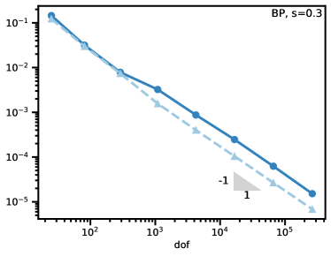
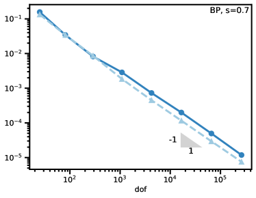
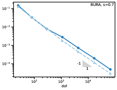
Figure 4: Two-dimensional product of sines test case: the Bank–Weiser estimator $\eta^{\mathrm{bw}}_{\mathcal{Q}_{s}}$ in solid blue line is compared to the exact error in dashed light blue line for two different rational schemes and two different fractional powers.

9.1.1 Parametric problems discretization error

Since we know the analytical solutions to the parametric problems in this case, it is possible to compute the exact parametric discretization errors $e_{l}:=\lVert u_{l}-u_{l,1}\rVert_{L^{2}}$, for each $l\in\llbracket-M,N\rrbracket$. This allows us to investigate the consequences of using the same mesh for all the parametric problems. In fig. 5 we have plotted the exact parametric errors after five steps of (uniform) refinement. As we can notice, the same mesh leads to a wide range of parametric errors values. These errors are particularly low when the diffusion part of the parametric operator is dominant. When the reaction part begin to domine the mesh seems to have a constant impact on the parametric errors (this is particularly striking for the BP scheme).

As expected these results suggest that the method can be optimized by using different meshes depending on $l$. In particular, coarser meshes would be sufficient when the diffusion coefficient is dominant. These results are obtained for mesh uniform refinement, further investigations deserve to be carried out for mesh adaptive refinement.

As we explained earlier, using a different hierarchy of meshes for each parametric problem may be computationally advantageous, at the expense of ease of implementation. Several hierarchies of meshes would need to be stored and, in the case of adaptive mesh refinement, interpolation between possibly non-nested meshes would be required in order to compute the fractional solution $u$. To avoid these complications when mesh adaptive refinement is used, we propose the following:

1. use the same hierarchy of meshes for all the parametric problems but not the same mesh. Some parametric problems might be solved on coarser meshes from the hierarchy and others on finer ones. This would allow to keep only one hierarchy of meshes stored in memory. Moreover, it would avoid the interpolation between non-nested meshes, since meshes from the same hierarchy are always nested.

2. selectively refine the mesh hierarchy: estimate the error globally for each parametric problem (this can be done using the local parametric Bank–Weiser solutions) and mark the parametric problems for which a finer mesh is required, using e.g. a marking algorithm similar to Dörfler’s marking strategy.

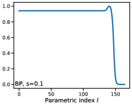
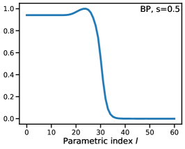
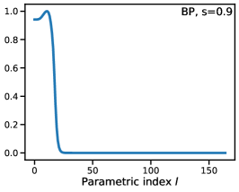
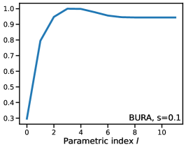
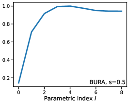
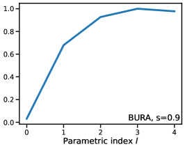
Figure 5: Two-dimensional product of sines text case: variation of the normalized exact parametric errors $e_{l}/\max_{l}(e_{l})$ with respect to the index $l\in\llbracket-M,N\rrbracket$ for BP and BURA and for three different fractional powers.

9.2 Two-dimensional checkerboard test case

We solve the problem introduced in the numerical results of [30]. We consider a unit square $\Omega=(0,1)^{2}$ with data $f:\Omega\to\mathbb{R}$ given for all $(x_{1},x_{2})\in\Omega$ by

$$f(x_{1},x_{2})=\begin{cases}1,&\text{if }(x_{1}-0.5)(x_{2}-0.5)>0,\\ -1,&\text{otherwise}.\end{cases}$$ (53)

The data $f$ belongs to $\mathbb{H}^{1/2-\varepsilon}(\Omega)$ for all $\varepsilon>0$. So in Theorem 4.3 of [30] the index $\delta<1/2$ and since $\Omega$ is convex, again $\alpha$ can be chosen equal to $1$. Then, the predicted convergence rate (for uniform refinement) is $\ln(\sqrt{\mathrm{dof}})\mathrm{dof}^{-\beta}$ with

$$\beta=\begin{cases}1,&\text{if }s>\tfrac{3}{4},\\ s+\tfrac{1}{4},&\text{otherwise}.\end{cases}$$ (54)

The predicted (if we omit the logarithmic term) and calculated convergence rates for different choices of $s$ are given in table 3. We recall that, to our knowledge, Theorem 4.3 is only available for BP and for BURA. As we can see on this table, the convergence rates for the total estimator is globally coherent with the predictions. Tables 3 and 6 show that mesh adaptive refinement improves the convergence rate for small fractional powers. This is expected, the deterioration in the convergence rate is due to the boundary layer behavior of the solution that is getting stronger as the fractional power decreases. In the limit as the fractional power approaches $s\to 1$, the solution behaves like the solution to a non-fractional problem, i.e. there is no boundary layer and mesh adaptive refinement is no longer needed to improve the convergence rate. Nevertheless, it appears that our estimation strategy deals properly with this limit case in terms of recovering the expected convergence rates for all $s$. This behavior can be seen on fig. 7, after 10 steps of mesh adaptive refinement, the mesh associated to fractional power $s=0.9$ is almost uniformly refined while the meshes associated to $s=0.5$ and $s=0.1$ show strongly localized refinement. This explains why in fig. 6 we see the expected behavior, i.e. no improvement in the convergence rate, when the mesh is adaptively refined compared to uniformly refined when $s\geqslant 0.7$.

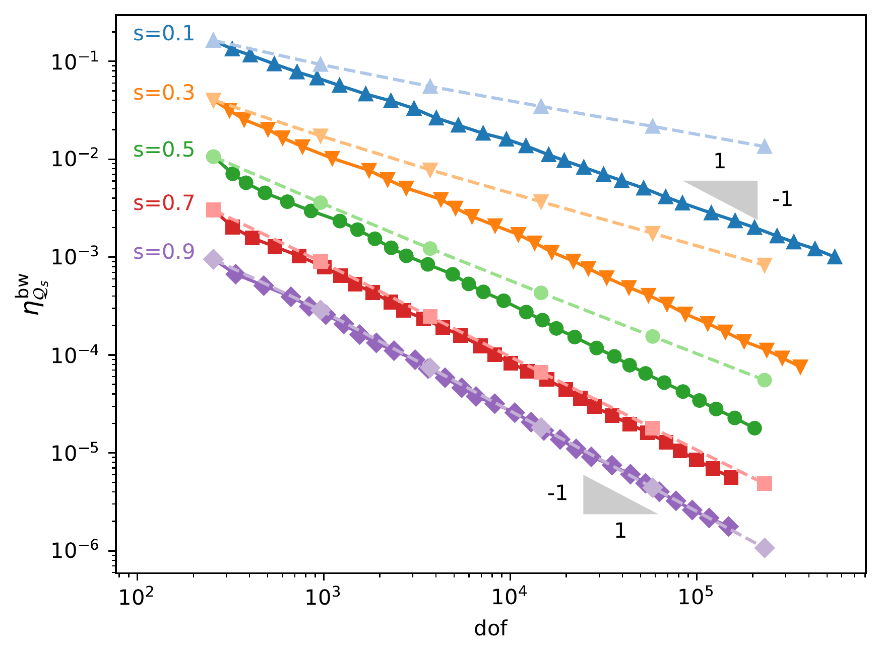
Figure 6: Two-dimensional checkerboard test case: the dashed lines represent the Bank–Weiser estimator when uniform mesh refinement is performed and the solid lines represent the estimator when adaptive mesh refinement is performed.

	Frac. power	0.1	0.3	0.5	0.7	0.9
BP	Theory [30]	-0.35	-0.55	-0.75	-0.95	-1.00
	Unif. mesh ref.	-0.35	-0.56	-0.77	-0.94	-1.00
	Adapt. mesh ref.	-0.66	-0.85	-0.95	-0.96	-1.02
BURA	Unif. mesh ref.	-0.34	-0.59	-0.77	-0.94	-1.00
	Adapt. mesh ref.	-0.54	-0.89	-0.95	-0.96	-1.02

Table 3: Two-dimensional checkerboard test case: convergence rates of the Bank–Weiser estimator for uniform mesh refinement and adaptive mesh refinement and for BP and BURA methods. In the case of the BP method, the convergence rates are compared with the values predicted by [30] for various fractional powers.

Figure 7: Two-dimensional checkerboard test case: meshes obtained after 10 steps of mesh adaptive refinement steered by the Bank–Weiser estimator for $s=0.1,\ s=0.5$ and $s=0.9$ from left to right.

9.3 Three-dimensional product of sines test case

This test case is the three-dimensional equivalent of the last test case. We solve eq. 4 on the cube $\Omega=(0,\pi)^{3}$ with data $f(x,y,z)=(2/\pi)^{3/2}\sin(x)\sin(y)\sin(z)$. The analytical solution to this problem is given by $u(x,y,z)=3^{-s}(2/\pi)^{3/2}\sin(x)\sin(y)\sin(z)$. The problem is solved on a hierarchy of uniformly refined Cartesian (tetrahedral) meshes. As for the two-dimensional case, the solution $u$ shows no boundary layer behavior and mesh adaptive refinement is not required. For the same reasons as for the two-dimensional case, Theorem 4.3 from [30] predicts a convergence rate of $\mathrm{dof}^{-2/3}$ for the finite element scheme. fig. 8 shows the values of the Bank–Weiser estimator and of the exact error (computed from the knowledge of the analytical solution) for $s=0.3$ and $s=0.7$. As in the two-dimensional case, the efficiency indices are relatively robust with respect to the fractional powers. They are shown for various fractional powers in table 5 and are computed by taking the average of the indices from the three last meshes of the hierarchy. As we can see, the Bank–Weiser estimator efficiency indices for this three-dimensional case are not as good as in the two-dimensional case. We have already observed this behavior for non-fractional problems [37]. We can notice that the convergence rates, given in table 4, are coherent with the predictions of Theorem 4.3 from [30]. The convergence rates are computed from a linear regression on the values computed from the three last meshes of the hierarchy.

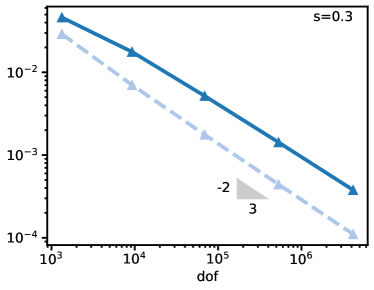
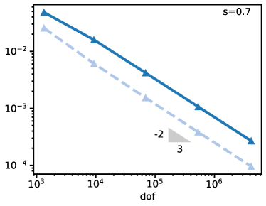
Figure 8: Three-dimensional product of sines test case: the Bank–Weiser estimator $\eta^{\mathrm{bw}}_{\mathcal{Q}_{s}}$ in solid dark blue line is compared to the exact error in dashed light blue line for $s=0.3$ and $s=0.7$ when the BP rational scheme is used.

Frac. power	0.1	0.3	0.5	0.7	0.9
Estimator	-0.56	-0.60	-0.63	-0.65	-0.66
Exact error	-0.69	-0.69	-0.69	-0.69	-0.69

Table 4: Three-dimensional product of sines test case: convergence rates of the Bank–Weiser estimator and of the exact error for various fractional powers when the BP rational scheme is used.

Frac. power	0.1	0.3	0.5	0.7	0.9
Est. eff. index	2.12	3.20	3.08	2.77	2.45

Table 5: Three-dimensional product of sines test case: efficiency indices of the Bank–Weiser estimator for various fractional powers.

9.4 Three-dimensional checkerboard test case

This test case is the three-dimensional version of the above checkerboard problem. We solve eq. 4 on the unit cube $\Omega=(0,1)^{3}$, with data $f$ such that

$$f(x_{1},x_{2},x_{3})=\begin{cases}1,&\text{if }(x_{1}-0.5)(x_{2}-0.5)>0\text{ and }(x_{3}-0.5)<0,\\ 1,&\text{if }(x_{1}-0.5)(x_{2}-0.5)<0\text{ and }(x_{3}-0.5)>0,\\ -1,&\text{otherwise.}\end{cases}$$ (55)

The finite element solution $u_{1}$ and the corresponding mesh after six steps of mesh adaptive refinement are shown in fig. 9 for the fractional power $s=0.5$. As for the two-dimensional case, $f\in\mathbb{H}^{1/2-\varepsilon}(\Omega)$ for all $\varepsilon>0$. Consequently, once again Theorem 4.3 of [30] predicts a convergence rate (for uniform refinement) equal to $\ln\left(\mathrm{dof}^{1/3}\right)\mathrm{dof}^{-2\beta/3}$ with $\beta$ given by eq. 54.

Once again, if we omit the logarithmic term, the predicted and calculated convergence rates are given in table 6. As in the two-dimensional case, the convergence rates of the Bank–Weiser estimator are globally coherent with the predictions and the boundary layer behavior becomes stronger as the fractional power decreases leading to poorer convergence rates. fig. 10 shows the values of the Bank–Weiser estimator for mesh uniform and adaptive refinement and for several fractional powers.

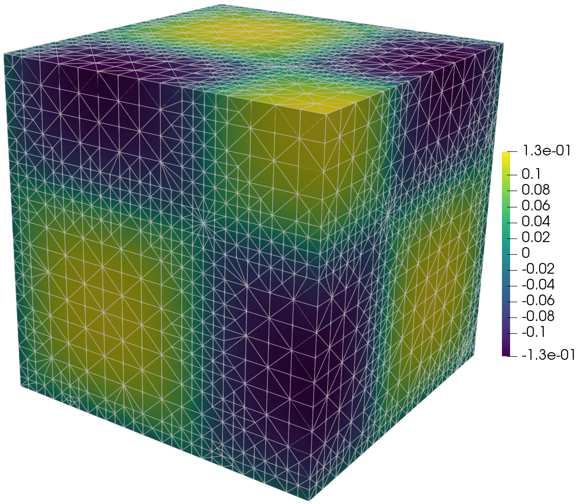
Figure 9: Three-dimensional checkerboard test case: finite element solution and mesh after six steps of mesh adaptive refinement when $s=0.5$. The unit cube domain $(0,1)^{3}$ is truncated by the three planes passing through the point $(0.25,0.25,0.25)$ and orthogonal to the vectors $(1,0,0)$, $(0,1,0)$ and $(0,0,1)$ respectively.

Frac. power	0.1	0.3	0.5	0.7	0.9
Theory [30]	-0.23	-0.37	-0.50	-0.63	-0.67
Unif. mesh ref.	-0.24	-0.38	-0.52	-0.62	-0.67
Adapt. mesh ref.	-0.33	-0.46	-0.55	-0.65	-0.68

Table 6: Three-dimensional checkerboard test case: convergence rates of the Bank–Weiser estimator for mesh uniform refinement and for mesh adaptive refinement compared to the values predicted by [30] for various fractional powers when the BP rational scheme is used.

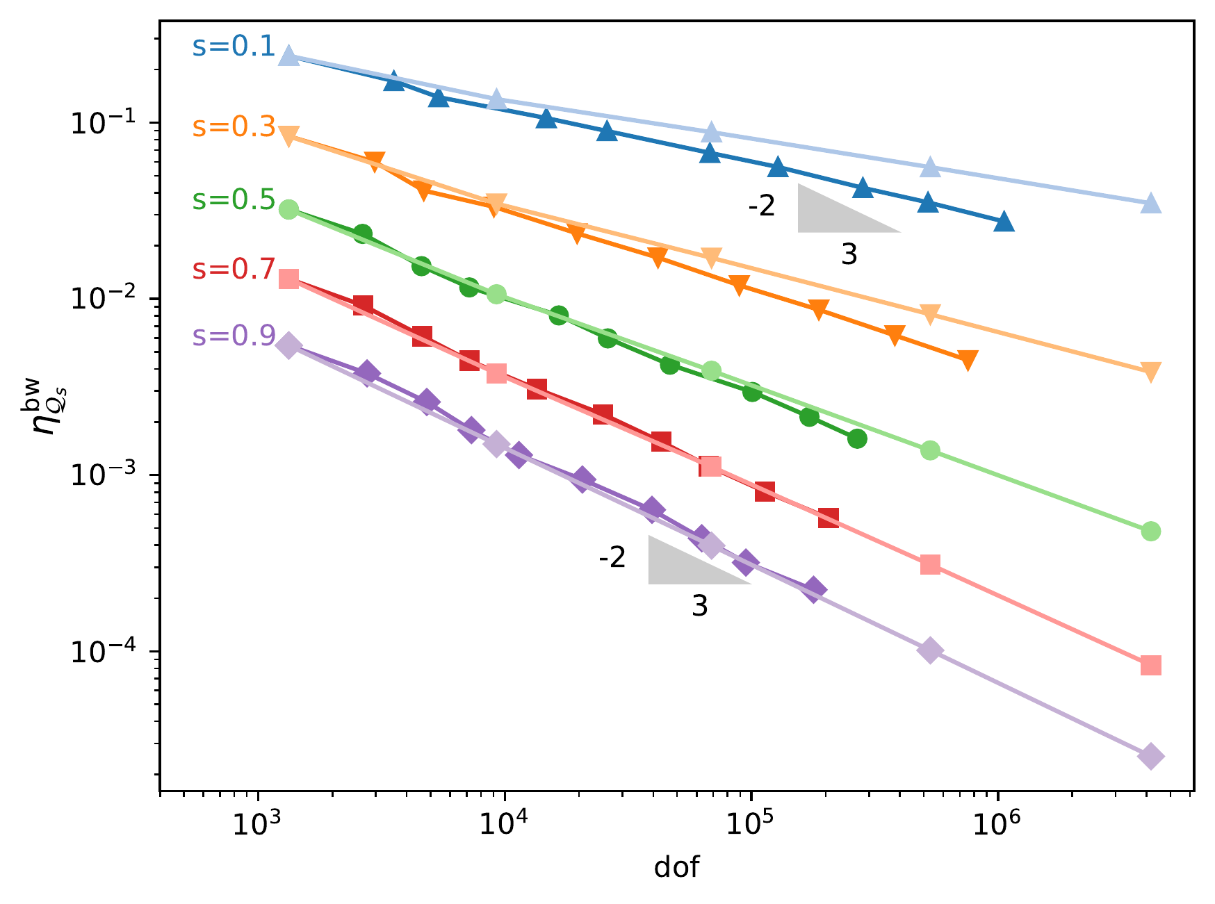
Figure 10: Three-dimensional checkerboard test case: for each fractional power we compare the values of the Bank–Weiser estimator $\eta^{\mathrm{bw}}_{\mathcal{Q}_{s}}$ when uniform refinement is performed (light lines) and when adaptive refinement is performed (darker lines).

9.5 Three–dimensional torus test case

We show now the application of our method on an unstructured three-dimensional mesh. We generate a mesh of a filled torus with unit inner radius and outer radius of $1.3$ using gmsh [66]. The initial mesh has 12040 tetrahedral cells. We set $s=0.5$ and $f=1$ for all $\Omega$. We estimate the lowest eigenvalue of the standard Laplacian on this mesh $\lambda_{0}\simeq 60$ and calculate of the data $\lVert f\rVert_{L^{2}}\simeq 1.323$ giving a quadrature fineness parameter $\kappa=0.48$ for the BP scheme (45 quadrature points).

We perform adaptive mesh refinement until a discretization error of less than $1\times 10^{-2}$ has been reached. The evolution of the estimator is given in fig. 11. A plot of the solution and an idea of the mesh refinement on a cut at the third and final mesh is given in fig. 12. Clearly evident is the very strong refinement near the boundary needed to capture the strong boundary layer in this problem.

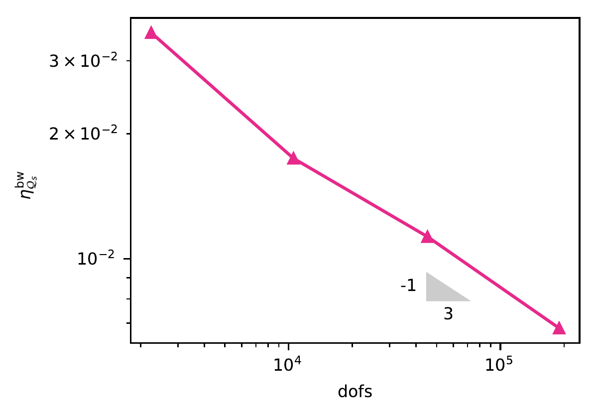
Figure 11: Three–dimensional torus test case: convergence of estimator under adaptive mesh refinement.

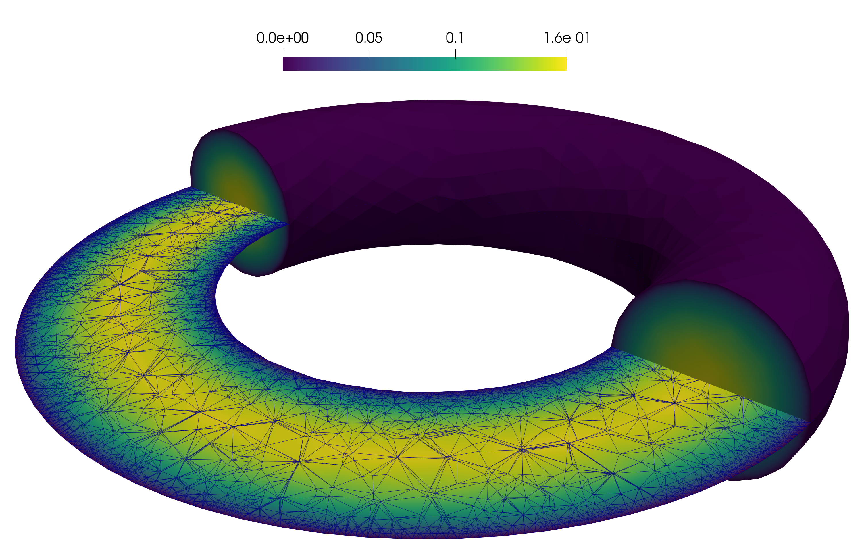
Figure 12: Three–dimensional torus test case: Plot of solution after the final mesh adaptive refinement. Clipped with plane passing through origin with normal $(1,0,0)$. Sliced with plane passing through origin with normal $(0,0,1)$. Slice shows mesh refinement with particularly strong refinement to resolve the boundary layer.

9.6 Adaptive rational scheme

In this section, we apply our method combining finite element mesh and rational scheme adaptive refinement (sketched in fig. 3) to the two-dimensional test cases from sections 9.2 and 9.1. We provide a comparison between this method and the method where the rational schemes are fixed. When an adaptive rational scheme is used the number of parametric problems is variable from one step to another. Thus, in order to obtain a meaningful comparison, we use the total number of degrees of freedom (i.e. the number of degrees of freedom times the number of parametric problems) on the plots x–axis. In addition, the rational approximation error is no longer negligible so our interest is on the total error estimator and the total discretization error (respectively defined in eq. 52 and eq. 26) rather than the Bank–Weiser estimator and the finite element discretization error.

9.6.1 Two-dimensional product of sines test case

In fig. 13 we compare the values of the total estimator $\eta$ and of the exact error with and without the use of an adaptive rational scheme. As in section 9.1, adaptive mesh refinement is not required on this test case so we only perform uniform mesh refinement.

In table 7 we compare the number of parametric problems solved with or without the use of an adaptive rational scheme. The total numbers of parametric problems to solve in order to reach our tolerance is reduced by 30 to 43 % for the BP method and by 40 to 48 % for the BURA method. However, and more surprisingly, the use of an adaptive rational scheme does not induce any gain in the overall computational cost –measured by the number of degrees of freedom times the number of parametric problems– for this test case, as we can see in fig. 13. We notice that the introduction of the adaptive rational scheme slightly deteriorate the convergence rates, shown in table 8. Our method consists in reducing the convergence rate of the rational approximation to the convergence rate of the Bank–Weiser estimator. Thus, it assumes that the rational scheme does not influence the Bank–Weiser estimator rate of convergence. However, the results in table 8 suggest that the Bank–Weiser estimator is influenced by the rational approximation scheme.

	Frac. power	0.1	0.3	0.5	0.7	0.9
BP	Fixed ra. scheme	1155	497	427	497	1155
	Adaptive ra. scheme	504	209	178	199	358
BURA	Fixed ra. scheme	96	77	63	49	35
	Adaptive ra. scheme	42	33	29	20	17

Table 7: Two-dimensional product of sines test case: comparison of the total number of solves to reach the tolerance for each method and each fractional power with and without the adaptively refined rational scheme.

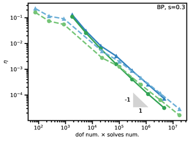
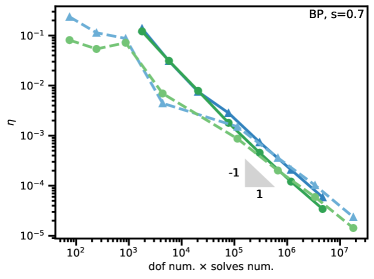
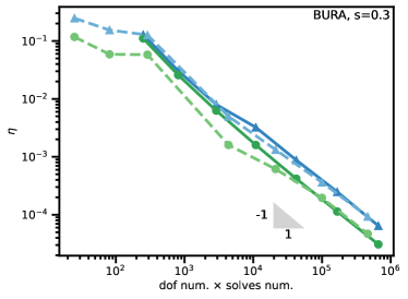
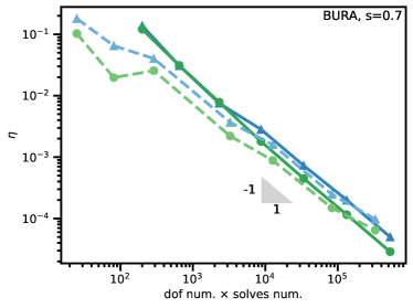
Figure 13: Two-dimensional product of sines test case: the solid lines represent fixed BP and BURA schemes while the dashed lines represent adaptive BP and BURA schemes. Triangular markers represent the values of the total estimator and circular markers represent the values of the exact total error.

		Frac. power	0.1	0.3	0.5	0.7	0.9
BP	Fixed scheme	Exact error	-1.03	-1.03	-1.04	-1.04	-1.04
		Estimator	-0.92	-0.93	-0.95	-0.96	-0.97
	Adaptive scheme	Exact error	-0.83	-0.75	-0.77	-0.73	-0.74
		Estimator	-0.78	-0.74	-0.83	-0.74	-0.77
BURA	Fixed scheme	Exact error	-0.80	-1.03	-1.05	-1.06	-1.06
		Estimator	-0.78	-0.94	-0.96	-0.98	-0.99
	Adaptive scheme	Exact error	-0.67	-0.83	-0.84	-0.77	-0.77
		Estimator	-0.71	-0.85	-0.83	-0.80	-0.79

Table 8: Two-dimensional product of sines test case: convergence rates of the total estimator and of the exact total error for various fractional powers and for fixed or adaptive BP and BURA schemes.

	Frac. power	0.1	0.3	0.5	0.7	0.9
BP	Fixed scheme	1.76	2.03	1.79	1.52	1.29
	Adaptive scheme	1.69	1.75	1.73	1.51	1.85
BURA	Fixed scheme	1.02	1.93	1.81	1.53	1.30
	Adaptive scheme	1.44	2.25	2.00	1.64	2.07

Table 9: Two-dimensional product of sines test case: efficiency indices of the total estimator for various fractional powers and for fixed or adaptive BP and BURA schemes.

9.6.2 Two-dimensional checkerboard test case

In fig. 14 we compare the values of the total estimator $\eta$ and of the exact error with and without the use of an adaptive rational scheme. As in section 9.2, the boundary layer behavior, present for small values of $s$, requires adaptive mesh refinement but gets less and less prominent as $s$ tends to 1.

The gain in the number of parametric problems to solve is comparable to what we obtain in table 7. The use of an adaptive rational scheme clearly induces a gain in the precision with respect to the total number of degrees of freedom, except for small fractional powers when the BURA rational scheme is used.

As for the two–dimensional product of sines test case, we can notice on table 10 that the use of an adaptive rational scheme also deteriorates the convergence rates in most of the cases. However, unlike the test case from section 9.6.1, a gain in the computational cost clearly appears when an adaptive rational scheme is used, especially with the BP method.

The discrepancies between the BP and BURA methods might be due to the high sensitivity of the BURA scheme with respect to the parameter $N$: balancing the rational and finite element estimator is more difficult with the BURA scheme.

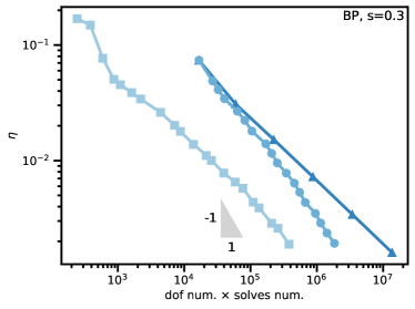
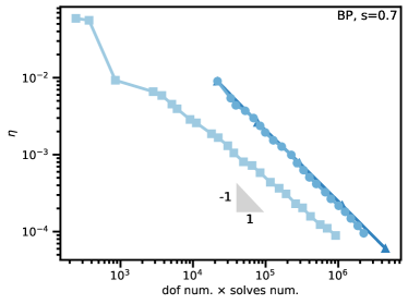
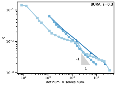
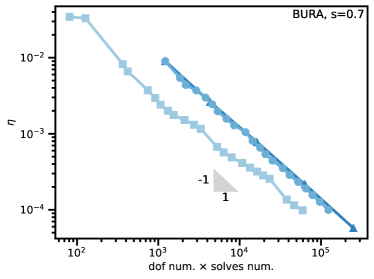
Figure 14: Two-dimensional checkerboard test case: we compare the values of the total estimator for three refinement strategies, when the mesh is uniformly refined and a fixed rational scheme is used (triangular markers), when the mesh is adaptively refined and a fixed rational scheme is used (circular markers) and when the mesh is adaptively refined and an adaptive rational scheme is used (square markers).

	Frac. power	0.1	0.3	0.5	0.7	0.9
BP	Theory [30]	-0.35	-0.55	-0.75	-0.95	-1.00
	Unif. mesh ref.	-0.35	-0.56	-0.77	-0.94	-1.00
	Adapt. mesh ref.	-0.57	-0.77	-0.94	-0.97	-1.00
	Adapt. mesh ref. & ra. sch.	-0.44	-0.56	-0.75	-0.78	-0.82
BURA	Unif. mesh ref.	-0.21	-0.65	-0.83	-0.94	-1.00
	Adapt. mesh ref.	-0.36	-0.79	-0.97	-0.96	-1.00
	Adapt. mesh ref. & ra. sch.	-0.45	-0.50	-0.65	-0.80	-0.86

Table 10: Two-dimensional checkerboard test case: convergence rates of the total estimator for uniform mesh refinement, adaptive mesh refinement and adaptive mesh refinement combined with rational scheme adaptation respectively for BP and BURA methods. The convergence rates are compared with the values predicted by [30] (in the case of uniform refinement) for various fractional powers.

10 Concluding remarks

In this work we presented a novel a posteriori error estimation method for the spectral fractional Laplacian. This method benefits from the parallel character of both the Bank–Weiser error estimator and the rational approximation methods, thus keeping the appealing computational aspects of the underlying methodology in [30]. Here are some important points we want to make to conclude this paper. First, the Bank–Weiser estimator seems to be equivalent to the $L^{2}$ exact error at least when structured meshes are used and when the solution $u$ is smooth. Second, adaptive mesh refinement methods drastically improves the convergence rate compared to uniform refinement for fractional powers close to $0$. Third, the use of an adaptive rational scheme can reduce the number of total parametric problems to solve by $30$ to $48\%$ depending on the scheme and the fractional power. However, it does not necessarily induce a gain in the precision with respect to the total number of degrees of freedom.

Finally, we give some future directions that we think are worth considering. More numerical tests could be performed, especially for higher order elements and/or using variants of the Bank–Weiser error estimator as considered in [39].

We would like also to study the derivation of an algorithm that allows to use different meshes to discretize the parametric problems in order to save computational time, as explained in section 9.1.1. However, the implementation of this strategy requires to interpolate functions between different meshes, which is not currently available in the FEniCSx software and by consequence, is beyond the scope of this study. The use of an adaptive rational scheme and in particular the dependence of the Bank–Weiser estimator with respect to the choice of the rational scheme deserve a deeper investigation in order to fully explain the results in sections 9.6.1 and 9.6.2. The a posteriori error estimation of the error in the “natural” norm of the problem i.e. the spectral fractional norm defined in eq. 3 is another extension of this work that is worth to consider. The replacement of the Bank–Weiser estimator by an anisotropic a posteriori error estimator would improve the convergence rate even further in case of boundary layers, see e.g. [19, 62], Another interesting extension would be to test our method on fractional powers of other kinds of elliptic operators, following [30], on another definition of the fractional Laplacian operator [27] and/or other boundary conditions, following [15].

Supplementary material

A minimal example of adaptive finite element method for the two–dimensional spectral fractional Laplacian and the three–dimensional torus can be found in the following FEniCSx–Error–Estimation repository https://github.com/jhale/fenicsx-error-estimation. This minimal example code (LGPLv3) is also archived at https://doi.org/10.6084/m9.figshare.19086695.v3. A Docker image [70] is provided in which this code can be executed.

References

- [1] Lidia Aceto, Daniele Bertaccini, Fabio Durastante, and Paolo Novati. Rational Krylov methods for functions of matrices with applications to fractional partial differential equations. J. Comput. Phys., 396:470–482, nov 2019. doi:10.1016/j.jcp.2019.07.009.
- [2] Lidia Aceto and Paolo Novati. Rational Approximation to the Fractional Laplacian Operator in Reaction-Diffusion Problems. SIAM J. Sci. Comput., 39(1):A214–A228, jan 2017. arXiv:1607.04166, doi:10.1137/16M1064714.
- [3] Lidia Aceto and Paolo Novati. Rational approximations to fractional powers of self-adjoint positive operators. Numer. Math., 143(1):1–16, sep 2019. arXiv:1807.10086, doi:10.1007/s00211-019-01048-4.
- [4] Gabriel Acosta, Francisco M Bersetche, and Juan Pablo Borthagaray. A short FE implementation for a 2d homogeneous Dirichlet problem of a fractional Laplacian. Comput. Math. with Appl., 74(4):784–816, aug 2017. arXiv:1610.05558, doi:10.1016/j.camwa.2017.05.026.
- [5] Gabriel Acosta and Juan Pablo Borthagaray. A Fractional Laplace Equation: Regularity of Solutions and Finite Element Approximations. SIAM J. Numer. Anal., 55(2):472–495, jan 2017. arXiv:1507.08970, doi:10.1137/15M1033952.
- [6] Mark Ainsworth and Christian Glusa. Aspects of an adaptive finite element method for the fractional Laplacian: A priori and a posteriori error estimates, efficient implementation and multigrid solver. Comput. Methods Appl. Mech. Eng., 327:4–35, dec 2017. arXiv:1708.03912, doi:10.1016/j.cma.2017.08.019.
- [7] Mark Ainsworth and Christian Glusa. Hybrid Finite Element–Spectral Method for the Fractional Laplacian: Approximation Theory and Efficient Solver. SIAM J. Sci. Comput., 40(4):A2383–A2405, jan 2018. URL: https://epubs.siam.org/doi/10.1137/17M1144696, arXiv:1709.01639, doi:10.1137/17M1144696.
- [8] Mark Ainsworth and Christian Glusa. Towards an Efficient Finite Element Method for the Integral Fractional Laplacian on Polygonal Domains. Contemp. Comput. Math. - A Celebr. 80th Birthd. Ian Sloan, 40:17–57, 2018. arXiv:1708.01923, doi:10.1007/978-3-319-72456-0_2.
- [9] Mark Ainsworth and Zhiping Mao. Analysis and Approximation of a Fractional Cahn–Hilliard Equation. SIAM J. Numer. Anal., 55(4):1689–1718, jan 2017. doi:10.1137/16M1075302.
- [10] Mark Ainsworth and J Tinsley Oden. A Posteriori Error Estimation in Finite Element Analysis. Pure and Applied Mathematics (New York). John Wiley & Sons, Inc., Hoboken, NJ, USA, aug 2000. doi:10.1002/9781118032824.
- [11] Goro Akagi, Giulio Schimperna, and Antonio Segatti. Fractional Cahn–Hilliard, Allen–Cahn and porous medium equations. J. Differ. Equ., 261(6):2935–2985, sep 2016. arXiv:1502.06383, doi:10.1016/j.jde.2016.05.016.
- [12] Grégoire Allaire. Numerical analysis and optimization: an introduction to mathematical modelling and numerical simulation. Numerical mathematics and scientific computation. Oxford University Press, Oxford ; New York, 2007. OCLC: ocm82671667.
- [13] Martin S Alnæs, Jan Blechta, Johan Hake, August Johansson, Benjamin Kehlet, Anders Logg, Chris Richardson, Johannes Ring, Marie E Rognes, and Garth N Wells. The FEniCS Project Version 1.5. Arch. Numer. Softw., 2015. doi:10.11588/ans.2015.100.20553.
- [14] Harbir Antil and Enrique Otárola. A FEM for an Optimal Control Problem of Fractional Powers of Elliptic Operators. SIAM J. Control Optim., 53(6):3432–3456, jan 2015. arXiv:1406.7460, doi:10.1137/140975061.
- [15] Harbir Antil, Johannes Pfefferer, and Sergejs Rogovs. Fractional operators with inhomogeneous boundary conditions: analysis, control, and discretization. Commun. Math. Sci., 16(5):1395–1426, 2018. arXiv:1703.05256, doi:10.4310/CMS.2018.v16.n5.a11.
- [16] Abdon Atangana. Fractional Operators and Their Applications. In Fract. Oper. with Constant Var. Order with Appl. to Geo-Hydrology, pages 79–112. Elsevier, 2018. doi:10.1016/B978-0-12-809670-3.00005-9.
- [17] Alampallam V Balakrishnan. Fractional powers of closed operators and the semigroups generated by them. Pacific J. Math., 10(2):419–437, jun 1960. doi:10.2140/pjm.1960.10.419.
- [18] Satish Balay, Shrirang Abhyankar, Mark F Adams, Jed Brown, Peter Brune, Kris Buschelman, Lisandro Dalcin, Victor Eijkhout, William D Gropp, Dinesh Kaushik, Matthew G Knepley, Lois Curfman McInnes, Karl Rupp, Barry F Smith, Stefano Zampini, Hong Zhang, and Hong Zhang. PETSc Users Manual. Technical Report ANL-95/11 - Revision 3.7, Argonne National Laboratory, 2016. URL: http://www.mcs.anl.gov/petsc.
- [19] Lehel Banjai, Jens M Melenk, Ricardo H Nochetto, Enrique Otárola, Abner J Salgado, and Christoph Schwab. Tensor FEM for Spectral Fractional Diffusion. Found. Comput. Math., 19(4):901–962, aug 2019. arXiv:1707.07367, doi:10.1007/s10208-018-9402-3.
- [20] Lehel Banjai, Jens M Melenk, and Christoph Schwab. Exponential convergence of hp FEM for spectral fractional diffusion in polygons. arXiv, pages 1–37, 2020. arXiv:2011.05701.
- [21] Randolph E Bank and Alan Weiser. Some A Posteriori Error Estimators for Elliptic Partial Differential Equations. Math. Comput., 44(170):283, apr 1985. doi:10.2307/2007953.
- [22] O Barrera. A unified modelling and simulation for coupled anomalous transport in porous media and its finite element implementation. Computational Mechanics, pages 1–16, 2021.
- [23] David Bolin, Kristin Kirchner, and Mihály Kovács. Numerical solution of fractional elliptic stochastic PDEs with spatial white noise. IMA J. Numer. Anal., 40(2):1051–1073, apr 2020. arXiv:1705.06565, doi:10.1093/imanum/dry091.
- [24] Andrea Bonito, Juan Pablo Borthagaray, Ricardo H Nochetto, Enrique Otárola, and Abner J Salgado. Numerical methods for fractional diffusion. Comput. Vis. Sci., 19(5-6):19–46, dec 2018. arXiv:1707.01566, doi:10.1007/s00791-018-0289-y.
- [25] Andrea Bonito, Wenyu Lei, and Joseph E Pasciak. Numerical Approximation of Space-Time Fractional Parabolic Equations. Comput. Methods Appl. Math., 17(4):679–705, oct 2017. arXiv:1704.04254, doi:10.1515/cmam-2017-0032.
- [26] Andrea Bonito, Wenyu Lei, and Joseph E Pasciak. The approximation of parabolic equations involving fractional powers of elliptic operators. J. Comput. Appl. Math., 315:32–48, may 2017. arXiv:1607.07832, doi:10.1016/j.cam.2016.10.016.
- [27] Andrea Bonito, Wenyu Lei, and Joseph E Pasciak. Numerical approximation of the integral fractional Laplacian. Numer. Math., 142(2):235–278, jun 2019. arXiv:1707.04290, doi:10.1007/s00211-019-01025-x.
- [28] Andrea Bonito, Wenyu Lei, and Joseph E Pasciak. On sinc quadrature approximations of fractional powers of regularly accretive operators. J. Numer. Math., 27(2):57–68, jun 2019. arXiv:1709.06619, doi:10.1515/jnma-2017-0116.
- [29] Andrea Bonito and Murtazo Nazarov. Numerical Simulations of Surface Quasi-Geostrophic Flows on Periodic Domains. SIAM J. Sci. Comput., 43(2):B405–B430, jan 2021. arXiv:2006.01180, doi:10.1137/20M1342616.
- [30] Andrea Bonito and Joseph E Pasciak. Numerical approximation of fractional powers of elliptic operators. Math. Comput., 84(295):2083–2110, mar 2015. arXiv:1307.0888, doi:10.1090/S0025-5718-2015-02937-8.
- [31] Andrea Bonito and Joseph E Pasciak. Numerical approximation of fractional powers of regularly accretive operators. IMA J. Numer. Anal., page drw042, aug 2016. arXiv:1508.05869, doi:10.1093/imanum/drw042.
- [32] Andrea Bonito and Peng Wei. Electroconvection of thin liquid crystals: Model reduction and numerical simulations. J. Comput. Phys., 405:109140, mar 2020. doi:10.1016/j.jcp.2019.109140.
- [33] Stéphane P.A. Bordas, Sundararajan Natarajan, and Alexander Menk. Partition of unity methods. Wiley-blackwell edition, 2016.
- [34] Juan Borthagaray, Wenbo Li, and Ricardo H Nochetto. Linear and nonlinear fractional elliptic problems. pages 69–92, jun 2020. arXiv:1906.04230, doi:10.1090/conm/754/15145.
- [35] Juan Pablo Borthagaray, Dmitriy Leykekhman, and Ricardo H Nochetto. Local Energy Estimates for the Fractional Laplacian. SIAM J. Numer. Anal., 59(4):1918–1947, jan 2021. arXiv:2005.03786, doi:10.1137/20M1335509.
- [36] Raphaël Bulle, Gioacchino Alotta, Gregorio Marchiori, Matteo Berni, Nicola F. Lopomo, Stefano Zaffagnini, Stéphane P. A. Bordas, and Olga Barrera. The Human Meniscus Behaves as a Functionally Graded Fractional Porous Medium under Confined Compression Conditions. Appl. Sci., 11(20):9405, oct 2021. doi:10.3390/app11209405.
- [37] Raphaël Bulle, Franz Chouly, Jack S Hale, and Alexei Lozinski. Removing the saturation assumption in Bank–Weiser error estimator analysis in dimension three. Appl. Math. Lett., 107:106429, sep 2020. doi:10.1016/j.aml.2020.106429.
- [38] Raphaël Bulle and Jack S Hale. FEniCS Error Estimation (FEniCS-EE), jan 2019. doi:10.6084/m9.figshare.10732421.
- [39] Raphaël Bulle, Jack S. Hale, Alexei Lozinski, Stéphane P.A. Bordas, and Franz Chouly. Hierarchical a posteriori error estimation of Bank–Weiser type in the FEniCS Project. Computers & Mathematics with Applications, 131:103–123, February 2023. URL: https://linkinghub.elsevier.com/retrieve/pii/S0898122122004722, doi:10.1016/j.camwa.2022.11.009.
- [40] Luis Caffarelli and Luis Silvestre. An Extension Problem Related to the Fractional Laplacian. Commun. Partial Differ. Equations, 32(8):1245–1260, aug 2007. arXiv:0608640, doi:10.1080/03605300600987306.
- [41] Eric Cancès, Geneviève Dusson, Yvon Maday, Benjamin Stamm, and Martin Vohralík. Guaranteed and Robust a Posteriori Bounds for Laplace Eigenvalues and Eigenvectors: Conforming Approximations. SIAM J. Numer. Anal., 55(5):2228–2254, jan 2017. doi:10.1137/15M1038633.
- [42] Michele Caputo. Linear Models of Dissipation whose Q is almost Frequency Independent–II. Geophys. J. Int., 13(5):529–539, nov 1967. doi:10.1111/j.1365-246X.1967.tb02303.x.
- [43] Michele Caputo. Models of flux in porous media with memory. Water Resour. Res., 36(3):693–705, mar 2000. doi:10.1029/1999WR900299.
- [44] Max Carlson, Robert M Kirby, and Hari Sundar. A scalable framework for solving fractional diffusion equations. Proc. 34th ACM Int. Conf. Supercomput., pages 1–11, jun 2020. arXiv:1911.11906, doi:10.1145/3392717.3392769.
- [45] Carsten Carstensen and Joscha Gedicke. Guaranteed lower bounds for eigenvalues. Math. Comput., 83(290):2605–2629, apr 2014. doi:10.1090/S0025-5718-2014-02833-0.
- [46] Carsten Carstensen and Christian Merdon. Estimator Competition for poisson Problems. J. Comput. Math., 28(3):309–330, 2010. doi:10.4208/jcm.2009.10-m1010.
- [47] Huyuan Chen. The Dirichlet elliptic problem involving regional fractional Laplacian. J. Math. Phys., 59(7):071504, jul 2018. arXiv:1509.05838, doi:10.1063/1.5046685.
- [48] Long Chen, Ricardo H Nochetto, Enrique Otárola, and Abner J Salgado. A PDE approach to fractional diffusion: A posteriori error analysis. J. Comput. Phys., 293:339–358, jul 2015. doi:10.1016/j.jcp.2015.01.001.
- [49] Nathan Collier, Abdul-Lateef Haji-Ali, Fabio Nobile, Erik von Schwerin, and Raúl Tempone. A continuation multilevel Monte Carlo algorithm. BIT Numerical Mathematics, 55(2):399–432, June 2015. URL: http://link.springer.com/10.1007/s10543-014-0511-3, doi:10.1007/s10543-014-0511-3.
- [50] Nicole Cusimano, Félix del Teso, and Luca Gerardo-Giorda. Numerical approximations for fractional elliptic equations via the method of semigroups. ESAIM Math. Model. Numer. Anal., 54(3):751–774, may 2020. doi:10.1051/m2an/2019076.
- [51] Nicole Cusimano, Félix del Teso, Luca Gerardo-Giorda, and Gianni Pagnini. Discretizations of the Spectral Fractional Laplacian on General Domains with Dirichlet, Neumann, and Robin Boundary Conditions. SIAM J. Numer. Anal., pages 1243–1272, jan 2018. arXiv:1708.03602, doi:10.1137/17M1128010.
- [52] Tobias Danczul and Joachim Schöberl. A Reduced Basis Method For Fractional Diffusion Operators I. pages 1–19, 2019. URL: http://arxiv.org/abs/1904.05599, arXiv:1904.05599.
- [53] Tobias Danczul and Joachim Schöberl. A reduced basis method for fractional diffusion operators II. J. Numer. Math., 29(4):269–287, oct 2021. arXiv:2005.03574, doi:10.1515/jnma-2020-0042.
- [54] Ozlem Defterli, Marta D’Elia, Qiang Du, Max Gunzburger, Rich Lehoucq, and Mark M Meerschaert. Fractional Diffusion on Bounded Domains. Fract. Calc. Appl. Anal., pages 1689–1699, jan 2015. arXiv:arXiv:1011.1669v3, doi:10.1515/fca-2015-0023.
- [55] Marta D’Elia and Max Gunzburger. The fractional Laplacian operator on bounded domains as a special case of the nonlocal diffusion operator. Comput. Math. with Appl., pages 1245–1260, oct 2013. arXiv:1303.6934, doi:10.1016/j.camwa.2013.07.022.
- [56] Huy Dinh, Harbir Antil, Yanlai Chen, Elena Cherkaev, and Akil Narayan. Model reduction for fractional elliptic problems using Kato’s formula. Math. Control Relat. Fields, 2021. doi:10.3934/mcrf.2021004.
- [57] Willy Dörfler. A Convergent Adaptive Algorithm for Poisson’s Equation. SIAM J. Numer. Anal., 33(3):1106–1124, jun 1996. doi:10.1137/0733054.
- [58] Qiang Du, Jiang Yang, and Zhi Zhou. Time-Fractional Allen–Cahn Equations: Analysis and Numerical Methods. J. Sci. Comput., page 42, nov 2020. arXiv:1906.06584, doi:10.1007/s10915-020-01351-5.
- [59] Siwei Duo, Hong Wang, and Yanzhi Zhang. A comparative study on nonlocal diffusion operators related to the fractional Laplacian. Discret. Contin. Dyn. Syst. - B, pages 231–256, 2019. arXiv:1711.06916, doi:10.3934/dcdsb.2018110.
- [60] Robert D Falgout and Ulrike Meier Yang. hypre: A Library of High Performance Preconditioners. In Peter M A Sloot, Alfons G Hoekstra, C J Kenneth Tan, and Jack J Dongarra, editors, Comput. Science — ICCS 2002, number 2331 in Lecture Notes in Computer Science, pages 632–641. Springer Berlin Heidelberg, apr 2002. doi:10.1007/3-540-47789-6_66.
- [61] Mouhamed M Fall. Regional fractional Laplacians: Boundary regularity. arXiv, jul 2020. URL: http://arxiv.org/abs/2007.04808, arXiv:2007.04808.
- [62] Markus Faustmann, Michael Karkulik, and Jens M Melenk. Local convergence of the FEM for the integral fractional Laplacian. arXiv, pages 1–20, may 2020. URL: http://arxiv.org/abs/2005.14109, arXiv:2005.14109.
- [63] Markus Faustmann, Jens M Melenk, and Dirk Praetorius. Quasi-optimal convergence rate for an adaptive method for the integral fractional Laplacian. Math. Comput., 90(330):1557–1587, apr 2021. arXiv:1903.10409, doi:10.1090/mcom/3603.
- [64] Ivan P Gavrilyuk, Wolfgang Hackbusch, and Boris N Khoromskij. Data-sparse approximation to the operator-valued functions of elliptic operator. Math. Comput., pages 1297–1325, jul 2003. doi:10.1090/S0025-5718-03-01590-4.
- [65] Ivan P Gavrilyuk, Wolfgang Hackbusch, and Boris N Khoromskij. Data-sparse approximation to a class of operator-valued functions. Math. Comput., pages 681–709, aug 2004. doi:10.1090/S0025-5718-04-01703-X.
- [66] Christophe Geuzaine and Jean-François Remacle. Gmsh: A 3-D finite element mesh generator with built-in pre- and post-processing facilities. International Journal for Numerical Methods in Engineering, 79(11):1309–1331, September 2009. URL: http://onlinelibrary.wiley.com/doi/10.1002/nme.2579/abstract, doi:10.1002/nme.2579.
- [67] Heiko Gimperlein and Jakub Stocek. Space–time adaptive finite elements for nonlocal parabolic variational inequalities. Comput. Methods Appl. Mech. Eng., pages 137–171, aug 2019. arXiv:1810.06888, doi:10.1016/j.cma.2019.04.019.
- [68] Gerd Grubb. Fractional Laplacians on domains, a development of Hörmander’s theory of -transmission pseudodifferential operators. Adv. Math. (N. Y)., 268:478–528, jan 2015. doi:10.1016/j.aim.2014.09.018.
- [69] Michal Habera, Jack S Hale, Chris Richardson, Johannes Ring, Marie Rognes, Nate Sime, and Garth N Wells. FEniCSX: A sustainable future for the FEniCS Project. 2020. doi:10.6084/m9.figshare.11866101.v1.
- [70] Jack S. Hale, Lizao Li, Christopher N. Richardson, and Garth N. Wells. Containers for Portable, Productive, and Performant Scientific Computing. Computing in Science & Engineering, 19(6):40–50, November 2017. doi:10.1109/MCSE.2017.2421459.
- [71] Stanislav Harizanov, Raytcho Lazarov, Svetozar Margenov, Pencho Marinov, and Yavor Vutov. Optimal solvers for linear systems with fractional powers of sparse SPD matrices. Numer. Linear Algebr. with Appl., 25(5):e2167, oct 2018. arXiv:1612.04846, doi:10.1002/nla.2167.
- [72] Stanislav Harizanov, Svetozar Margenov, and Nedyu Popivanov. Spectral Fractional Laplacian with Inhomogeneous Dirichlet Data: Questions, Problems, Solutions. pages 123–138, 2021. arXiv:arXiv:2010.01383v1, doi:10.1007/978-3-030-71616-5_13.
- [73] Nicholas J. Higham and Lijing Lin. An Improved Schur–Padé Algorithm for Fractional Powers of a Matrix and Their Fréchet Derivatives. SIAM J. Matrix Anal. Appl., 34(3):1341–1360, jan 2013. doi:10.1137/130906118.
- [74] Clemens Hofreither. A unified view of some numerical methods for fractional diffusion. Comput. Math. with Appl., 80(2):332–350, jul 2020. doi:10.1016/j.camwa.2019.07.025.
- [75] Clemens Hofreither. An algorithm for best rational approximation based on barycentric rational interpolation. Numer. Algorithms, 88(1):365–388, sep 2021. doi:10.1007/s11075-020-01042-0.
- [76] Mateusz Kwaśnicki. Ten equivalent definitions of the fractional laplace operator. Fract. Calc. Appl. Anal., 20(1):7–51, jan 2017. arXiv:1507.07356, doi:10.1515/fca-2017-0002.
- [77] Finn Lindgren, Håvard Rue, and Johan Lindström. An explicit link between Gaussian fields and Gaussian Markov random fields: the stochastic partial differential equation approach. J. R. Stat. Soc. Ser. B (Statistical Methodol.), 73(4):423–498, sep 2011. doi:10.1111/j.1467-9868.2011.00777.x.
- [78] Anna Lischke, Guofei Pang, Mamikon Gulian, Fangying Song, Christian Glusa, Xiaoning Zheng, Zhiping Mao, Wei Cai, Mark M Meerschaert, Mark Ainsworth, and George Em Karniadakis. What is the fractional Laplacian? A comparative review with new results. J. Comput. Phys., 404:109009, mar 2020. arXiv:1801.09767, doi:10.1016/j.jcp.2019.109009.
- [79] Dominik Meidner, Johannes Pfefferer, Klemens Schürholz, and Boris Vexler. -Finite Elements for Fractional Diffusion. SIAM J. Numer. Anal., 56(4):2345–2374, jan 2018. arXiv:1706.04066, doi:10.1137/17M1135517.
- [80] Chenchen Mou and Yingfei Yi. Interior Regularity for Regional Fractional Laplacian. Commun. Math. Phys., 340(1):233–251, nov 2015. doi:10.1007/s00220-015-2445-2.
- [81] Ricardo H Nochetto, Enrique Otárola, and Abner J Salgado. A PDE Approach to Fractional Diffusion in General Domains: A Priori Error Analysis. Found. Comput. Math., 15(3):733–791, jun 2015. arXiv:1302.0698, doi:10.1007/s10208-014-9208-x.
- [82] Ricardo H Nochetto, Tobias von Petersdorff, and Chen-Song Zhang. A posteriori error analysis for a class of integral equations and variational inequalities. Numer. Math., 116(3):519–552, sep 2010. doi:10.1007/s00211-010-0310-y.
- [83] Angel Plaza and Graham F Carey. Local refinement of simplicial grids based on the skeleton. Appl. Numer. Math., 32(2):195–218, feb 2000. doi:10.1016/S0168-9274(99)00022-7.
- [84] Igor Podlubny, Aleksei Chechkin, Tomas Skovranek, YangQuan Chen, and Blas M. Vinagre Jara. Matrix approach to discrete fractional calculus II: Partial fractional differential equations. J. Comput. Phys., 228(8):3137–3153, may 2009. doi:10.1016/j.jcp.2009.01.014.
- [85] Herbert R. Stahl. Best uniform rational approximation of on . Acta Mathematica, 190(2):241 – 306, 2003. doi:10.1007/BF02392691.
- [86] Pablo Raúl Stinga. User’s guide to the fractional Laplacian and the method of semigroups. In Fract. Differ. Equations, pages 235–266. De Gruyter, feb 2019. arXiv:1808.05159, doi:10.1515/9783110571660-012.
- [87] Pablo Raúl Stinga and José Luis Torrea. Extension Problem and Harnack’s Inequality for Some Fractional Operators. Commun. Partial Differ. Equations, 35(11):2092–2122, oct 2010. arXiv:0910.2569, doi:10.1080/03605301003735680.
- [88] Petr N Vabishchevich. Approximation of a fractional power of an elliptic operator. Numer. Linear Algebr. with Appl., 27(3):1–17, may 2020. arXiv:1905.10838, doi:10.1002/nla.2287.
- [89] Rüdiger Verfürth. Robust a posteriori error estimators for a singularly perturbed reaction-diffusion equation. Numer. Math., 78(3):479–493, jan 1998. doi:10.1007/s002110050322.
- [90] Christian J Weiss, Bart G van Bloemen Waanders, and Habir Antil. Fractional Operators Applied to Geophysical Electromagnetics. Geophys. J. Int., pages 1242–1259, nov 2019. arXiv:1902.05096, doi:10.1093/gji/ggz516.
- [91] Xuan Zhao, Xiaozhe Hu, Wei Cai, and George Em Karniadakis. Adaptive finite element method for fractional differential equations using hierarchical matrices. Comput. Methods Appl. Mech. Eng., 325:56–76, oct 2017. arXiv:1603.01358, doi:10.1016/j.cma.2017.06.017.