QED and strong isospin corrections in the hadronic vacuum polarization contribution to the anomalous magnetic moment of the muon

Abstract

Recently, the Budapest-Marseille-Wuppertal collaboration achieved sub-percent precision in the evaluation of the lowest-order hadronic vacuum polarization contribution to the muon $g_{\mu}-2$ [1]. At this level of precision, isospin-symmetric QCD is not sufficient. In this contribution we review how QED and strong-isospin-breaking effects have been included in our work. Isospin breaking is implemented by expanding the relevant correlation functions to second order in the electric charge $e$ and to first order in $m_{u}-m_{d}$. The correction terms are then computed using isospin-symmetric configurations. The choice of this approach allows us to better distribute the available computing resources among the various contributions.

1 Introduction

The anomalous magnetic moment of the muon, $a_{\mu}=(g_{\mu}-2)/2$, is now measured to a precision of 0.35 ppm, achieved by combining the recent measurement of the Fermilab E989 experiment [2] with the previous result of the BNL E821 experiment [3]:

$$a_{\mu}^{\mathrm{Exp}}=116592061(41)\times 10^{-11}.$$ (1)

On the theoretical side, the uncertainty on $a_{\mu}^{\mathrm{SM}}$ is largely dominated by the lowest-order hadronic vacuum polarization (LO-HVP) contribution, which accounts for more than $80\%$ of the total theoretical uncertainty and is currently known with a relative precision of $0.6\%$ [4]. In order to match the target experimental uncertainty of the Fermilab experiment (0.14 ppm), the LO-HVP contribution must be computed with a relative precision of $0.2\%$.

Figure 1: LO-HVP contribution to $a_{\mu}$

A lattice computation at this level of precision cannot be performed using the isospin-symmetric limit of QCD. The validity of the $SU(2)_{V}$ isospin symmetry in QCD relies on the fact that $\delta m/\Lambda_{\mathrm{QCD}}\equiv(m_{d}-m_{u})/\Lambda_{\mathrm{QCD}}\sim 0.01$, as well as on the small size of the fine structure constant, $\alpha=e^{2}/4\pi\sim 1/137$. Thus, strong-isospin-breaking (SIB) and QED effects become relevant at the percent precision level, and cannot be neglected in a computation aiming at few permil precision.

In our work [1], isospin-breaking (IB) effects are implemented by taking derivatives of QCD+QED expectation values with respect to the bare parameters $e$ and $\delta m/m_{l}$, with $m_{l}\equiv\tfrac{1}{2}(m_{u}+m_{d})$, and computing the resulting observables on isospin-symmetric configurations, as first proposed in [5] and [6]. The rationale behind this choice is the possibility to optimally distribute the computing resources among the various IB contributions. IB effects are included in all the observables that enter our analysis: current-current correlators, meson masses needed to fix the physical point, and scale setting. The procedure and some details of our calculation are summarized in sections 2 and 3. Not only do we account for QED and strong isospin-breaking effects in our results, we also perform a separation of isospin symmetric and isospin breaking contributions. This separation is scheme dependent and requires a convention, which will be outlined in section 4.

2 Methodology

Our partition function for 1+1+1+1 staggered fermions is given by

$$Z=\int[dU]e^{-S_{g}[U]}\int[dA]e^{-S_{\gamma}[A]}\,\prod_{f}det\,M_{f}[V_{U}e^{ieq_{f}A},m_{f}]^{1/4}$$ (2)

where ${f=\{u,d,s,c\}}$ and $q_{f}=\left\{\tfrac{2}{3},-\tfrac{1}{3},-\tfrac{1}{3},\tfrac{2}{3}\right\}$. $U$, $V_{U}$ and $S_{g}[U]$ represent the gluon field, the smeared gluon field, and the corresponding gauge action (detailed in Sections 1 and 2 of the Supplementary Information of [1]). The photon field $A$ and action $S_{\gamma}[A]$ are defined in the $\mathrm{QED}_{\mathrm{L}}$ scheme [7]. For convenience, we write the determinant of the fermionic staggered matrix as

$$\mathrm{dets}[U,A;\{m_{f}\},\{q_{f}\},e]\equiv\prod_{f}\det M_{f}^{1/4}.$$ (3)

where the explicit form of the fermionic matrix $M_{f}$ reads

$$M_{f}[W,m_{f}]=\sum_{\mu}D_{\mu}[W]+m_{f}\mathbb{1}\qquad\text{with}\qquad W=V_{U}e^{ieq_{f}A}.$$ (4)

Consider now the observable $X(e,\delta m)$, a function of $e$ and $\delta m$. We define the derivatives

$$X_{0}=X(0,0),\quad X^{\prime}_{m}=m_{l}\frac{\partial X}{\partial\delta m}(0,0),\quad X^{\prime}_{1}\equiv\frac{\partial X}{\partial e}(0,0),\quad X^{\prime\prime}_{2}\equiv\frac{1}{2}\frac{\partial^{2}X}{\partial e^{2}}(0,0).$$ (5)

To evaluate the expectation value of $X(e,\delta m)$ to first order in the isospin-breaking parameters $e^{2}$ and $\delta m$, we expand $X(e,\delta m)$ and the fermionic determinant in $e$ and $\delta m$, including $\mathcal{O}(e^{2})$ and $\mathcal{O}(\delta m)$ terms and omitting higher order terms, and evaluate each derivative in the isospin-symmetric limit $e^{2}=\delta m=0$. We also make a distinction between the valence charge $e_{v}$, that appears in the derivatives of the observable $X(e,\delta m)$, and the sea charge $e_{s}$, that appears in the derivatives of the fermionic determinant. Explicitly,

$$\left\langle X\right\rangle \simeq\frac{\int[dU][dA]e^{-S_{g}}e^{-S_{\gamma}}\,\mathrm{dets}_{0}\left(\mathbb{1}+e_{s}\tfrac{\mathrm{dets}^{{}^{\prime}}_{1}}{\mathrm{dets}_{0}}+e_{s}^{2}\tfrac{\mathrm{dets}^{{}^{\prime\prime}}_{2}}{\mathrm{dets}_{0}}\right)\left(X_{0}+\tfrac{\delta m}{m_{l}}X^{\prime}_{m}+e_{v}X^{{}^{\prime}}_{1}+e_{v}^{2}X^{{}^{\prime\prime}}_{2}\right)}{\int[dU][dA]e^{-S_{g}}e^{-S_{\gamma}}\,\mathrm{dets}_{0}\left(\mathbb{1}+e_{s}\tfrac{\mathrm{dets}^{{}^{\prime}}_{1}}{\mathrm{dets}_{0}}+e_{s}^{2}\tfrac{\mathrm{dets}^{{}^{\prime\prime}}_{2}}{\mathrm{dets}_{0}}\right)}$$ (6)

$$=\langle X_{0}\rangle_{0}+\tfrac{\delta m}{m_{l}}\langle X\rangle^{\prime}_{m}+e_{v}^{2}\langle X\rangle^{\prime\prime}_{20}+e_{v}e_{s}\langle X\rangle^{\prime\prime}_{11}+e^{2}_{s}\langle X\rangle^{\prime\prime}_{02}$$ (7)

The five terms in (7) correspond to quark-connected (left) and quark-disconnected (right) contractions:

$\langle X_{0}\rangle_{0}=Z_{0}^{-1}\int[dU]e^{-S[U]}\mathrm{dets}_{0}\,X_{0}$
$\langle X\rangle^{\prime}_{m}\equiv\left\langle X^{\prime}_{m}\right\rangle_{0}$
$\langle X\rangle^{\prime\prime}_{20}\equiv\left\langle X^{\prime\prime}_{2}\right\rangle_{0}$
$\langle X\rangle^{\prime\prime}_{11}\equiv\left\langle X^{\prime}_{1}\tfrac{\mathrm{dets}^{\prime}_{1}}{\mathrm{dets}_{0}}\right\rangle_{0}$
$\langle X\rangle^{\prime\prime}_{02}\equiv\left\langle\left[X_{0}-\langle X_{0}\rangle_{0}\right]\tfrac{\mathrm{dets}^{\prime\prime}_{2}}{\mathrm{dets}_{0}}\right\rangle_{0}$

Note that (7) is an expansion in bare parameters and not an IB decomposition of $\langle X\rangle$. The latter requires us to define a suitable set of physical observables to separate the contributions, which will be discussed in section 4.

Note also that $\mathrm{dets}^{\prime}_{m}=0$, which comes from the symmetry of $\mathrm{dets}$ under the exchange of $m_{d}=m_{l}+\delta m/2$ and $m_{u}=m_{l}-\delta m/2$ at $e_{s}=0$. The first and second derivatives of $\mathrm{dets}$ with respect to $e_{s}$ are given by:

$$\frac{\mathrm{dets}^{\prime}_{1}}{\mathrm{dets}_{0}} =\sum_{f}\frac{q_{f}}{4}\mathrm{Tr}\left\{M_{f}^{-1}D[iAV_{U}]\right\}$$ (8)

$$\frac{\mathrm{dets}^{\prime\prime}_{2}}{\mathrm{dets}_{0}} =\frac{1}{2}\left[\left(\frac{\mathrm{dets}^{\prime}_{1}}{\mathrm{dets}_{0}}\right)^{2}-\sum_{f}\frac{q_{f}^{2}}{4}\mathrm{Tr}\left\{M_{f}^{-1}D[iAV_{U}]M_{f}^{-1}D[iAV_{U}]\right\}-\sum_{f}\frac{q_{f}^{2}}{4}\mathrm{Tr}\left\{M_{f}^{-1}D[A^{2}V_{U}]\right\}\right]$$ (9)

Diagrammatically, $\mathrm{dets}^{\prime}_{1}/\mathrm{dets}_{0}=\vbox{\hbox{ \leavevmode\hbox to22.65pt{\vbox to11.78pt{\text{[drawing]}}} }}$, hence $\left\langle\mathrm{dets}^{\prime\prime}_{2}/\mathrm{dets}_{0}\right\rangle=\frac{1}{2}\left[\vbox{\hbox{ \leavevmode\hbox to31.7pt{\vbox to11.78pt{\text{[drawing]}}}}}\,+\,\vbox{\hbox{ \leavevmode\hbox to11.78pt{\vbox to11.78pt{\text{[drawing]}}}}}\,+\,\vbox{\hbox{ \leavevmode\hbox to23.3pt{\vbox to11.91pt{\text{[drawing]}}}}}\right]$. In the above calculations we have used $\partial_{e_{s}}\det M_{f}=\partial_{e_{s}}\exp\left(\mathrm{Tr}\{\ln M_{f}\}\right)=\det M_{f}~{}\mathrm{Tr}\{M_{f}^{-1}\partial_{e_{s}}\,M_{f}\}$ and $\partial_{e_{s}}M_{f}=q_{f}D_{\mu}[iAV_{U}\exp(ieq_{f}A)]$. We refer to all $e_{s}$-dependent terms in the expansion of an observable as dynamical QED contributions. We use random sources, a truncated solver method [11, 12], and low-mode averaging [13, 14] to efficiently compute $\mathrm{dets}^{\prime}_{1}$ and $\mathrm{dets}^{\prime\prime}_{2}$.

3 Computation of isospin-breaking derivatives

In this section we review how the isospin-breaking derivatives of the hadron masses and of the current propagator have been computed in our work. Before going into the detail of each derivative, let us introduce some useful notations and observations.

Current propagator.

Given the generating functional $Z[A^{\mathrm{ext}}]=\int...\mathrm{dets}[U,A+A^{\mathrm{ext}},\{q_{f}\},\{m_{f}\},e]$, the conserved current propagator can be computed as

$$\langle J_{\mu x}J_{\bar{\mu}\bar{x}}\rangle/e^{2}\equiv\frac{1}{e^{2}}\frac{\delta^{2}\log Z}{\delta A^{\mathrm{ext}}_{\mu,x}A^{\mathrm{ext}}_{\bar{x}\bar{\mu}}}\bigg{|}_{A^{\mathrm{ext}}=0}=\left\langle\sum_{f}q_{f}^{2}C^{\mathrm{conn}}_{\mu,x,\bar{\mu},\bar{x}}(m_{f},eq_{f})+C^{\mathrm{disc}}_{\mu,x,\bar{\mu},\bar{x}}+c.t.\right\rangle,$$ (10)

where $c.t.$ is a contact term that does not contribute to the observables of interest. The explicit form of the other two terms is given by

$$C^{\mathrm{conn}}_{\mu,x,\bar{\mu},\bar{x}}(m_{f},eq_{f})\equiv-\frac{1}{4}\mathrm{Tr}\left\{M_{f}^{-1}D_{\mu}[iP_{x}V_{U}e^{ieq_{f}A}]M_{f}^{-1}D_{\bar{\mu}}[iP_{\bar{x}}V_{U}e^{ieq_{f}A}]\right\}$$ (11)

for the connected contraction, and

$$C^{\mathrm{disc}}_{\mu,x,\bar{\mu},\bar{x}}\equiv\sum_{f,\bar{f}}q_{f}q_{\bar{f}}I_{\mu,x}(m_{f},eq_{f})I_{\bar{\mu},\bar{x}}(m_{\bar{f}},eq_{\bar{f}})$$ (12)

for the disconnected contraction, where

$$I_{\mu,x}(m_{f},eq_{f})\equiv\frac{1}{4}\mathrm{Tr}\left\{M_{f}^{-1}D_{\mu}[iP_{x}V_{U}e^{ieq_{f}A}]\right\}.$$ (13)

In the above calculations we have used $\delta\det M_{f}/\delta A_{\mu,x}=\det M_{f}~{}\mathrm{Tr}\{M_{f}^{-1}(\delta\,M_{f}/\delta\,A_{\mu,x})\}$ and $\delta\,M_{f}/\delta\,A_{\mu,x}=D_{\mu}[iP_{x}V_{U}\exp(ieq_{f}A)]$, where $P_{x}$ is the projection operator, which sets to zero all components of the argument of $D_{\mu}$ which are not at $x$. We further split the connected part in

$$C^{\mathrm{light}} \equiv\tfrac{4}{9}C^{\mathrm{conn}}(m_{u},\tfrac{2}{3}e)+\tfrac{1}{9}C^{\mathrm{conn}}(m_{d},-\tfrac{1}{3}e),$$ (14)

$$C^{\mathrm{strange}} \equiv\tfrac{1}{9}C^{\mathrm{conn}}(m_{s},-\tfrac{1}{3}e),$$ (15)

$$C^{\mathrm{charm}} \equiv\tfrac{4}{9}C^{\mathrm{conn}}(m_{c},\tfrac{2}{3}e).$$ (16)

where we drop, for brevity, the Lorentz indices and the coordinates. With the same omission of subscripts, we shorten (12) as $C^{\mathrm{disc}}$.

Note: when discussing isospin-breaking corrections to the current propagator, we consider the contribution of the light and strange quarks only. Leading-order electromagnetic corrections to $C^{\mathrm{charm}}$ were computed in [15], whereas the effects of valence charm quarks on $C^{\mathrm{disc}}$ were estimated in [16]: on the coarsest lattice, they affect the result by a value much smaller than the statistical error.

Hadron masses.

We denote a hadron mass by $M=\mathcal{M}[\langle H\rangle]$, where $\mathcal{M}$ is the function needed to extract the mass from the hadron propagator $H$. $\mathcal{M}$ is chosen such that the derivatives $\tfrac{\delta M}{\delta H}$ can be given in closed analytic form.

$\mathbf{QED_{L}}$ volume effects.

In the computation of QED derivatives, hadron masses are affected by $\mathcal{O}(1/L)$ volume effects, due to the $\textrm{QED}_{L}$ scheme [17, 18]. The first two orders in $1/L$ are known analytically and depend only on the mass $M$ and electric charge $Q$ of the hadron:

$$M(L)-M=-\frac{(Qe)^{2}c}{8\pi}\left[\frac{1}{L}+\frac{2}{ML^{2}}+O(L^{-3})\right]\quad\mathrm{with}\quad c=2.837297...$$ (17)

Valence-valence QED effects (as well as SIB effects) are evaluated on a subset of the set of ensembles of size $L=6$ fm used for the main part of the computation, the isospin-symmetric one. Dynamical QED effects are evaluated on a dedicated set of ensembles of size $L=3$ fm. Measurements on $L=3$ fm boxes require one order magnitude less computer time than ones on $L=6$ fm boxes, for the same level of precision. On our coarsest lattice, at $\beta=3.700$, all QED contributions are computed in both volumes. Dynamical contributions $M^{\prime\prime}_{11}$ and $M^{\prime\prime}_{02}$ do not show statistically relevant differences between results obtained in $L=3$ fm and $L=6$ fm boxes. Valence-valence derivatives $M^{\prime\prime}_{20}$, instead, show significant volume dependence (see Figure 2). $M^{\prime\prime}_{20}$ terms are thus corrected using the first two orders of (17).

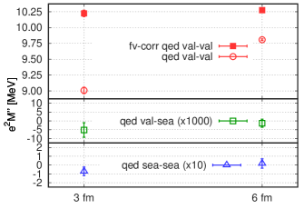
Figure 2: Volume dependence of QED contributions to the $\pi^{+}$ mass at $\beta=3.7000$. The red squares in the upper pane correspond to $M^{\prime\prime}_{20}$ corrected with (17). The valence-sea $M^{\prime\prime}_{11}$ and sea-sea $M^{\prime\prime}_{02}$ contributions are multiplied by 1000 and 10 on the plot, respectively.

3.1 Strong isospin-breaking derivatives$\mathbf{:\langle X\rangle^{\prime}_{m}}$

• $[C^{\text{light}}]^{\prime}_{m}$ is computed via insertion of the operator corresponding to the mass derivative. Since the light propagator is noisy, we evaluate $[C^{\text{conn}}(\kappa m_{l},0)]^{\prime}_{m}$ at multiples $\kappa$ of the light-mass, with $\kappa=3,5,7,9,11$. Then, we perform a chiral extrapolation to $\kappa=1$ to get $[C^{\text{light}}]^{\prime}_{m}$.

• To evaluate the SIB derivative of the disconnected current propagator, we first observe that

  $$[C^{\mathrm{disc}}]^{\prime}_{m}\equiv m_{l}\frac{\partial C^{\mathrm{disc}}}{\partial\delta m}\bigg{|}_{\delta m=e=0}=-\frac{3}{2}m_{l}\frac{\partial C^{\mathrm{disc}}_{0}}{\partial m_{l}}.$$ (18)

  The derivative $\partial C^{\mathrm{disc}}_{0}/\partial m_{l}$ is computed as a finite difference: it is sufficient to evaluate, another light-trace with a slightly different $m_{l}$. We use $I(m_{l},0)$ and $I(0.9~{}m_{l},0)$.

• The SIB derivative of hadron masses is computed as the finite difference

  $$\hskip 20.0ptM^{\prime}_{m}\approx\frac{m_{l}}{\delta m}\left(\mathcal{M}[\langle H_{\delta m}\rangle_{0}]-\mathcal{M}[\langle H_{0}\rangle_{0}]\right)$$ (19)

  where $H_{\delta m}$ is the hadron propagator evaluated at $\delta m=2m_{l}\tfrac{1-r}{1+r}$ with $r=\tfrac{m_{u}}{m_{d}}=0.485$ [8] and $e_{v}=0$.

3.2 Electromagnetic valence-valence derivatives: $\mathbf{\langle X\rangle^{\prime\prime}_{20}}$

• The second derivative $X^{\prime\prime}_{2}$ of an observable $X(e,\delta m)$ can be computed as the finite difference $X^{\prime\prime}_{2}\approx\tfrac{1}{2e_{v}}\left[(X_{+}+X_{-})-2X_{0}\right]$, where $X_{\pm}\equiv X(\pm e_{*},0)$ and $e_{*}$ is the physical value of the electric coupling.

• In the valence-valence case, QED is inserted as a stochastic $U(1)$ field [9]. The statistical noise contributes at order $\mathcal{O}(e)$, but it can be removed by averaging, for each gauge configuration, the two evaluations performed at $\pm e_{v}$ [10].

• To evaluate $[C^{\text{strange}}]^{\prime\prime}_{20}$, we compute $C^{\text{conn}}(m_{s},0)$ and $C^{\text{conn}}(m_{s},\pm\tfrac{1}{3}e_{*})$.

• To evaluate $[C^{\text{light}}]^{\prime\prime}_{20}$, we compute $C^{\text{conn}}(\kappa m_{l},0)$ and $C^{\text{conn}}(\kappa m_{l},\pm\tfrac{1}{3}e_{*})$ for $\kappa=3,5,7,9,11$, then we perform a chiral extrapolation to $\kappa=1$, as for $[C^{\text{light}}]^{\prime}_{m}$.

• The valence-valence derivative of the current disconnected contraction (12) can be computed by rewriting the single contraction, $\sum_{f}q_{f}I_{\mu,x}(m_{f},eq_{f})=\tfrac{2}{3}I(m_{l},\tfrac{2}{3}e)-\tfrac{1}{3}I(m_{l},-\tfrac{1}{3}e)-\tfrac{1}{3}I(m_{s},\tfrac{1}{3}e)$, as $-2I(m_{l},0)+2I(m_{l},\tfrac{1}{3}e)+\tfrac{1}{3}I(m_{l},-\tfrac{1}{3}e)-\tfrac{1}{3}I(m_{s},\tfrac{1}{3}e)$, which equals the first expression when expanding in $e$ up to and including $\mathcal{O}(e^{2})$ terms. The computation of $I(m_{l},0)$, $I(m_{l},\pm\tfrac{1}{3}e_{*})$, $I(m_{s},0)$, and $I(m_{s},\pm\tfrac{1}{3}e_{*})$ is thus sufficient to compute $[C^{\text{disc}}]^{\prime\prime}_{20}$ as a linear combination of finite differences.

• Valence-valence derivatives of hadron masses are computed as the finite difference

  $$M_{20}^{\prime\prime}\approx\frac{1}{2e_{v}^{2}}\left(\mathcal{M}[\langle H_{+}\rangle_{0}]+\mathcal{M}[\langle H_{-}\rangle_{0}]-2\mathcal{M}[\langle H_{0}\rangle_{0}]\right)=\frac{1}{e_{v}^{2}}\left(\mathcal{M}[\tfrac{1}{2}\langle H_{+}+H_{-}\rangle_{0}]-\mathcal{M}[\langle H_{0}\rangle_{0}]\right)$$ (20)

  
  

  and corrected for the finite-volume effects induced by the $\mathrm{QED}_{L}$ scheme, as mentioned above. Here $H_{\pm}$ is the hadron propagator measured at $\delta m=0$ and $e_{v}=\pm e_{*}$.

3.3 Electromagnetic sea-valence derivatives: $\mathbf{\langle X\rangle^{\prime\prime}_{11}}$

• Sea-valence contributions are evaluated as

  $$\langle X\rangle^{\prime\prime}_{11}=\left\langle\left\langle X^{\prime}_{1}\frac{\mathrm{dets}^{\prime}_{1}}{\mathrm{dets}_{0}}\right\rangle_{A}\right\rangle_{U},$$ (21)

  where the subscript $A$ indicates an average over free photon fields, sampled from $e^{-S_{\gamma}}$, and the subscript $U$ an average over dynamical gluon configurations. To estimate the first derivative $\mathrm{dets}^{\prime}_{1}/\mathrm{dets}_{0}$, we generate one photon field $A$ for each gluon field $U$ and $\sim 10^{4}$ random vectors on each $(U,A)$ pair. $X^{\prime}_{1}$ is evaluated as a finite difference: $X^{\prime}_{1}\approx\tfrac{1}{2e_{v}}(X_{+}-X_{-})$.

• Hadron masses are given in the mixed form

  $$M^{\prime\prime}_{11}=\frac{\delta\mathcal{M}}{\delta H}\bigg{|}_{\langle H_{+}+H_{-}\rangle_{0}}\cdot\left\langle\frac{H_{+}-H_{-}}{2e_{v}}\frac{\mathrm{dets}^{\prime}_{1}}{\mathrm{dets}_{0}}\right\rangle,$$ (22)

  with $H_{\pm}$ the hadron propagator evaluated at $\pm e_{*}$ and $\delta m=0$.

3.4 Electromagnetic sea-sea derivatives: $\mathbf{\langle X\rangle^{\prime\prime}_{02}}$

• Sea-sea contributions are evaluated as

  $$\langle X\rangle^{\prime\prime}_{02}=\left\langle[X_{0}-\langle X_{0}\rangle_{U}]\left\langle\frac{\mathrm{dets}^{\prime\prime}_{2}}{\mathrm{dets}_{0}}\right\rangle_{A}\right\rangle_{U}.$$ (23)

  To estimate the second derivative $\mathrm{dets}^{\prime\prime}_{2}/\mathrm{dets}_{0}$, we generate $\sim 2000$ photon fields for each gluon field $U$, and 12 random sources for each photon field $A$.

• Hadron masses are again given in a mixed form:

  $${M^{\prime\prime}_{02}=\frac{\delta\mathcal{M}}{\delta H}\bigg{|}_{\langle H_{0}\rangle_{0}}\cdot\left\langle(H_{0}-\langle H_{0}\rangle)\frac{\mathrm{dets}^{\prime\prime}_{2}}{\mathrm{dets}_{0}}\right\rangle_{0}}.$$

4 Isospin-breaking decomposition

Type-I fits (global fits)

Our simulation has five bare QCD parameters that need to be fixed: $\{a,m_{l},\delta m,m_{s},e\}$, plus the charm mass which is fixed by the strange mass via $m_{c}\equiv 11.85\,m_{s}$.

Given the following definitions for lattice observables (left) and their physical values (right), that can be obtained from the PDG [19],

$$\begin{cases}M_{\pi_{\chi}}^{2}&\equiv\tfrac{1}{2}(M_{uu}^{2}+M_{dd}^{2})\\ M^{2}_{K_{\chi}}&\equiv\tfrac{1}{2}\left(M_{ds}^{2}+M_{us}^{2}-M_{ud}^{2}\right)\\ \Delta M_{K}^{2}&\equiv M_{ds}^{2}-M_{us}^{2}\end{cases}\qquad\begin{cases}[M^{2}_{\pi_{\chi}}]_{*}&\approx[M^{2}_{\pi_{0}}]_{*}\\ [M^{2}_{K_{\chi}}]_{*}&\equiv\tfrac{1}{2}\left([M^{2}_{K_{0}}]_{*}+[M^{2}_{K_{+}}]_{*}-[M^{2}_{\pi_{+}}]_{*}\right)\\ [\Delta M^{2}_{K}]_{*}&\equiv[M^{2}_{K_{0}}]_{*}-[M^{2}_{K_{+}}]_{*}\end{cases}$$ (24)

(with mesons $M_{uu}$ and $M_{dd}$ defined below), a possible way of interpolating to the physical point is to set $a$ using the $\Omega^{-}$ baryon mass $M_{\Omega^{-}}$, the electric charges to $e_{v}\equiv e_{s}\equiv e_{*}=\sqrt{4\pi\alpha_{*}}$ (with $\alpha_{*}$ the experimental value of the fine structure constant, a choice that is valid at leading order in isospin-breaking), and to fix the quark masses by studying the dependence of the observables of interest on $M_{\pi_{\chi}}^{2}$, $M^{2}_{K_{\chi}}$ and $\Delta M_{K}^{2}$ around their physical values:

$$\begin{cases}a=(aM_{\Omega^{-}})/[M_{\Omega^{-}}]_{*}\\ (X_{vv}\equiv e_{v}^{2})=(X_{vs}\equiv e_{v}e_{s})=(X_{ss}\equiv e_{s}^{2})=4\pi\alpha_{*}\\ m_{l}\mid X_{l}\equiv\frac{M_{\pi_{\chi}}^{2}}{M_{\Omega}^{2}}-\frac{[M_{\pi_{\chi}}^{2}]_{*}}{{M_{\Omega}^{2}}_{*}}\quad\text{scatters around}\quad 0\\ m_{s}\mid X_{s}\equiv\frac{M_{K_{\chi}}^{2}}{M_{\Omega}^{2}}-\frac{[M_{K_{\chi}}^{2}]_{*}}{{M_{\Omega}^{2}}_{*}}\quad\text{scatters around}\quad 0\\ \delta m\mid X_{\delta m}\equiv\frac{\Delta M^{2}_{K}}{M_{\Omega}^{2}}\quad\text{scatters around}\quad\frac{[\Delta M^{2}_{K}]_{*}}{[M_{\Omega}^{2}]_{*}}\end{cases}$$ (25)

The specific values of $m_{l},m_{s}$ and $\delta m$ are chosen to be slightly different on each ensemble, such that, altogether, the various measurements bracket the physical point. Thus, one can proceed by parametrizing an observable of interest $O$ with a linear function:

$$O=f(\{X\},A,B,...)\equiv A+BX_{l}+CX_{s}+DX_{\delta m}+EX_{vv}+FX_{vs}+GX_{ss},$$ (26)

where the fit coefficients $A,B,C,F,G$ are polynomials in $a^{2}$, while $D$ and $E$ can also depend on $X_{l}$ and $X_{s}$. For example, $A=A_{0}+A_{2}a^{2}+A_{4}a^{4}$. The continuum extrapolation is then given by

$$O_{*}=A_{0}+D_{0}[X_{\delta m}]_{*}+(E_{0}+F_{0}+G_{0})e_{*}^{2}.$$ (27)

This kind of parametrization, with experimentally measurable quantities as input, is referred as type-I (see Section 3 of [21] or Section 20 of [1] for more details). It is not suitable for an isospin-breaking decomposition (note for example that the observable most sensitive to strong-isospin-breaking effects, $\Delta M_{K}^{2}$, is also charged).

Type-II fits (decomposition-friendly parametrization).

We introduce a second parametrization in order to obtain the decomposition of observables into isospin-symmetric and isospin-breaking parts. We fix the bare parameters $\{a,m_{l},\delta m,m_{s},e\}$ by a new set of observables that we impose to be equal in the isospin-symmetric and full QED+QCD theory:

$$\begin{cases}a=[w_{0}]_{*}/(w_{0}/a)\\ (\tilde{X}_{vv}\equiv e_{v}^{2})=(\tilde{X}_{vs}\equiv e_{v}e_{s})=(\tilde{X}_{ss}\equiv e_{s}^{2})=4\pi\alpha_{*}\\ m_{l}\mid\tilde{X}_{l}\equiv M_{\pi_{\chi}}^{2}w_{0}^{2}-[M_{\pi_{\chi}}^{2}w_{0}^{2}]_{*}\quad\text{scatters around}\quad 0\\ m_{s}\mid\tilde{X}_{s}\equiv M_{ss}^{2}w_{0}^{2}-[M_{ss}^{2}w_{0}^{2}]_{*}\quad\text{scatters around}\quad 0\\ \delta m\mid\tilde{X}_{\delta m}\equiv\Delta M^{2}w_{0}^{2}\quad\text{scatters around}\quad[\Delta M^{2}w_{0}^{2}]_{*}\end{cases}$$ (28)

where

• $w_{0}$ is the Wilson-flow–based, pure-gauge scale defined in [20].

• The masses $M_{uu}$, $M_{dd}$, and $M_{ss}$ are the masses of the neutral mesons $\bar{u}u,\bar{d}d$, and $\bar{s}s$, where only connected diagrams are considered in the propagators. They are neutral and have no magnetic moment (see [22]).

• $\Delta M^{2}=(M_{dd}^{2}-M_{uu}^{2})$ is a measure of strong-isospin-breaking that is not significantly affected by electromagnetic corrections. The equality $\Delta M^{2}=2B_{2}\delta m$ is valid up to effects that are beyond leading order in isospin breaking, as explained in [23].

• $M^{2}_{\pi_{\chi}}=\tfrac{1}{2}(M_{uu}^{2}+M_{dd}^{2})$ equals the neutral pion mass $M^{2}_{\pi^{0}}$ up to terms that are beyond leading order in isospin breaking [23].

Now, the quantities $[w_{0}]_{*}$, $[M^{2}_{ss}]_{*}$ and $[\Delta M^{2}]_{*}$ are not experimentally available. However, they have a well-defined physical continuum limit and can thus be computed using type-I fits. We get the following results:

$$[w_{0}]_{*}=0.17236(29)(63)[70]\,\text{fm}$$

$$[M_{ss}]_{*}=689.89(28)(40)[49]\,\text{MeV}$$

$$[\Delta M^{2}]_{*}=13170(320)(270)[420]\,\text{MeV}^{2}$$

where the errors are statistical, systematic and total respectively.

Isospin decomposition

We write the expectation value of an observable $O$ in QCD+QED, using the set of quantities defined above (the continuum limit is assumed):

$$\langle O\rangle=\langle O\rangle(M_{\pi_{\chi}}w_{0},\,M_{ss}w_{0},\,\tfrac{L}{w_{0}},\,\Delta Mw_{0},\,e),$$ (29)

where $\Delta M=\sqrt{\left(M_{dd}^{2}-M_{uu}^{2}\right)}$. The QED part is defined by switching off the electric charge, keeping the other parameters at their physical values:

$$\langle O\rangle_{\text{QED}}\equiv e^{2}_{*}\cdot\tfrac{\partial\langle O\rangle}{\partial e^{2}}(M_{\pi_{\chi}}w_{0},\,M_{ss}w_{0},\,\tfrac{L}{w_{0}},\,\Delta Mw_{0},\,e=0).$$ (30)

The strong isospin breaking part is defined as the differential

$$\langle O\rangle_{\text{SIB}}\equiv[\Delta Mw_{0}]_{*}^{2}\cdot\tfrac{\partial\langle O\rangle}{\partial(\Delta Mw_{0})^{2}}(M_{\pi_{\chi}}w_{0},\,M_{ss}w_{0},\,\tfrac{L}{w_{0}},\,\Delta Mw_{0}=0,\,e=0).$$ (31)

The isospin-symmetric part is given by the remaining part, computed at $e=\Delta Mw_{0}=0$,

$$\langle O\rangle_{\text{ISO}}\equiv\langle O\rangle(M_{\pi_{\chi}}w_{0},M_{ss}w_{0},\,\tfrac{L}{w_{0}},\,\Delta Mw_{0}=0,\,e=0).$$ (32)

Finally, we show how $\langle O\rangle_{\text{ISO}}$, $\langle O\rangle_{\text{SIB}}$, and $\langle O\rangle_{\text{QED}}$ emerge from the fitting procedure. Our observable $O$ can be parametrized by the linear function

$$O=f(\{\tilde{X}\},\tilde{A},\tilde{B},...)\equiv\tilde{A}+\tilde{B}\tilde{X}_{l}+\tilde{C}\tilde{X}_{s}+\tilde{D}\tilde{X}_{\delta m}+\tilde{E}\tilde{X}_{vv}+\tilde{F}\tilde{X}_{vs}+\tilde{G}\tilde{X}_{ss},$$ (33)

where the fit coefficients $\tilde{A}$, $\tilde{B}$, … have the same form as in (26). If we consider separately each isospin derivative, (33) can be split to a system of five equations:

$$\begin{cases}[O]_{0}=\tilde{A}+\tilde{B}\tilde{X_{l}}+\tilde{C}\tilde{X_{s}}\\ [O]^{\prime}_{m}=[\tilde{D}\tilde{X}_{\delta m}]^{\prime}_{m}\\ [O]^{\prime\prime}_{20}=[\tilde{A}+\tilde{B}\tilde{X}_{l}+\tilde{C}\tilde{X}_{s}+\tilde{D}\tilde{X}_{\delta m}]^{\prime\prime}_{20}+[\tilde{E}]_{0}\\ [O]^{\prime\prime}_{11}=[\tilde{A}+\tilde{B}\tilde{X}_{l}+\tilde{C}\tilde{X}_{s}+\tilde{D}\tilde{X}_{\delta m}]^{\prime\prime}_{11}+[\tilde{F}]_{0}\\ [O]^{\prime\prime}_{02}=[\tilde{A}+\tilde{B}\tilde{X}_{l}+\tilde{C}\tilde{X}_{s}+\tilde{D}\tilde{X}_{\delta m}]^{\prime\prime}_{02}+[\tilde{G}]_{0}\end{cases}$$ (34)

We get the isospin-breaking decomposition after a continuum extrapolation is performed:

$$\langle O\rangle_{\mathrm{ISO}}=\tilde{A}_{0},\qquad\langle O\rangle_{\mathrm{SIB}}=\tilde{D}_{0}\tilde{X}_{\delta m},\qquad\langle O\rangle_{\mathrm{QED}}=e_{*}^{2}(\tilde{E}_{0}+\tilde{F}_{0}+\tilde{G}_{0}),$$ (35)

where $\langle O\rangle_{\mathrm{QED}}=e_{*}^{2}(\tilde{E}_{0}+\tilde{F}_{0}+\tilde{G}_{0})$ can be further separated in

$$\langle O\rangle_{\mathrm{QED-vv}}=e_{*}^{2}\tilde{E}_{0},\qquad\langle O\rangle_{\mathrm{QED-vs}}=e_{*}^{2}\tilde{F}_{0},\qquad\langle O\rangle_{\mathrm{QED-ss}}=e_{*}^{2}\tilde{G}_{0}.$$ (36)

5 Conclusions

QED and strong-isospin-breaking corrections to $a_{\mu}^{\mathrm{LO-HVP}}$ are necessary to reach the precision needed for comparison to experiments. In our work, we have included IB corrections, in current propagators and in hadron masses, by expanding these quantities to first order in the isospin-breaking parameters $\delta m$ and $e^{2}$, and by measuring each term on isospin-symmetric configurations. Furthermore, we have defined an isospin decomposition of observables, which allows us to evaluate the QED and the strong-isospin-breaking contributions to $a_{\mu}^{\mathrm{LO-HVP}}$ summarized in Table 1.

A detailed comparison of isospin-breaking effects computed by different collaborations is a delicate matter, as contributions computed and separation scheme used may differ from group to group. It is nevertheless essential to mention the other works on the subject. Connected valence-valence QED effects have been computed in [26] and [27]. In particular, the strange contribution to this effect is reported in [15] and in the supplemental material of [26]. The connected part of the strong-isospin-breaking effect has been computed in [27, 26, 24] and most recently in [28]. See also [29] for a comparative table and further details.

	$a_{\mu}^{\mathrm{strange}}(L_{\mathrm{ref}},T_{\mathrm{ref}})$	$a_{\mu}^{\mathrm{light}}(L_{\mathrm{ref}},T_{\mathrm{ref}})$	$a_{\mu}^{\mathrm{disc}}(L_{\mathrm{ref}},T_{\mathrm{ref}})$
QED-vv	-0.0086(42)(41)	-1.24(40)(31)	-0.55(15)(10)
QED-vs	-0.0014(11)(14)	-0.0079(86)(94)	0.011(24)(14)
QED-ss	-0.0031(76)(69)	0.37(21)(24)	-0.040(33)(21)
Total QED	-0.0136(86)(76)	-0.93(35)(47)	-0.58(14)(10)
SIB	0	6.60(63)(53)	-4.67(54)(69)
Total IB	-0.0136(86)(76)	5.67(72)(71)	-5.25(56)(70)

Table 1: Continuum extrapolated results for the different components of the strange, light and disconnected, strong and QED isospin-breaking contributions to $a_{\mu}^{\mathrm{LO-HVP}}\times 10^{10}$. Labels v and s refer to valence and sea respectively. The first error is statistical, the second systematic. These results correspond to a box of size $L_{\mathrm{ref}}=6.27~{}\mathrm{fm}$ and $T_{\mathrm{ref}}=\tfrac{3}{2}L_{\mathrm{ref}}$.

References

- [1] S. Borsanyi et al. (BMW Collaboration), Leading hadronic contribution to the muon magnetic moment from lattice QCD, Nature volume 593, pages 51-55 (2021), [hep-lat/2002.12347v3].
- [2] B. Abi et al. (Muon Collaboration), Measurement of the positive muon anomalous magnetic moment to 0.46 ppm, Phys. Rev. Lett. 126, 141801 (2021).
- [3] G. W. Bennett et al. (Muon Collaboration), Final report of the E821 muon anomalous magnetic moment measurement at BNL, Phys. Rev. D 73, 072003 (2006), [hep-ex/0602035].
- [4] T. Aoyama et al. (White paper 2020), The anomalous magnetic moment of the muon in the Standard Model, Phys. Rept. 887, 1-166 (2020) [hep-ph/2006.04822].
- [5] G. M. de Divitiis et al. (RM123 Collaboration), Isospin breaking effects due to the up-down mass difference in Lattice QCD, JHEP 04 124 (2012), [hep-lat/1110.6294].
- [6] G. M. de Divitiis et al. (RM123 Collaboration), Leading isospin breaking effects on the lattice, Phys. Rev. D 87 114505 (2013), [hep-lat/1303.4896].
- [7] M. Hayakawa, & S. Uno, QED in finite volume and finite size scaling effect on electromagnetic properties of hadrons, Prog. Theor. Phys. 120, 413-441 (2008), [hep-lat/0804.2044].
- [8] Z. Fodor, C. Hoelbling, S. Krieg, L. Lellouch, T. Lippert, A. Portelli, A. Sastre, K. K. Szabo and L. Varnhorst, Up and down quark masses and corrections to Dashen’s theorem from lattice QCD and quenched QED, Phys. Rev. Lett. 117, no.8, 082001 (2016) [hep-lat/1604.07112]
- [9] A. Duncan, E. Eichten, & H. Thacker, Electromagnetic splittings and light quark masses inlattice QCD, Phys. Rev. Lett. 76 3894–3897, (1996) [hep-lat/9602005].
- [10] T. Blum, T. Doi, M. Hayakawa, T. Izubuchi, & N. Yamada, Determination of light quark masses from the electromagnetic splitting of pseudoscalar meson masses computed with two flavors of domain wall fermions, Phys. Rev. D 76 114508, (2007) [hep-lat/0708.0484].
- [11] G. S. Bali, S. Collins, & A. Schafer, Effective noise reduction techniques for disconnected loops in Lattice QCD, Comput. Phys. Commun. 181, 1570–1583 (2010), [hep-lat/0910.3970]
- [12] T. Blum, T. Izubuchi, & E. Shintani, New class of variance-reduction techniques using lattice symmetries, Phys. Rev. D 88, 094503 (2013), [hep-lat/1208.4349]
- [13] H. Neff, N. Eicker, T. Lippert, J. W. Negele, & K. Schilling, On the low fermionic eigenmode dominance in QCD on the lattice, Phys. Rev. D 64, 114509 (2001), [hep-lat/0106016].
- [14] A. Li et al. (QCD Collaboration), Overlap Valence on 2+1 Flavor Domain Wall Fermion Configurations with Deflation and Low-mode Substitution, Phys. Rev. D 82, 114501 (2010), [hep-lat/1005.5424].
- [15] D. Giusti, V. Lubicz, G. Martinelli, F. Sanfilippo, and S. Simula (ETM Collaboration), Strange and charm HVP contributions to the muon (g-2) including QED corrections with twisted-mass fermions, JHEP 10, 157 (2017), [hep-lat/1707.03019].
- [16] Borsanyi, S. et al., Hadronic vacuum polarization contribution to the anomalous magnetic moments of leptons from first principles, Phys. Rev. Lett. 121, 022002 (2018), [hep-lat/1711.04980]
- [17] Z. Davoudi, & M. J. Savage, Finite-Volume Electromagnetic Corrections to the Masses of Mesons Baryons and Nuclei, Phys. Rev. D 90, 054503 (2014), [hep-lat/1402.6741].
- [18] Borsanyi, S. et al., Ab initio calculation of the neutron-proton mass difference, Science 347, 1452–1455 (2015), [hep-lat/1406.4088v2].
- [19] P.A. Zyla et al. [Particle Data Group], Review of Particle Physics, PTEP 2020, no.8, 083C01 (2020).
- [20] S. Borsanyi, et al., High-precision scale setting in lattice QCD, JHEP 09, 010. (2012), [hep-lat/1203.4469].
- [21] L. Varnhorst et al., High precision scale setting on the lattice, PoS LATTICE2021 371 (2022).
- [22] S. Borsanyi, et al., Isospin splittings in the light baryon octet from lattice QCD and QED, Phys. Rev. Lett. 111, 252001 (2013), [hep-lat/1306.2287].
- [23] J. Bijnens, & N. Danielsson, Electromagnetic Corrections in Partially Quenched Chiral Perturbation Theory, Phys. Rev. D 75, 014505 (2007), [hep-lat/0610127].
- [24] B. Chakraborty et al. (Fermilab Lattice, HPQCD, and MILC Collaborations), Strong-Isospin-Breaking Correction to the Muon Anomalous Magnetic Moment from Lattice QCD at the Physical Point, Phys. Rev. Lett. 120, 152001 (2018), [hep-lat/1710.11212].
- [25] C. T. H. Davies et al., Hadronic-vacuum-polarization contribution to the muon’s anomalous magnetic moment from four-flavor lattice QCD, Phys. Rev. D 101, 034512 (2020), [hep-lat/1902.04223].
- [26] T. Blum et al. (RBC and UKQCD Collaborations), Calculation of the Hadronic Vacuum Polarization Contribution to the Muon Anomalous Magnetic Moment, Phys. Rev. Lett. 121, 022003 (2018), (and Supplemental Material).
- [27] D. Giusti, V. Lubicz, G. Martinelli, F. Sanfilippo, & S. Simula, Electromagnetic and strong isospin-breaking corrections to the muon g-2 from Lattice QCD+QED., Phys. Rev. D 99, 114502 (2019), [hep-lat/1901.10462].
- [28] C. Lehner and A. S. Meyer, Consistency of hadronic vacuum polarization between lattice QCD and the R ratio, Phys. Rev. D 101, 074515 (2020), [hep-lat/2003.04177].
- [29] A. Gérardin, The anomalous magnetic moment of the muon: status of Lattice QCD calculations, Eur. Phys. J. A. 57 4, 116 (2021), [hep-lat/2012.03931].