“Stairway to Heaven” – Spectroscopy of Particle Couplings with Gravitational Waves

Abstract

We discuss the possibility to measure particle couplings with stochastic gravitational wave backgrounds (SGWBs). Under certain circumstances a sequence of peaks of different amplitude and frequency – a stairway –, emerges in a SGWB spectrum, with each peak probing a different coupling. The detection of such signature opens the possibility to reconstruct couplings (spectroscopy) of particle species involved in high energy phenomena generating SGWBs. Stairway-like signatures may arise in causally produced backgrounds in the early Universe, e.g. from preheating or first order phase transitions. As a proof of principle we study a preheating scenario with an inflaton $\phi$ coupled to multiple daughter fields $\{\chi_{j}\}$ with different coupling strengths. As a clear stairway signature is imprinted in the SGWB spectrum, we reconstruct the relevant couplings with various detectors.

Introduction. Gravitational wave (GW) astronomy has emerged as an exciting new field initiated by the detection of GWs by the LIGO/Virgo network, yielding outstanding results on the relativistic dynamics of compact binaries, and enabling stringent tests of gravity, see e.g. Abbott et al. (2016a, b, 2019a); Venumadhav et al. (2020); Abbott et al. (2021, 2017a, 2017b). This new observational probe offers as well unprecedented opportunities for breakthroughs in high-energy physics and early universe cosmology. The key point to note is that early universe dynamics operate at energies unreachable by any terrestrial means, sourcing stochastic GW backgrounds (SGWBs) that carry information about the phenomena that created them. Cosmological SGWBs of diverse origin are in fact expected to permeate the Universe, see Caprini and Figueroa (2018); Maggiore (2018) for reviews.

As supported by cosmic microwave background (CMB) observations Akrami et al. (2020), we assume an early phase of accelerated expansion, inflation, as the framework to explain the initial conditions of the universe Guth (1981); Linde (1982); Albrecht and Steinhardt (1982); Brout et al. (1978); Starobinsky (1980); Kazanas (1980); Sato (1981); Mukhanov and Chibisov (1981); Guth and Pi (1982); Starobinsky (1982); Hawking (1982). SGWBs arise naturally due to quantum vacuum fluctuations in vanilla inflation models Grishchuk (1974); Starobinsky (1979); Rubakov et al. (1982); Fabbri and Pollock (1983), as well as from complicated dynamics of axion-like species present during inflation, see e.g. Anber and Sorbo (2006); Sorbo (2011); Pajer and Peloso (2013); Adshead et al. (2013a, b); Maleknejad (2016); Dimastrogiovanni et al. (2017); Namba et al. (2016); Ferreira et al. (2016); Peloso et al. (2016); Domcke et al. (2016); Caldwell and Devulder (2018); Guzzetti et al. (2016); Bartolo et al. (2016); D’Amico et al. (2021a, b). Inflation is followed by a (p)reheating stage, converting the energy available into particle species that eventually dominate the energy budget Allahverdi et al. (2010); Amin et al. (2014); Lozanov (2019); Allahverdi et al. (2020). SGWBs are expected from particle production during preheating Easther and Lim (2006); Garcia-Bellido and Figueroa (2007); Garcia-Bellido et al. (2008a); Dufaux et al. (2007, 2009, 2010); Bethke et al. (2013, 2014); Figueroa and Torrenti (2017a); Adshead et al. (2018, 2020a, 2020b), and from various post-inflationary phenomena, like kination-domination Giovannini (1998, 1999); Boyle and Buonanno (2008); Figueroa and Tanin (2019a, b); Gouttenoire et al. (2021), oscillon dynamics Zhou et al. (2013); Antusch et al. (2017, 2018); Liu et al. (2018); Amin et al. (2018), strong first order phase transitions Kamionkowski et al. (1994); Caprini et al. (2008); Huber and Konstandin (2008); Hindmarsh et al. (2014, 2015); Caprini et al. (2016); Hindmarsh et al. (2017); Cutting et al. (2018, 2018, 2020); Roper Pol et al. (2020); Cutting et al. (2021), or cosmic defects Vachaspati and Vilenkin (1985); Sakellariadou (1990); Damour and Vilenkin (2000, 2001, 2005); Figueroa et al. (2013); Hiramatsu et al. (2014); Blanco-Pillado and Olum (2017); Auclair et al. (2020); Figueroa et al. (2020); Caprini et al. (2020); Gorghetto et al. (2021); Chang and Cui (2021).

A detection program including a large variety of experiments, and covering a wide range of frequencies, is slowly emerging. These experiments range from increasingly precise CMB and pulsar timing array observations Abazajian et al. (2016); Arzoumanian et al. (2020), to present and proposed GW direct detection experiments Sesana et al. (2021); Amaro-Seoane et al. (2017); Ruan et al. (2020); Baker et al. (2019); Kawamura et al. (2011); Somiya (2012); Mei et al. (2020); Kuns et al. (2020); Reitze et al. (2019); Punturo et al. (2010); Abbott et al. (2019b) and atom interferometers Graham et al. (2017); El-Neaj et al. (2020), altogether spanning $\sim 20$ decades in frequency, from $\sim 10^{-17}$ Hz to $\sim$ kHz. Furthermore, a high-frequency detection program at $\sim$ MHz frequencies and above, has just been recently put forward Aggarwal et al. (2020). An evaluation of the ability of many of these experiments to probe new high energy physics is still in progress.

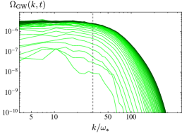
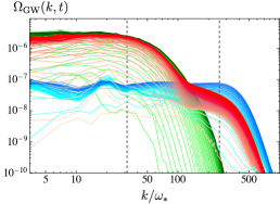
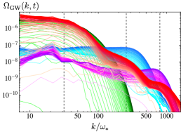
Figure 1: Left: GW spectrum from a single daughter field with $q=3\times 10^{4}$. Middle: GW spectra from single daughter field with $q_{1}=3\times 10^{4}$ (green) and $q_{2}=1.5\times 10^{6}$ (blue). A two-peak spectrum (red) emerges when the two daughter fields are simultaneously coupled to the inflaton, with the same couplings as in the single daughter cases. Right: GWs from three single daughter fields for $q_{1}=3\times 10^{4}$ (green), $q_{2}=1.5\times 10^{6}$ (blue) and $q_{3}=1.3\times 10^{7}$ (purple). A three-peak spectrum appears when the three daughter fields are simultaneously coupled to the inflaton, with the same couplings as the single daughter cases. In all plots vertical dashed lines show the prediction of Eq. (4) for the peak position from single daughter simulations.

In this letter we propose to measure particle couplings with GWs. While in particle colliders one looks for features in statistical observables, we look instead for features in SGWB spectra. Considering early Universe scenarios sourcing GWs, we address the question of how the presence of multiple fields, all contributing to GW production, affect the SGWB spectrum. This question does not have a unique or immediate answer. Indeed, while the source of GWs is a linear superposition of individual contributions, the SGWB spectrum is quadratic in the source. Furthermore, the dynamics of the different fields in the multi-field system may differ from their single-field dynamics. Under certain circumstances, however, a sequence of peaks of different amplitude and frequency – a stairway –, may emerge in the SGWB spectrum, probing the leading interaction of each individual species. Detecting such signature would allow to reconstruct the relevant couplings (spectroscopy) of the field species involved in high energy phenomena generating SGWBs.

As a proof of principle, we consider a preheating scenario where an inflaton $\phi$ oscillates around the minimum of its potential, while multiple daughter fields $\{\varphi_{j}\}$ are coupled to the inflaton, each with different coupling strength. When the couplings are large enough, the daughter species are excited in broad parametric resonance, developing spectra that are peaked at scales determined by their coupling strength. By studying the SGWB sourced by various daughter fields, we show that, in fact, a stairway of peaks of different amplitude and frequency, emerges in the SGWB spectrum. As each peak probes a different coupling, the detection of such signature allows for a reconstruction of the coupling constants. Our working scenario represents a compelling case of the ability of SGWBs to probe particle couplings.
Stairway in the SGWB. We assume summation over repeated indices and consider a spatially flat Friedmann–Lemaître–Robertson–Walker (FLRW) background with tensor perturbations, $ds^{2}=-dt^{2}+a^{2}(t)(\delta_{ij}+h_{ij})dx^{i}dx^{j}$, with $a(t)$ the scale factor, and the perturbations verifying $h_{ii}=\partial_{i}h_{ij}=0$. We denote as $m_{p}=1/\sqrt{8\pi G}=2.44\cdot 10^{18}$ GeV the reduced Planck mass.

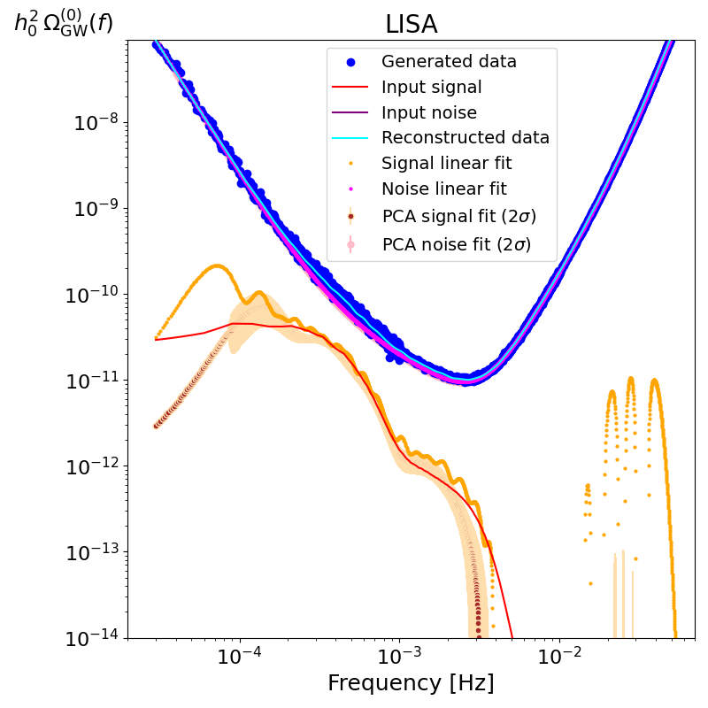
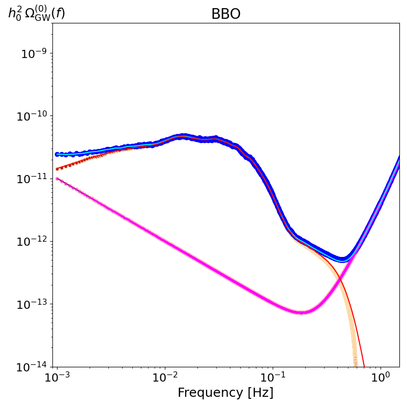
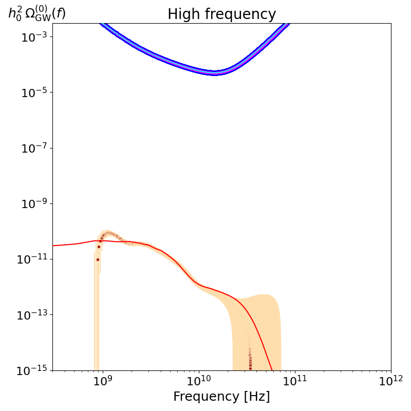
Figure 2: Signal and noise reconstructions using Principal Component Analysis over a two-peak GW signal with $q_{1}=3\cdot 10^{4}$ and $q_{2}=1.5\cdot 10^{6}$, for LISA (left panel), BBO (central panel) and a speculative High Frequency Experiment (HFE, right panel).

We consider an observationally viable inflationary model inspired by $\alpha$-attractors Kallosh and Linde (2013), with the inflaton $\phi$ coupled to a set of daughter scalar fields $\{\chi_{j}\}$,

$$V(\phi,\{\chi_{j}\})=\dfrac{1}{2}\Lambda^{4}\tanh^{2}{\left(\dfrac{\phi}{M}\right)}+\dfrac{1}{2}g_{j}^{2}\chi_{j}^{2}\phi^{2}\,.$$ (1)

We fix $M=5\,m_{p}$ and $\Lambda=0.00564\,m_{p}$ for compatibility with CMB constraints, and keep free the coupling constants $g_{j}^{2}$. The inflaton potential flattens out for $|\phi|\gg M$, and takes the form $V\simeq{1\over 2}\omega_{*}^{2}\phi^{2}$ for $|\phi|\ll M$, with $\omega_{*}=\Lambda^{2}/M$. We choose quadratic interactions as these are scale-free and serve as a proxy for the leading term in scalar-gauge interactions Figueroa et al. (2015). Preheating takes place via broad parametric resonance, as the oscillations of the homogeneous inflaton induce an exponential growth of the preheat mode functions ${\chi}_{j}(k,t)$. The resonance of each species is controlled by their resonance parameter $q_{j}=g_{j}^{2}\phi_{*}^{2}/\omega_{*}^{2}\gg 1$, with $\phi_{*}\simeq 0.95\,m_{p}$ the inflaton amplitude at the end of inflation. Modes of each preheat species are exponentially excited during the initial linear regime, up to a co-moving scale $k\lesssim k_{l}^{(j)}\sim\omega_{*}q_{j}^{1/4}$ Kofman et al. (1997). Eventually, the preheat fields back-react into the inflaton, and the dynamics become non-linear. As a result, mode-to-mode interactions populate higher momenta beyond the linear threshold, typically up to a peak scale $k_{p}^{(j)}\sim\omega_{*}q_{j}^{p}$, $p\gtrsim 0.5$ Figueroa and Torrenti (2017a). Modes with $k>k_{p}^{(j)}$ are exponentially suppressed. The system reaches eventually a stationary state characterised by no significant transfer of energy among species Figueroa and Torrenti (2017b); Antusch et al. (2020, 2021).

The dynamics of the fields lead to an anisotropic stress with non-vanishing transverse-traceless (TT) part $\Pi_{ij}^{\rm TT}=\{\partial_{i}\phi\partial_{j}\phi\ +\partial_{i}\chi_{a}\partial_{j}\chi_{a}\}^{\rm TT}$. GWs are then sourced by all field species, with the GW dynamics governed by $(\partial^{2}_{t}+3H\partial_{t}-a^{-2}\nabla^{2})h_{ij}=2m_{p}^{-2}a^{-2}\Pi_{ij}^{\rm TT}$, with $H=\dot{a}/a$ the Hubble rate. The SGWB energy density spectrum, normalized to the critical energy density $\rho_{c}$, is given by

$$\Omega_{\rm GW}(k,t)\equiv\dfrac{1}{\rho_{c}}\frac{d\rho_{\rm GW}}{d\log k}\,,~{}~{}~{}\frac{d\rho_{\rm GW}}{d\log k}=\frac{k^{3}\mathcal{P}_{\dot{h}}(k,t)}{(4\pi)^{3}G}\,,$$ (2)

$$\langle\dot{{h}}_{ij}\left(\mathbf{k},t\right)\dot{{h}}_{ij}^{*}\left(\mathbf{k^{\prime}},t\right)\rangle\equiv(2\pi)^{3}\,\mathcal{P}_{\dot{h}}(k,t)\,\delta({\bf k}-{\bf k}^{\prime})\,,$$ (3)

with $\langle...\rangle$ representing stochastic averaging Lat . In this scenario GWs are actively sourced untill the start of the stationary regime, and propagate freely afterwards.

The non-linear dynamics of the system can only be studied with lattice simulations. We have added for this purpose GW dynamics into the package ${\mathcal{C}}$osmo${\mathcal{L}}$attice Figueroa et al. (2021a); mod . By running simulations with a single daughter field for different coupling constants $g^{2}$, we have parametrized the peak’s position ($k_{p}$) and amplitude ($\Omega_{\rm GW}^{(p)}\equiv\Omega_{\rm GW}(k_{p})$) of single-daughter SGWB spectra as a function of $q={g^{2}\phi_{*}^{2}/\omega_{*}^{2}}$. By measuring spectra at a time $\omega_{*}t_{\rm f}=600$, we guarantee (for all couplings used) that the system is in the stationary regime when GW production ceases. We obtain (for $q\gtrsim 10^{4}$)

$$k_{p}(q)/\omega_{*}=(21.22\pm 7.64)\left(\dfrac{q}{10^{4}}\right)^{0.52\pm 0.08}~{}~{}~{}~{}~{}\,,$$ (4)

$$\Omega_{\rm GW}^{(p)}(q)=(1.2\pm 0.7)\times 10^{-5}\left(\dfrac{q}{10^{4}}\right)^{-1.1\pm 0.12}\,,$$ (5)

It is clear from Eqs. (4), (5) that sufficiently separated values of $q$ lead to single-daughter spectra with quite different amplitudes and peak frequencies. In realistic scenarios we naturally expect various daughter fields to be present. If these are coupled to the inflaton with different coupling strengths, relevant questions can then be raised: will the final SGWB spectrum be the superposition of each individual daughter’s spectrum? do interference effects affect the final spectral shape? can we expect a series of peaks to emerge at the positions indicated by single daughter field spectra?

In Fig. 1 we plot SGWB spectra from single daughter simulations (left, central and right panels), and superimpose the spectrum from simulations with two (central panel) or three (right panel) daughter fields, with the same couplings as the single daughter cases. The plots are self-explanatory: a stairway signature consisting of a series of peaks, as many as the daughter fields, emerges clearly in the multi-daughter spectra. As the energy must be split between the different species, the stairway peak amplitudes are smaller than in the individual daughter field spectra. The position of the stairway peaks, however, is still well predicted by the single-daughter spectra prediction Eq. (4). Redshifting the background, the peak frequencies of a signal today is approximated as Fre

$$f_{\rm p}\simeq 4\cdot 10^{10}\times\left({H_{\rm f}\over m_{p}}\right)^{1/2}\times{k_{p}(q)\over a_{\rm f}H_{\rm f}}\,\,~{}{\rm Hz}\,.$$ (6)

where $H_{\rm f}=H(t_{\rm f})$ and $a_{\rm f}=a(t_{\rm f})$. To separate clearly the peaks we need $q_{j}/q_{i}\gtrsim{\rm few}\times 10$. It is also important that interactions among daughter species are negligible during GW production (in our calculations we simply neglected daughter-to-daughter interactions).

Particle coupling spectroscopic reconstruction. Using data analysis techniques Caprini et al. (2019); Pieroni and Barausse (2020); Flauger et al. (2021) we reconstruct next multi-peak SGWB spectra generated with our simulations, and turn the reconstruction into constrains on the particle couplings thanks to Eqs. (4), (6).

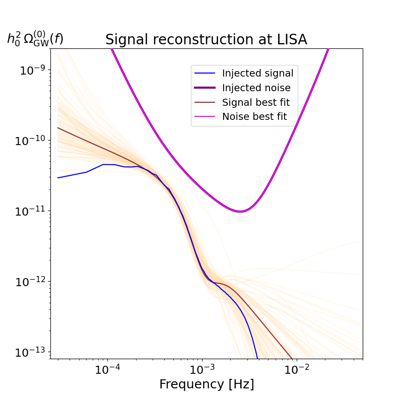
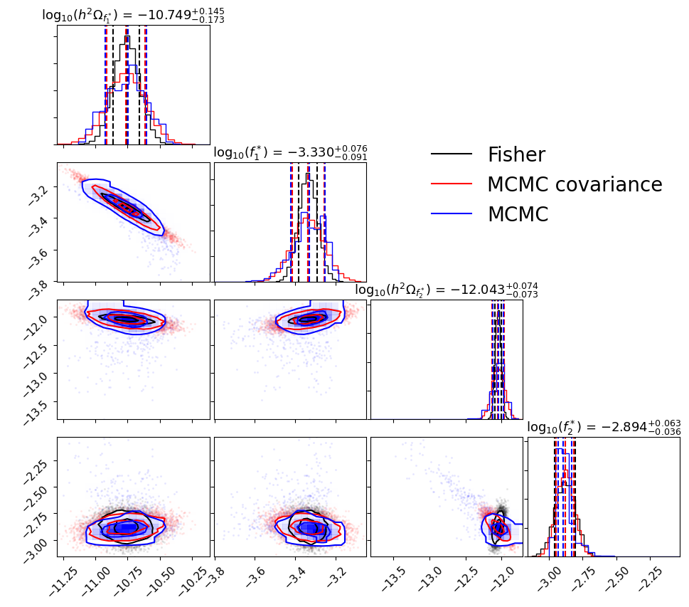
Figure 3: Left: Signal and noise reconstruction of a double peaked signal at LISA (see main text for details). The $2\sigma$ signal and noise error bands are shown in orange and pink respectively. Right: Corner plot for some of the signal parameters showing the $1$ and $2\sigma$ regions. The blue curves are the MCMC chains results, the red curves correspond to the covariance matrix obtained from the MCMC chains and in black we show the constrains obtained with a Fisher matrix approach.

After generating data sets from our GW signals (see supplementary material), we first apply the Principal Component Analysis (PCA) method of Pieroni and Barausse (2020). This is a model independent procedure for reconstructing an unknown signal by first expanding it onto a general basis of functions, and then dropping the low information components of the Fisher Information Matrix (FIM), $F_{\alpha\beta}\equiv\langle-\frac{\partial^{2}\ln\mathcal{L}}{\partial\theta^{\alpha}\partial\theta^{\beta}}\rangle$.

Plugging Eq. (4) into Eq. (6), leads to SGWB peak frequencies around $\sim 100$ MHz for $q_{j}\sim 10^{4}-10^{6}$. These frequencies are way above the range accessible to present GW direct detection experiments like LIGO Aasi et al. (2015), Virgo Acernese et al. (2015) and KAGRA Kawamura et al. (2011), planned detectors like LISA Amaro-Seoane et al. (2017), ET Punturo et al. (2010), or even futuristic projects like BBO Harry et al. (2006). While other multi-field scenarios might produce SGWBs with stairway signatures at observable frequencies, like hybrid preheating scenarios Dufaux et al. (2010); Tranberg et al. (2018); Cui and Sfakianakis (2021) or first order phase transitions Kamionkowski et al. (1994); Caprini et al. (2008); Huber and Konstandin (2008); Hindmarsh et al. (2014, 2015); Caprini et al. (2016); Hindmarsh et al. (2017); Cutting et al. (2018, 2018, 2020); Roper Pol et al. (2020); Cutting et al. (2021) with gauge fields, any characterization of their potential spectroscopic signatures requires dedicated studies currently unavailable. In order to proceed with a coupling reconstruction, we consider instead, for simplicity, that our multi-peak SGWB spectra serve as a template for lower-frequency signal scenarios. We thus shift by hand today’s SGWB spectra by a fudge factor $\alpha_{\rm exp}\equiv f_{\rm exp}/f_{p}$, while leaving their amplitudes intact. The shifted backgrounds peak therefore at some typical frequency $f_{\rm exp}$ of a given experiment. By choosing $\alpha_{\rm LISA}=1.11\cdot 10^{-13}$ and $\alpha_{\rm BBO}=1.55\cdot 10^{-11}$, we analyze the capability of LISA and BBO to reconstruct SGWB spectra with stairway structures given by our simulation-generated templates. Furthermore, we also introduce a speculative futuristic high-frequency experiment (HFE) capable of detecting our SGWBs at their natural high-frequencies.

Examples of a 2-peak signal reconstruction are shown in Fig 2, performed respectively with: i) LISA, using the noise model from Flauger et al. (2021); Babak et al. (2021), ii) BBO, using the noise model from Crowder and Cornish (2005); Harry et al. (2006), and iii) a futuristic high frequency experiment (HFE), the sensitivity of which we construct ad hoc in such a way that the signal has roughly the same signal-to-noise ratio as in LISA when shifting the LISA noise curve, see Fig 2. The two peaks in the signal are clearly identified in the three cases. By using our procedure, together with alternative methods Caprini et al. (2019); Flauger et al. (2021), it is possible to reconstruct the SGWB frequency shape in an agnostic way. Once an appropriate shape has been identified, a direct search can be actually used in order to directly constrain the model parameters. For this purpose we use the same likelihood as in Eq.(3.12) of Flauger et al. (2021), and model a general $n$-peaked signal as a sum of power law signals with exponential cut-offs:

$$h^{2}\Omega_{GW}=\sum_{i=1}^{n}10^{\ln\left(h^{2}\Omega^{*}_{i}\right)}\frac{2\left(\frac{f}{f^{*}_{i}}\right)^{n_{i}}}{1+\exp\left\{\frac{\delta_{i}(f-f^{*}_{i})}{f^{*}_{i}}\right\}}\;,$$ (7)

where $h_{0}\equiv H_{0}$[Mpc/Km/s]$/100$ characterises today’s Hubble rate, $h_{0}^{2}\Omega^{*}_{i}$ denotes the amplitude of the $n$-th signal in the peak frequency $f^{*}_{i}$, $n_{i}$ its power-law tilt, and $\delta_{i}>0$ controls the strength of the exponential suppression. In Fig. 3 we show the results obtained by injecting the same signal used in the left panel of Fig 2, and simultaneously fitting for signal and noise with LISA. The parameter space is sampled using Polychord Handley et al. (2015a, b) via its interface with Cobaya Torrado and Lewis (2021). In the left panel we show the reconstruction of the signal and of the noise as compared to the injections, and in the right panel we show the contour plots for the amplitudes and pivot frequencies of the two-peak spectra (after marginalizing over all other parameters). For reference we compare with results obtained with a Fisher matrix approach which only includes the signal parameters. As seen in the figure, the deviation between the two results is minimal, what implies that the inclusion of noise parameters does not significantly affect the reconstruction of the signal.

In the three cases we reconstruct the coupling constants as indicated in Table 1, for a GW signal obtained from a two-daughter field simulation with $q_{1}=3\cdot 10^{4}$ and $q_{2}=1.5\cdot 10^{6}$. The determination of the peak frequencies and their errors for each experiment (for BBO and HFE we use a FIM approach), leads to a reconstruction of the resonance parameters inverting Eqs. (4) & (6), from where we obtain the coupling constants. While the numerical reconstruction of $q_{i}$’s and $g_{i}$’s is only precise to within the order of magnitude, it is remarkable that all reconstructed values are compatible at $1\sigma$ with the injected values. This clearly indicates the great potential for particle coupling spectroscopy that SGWB detection may offer in the future.

	LISA	BBO	HFE
$\log_{10}(f_{1}^{*}{\rm[Hz]})$	$-3.33^{+0.08}_{-0.09}$	$-1.539^{+0.002}_{-0.002}$	$9.45^{+0.15}_{-0.15}$
$q_{1}=3\cdot 10^{4}$	$6.14^{+29.86}_{-4.10}\cdot 10^{4}$	$1.28^{+2.45}_{-0.62}\cdot 10^{4}$	$2.83^{+17.88}_{-2.06}\cdot 10^{4}$
$g_{1}=1.16\cdot 10^{-3}$	$1.66^{+4.01}_{-0.55}\cdot 10^{-3}$	$0.76^{+0.73}_{-0.18}\cdot 10^{-3}$	$1.13^{+3.56}_{-0.41}\cdot 10^{-3}$
$\log_{10}(f_{2}^{*}{\rm[Hz]})$	$-2.89^{+0.06}_{-0.04}$	$-0.496^{+0.001}_{-0.001}$	$10.4^{+0.4}_{-0.4}$
$q_{2}=1.5\cdot 10^{6}$	$0.43^{+2.8}_{-0.3}\cdot 10^{6}$	$1.3^{+7.42}_{-0.89}\cdot 10^{6}$	$1.9^{+108.65}_{-1.78}\cdot 10^{6}$
$g_{2}=8.2\cdot 10^{-3}$	$4.39^{+14.3}_{-1.53}\cdot 10^{-3}$	$7.64^{+21.8}_{-2.61}\cdot 10^{-3}$	$9.23^{+263.9}_{-4.32}\cdot 10^{-3}$

Table 1: Numerical reconstruction of frequency peaks, resonance parameters and coupling constants.

Discussion.– Realistic early universe scenarios are naturally expected to contain multiple fields, as there is no symmetry or fundamental principle that implies otherwise. The Standard Model (SM), between matter and gauge fields, contains dozen of fields. Beyond the SM (BSM) scenarios only add up to this argument. In this Letter, we discuss the possibility to measure particle couplings through SGWBs. We focus on the emergence of a sequence of peaks of different amplitude and frequency, a stairway, in the SGWB spectrum produced in scenarios with multiple particle species involved in the GW generation. As a proof of principle we have studied a preheating scenario with an oscillating inflaton $\phi$, coupled simultaneously to multiple daughter fields $\{\varphi_{j}\}$, interacting though $g_{j}^{2}\varphi_{j}^{2}\phi^{2}$ with different coupling strengths. When the daughter species are excited, we show that a stairway signature with as many peaks as fields $\{\varphi_{j}\}$, is imprinted in the SGWB spectrum, with each peak probing the interaction strength of each individual species.

Our working scenario represents a compelling case of the ability of SGWBs to probe particle couplings. We have assumed a quadratic potential $V\propto\phi^{2}$ during the inflation oscillations, so that only daughter field peaks are imprinted. If a different shape was considered, say e.g. $V\propto\phi^{p}$ with $p\neq 2$ or a linear combination of monomials, inflaton self-resonance will possibly create new peaks in the SGWB spectrum. For simplicity we have assumed the same type of quadratic interactions $\propto\varphi_{j}^{2}\phi^{2}$ for all daughter species. We expect however the emergence of analogous stairway signatures in the SGWB spectrum when other interactions are considered, like those in tachyonic preheating Felder et al. (2001a, b); Garcia-Bellido et al. (2003); Copeland et al. (2002); Dufaux et al. (2010); Tranberg et al. (2018), axion preheating Adshead et al. (2015); Cuissa and Figueroa (2019); Adshead et al. (2020a); Cui and Sfakianakis (2021), or geometric preheating Bassett and Liberati (1998); Tsujikawa et al. (1999); Fu et al. (2019); Figueroa et al. (2021b). In the case of strong first order phase transitions (see e.g. Hindmarsh et al. (2021) for a review), gauge fields coupled to the corresponding Higgs sector of the theory will be inevitably excited during the nucleation and collision of bubbles. Arguably this should lead to new peaks in the SGWB spectrum probing the Higgs-gauge couplings.

We note that in our numerical calculations we have assumed that interactions among the daughter species are negligible within the time scale of GW generation. If daughter-to-daughter interactions were active during GW production, this would affect their dynamics, for example re-distributing power differently among them. The presence of such interactions may therefore affect significantly the peak structure of the resulting stairway in the SGWB spectrum, an aspect we hope we to return to in a future investigation.

Acknowledgements–. We thank Robert Plant, Jimmy Page, John Paul Jones and John Bonham for suggesting a nice title for our paper and for providing great inspiration and good times. DGF is supported by a Ramón y Cajal contract with Ref. RYC-2017-23493. AF is supported by the U.S. Department of Energy, Office of Science, Office of Nuclear Physics, grants Nos. DE-FG88ER40388. NL is supported by project PROMETEO/2019/083 from Generalitat Valenciana. The work of M.P. was supported by STFC grants ST/P000762/1 and ST/T000791/1. M.P. acknowledges support by the European Union’s Horizon 2020 Research Council grant 724659 MassiveCosmo ERC- 2016-COG. This work is also supported by PROMETEO/2021/083 from Generalitat Valenciana, and by PID2020-113644GB-I00 from Ministerio de Ciencia e Innovación. We are also very thankful for the use of computational resources provided by Finis-Terrae II cluster of CESGA (Centro de Supercomputación de Galicia), Vives and Tirant clusters of Universitat de Valencia.

I Supplemental material

Background redshift. The SGWB today is obtained by redshifting the amplitude and frequency of the background from the end of GWs production $t_{end}$, following the appropriate expansion history of the Universe. Given that we know the expansion history up to the final time $t_{\rm f}$ of our simulations, and noticing that $t_{end}<t_{\rm f}$, we can apply the redshifting from $t_{\rm f}$ until the present time $t_{0}$. Let us characterize the expansion history between $t_{\rm f}$ and the onset of radiation domination (RD) at $t_{\rm RD}$, with an effective equation of state $\bar{w}=p/\rho$

$$\begin{array}[]{cc}\log\left(\dfrac{\rho^{\rm(RD)}_{tot}}{\rho^{\rm(f)}_{tot}}\right)&=-3\int^{a_{\rm RD}}_{a_{\rm f}}\dfrac{da^{\prime}}{a^{\prime}}(1+w(a^{\prime}))\>,\\ &=-3(1+\bar{w})\log\left(\dfrac{a_{\rm RD}}{a_{\rm f}}\right)\>,\end{array}$$ (8)

The SGWB spectrum actually peaks at some sub-horizon scale $k_{p}=\beta_{p}a_{\rm f}H_{\rm f}$, with $a_{\rm f}=a(t_{\rm f})$ and $H_{\rm f}=H(t_{\rm f})$. We expect the SGWB spectrum to peak therefore at a frequency $f_{\rm GW}$ today

$$f_{\rm GW} \equiv \dfrac{k_{\rm GW}}{2\pi a_{0}}=\dfrac{\beta_{\rm GW}}{2\pi}\left(\dfrac{a_{\rm f}}{a_{\rm RD}}\right)\left(\dfrac{a_{\rm RD}}{a_{0}}\right)H_{\rm f}$$ (9)

$$= \dfrac{\beta_{\rm GW}}{2\pi}\left(\dfrac{a_{\rm f}}{a_{\rm RD}}\right)G_{\rm RD}^{1/4}\left(\dfrac{\rho_{rad,0}}{\rho_{\rm rad,RD}}\right)^{1/4}H_{\rm f}$$

$$= \dfrac{\beta_{\rm GW}}{2\pi}(2\epsilon_{\rm f})^{1/4}G_{\rm RD}^{1/4}\left(\dfrac{H_{\rm f}}{\rho_{\rm rad,RD}}\right)^{1/4}\rho_{\rm rad,0}$$

$$= \dfrac{k_{p}}{a_{\rm f}H_{\rm f}}\epsilon_{\rm f}^{1/4}G_{\rm RD}^{1/4}\left(\dfrac{H_{\rm f}}{m_{p}}\right)^{1/2}\left(\dfrac{2}{3}\right)^{1/4}\dfrac{\rho_{\rm rad,0}^{1/4}}{2\pi}\,,$$

where we have defined

$$\epsilon_{\rm f}\equiv\left(\dfrac{a_{RD}}{a_{\rm f}}\right)^{1-3\bar{w}}\,,~{}~{}G_{RD}\equiv\left(\dfrac{g_{RD}}{g_{0}}\right)\left(\dfrac{g_{s,0}}{g_{s,RD}}\right)^{4/3},$$ (10)

with $g_{s,t}$ and $g_{t}$ the entropic and energy density relativistic degrees of freedom. We can characterize the factor $G_{\rm RD}^{1/4}$ taking into account that the SM degrees of freedom above the electro-weak scale amount to $g_{s,RD}=g_{RD}=106.75$, so we write $G_{\rm RD}^{1/4}\simeq(g_{s,RD}/100)^{-1/12}$. The redshift factor finally reads, using $\rho_{rad,0}=3.37\times 10^{-51}\text{GeV}^{4}$,

$$f_{\rm GW}\simeq 4\times 10^{10}\,\epsilon_{\rm f}^{1\over 4}\left(\dfrac{g_{\rm s,RD}}{100}\right)^{-{1\over 12}}\>\dfrac{k}{a_{\rm f}H_{\rm f}}\left(\dfrac{H_{\rm f}}{m_{p}}\right)^{1\over 2}\>\text{Hz}\>.$$ (11)

The redshifted GW spectrum amplitude is

$$h_{0}^{2}\Omega_{\rm GW}^{(0)}(f)=\epsilon_{\rm f}\>G_{\rm RD}\>h_{0}^{2}\Omega_{rad}^{(0)}\>\Omega_{\rm GW}(k)\>,$$ (12)

and using the value of $h_{0}^{2}\Omega_{\rm rad}^{(0)}\approx 4\times 10^{-5}$, the peak amplitude of the spectrum today is

$$h_{0}^{2}\Omega_{\rm GW}^{(0)}\Big{|}_{\rm peak}\simeq 1.6\times 10^{-5}\>\epsilon_{\rm f}\>\left(\dfrac{g_{\rm s,RD}}{100}\right)^{-1/3}\>\Omega_{\rm GW}^{\rm(p)}\>.$$ (13)

For simplicity we consider $\epsilon_{\rm f}=1$ and $g_{\rm s,RD}=100$ (i.e. $G_{\rm RD}=1$) when redshifting the SGWB from our lattice simulations, as this choice is irrelevant for our major purpose of coupling reconstruction.

GWs in the lattice. The energy density of a homogeneous and isotropic GW background is given by Caprini and Figueroa (2018)

$$\rho_{\rm GW}(t)=\dfrac{1}{32\pi G}\langle\dot{h}_{ij}({\bf x},t)\dot{h}_{ij}({\bf x},t)\rangle\>,$$ (14)

with $\langle...\rangle$ a spatial average over a large enough volume to encompass all relevant wavelengths. In the limit $V\rightarrow\infty$, the spectrum per logarithmic interval in Fourier space is

$$\dfrac{d\rho_{\rm GW}}{d\log k}=\dfrac{k^{3}}{(4\pi)^{3}GV}\int\dfrac{d\Omega_{k}}{4\pi}\dot{h}_{ij}({\bf k},t)\dot{h}^{*}_{ij}({\bf k},t)\>,$$ (15)

where $d\Omega_{k}$ represents a solid angle element in k-space. The integral average over the spherical shell of radius $|{\bf k}|$ mimics in the lattice the stochastic average of Eq. 2, as long as GWs are sourced by a source with random initial fluctuations. Following reference Figueroa et al. (2011), we obtain a discretized version of the aforementioned equation

$$\left(\dfrac{d\rho_{\rm GW}}{d\log k}\right)({\bf\tilde{n}}) = \dfrac{k^{3}(\tilde{\bf n})dx^{3}}{(4\pi)^{3}GN^{3}}\left\langle\dot{h}_{ij}(|\tilde{\textbf{n}}|,t)\dot{h}_{ij}^{*}(|\tilde{\textbf{n}}|,t)\right\rangle_{R(\tilde{\bf n})}\,,$$

where $\tilde{\bf n}$ is a lattice site in the Fourier space, $k=k_{\rm IR}|\tilde{\bf n}|$ is the momentum modulus, $dx$ is the lattice spacing, $N$ is the number of sites per spatial dimension in the lattice, and $\langle...\rangle_{R(\tilde{\bf n})}$ is an average over a spherical shell of radius $R(|\tilde{\bf n}|)=k_{\rm IR}|\tilde{\bf n}|$ and width $\Delta R=k_{\rm IR}$, with an approximate number of modes $4\pi|\tilde{\bf n}|^{2}$ on the shell $R(|\tilde{\bf n}|)=\left[|\tilde{\bf n}|-\Delta\tilde{n}/2,|\tilde{\bf n}|+\Delta\tilde{n}/2\right)$, where $\Delta\tilde{n}=1$ and $|\tilde{\bf n}|=1,2\dots[\sqrt{3}N/2]$.

In order to evolve the $h_{ij}$ fields in the lattice, we follow the method introduced in Garcia-Bellido et al. (2008b). We evolve a set of fields $u_{ij}$ with the equation of motion

$$\ddot{u}_{ij}+3H\dot{u}_{ij}-\dfrac{\nabla^{2}}{a^{2}}u_{ij}=\dfrac{2}{m_{p}^{2}a^{2}}\{\partial_{i}\phi_{k}\partial_{j}\phi_{k}\}\>,$$ (17)

where $k$ runs over all the fields. The physical transvere-traceless part is obtained through

$$h_{ij}(k,t)=\Lambda_{ijkl}(\hat{k})\>u_{kl}(k,t)\>,$$ (18)

where $\Lambda_{ijkl}$ is defined by

$$\Lambda_{ijlm}({\bf\hat{k}})\equiv P_{il}({\bf\hat{k}})P_{jm}({\bf\hat{k}})-\dfrac{1}{2}P_{ij}({\bf\hat{k}})P_{lm}({\bf\hat{k}})\>,$$ (19)

$$P_{ij}=\delta_{ij}-\hat{k}_{i}\hat{k}_{j}\>,~{}~{}\hat{k}_{i}=k_{i}/k\>.~{}~{}~{}~{}~{}~{}~{}~{}~{}$$ (20)

The definition of a lattice projector $\Lambda_{ij,lm}^{\rm(L)}$ is analogous as in Eq. (19), but in terms of a lattice momentum $k_{i}^{\rm(L)}$ that depends on the choice of spatial-derivative, see Figueroa et al. (2011) for a discussion. We use the nearest-neighbor derivative of equation (71) in Figueroa et al. (2021c), for which the lattice momenta is given by

$$k^{(L)}_{i}=2\dfrac{\sin(\pi\tilde{n}_{i}/N)}{dx}\>.$$ (21)

GW data analysis. Let us define first the signal-to-noise ratio (SNR) as a way to quantify the strength of a signal with respect to a given experiment noise, as

$$\textrm{SNR}=\sqrt{T\int_{f_{\textrm{min}}}^{f_{\textrm{max}}}\left(\frac{\Omega_{\rm GW}^{(0)}(f)}{\Omega_{n}(f)}\right)^{2}}\;,$$ (22)

with $T$ the observation time, $f_{\textrm{min}}$ and $f_{\textrm{max}}$ the minimal and maximal frequencies of the experiment, and $\Omega_{\rm GW}^{(0)}(f)$, $\Omega_{n}(f)$ respectively the signal and the noise power spectra in $\Omega$ units.

We review now the data generation procedure we have implemented. For any given experiment, we assume that a data stream $d_{I}(t)$, with $I$ running over different data channels, will be provided in time domain. The observation time $T$ can then be divided into $N_{d}$ segments of duration $T/N_{d}$. In the Fourier domain we write $\tilde{d}^{i}_{I}(f_{\textmd{k}})$, where $i$ runs over segments, and k over frequencies in the detector’s range. We define the frequency resolution within each segment as $\Delta f=N_{d}/T$. By assuming different frequencies to be uncorrelated and both the signal and noise to be Gaussian distributed with vanishing mean and variance given by their respective spectra, we can generate $N_{d}$ statistical realizations of the signal and noise. We then define a new set of (averaged) data $\bar{D}^{\textmd{k}}_{IJ}\equiv\tilde{d}^{i}_{J}(f_{\textmd{k}})\tilde{d}^{i}_{I}(f_{\textmd{k}})/N_{d}$ which, we down-sample using a coarse graining procedure Caprini et al. (2019); Flauger et al. (2021). After this we are left with a data set $D^{k}_{IJ}$, where $k$ runs now over a lesser dense set of frequencies, with a set of weights $w^{k}_{IJ}$, corresponding to the number of points we average over in the coarse graining procedure. The new down-sampled data have the same statistical properties of the $\bar{D}^{\textmd{k}}_{IJ}$ but are easier to handle numerically Caprini et al. (2019); Flauger et al. (2021).

We review next the basics of the PCA technique of Pieroni and Barausse (2020) (see also Fumagalli et al. (2021)). For simplicity we restrict ourselves to a single data channel per experiment Cha and proceed to build a Gaussian likelihood to describe the data:

$$-\ln\mathcal{L}\simeq\frac{N}{2}\sum_{k}w_{k}\left[\frac{D^{k}-D^{\rm th}(f_{k},\vec{\theta})}{D^{k}}\right]^{2}\;,$$ (23)

with $D^{\rm th}(f_{k},\vec{\theta})$ the theoretical model (containing both signal and noise) to describe the data, depending on a vector $\vec{\theta}$ of parameters. This likelihood is known to be low-biased Bond et al. (2000); Sievers et al. (2003); Verde et al. (2003); Hamimeche and Lewis (2008), but for the scope of our analysis this can be safely ignored. Assuming the model to be linear in $\vec{\theta}$, then $\ln\mathcal{L}$ is quadratic. As a consequence, for any given the model, finding the maximum likelihood estimate $\vec{\theta}_{b}$ of the best-fit parameters reduces to solving a linear problem. Following Pieroni and Barausse (2020), a model independent approach to this problem can be defined by expanding the signal onto some basis (in particular we will use the same basis of Gaussians of Pieroni and Barausse (2020)) and solving for the $\vec{\theta}_{b}$. By computing the eigensystem of the FIM, it is then possible to cut the low information components, which naturally allows to express the signal only in terms of the well-determined combinations.

Finally we comment on the procedure employed to derive Eq. (4) and on its impact on the determination of the couplings in Table 1. By taking a set of simulations with a single daughter field, we determine the peak position by fitting the corresponding SGWB spectrum (at the end of our simulations) with the template given in Eq. (7). From this procedure we obtain a set of $k_{i}$’s which we associate to the $q_{i}$’s used. Eq. (4) is then obtained by performing a power law fit for $k_{i}(q_{i})$. Increasing the number of data points (i.e. performing more lattice simulations) the goodness of this fit could be improved, leading to an improvement of the determinations of the $q_{i}$’s and $g_{i}$’s given in Table 1. Notice that the error bars for the $q_{i}$’s and $g_{i}$’s are always non-symmetric. This is a consequence of our choice of using $\ln(f_{i}^{*}[Hz])$ as a parameter for the reconstruction of the GW spectrum. In fact a symmetric error band in $\ln(f_{i}^{*}[Hz])$ (as the one obtained from a Fisher analysis) always lead to a larger band in the $+$ direction as compared to the $-$ one.

References

- Abbott et al. (2016a) B. P. Abbott et al. (LIGO Scientific, Virgo), Phys. Rev. Lett. 116, 061102 (2016a), arXiv:1602.03837 [gr-qc] .
- Abbott et al. (2016b) B. P. Abbott et al. (LIGO Scientific, Virgo), Phys. Rev. Lett. 116, 241102 (2016b), arXiv:1602.03840 [gr-qc] .
- Abbott et al. (2019a) B. P. Abbott et al. (LIGO Scientific, Virgo), Phys. Rev. X 9, 031040 (2019a), arXiv:1811.12907 [astro-ph.HE] .
- Venumadhav et al. (2020) T. Venumadhav, B. Zackay, J. Roulet, L. Dai, and M. Zaldarriaga, Phys. Rev. D 101, 083030 (2020), arXiv:1904.07214 [astro-ph.HE] .
- Abbott et al. (2021) R. Abbott et al. (LIGO Scientific, Virgo), Phys. Rev. X 11, 021053 (2021), arXiv:2010.14527 [gr-qc] .
- Abbott et al. (2017a) B. P. Abbott et al. (LIGO Scientific, Virgo), Phys. Rev. Lett. 119, 161101 (2017a), arXiv:1710.05832 [gr-qc] .
- Abbott et al. (2017b) B. P. Abbott et al. (LIGO Scientific, Virgo, Fermi-GBM, INTEGRAL), Astrophys. J. Lett. 848, L13 (2017b), arXiv:1710.05834 [astro-ph.HE] .
- Caprini and Figueroa (2018) C. Caprini and D. G. Figueroa, Class. Quant. Grav. 35, 163001 (2018), arXiv:1801.04268 [astro-ph.CO] .
- Maggiore (2018) M. Maggiore, Gravitational Waves. Vol. 2: Astrophysics and Cosmology (Oxford University Press, 2018).
- Akrami et al. (2020) Y. Akrami et al. (Planck), Astron. Astrophys. 641, A10 (2020), arXiv:1807.06211 [astro-ph.CO] .
- Guth (1981) A. H. Guth, Phys. Rev. D 23, 347 (1981).
- Linde (1982) A. D. Linde, Phys. Lett. B 108, 389 (1982).
- Albrecht and Steinhardt (1982) A. Albrecht and P. J. Steinhardt, Phys. Rev. Lett. 48, 1220 (1982).
- Brout et al. (1978) R. Brout, F. Englert, and E. Gunzig, Annals Phys. 115, 78 (1978).
- Starobinsky (1980) A. A. Starobinsky, Phys. Lett. B 91, 99 (1980).
- Kazanas (1980) D. Kazanas, Astrophys. J. Lett. 241, L59 (1980).
- Sato (1981) K. Sato, Mon. Not. Roy. Astron. Soc. 195, 467 (1981).
- Mukhanov and Chibisov (1981) V. F. Mukhanov and G. V. Chibisov, JETP Lett. 33, 532 (1981).
- Guth and Pi (1982) A. H. Guth and S. Y. Pi, Phys. Rev. Lett. 49, 1110 (1982).
- Starobinsky (1982) A. A. Starobinsky, Phys. Lett. B 117, 175 (1982).
- Hawking (1982) S. W. Hawking, Phys. Lett. B 115, 295 (1982).
- Grishchuk (1974) L. P. Grishchuk, Zh. Eksp. Teor. Fiz. 67, 825 (1974).
- Starobinsky (1979) A. A. Starobinsky, JETP Lett. 30, 682 (1979).
- Rubakov et al. (1982) V. A. Rubakov, M. V. Sazhin, and A. V. Veryaskin, Phys. Lett. B 115, 189 (1982).
- Fabbri and Pollock (1983) R. Fabbri and M. d. Pollock, Phys. Lett. B 125, 445 (1983).
- Anber and Sorbo (2006) M. M. Anber and L. Sorbo, JCAP 10, 018 (2006), arXiv:astro-ph/0606534 .
- Sorbo (2011) L. Sorbo, JCAP 06, 003 (2011), arXiv:1101.1525 [astro-ph.CO] .
- Pajer and Peloso (2013) E. Pajer and M. Peloso, Class. Quant. Grav. 30, 214002 (2013), arXiv:1305.3557 [hep-th] .
- Adshead et al. (2013a) P. Adshead, E. Martinec, and M. Wyman, Phys. Rev. D 88, 021302 (2013a), arXiv:1301.2598 [hep-th] .
- Adshead et al. (2013b) P. Adshead, E. Martinec, and M. Wyman, JHEP 09, 087 (2013b), arXiv:1305.2930 [hep-th] .
- Maleknejad (2016) A. Maleknejad, JHEP 07, 104 (2016), arXiv:1604.03327 [hep-ph] .
- Dimastrogiovanni et al. (2017) E. Dimastrogiovanni, M. Fasiello, and T. Fujita, JCAP 01, 019 (2017), arXiv:1608.04216 [astro-ph.CO] .
- Namba et al. (2016) R. Namba, M. Peloso, M. Shiraishi, L. Sorbo, and C. Unal, JCAP 01, 041 (2016), arXiv:1509.07521 [astro-ph.CO] .
- Ferreira et al. (2016) R. Z. Ferreira, J. Ganc, J. Noreña, and M. S. Sloth, JCAP 04, 039 (2016), [Erratum: JCAP 10, E01 (2016)], arXiv:1512.06116 [astro-ph.CO] .
- Peloso et al. (2016) M. Peloso, L. Sorbo, and C. Unal, JCAP 09, 001 (2016), arXiv:1606.00459 [astro-ph.CO] .
- Domcke et al. (2016) V. Domcke, M. Pieroni, and P. Binétruy, JCAP 06, 031 (2016), arXiv:1603.01287 [astro-ph.CO] .
- Caldwell and Devulder (2018) R. R. Caldwell and C. Devulder, Phys. Rev. D 97, 023532 (2018), arXiv:1706.03765 [astro-ph.CO] .
- Guzzetti et al. (2016) M. C. Guzzetti, N. Bartolo, M. Liguori, and S. Matarrese, Riv. Nuovo Cim. 39, 399 (2016), arXiv:1605.01615 [astro-ph.CO] .
- Bartolo et al. (2016) N. Bartolo et al., JCAP 12, 026 (2016), arXiv:1610.06481 [astro-ph.CO] .
- D’Amico et al. (2021a) G. D’Amico, N. Kaloper, and A. Westphal, (2021a), arXiv:2112.13861 [hep-th] .
- D’Amico et al. (2021b) G. D’Amico, N. Kaloper, and A. Westphal, Phys. Rev. D 104, L081302 (2021b), arXiv:2101.05861 [hep-th] .
- Allahverdi et al. (2010) R. Allahverdi, R. Brandenberger, F.-Y. Cyr-Racine, and A. Mazumdar, Ann. Rev. Nucl. Part. Sci. 60, 27 (2010), arXiv:1001.2600 [hep-th] .
- Amin et al. (2014) M. A. Amin, M. P. Hertzberg, D. I. Kaiser, and J. Karouby, Int. J. Mod. Phys. D 24, 1530003 (2014), arXiv:1410.3808 [hep-ph] .
- Lozanov (2019) K. D. Lozanov, (2019), arXiv:1907.04402 [astro-ph.CO] .
- Allahverdi et al. (2020) R. Allahverdi et al., (2020), 10.21105/astro.2006.16182, arXiv:2006.16182 [astro-ph.CO] .
- Easther and Lim (2006) R. Easther and E. A. Lim, JCAP 04, 010 (2006), arXiv:astro-ph/0601617 .
- Garcia-Bellido and Figueroa (2007) J. Garcia-Bellido and D. G. Figueroa, Phys. Rev. Lett. 98, 061302 (2007), arXiv:astro-ph/0701014 .
- Garcia-Bellido et al. (2008a) J. Garcia-Bellido, D. G. Figueroa, and A. Sastre, Phys. Rev. D 77, 043517 (2008a), arXiv:0707.0839 [hep-ph] .
- Dufaux et al. (2007) J. F. Dufaux, A. Bergman, G. N. Felder, L. Kofman, and J.-P. Uzan, Phys. Rev. D 76, 123517 (2007), arXiv:0707.0875 [astro-ph] .
- Dufaux et al. (2009) J.-F. Dufaux, G. Felder, L. Kofman, and O. Navros, JCAP 03, 001 (2009), arXiv:0812.2917 [astro-ph] .
- Dufaux et al. (2010) J.-F. Dufaux, D. G. Figueroa, and J. Garcia-Bellido, Phys. Rev. D 82, 083518 (2010), arXiv:1006.0217 [astro-ph.CO] .
- Bethke et al. (2013) L. Bethke, D. G. Figueroa, and A. Rajantie, Phys. Rev. Lett. 111, 011301 (2013), arXiv:1304.2657 [astro-ph.CO] .
- Bethke et al. (2014) L. Bethke, D. G. Figueroa, and A. Rajantie, JCAP 06, 047 (2014), arXiv:1309.1148 [astro-ph.CO] .
- Figueroa and Torrenti (2017a) D. G. Figueroa and F. Torrenti, JCAP 10, 057 (2017a), arXiv:1707.04533 [astro-ph.CO] .
- Adshead et al. (2018) P. Adshead, J. T. Giblin, and Z. J. Weiner, Phys. Rev. D 98, 043525 (2018), arXiv:1805.04550 [astro-ph.CO] .
- Adshead et al. (2020a) P. Adshead, J. T. Giblin, M. Pieroni, and Z. J. Weiner, Phys. Rev. D 101, 083534 (2020a), arXiv:1909.12842 [astro-ph.CO] .
- Adshead et al. (2020b) P. Adshead, J. T. Giblin, M. Pieroni, and Z. J. Weiner, Phys. Rev. Lett. 124, 171301 (2020b), arXiv:1909.12843 [astro-ph.CO] .
- Giovannini (1998) M. Giovannini, Phys. Rev. D 58, 083504 (1998), arXiv:hep-ph/9806329 .
- Giovannini (1999) M. Giovannini, Phys. Rev. D 60, 123511 (1999), arXiv:astro-ph/9903004 .
- Boyle and Buonanno (2008) L. A. Boyle and A. Buonanno, Phys. Rev. D 78, 043531 (2008), arXiv:0708.2279 [astro-ph] .
- Figueroa and Tanin (2019a) D. G. Figueroa and E. H. Tanin, JCAP 10, 050 (2019a), arXiv:1811.04093 [astro-ph.CO] .
- Figueroa and Tanin (2019b) D. G. Figueroa and E. H. Tanin, JCAP 08, 011 (2019b), arXiv:1905.11960 [astro-ph.CO] .
- Gouttenoire et al. (2021) Y. Gouttenoire, G. Servant, and P. Simakachorn, (2021), arXiv:2111.01150 [hep-ph] .
- Zhou et al. (2013) S.-Y. Zhou, E. J. Copeland, R. Easther, H. Finkel, Z.-G. Mou, and P. M. Saffin, JHEP 10, 026 (2013), arXiv:1304.6094 [astro-ph.CO] .
- Antusch et al. (2017) S. Antusch, F. Cefala, and S. Orani, Phys. Rev. Lett. 118, 011303 (2017), [Erratum: Phys.Rev.Lett. 120, 219901 (2018)], arXiv:1607.01314 [astro-ph.CO] .
- Antusch et al. (2018) S. Antusch, F. Cefala, and S. Orani, JCAP 03, 032 (2018), arXiv:1712.03231 [astro-ph.CO] .
- Liu et al. (2018) J. Liu, Z.-K. Guo, R.-G. Cai, and G. Shiu, Phys. Rev. Lett. 120, 031301 (2018), arXiv:1707.09841 [astro-ph.CO] .
- Amin et al. (2018) M. A. Amin, J. Braden, E. J. Copeland, J. T. Giblin, C. Solorio, Z. J. Weiner, and S.-Y. Zhou, Phys. Rev. D 98, 024040 (2018), arXiv:1803.08047 [astro-ph.CO] .
- Kamionkowski et al. (1994) M. Kamionkowski, A. Kosowsky, and M. S. Turner, Phys. Rev. D 49, 2837 (1994), arXiv:astro-ph/9310044 .
- Caprini et al. (2008) C. Caprini, R. Durrer, and G. Servant, Phys. Rev. D 77, 124015 (2008), arXiv:0711.2593 [astro-ph] .
- Huber and Konstandin (2008) S. J. Huber and T. Konstandin, JCAP 09, 022 (2008), arXiv:0806.1828 [hep-ph] .
- Hindmarsh et al. (2014) M. Hindmarsh, S. J. Huber, K. Rummukainen, and D. J. Weir, Phys. Rev. Lett. 112, 041301 (2014), arXiv:1304.2433 [hep-ph] .
- Hindmarsh et al. (2015) M. Hindmarsh, S. J. Huber, K. Rummukainen, and D. J. Weir, Phys. Rev. D 92, 123009 (2015), arXiv:1504.03291 [astro-ph.CO] .
- Caprini et al. (2016) C. Caprini et al., JCAP 04, 001 (2016), arXiv:1512.06239 [astro-ph.CO] .
- Hindmarsh et al. (2017) M. Hindmarsh, S. J. Huber, K. Rummukainen, and D. J. Weir, Phys. Rev. D 96, 103520 (2017), [Erratum: Phys.Rev.D 101, 089902 (2020)], arXiv:1704.05871 [astro-ph.CO] .
- Cutting et al. (2018) D. Cutting, M. Hindmarsh, and D. J. Weir, Phys. Rev. D 97, 123513 (2018), arXiv:1802.05712 [astro-ph.CO] .
- Cutting et al. (2020) D. Cutting, M. Hindmarsh, and D. J. Weir, Phys. Rev. Lett. 125, 021302 (2020), arXiv:1906.00480 [hep-ph] .
- Roper Pol et al. (2020) A. Roper Pol, S. Mandal, A. Brandenburg, T. Kahniashvili, and A. Kosowsky, Phys. Rev. D 102, 083512 (2020), arXiv:1903.08585 [astro-ph.CO] .
- Cutting et al. (2021) D. Cutting, E. G. Escartin, M. Hindmarsh, and D. J. Weir, Phys. Rev. D 103, 023531 (2021), arXiv:2005.13537 [astro-ph.CO] .
- Vachaspati and Vilenkin (1985) T. Vachaspati and A. Vilenkin, Phys. Rev. D 31, 3052 (1985).
- Sakellariadou (1990) M. Sakellariadou, Phys. Rev. D 42, 354 (1990), [Erratum: Phys.Rev.D 43, 4150 (1991)].
- Damour and Vilenkin (2000) T. Damour and A. Vilenkin, Phys. Rev. Lett. 85, 3761 (2000), arXiv:gr-qc/0004075 .
- Damour and Vilenkin (2001) T. Damour and A. Vilenkin, Phys. Rev. D 64, 064008 (2001), arXiv:gr-qc/0104026 .
- Damour and Vilenkin (2005) T. Damour and A. Vilenkin, Phys. Rev. D 71, 063510 (2005), arXiv:hep-th/0410222 .
- Figueroa et al. (2013) D. G. Figueroa, M. Hindmarsh, and J. Urrestilla, Phys. Rev. Lett. 110, 101302 (2013), arXiv:1212.5458 [astro-ph.CO] .
- Hiramatsu et al. (2014) T. Hiramatsu, M. Kawasaki, and K. Saikawa, JCAP 02, 031 (2014), arXiv:1309.5001 [astro-ph.CO] .
- Blanco-Pillado and Olum (2017) J. J. Blanco-Pillado and K. D. Olum, Phys. Rev. D 96, 104046 (2017), arXiv:1709.02693 [astro-ph.CO] .
- Auclair et al. (2020) P. Auclair et al., JCAP 04, 034 (2020), arXiv:1909.00819 [astro-ph.CO] .
- Figueroa et al. (2020) D. G. Figueroa, M. Hindmarsh, J. Lizarraga, and J. Urrestilla, Phys. Rev. D 102, 103516 (2020), arXiv:2007.03337 [astro-ph.CO] .
- Caprini et al. (2020) C. Caprini et al., JCAP 03, 024 (2020), arXiv:1910.13125 [astro-ph.CO] .
- Gorghetto et al. (2021) M. Gorghetto, E. Hardy, and H. Nicolaescu, JCAP 06, 034 (2021), arXiv:2101.11007 [hep-ph] .
- Chang and Cui (2021) C.-F. Chang and Y. Cui, (2021), arXiv:2106.09746 [hep-ph] .
- Abazajian et al. (2016) K. N. Abazajian et al. (CMB-S4), (2016), arXiv:1610.02743 [astro-ph.CO] .
- Arzoumanian et al. (2020) Z. Arzoumanian et al. (NANOGrav), Astrophys. J. Lett. 905, L34 (2020), arXiv:2009.04496 [astro-ph.HE] .
- Sesana et al. (2021) A. Sesana et al., Exper. Astron. 51, 1333 (2021), arXiv:1908.11391 [astro-ph.IM] .
- Amaro-Seoane et al. (2017) P. Amaro-Seoane et al. (LISA), (2017), arXiv:1702.00786 [astro-ph.IM] .
- Ruan et al. (2020) W.-H. Ruan, C. Liu, Z.-K. Guo, Y.-L. Wu, and R.-G. Cai, Nature Astron. 4, 108 (2020), arXiv:2002.03603 [gr-qc] .
- Baker et al. (2019) J. Baker et al., (2019), arXiv:1907.11305 [astro-ph.IM] .
- Kawamura et al. (2011) S. Kawamura et al., Class. Quant. Grav. 28, 094011 (2011).
- Somiya (2012) K. Somiya (KAGRA), Class. Quant. Grav. 29, 124007 (2012), arXiv:1111.7185 [gr-qc] .
- Mei et al. (2020) J. Mei et al. (TianQin), (2020), 10.1093/ptep/ptaa114, arXiv:2008.10332 [gr-qc] .
- Kuns et al. (2020) K. A. Kuns, H. Yu, Y. Chen, and R. X. Adhikari, Phys. Rev. D 102, 043001 (2020), arXiv:1908.06004 [gr-qc] .
- Reitze et al. (2019) D. Reitze et al., Bull. Am. Astron. Soc. 51, 035 (2019), arXiv:1907.04833 [astro-ph.IM] .
- Punturo et al. (2010) M. Punturo et al., Class. Quant. Grav. 27, 194002 (2010).
- Abbott et al. (2019b) B. P. Abbott et al. (LIGO Scientific, Virgo), Phys. Rev. D 100, 061101 (2019b), arXiv:1903.02886 [gr-qc] .
- Graham et al. (2017) P. W. Graham, J. M. Hogan, M. A. Kasevich, S. Rajendran, and R. W. Romani (MAGIS), (2017), arXiv:1711.02225 [astro-ph.IM] .
- El-Neaj et al. (2020) Y. A. El-Neaj et al. (AEDGE), EPJ Quant. Technol. 7, 6 (2020), arXiv:1908.00802 [gr-qc] .
- Aggarwal et al. (2020) N. Aggarwal et al., (2020), arXiv:2011.12414 [gr-qc] .
- Kallosh and Linde (2013) R. Kallosh and A. Linde, JCAP 07, 002 (2013), arXiv:1306.5220 [hep-th] .
- Figueroa et al. (2015) D. G. Figueroa, J. Garcia-Bellido, and F. Torrenti, Phys. Rev. D 92, 083511 (2015), arXiv:1504.04600 [astro-ph.CO] .
- Kofman et al. (1997) L. Kofman, A. D. Linde, and A. A. Starobinsky, Phys. Rev. D 56, 3258 (1997), arXiv:hep-ph/9704452 .
- Figueroa and Torrenti (2017b) D. G. Figueroa and F. Torrenti, JCAP 02, 001 (2017b), arXiv:1609.05197 [astro-ph.CO] .
- Antusch et al. (2020) S. Antusch, D. G. Figueroa, K. Marschall, and F. Torrenti, Phys. Lett. B 811, 135888 (2020), arXiv:2005.07563 [astro-ph.CO] .
- Antusch et al. (2021) S. Antusch, D. G. Figueroa, K. Marschall, and F. Torrenti, (2021), arXiv:2112.11280 [astro-ph.CO] .
- (115) See supplementary material for a proper definition of the gravitational wave energy density spectrum in a lattice.
- Figueroa et al. (2021a) D. G. Figueroa, A. Florio, F. Torrenti, and W. Valkenburg, (2021a), arXiv:2102.01031 [astro-ph.CO] .
- (117) We plan to make public the GW module for osmoattice by early 2022, check https://cosmolattice.net/ for updates.
- (118) See supplementary material for the details on how to redshift exactly the SGWB from the time of production.
- Caprini et al. (2019) C. Caprini, D. G. Figueroa, R. Flauger, G. Nardini, M. Peloso, M. Pieroni, A. Ricciardone, and G. Tasinato, JCAP 11, 017 (2019), arXiv:1906.09244 [astro-ph.CO] .
- Pieroni and Barausse (2020) M. Pieroni and E. Barausse, JCAP 07, 021 (2020), [Erratum: JCAP 09, E01 (2020)], arXiv:2004.01135 [astro-ph.CO] .
- Flauger et al. (2021) R. Flauger, N. Karnesis, G. Nardini, M. Pieroni, A. Ricciardone, and J. Torrado, JCAP 01, 059 (2021), arXiv:2009.11845 [astro-ph.CO] .
- Aasi et al. (2015) J. Aasi et al. (LIGO Scientific), Class. Quant. Grav. 32, 074001 (2015), arXiv:1411.4547 [gr-qc] .
- Acernese et al. (2015) F. Acernese et al. (VIRGO), Class. Quant. Grav. 32, 024001 (2015), arXiv:1408.3978 [gr-qc] .
- Harry et al. (2006) G. M. Harry, P. Fritschel, D. A. Shaddock, W. Folkner, and E. S. Phinney, Class. Quant. Grav. 23, 4887 (2006), [Erratum: Class.Quant.Grav. 23, 7361 (2006)].
- Tranberg et al. (2018) A. Tranberg, S. Tähtinen, and D. J. Weir, JCAP 04, 012 (2018), arXiv:1706.02365 [hep-ph] .
- Cui and Sfakianakis (2021) Y. Cui and E. I. Sfakianakis, (2021), arXiv:2112.00762 [hep-ph] .
- Babak et al. (2021) S. Babak, A. Petiteau, and M. Hewitson, (2021), arXiv:2108.01167 [astro-ph.IM] .
- Crowder and Cornish (2005) J. Crowder and N. J. Cornish, Phys. Rev. D 72, 083005 (2005), arXiv:gr-qc/0506015 .
- Handley et al. (2015a) W. J. Handley, M. P. Hobson, and A. N. Lasenby, Mon. Not. Roy. Astron. Soc. 450, L61 (2015a), arXiv:1502.01856 [astro-ph.CO] .
- Handley et al. (2015b) W. J. Handley, M. P. Hobson, and A. N. Lasenby, Mon. Not. Roy. Astron. Soc. 453, 4385 (2015b), arXiv:1506.00171 [astro-ph.IM] .
- Torrado and Lewis (2021) J. Torrado and A. Lewis, JCAP 05, 057 (2021), arXiv:2005.05290 [astro-ph.IM] .
- Felder et al. (2001a) G. N. Felder, J. Garcia-Bellido, P. B. Greene, L. Kofman, A. D. Linde, and I. Tkachev, Phys. Rev. Lett. 87, 011601 (2001a), arXiv:hep-ph/0012142 .
- Felder et al. (2001b) G. N. Felder, L. Kofman, and A. D. Linde, Phys. Rev. D 64, 123517 (2001b), arXiv:hep-th/0106179 .
- Garcia-Bellido et al. (2003) J. Garcia-Bellido, M. Garcia Perez, and A. Gonzalez-Arroyo, Phys. Rev. D 67, 103501 (2003), arXiv:hep-ph/0208228 .
- Copeland et al. (2002) E. J. Copeland, S. Pascoli, and A. Rajantie, Phys. Rev. D 65, 103517 (2002), arXiv:hep-ph/0202031 .
- Adshead et al. (2015) P. Adshead, J. T. Giblin, T. R. Scully, and E. I. Sfakianakis, JCAP 12, 034 (2015), arXiv:1502.06506 [astro-ph.CO] .
- Cuissa and Figueroa (2019) J. R. C. Cuissa and D. G. Figueroa, JCAP 06, 002 (2019), arXiv:1812.03132 [astro-ph.CO] .
- Bassett and Liberati (1998) B. A. Bassett and S. Liberati, Phys. Rev. D 58, 021302 (1998), [Erratum: Phys.Rev.D 60, 049902 (1999)], arXiv:hep-ph/9709417 .
- Tsujikawa et al. (1999) S. Tsujikawa, K.-i. Maeda, and T. Torii, Phys. Rev. D 60, 063515 (1999), arXiv:hep-ph/9901306 .
- Fu et al. (2019) C. Fu, P. Wu, and H. Yu, Phys. Rev. D 99, 123526 (2019), arXiv:1906.00557 [astro-ph.CO] .
- Figueroa et al. (2021b) D. G. Figueroa, A. Florio, T. Opferkuch, and B. A. Stefanek, (2021b), arXiv:2112.08388 [astro-ph.CO] .
- Hindmarsh et al. (2021) M. B. Hindmarsh, M. Lüben, J. Lumma, and M. Pauly, SciPost Phys. Lect. Notes 24, 1 (2021), arXiv:2008.09136 [astro-ph.CO] .
- Figueroa et al. (2011) D. G. Figueroa, J. Garcia-Bellido, and A. Rajantie, JCAP 11, 015 (2011), arXiv:1110.0337 [astro-ph.CO] .
- Garcia-Bellido et al. (2008b) J. Garcia-Bellido, D. G. Figueroa, and A. Sastre, Phys. Rev. D 77, 043517 (2008b), arXiv:0707.0839 [hep-ph] .
- Figueroa et al. (2021c) D. G. Figueroa, A. Florio, F. Torrenti, and W. Valkenburg, JCAP 04, 035 (2021c), arXiv:2006.15122 [astro-ph.CO] .
- Fumagalli et al. (2021) J. Fumagalli, M. Pieroni, S. Renaux-Petel, and L. T. Witkowski, (2021), arXiv:2112.06903 [astro-ph.CO] .
- (147) In most cases, and in particular for all the cases we consider, this would only lead to a sub-optimal estimation (the error scales as , being the number of data channels) of the parameters. Since we are only using this technique in order to identify the SGWB frequency shape, we can safely neglect this point.
- Bond et al. (2000) J. R. Bond, A. H. Jaffe, and L. E. Knox, Astrophys. J. 533, 19 (2000), arXiv:astro-ph/9808264 .
- Sievers et al. (2003) J. L. Sievers et al., Astrophys. J. 591, 599 (2003), arXiv:astro-ph/0205387 .
- Verde et al. (2003) L. Verde et al. (WMAP), Astrophys. J. Suppl. 148, 195 (2003), arXiv:astro-ph/0302218 .
- Hamimeche and Lewis (2008) S. Hamimeche and A. Lewis, Phys. Rev. D 77, 103013 (2008), arXiv:0801.0554 [astro-ph] .