The Dual Form of Neural Networks Revisited: Connecting Test Time Predictions to Training Patterns via Spotlights of Attention

Abstract

Linear layers in neural networks (NNs) trained by gradient descent can be expressed as a key-value memory system which stores all training datapoints and the initial weights, and produces outputs using unnormalised dot attention over the entire training experience. While this has been technically known since the 1960s, no prior work has effectively studied the operations of NNs in such a form, presumably due to prohibitive time and space complexities and impractical model sizes, all of them growing linearly with the number of training patterns which may get very large. However, this dual formulation offers a possibility of directly visualising how an NN makes use of training patterns at test time, by examining the corresponding attention weights. We conduct experiments on small scale supervised image classification tasks in single-task, multi-task, and continual learning settings, as well as language modelling, and discuss potentials and limits of this view for better understanding and interpreting how NNs exploit training patterns. Our code is public.

1 Introduction

Despite the broad success of neural nets (NNs) in many applications, much of their internal functioning remains obscure. Naive visualisation of their activations or weight matrices rarely shows human-interpretable patterns, with the occasional exception of certain special structures such as filters in convolutional NNs trained for image processing (Zeiler & Fergus, 2014), attention weights (Bahdanau et al., 2015) or the sequential Jacobian (Graves, 2008) in sequence processing, or, to a limited extent, the distribution of individual word embeddings in natural language processing (NLP) (Mikolov et al., 2013). In many ways, NNs remain blackboxes. In particular, while iteratively trained on a large number of datapoints, the entire training experience gets somehow compressed (through lossy compression) into a fixed size weight matrix, which may be useful for making predictions on yet unseen datapoints, although the raw values of weights are not easily human-interpretable.

While it is debatable whether this lack of interpretability is a problem, it makes it hard for humans to explain certain practical results obtained by NNs—especially those trained on a vast amount of data. For example, how can big language models such as GPT-3 (Brown et al., 2020) generate an answer to a question never seen during training, translate languages without being trained to do so, or solve previously unseen math problems? How can DALL-E (Ramesh et al., 2021) generate various pictures of a radish walking a dog or a banana performing stand-up comedy without training examples containing such images? Perhaps there have been at least some pictures of “radish” and others representing the concept of “walking a dog” among the training samples, and somehow the model interpolated them. If so, is it possible to point out exactly which training samples are the original sources of that specific output?

Here we propose to revisit the dual form of the perceptron (Aizerman et al., 1964) and apply it in the modern context of deep NNs, with the objective of better understanding how training datapoints relate to test time predictions in NNs. Essentially, the dual form expresses the forward operation of any linear layers in NNs trained by gradient descent (GD) as a key/value/query-attention operation (Vaswani et al., 2017) where the keys and values are training datapoints and the query is generated from the test input (details in Sec. 3). This allows for directly connecting test time predictions to training datapoints. To the best of our knowledge, no prior work has studied deep NNs in their dual form, which is not surprising, considering certain obvious computational drawbacks (see Sec. 3).

Importantly, none of the mathematical results we’ll discuss is novel: originally introduced by Aizerman et al. (1964), the presentation of the perceptron (Rosenblatt, 1958) in its primal and dual forms is well-known and often repeated in the literature and in textbooks (Schölkopf & Smola, 2002; Bishop, 2006), especially in the context of support vector machines (Boser et al., 1992; Burges, 1998), for the case where the output of a linear layer is one-dimensional (i.e., its weight matrix reduces to a vector). Unlike prior works, however, our focus is on the dual form of linear layer operations based on weights in matrix form (arguably the most frequently used operations in NNs) inside a deep NN trained by gradient descent. Also, while there is no technical gain in expressing the dual form in terms of key-value/attention concepts (Vaswani et al., 2017; Miller et al., 2016; Sukhbaatar et al., 2015; Graves et al., 2014), such a formulation has become very popular since the advent of Transformers (Vaswani et al., 2017), and we believe many modern readers will find our equations straightforward to interpret.

As a first empirical work analysing deep NNs under this view, our main experiments are based on small scale models and datasets in image classification and language modelling. For image classification, we analyse feedforward NNs with two hidden layers using the MNIST (LeCun et al., 1998) and Fashion-MNIST (Xiao et al., 2017) datasets. We start with the single task scenario to illustrate our basic approach. Then we investigate multi-task and continual learning scenarios. Finally, we conduct a similar analysis in the NLP domain. We train language models based on long short-term memory recurrent NNs (Hochreiter & Schmidhuber, 1997) on a small public domain book and the WikiText-2 dataset (Merity et al., 2017).

2 Preliminaries

The results presented here are preliminary in the sense that they are prerequisites needed to derive and express the core results of Sec. 3. While all proofs are trivial, and some of the results are well-known, we still opt for presenting them in detail, in the form Definition/Lemma/Proposition (and Corollary later in Sec. 3) to concisely highlight the core concepts and their relations in a self-contained manner. Please refer to our Related Work Section 4 for further comments and references.

We first introduce the two following definitions used throughout this paper. In what follows, let $d_{\text{in}}$, $d_{\text{out}}$ and $T$ denote positive integers.

Definition 2.1 (Unnormalised Dot Attention).

Let ${\bm{K}}=({\bm{k}}_{1},...,{\bm{k}}_{T})\in\mathbb{R}^{d_{\text{in}}\times T}$ and ${\bm{V}}=({\bm{v}}_{1},...,{\bm{v}}_{T})\in\mathbb{R}^{d_{\text{out}}\times T}$ denote matrices representing $T$ key and value vectors. Let ${\bm{q}}\in\mathbb{R}^{d_{\text{in}}}$ denote a query vector. An unnormalised linear dot attention operation $\mathrm{Attention}({\bm{K}},{\bm{V}},{\bm{q}})$ (“attention” for short) computes the following weighted average of value vectors ${\bm{v}}_{t}$:

$$\mathrm{Attention}({\bm{K}},{\bm{V}},{\bm{q}})=\sum_{t=1}^{T}\alpha_{t}{\bm{v}}_{t}$$ (1)

where the weights $\alpha_{t}={\bm{k}}_{t}^{\intercal}{\bm{q}}\in\mathbb{R}$ are dot products between key ${\bm{k}}_{t}$ and query ${\bm{q}}$ vectors, and are called attention weights.

Lemma 2.2.

$\mathrm{Attention}$ computation defined above can be expressed as:

$$\mathrm{Attention}({\bm{K}},{\bm{V}},{\bm{q}})={\bm{V}}{\bm{K}}^{\intercal}{\bm{q}}$$ (2)

Proof.

$$\mathrm{Attention}({\bm{K}},{\bm{V}},{\bm{q}}) =\sum_{t=1}^{T}\alpha_{t}{\bm{v}}_{t}=\sum_{t=1}^{T}{\bm{v}}_{t}\alpha_{t}$$ (3)

$$=\sum_{t=1}^{T}{\bm{v}}_{t}{\bm{k}}_{t}^{\intercal}{\bm{q}}=\big{(}\sum_{t=1}^{T}{\bm{v}}_{t}{\bm{k}}_{t}^{\intercal}\big{)}{\bm{q}}$$ (4)

we obtain Eq. 2 since the term in the parentheses is:

$$\sum_{t=1}^{T}{\bm{v}}_{t}{\bm{k}}_{t}^{\intercal}=\sum_{t=1}^{T}{\bm{v}}_{t}\otimes{\bm{k}}_{t}={\bm{V}}{\bm{K}}^{\intercal}$$ (5)

where $\otimes$ denotes the outer product. ∎

Remark 2.3.

Obviously, referring to the equations above as attention (or unnormalised attention) emphasizes the relation to the regular softmax normalised dot product attention (Luong et al., 2015; Bahdanau et al., 2015) which is ${\bm{V}}\mathrm{softmax}({\bm{K}}^{\intercal}{\bm{q}})$ using the notations above. We also note that Schmidhuber (1993) referred to the unnormalised attention used in the context of fast weight controllers as “internal spotlights of attention.”

Definition 2.4 (Equivalent Systems, for shortcut).

Two systems $S_{1}$ and $S_{2}$ defined over the same input and output domains $\mathcal{D}_{\text{in}}$ and $\mathcal{D}_{\text{out}}$, are said to be equivalent if and only if for any input, their outputs are equal, i.e., for any ${\bm{x}}\in\mathcal{D}_{\text{in}}$, the following holds

$$S_{1}({\bm{x}})=S_{2}({\bm{x}})$$ (6)

This allows us to informally talk about “equivalence” between two models regardless of their computational complexities (which might differ).

The following proposition expresses a general statement on the duality between the linear transformation with a fixed size weight matrix constructed as a sum of outer-products between two known vectors and an arbitrary size attention-based key-value memory. We apply this result later in the case of linear layers in an NN trained by gradient descent.

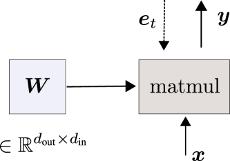
Figure 1: The primal form of a linear layer to be contrasted with the dual form in Figure 2.

Proposition 1 (Attention/Linear Layer Duality).

Let ${\bm{K}}=({\bm{k}}_{1},...,{\bm{k}}_{T})\in\mathbb{R}^{d_{\text{in}}\times T}$ and ${\bm{V}}=({\bm{v}}_{1},...,{\bm{v}}_{T})\in\mathbb{R}^{d_{\text{out}}\times T}$ denote matrices with $T$ column vectors. The following two systems $S_{1}$ and $S_{2}$ are equivalent:

$S_{1}$ (Linear layer): A system consisting of one weight matrix ${\bm{W}}\in\mathbb{R}^{d_{\text{out}}\times d_{\text{in}}}$ constructed as:

$${\bm{W}}=\sum_{t=1}^{T}{\bm{v}}_{t}\otimes{\bm{k}}_{t}$$ (7)

which transforms input ${\bm{x}}\in\mathbb{R}^{d_{\text{in}}}$ to output $S_{1}({\bm{x}})\in\mathbb{R}^{d_{\text{out}}}$ as:

$$S_{1}({\bm{x}})={\bm{W}}{\bm{x}}$$ (8)

$S_{2}$ (Attention layer): A system consisting of memory storing $T$ key-value pairs $({\bm{k}}_{1},{\bm{v}}_{1}),..,({\bm{k}}_{T},{\bm{v}}_{T})$ which transforms input ${\bm{x}}\in\mathbb{R}^{d_{\text{in}}}$ to output $S_{2}({\bm{x}})\in\mathbb{R}^{d_{\text{out}}}$ as:

$$S_{2}({\bm{x}})=\mathrm{Attention}({\bm{K}},{\bm{V}},{\bm{x}})$$ (9)

Proof.

We have almost shown this already in Eq. 5. Given ${\bm{x}}\in\mathbb{R}^{d_{\text{in}}}$, ${\bm{K}}=({\bm{k}}_{1},...,{\bm{k}}_{T})\in\mathbb{R}^{d_{\text{in}}\times T}$ and ${\bm{V}}=({\bm{v}}_{1},...,{\bm{v}}_{T})\in\mathbb{R}^{d_{\text{out}}\times T}$, by starting from the form of attention shown in Lemma 2.2, we obtain

$$S_{2}({\bm{x}}) =\mathrm{Attention}({\bm{K}},{\bm{V}},{\bm{x}})={\bm{V}}{\bm{K}}^{\intercal}{\bm{x}}$$ (10)

$$=\big{(}\sum_{t=1}^{T}{\bm{v}}_{t}\otimes{\bm{k}}_{t}\big{)}{\bm{x}}={\bm{W}}{\bm{x}}=S_{1}({\bm{x}})\qed$$ (11)

This is essentially a general formulation of calculation used to show the equivalence between linear models and kernel machines in the 1960s (Aizerman et al. (1964); cf. Related Work Sec. 4). We express it for an arbitrary weight matrix constructed as a sum of outer-products, and using the modern language of key-value/attention.

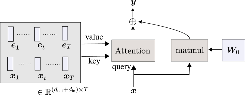
Figure 2: The dual form of a linear layer trained by gradient descent is a key-value memory with attention storing the entire training experience. Compare to the primal form in Figure 1.

3 The Dual Form of Linear Layers in NNs Trained by Gradient Descent

The following corollary obtained from the proposition above is the core result explored in the experimental section. It expresses the dual form of a linear layer trained by gradient descent as a key-value system storing training patterns as key-value pairs, which computes the output from a test query using attention over the key-value memory.

This duality is illustrated in Figures 1 and 2.

Corollary 1 (Dual Form of a Linear Layer Trained by GD).

The following two systems $S_{1}$ and $S_{2}$ are equivalent:

$S_{1}$ (Primal form): A linear layer in a neural network trained by gradient descent in some error function using $T$ training inputs to this layer $({\bm{x}}_{1},...,{\bm{x}}_{T})$ with ${\bm{x}}_{t}\in\mathbb{R}^{d_{\text{in}}}$ and corresponding (backpropagation) error signals $({\bm{e}}_{1},...,{\bm{e}}_{T})$ with ${\bm{e}}_{t}\in\mathbb{R}^{d_{\text{out}}}$ obtained by gradient descent. Its weight matrix ${\bm{W}}\in\mathbb{R}^{d_{\text{out}}\times d_{\text{in}}}$ is thus:

$${\bm{W}}={\bm{W}}_{0}+\sum_{t=1}^{T}{\bm{e}}_{t}\otimes{\bm{x}}_{t}$$ (12)

where ${\bm{W}}_{0}\in\mathbb{R}^{d_{\text{out}}\times d_{\text{in}}}$ is the initialisation. The layer transforms input ${\bm{x}}\in\mathbb{R}^{d_{\text{in}}}$ to output $S_{1}({\bm{x}})\in\mathbb{R}^{d_{\text{out}}}$ as:

$$S_{1}({\bm{x}})={\bm{W}}{\bm{x}}$$ (13)

$S_{2}$ (Dual form): A layer which stores $T$ key-value pairs $({\bm{x}}_{1},{\bm{e}}_{1}),..,({\bm{x}}_{T},{\bm{e}}_{T})$ i.e., a key matrix ${\bm{X}}=({\bm{x}}_{1},...,{\bm{x}}_{T})\in\mathbb{R}^{d_{\text{in}}\times T}$ and a value matrix ${\bm{E}}=({\bm{e}}_{1},...,{\bm{e}}_{T})\in\mathbb{R}^{d_{\text{out}}\times T}$, and a weight matrix ${\bm{W}}_{0}\in\mathbb{R}^{d_{\text{out}}\times d_{\text{in}}}$ which transforms input ${\bm{x}}\in\mathbb{R}^{d_{\text{in}}}$ to output $S_{2}({\bm{x}})\in\mathbb{R}^{d_{\text{out}}}$ as:

$$S_{2}({\bm{x}})={\bm{W}}_{0}{\bm{x}}+\mathrm{Attention}({\bm{X}},{\bm{E}},{\bm{x}})$$ (14)

Proof.

The result is trivially obtained by applying Proposition 1 to $\mathrm{Attention}({\bm{X}},{\bm{E}},{\bm{x}})$ in Eq. 14. ∎

We note that unlike the primal form, the computational complexity of the dual form $S_{2}$ above depends on the number of training datapoints $T$ the layer is trained on (i.e., the number of all inputs forwarded to the linear layer during training for which the loss is computed; that is, in a typical mini-batch stochastic gradient descent setting, the batch size times the number of training iterations). The time and space complexities of the $\mathrm{Attention}$ computation in Eq. 14 is linear in $T$, while $T$ can be potentially very large. The model size is especially prohibitive in practical scenarios: the parameters of the dual form are the ($d_{\text{out}}\times d_{\text{in}}$)-dimensional initial weight matrix ${\bm{W}}_{0}$ —whose size already equals the number of parameters in the primal form— and the $((d_{\text{in}}+d_{\text{out}})\times T)$-sized key-value memory recording all training datapoints. The dual form is thus not a practical form for regular settings. Indeed, this duality of Proposition 1 has been used in the converse direction to obtain time and space efficient attention computation (see Sec. 4/Linear Transformers).

However, there are also benefits in viewing NNs under the dual form. It explicitly shows that the output of an NN linear layer trained by backpropagation is mainly a linear combination of the training error signals ${\bm{e}}_{t}$ the layer receives during training: $\sum_{1}^{T}\alpha_{t}{\bm{e}}_{t}$, where the weights $\alpha_{t}$ are computed by comparing the test query to each training input. This is potentially more interpretable than the primal form as the attention weights $\alpha_{t}=x_{t}^{\intercal}x$ should indicate which training datapoints are “activated” for a given test input. The main contribution of this paper is to effectively implement this dual form and visualise the corresponding attention in different scenarios in Sec. 5. Eq. 14 reveals further notable properties listed as remarks as follows:

Remark 3.1 (Nothing is “forgotten”).

In a system expressed as in the dual form $S_{2}$ of Corollary 1, nothing is forgotten. The entire life of an NN is recorded and stored as a key matrix ${\bm{X}}$ and value matrix ${\bm{E}}$. Roughly speaking, the only limitation of the model’s capability to “remember” something is the limitation of the retrieval process (we illustrate this in the continual learning experiments in Sec. 5.4). Also, note that the $\mathrm{Attention}$ computation in Eq. 14 remains invariant if we shuffle the order of columns in the key-value storage, as it is carried out without any explicit positional encoding (similarly to auto-regressive attention (Irie et al., 2019; Tsai et al., 2019) in some Transformer language models). The time information is naturally encoded into the key and value vectors (except for the key vector in the first layer) tracking the recurrence of the training process in time.

Remark 3.2 (Unlimited memory size is not necessarily useful).

This duality also illustrates an important fact (which might seem counter-intuitive at first glance) that systems which store everything in memory by increasing its size for each new event ($S_{2}$) are not necessarily better than those with a fixed size storage ($S_{1}$). The retrieval mechanism has to be powerful enough to exploit the stored memory. Potentially, we might obtain better models by using other more powerful kernels (e.g., softmax, like in the standard Transformers) in the $\mathrm{Attention}$ computation in Eq. 14. That would, however, require to use the dual form even during training, which is prohibitive.

Remark 3.3 (Orthogonal Inputs).

If an input ${\bm{x}}$ was orthogonal to all training input patterns, the output of the linear layer would be ${\bm{W}}_{0}{\bm{x}}$ (as $\mathrm{Attention}({\bm{X}},{\bm{E}},{\bm{x}})=0$ in Eq. 14), i.e., the weights learned by gradient descent would not contribute to the output.

Remark 3.4 (Non-Uniqueness).

The expression of a linear layer as an attention system is not unique. Some tensor product decompositions can be applied to a trained weight matrix to obtain a more compact attention system. A clear benefit of the one presented in Corollary 1, however, is that it explicitly relates test inputs to training datapoints.

Remark 3.5 (Self-Attention as Two Level Retrieval).

Since this duality is valid for any linear layer trained by gradient descent, and such a linear layer is ubiquitous in any NN, viewing a well known NN architecture from this view could give extra insights and interpretation. For example, the main transformation in a common self-attention (Vaswani et al., 2017) is a linear projection layer which transforms the input to key/value/query vectors. Under the dual form, this can be viewed as a hierarchical retrieval layer where the projection layer conducts a first level of retrieval using unnormalised dot attention on the training datapoints. The second, regular softmax attention conducts a second level of retrieval among those selected by the first level.

4 Related Work

Relating Kernel Machines and NNs.

As stated in Sec. 1, the theoretical results we show in Sec. 2 and 3 are special cases or trivial extensions of the lines of works connecting kernel machines and neural networks derived and presented in different contexts. Most importantly, it is well known that the perceptron (Rosenblatt, 1958) has primal and dual forms as pointed out by Aizerman et al. (1964). The corresponding result is often presented in the case where the co-domain of the linear layer is one-dimensional (i.e., the weight matrix reduces to a weight vector), especially in the literature on support vector and kernel machines (Boser et al., 1992; Burges, 1998) and in textbooks (Schölkopf & Smola, 2002; Bishop, 2006). In Sec. 3, we present the result in the case of linear layers with matrix weights and expressed it in the form of key-value memory which is particularly relevant today (Vaswani et al., 2017). But we note that the same statement could be made using the language of kernel machines as the unnormalised dot attention operation can be expressed as:

$$\mathrm{Attention}({\bm{X}},{\bm{A}},{\bm{x}})+{\bm{b}}=\sum_{t=1}^{T}{\bm{a}}_{t}K({\bm{x}}_{t},{\bm{x}})+{\bm{b}}$$ (15)

where $K$ denotes the dot product, ${\bm{a}}_{t}\in\mathbb{R}^{\text{out}}$ and ${\bm{b}}\in\mathbb{R}^{\text{out}}$ are model parameters.

More recent work of Domingos (2020) presents a more general statement: an entire multi-layer perceptron can be approximated by a kernel machine. While this is a powerful theoretical result, practical ways of exploiting it are yet to be investigated. We study instead the dual form of each linear layer in the network which can be obtained without any approximation.

Transformer Feedforward Block as Key-Value Memory.

Another related but different line of works studies the feedforward block of Transformers as a key-value memory. This feedforward block consists of two feedforward layers which transform input vector ${\bm{x}}\in\mathbb{R}^{d_{\text{in}}}$ as follows:

$$\mathrm{FFN}({\bm{x}})={\bm{W}}_{2}\mathrm{relu}({\bm{W}}_{1}{\bm{x}})$$ (16)

with weight matrices ${\bm{W}}_{1}\in\mathbb{R}^{d_{\text{ff}}\times d_{\text{in}}}$ and ${\bm{W}}_{2}\in\mathbb{R}^{d_{\text{in}}\times d_{\text{ff}}}$, where $d_{\text{ff}}$ denotes the inner dimension (we omit the biases). The possibility to interpret this block as a key-value memory with attention has been pointed out by the original authors of Transformers (Vaswani et al., 2017). Essentially, replacing relu by a softmax,

$${\bm{W}}_{2}\mathrm{softmax}({\bm{W}}_{1}{\bm{x}})$$ (17)

or in our context by removing relu, we can write it down using unnormalised attention defined by Definition 2.1 as:

$${\bm{W}}_{2}{\bm{W}}_{1}{\bm{x}}=\mathrm{Attention}({\bm{W}}_{1}^{\intercal},{\bm{W}}_{2},{\bm{x}})$$ (18)

Using this formulation, Sukhbaatar et al. (2019) proposed to merge the feedforward block and the attention layer by extending the context-dependent key/value vectors in the regular self-attention with a fixed set of trainable key/value vectors. More recently, Geva et al. (2021) asked the question what information from the training data these key vectors (i.e., rows of ${\bm{W}}_{1}$) contain. They compare the corresponding keys to activation vectors of training examples, which are obtained by computing the forward pass of the already trained model on the training examples to be analysed. They conduct such analyses for Transformer language models.

The view we explore here is different. Our statement is not limited to Transformer feedforward blocks, but to any linear layers trained by gradient descent, and we directly express a linear layer as a function of the training datapoints.

Attention and Kernels.

A number of recent works connect attention and kernels (Tsai et al., 2019; Katharopoulos et al., 2020; Choromanski et al., 2021; Peng et al., 2021). While we also implicitly exploit the corresponding connection (Eq. 15), our focus is on connecting the primal form, i.e., linear layers trained by gradient descent, to key-value/attention systems.

Fast Weight Programmers and Linear Transformers.

As we noted while discussing the complexity of the dual form in Sec. 3, the conversion from the primal to the dual form of a linear layer we explore here (Proposition 1) is used in prior works connecting Transformers with linearised attention and fast weight programmers (Ba et al., 2016; Katharopoulos et al., 2020; Schlag et al., 2021). Ba et al. (2016) show the equivalence of unnormalised attention to fast weight programmers of the ’90s (Schmidhuber, 1993). Katharopoulos et al. (2020) convert the self-attention in Transformers—whose complexity is quadratic in sequence length—to a linear-complexity linear layer with fast weights (Schmidhuber, 1991).

5 Experiments

We posit that the dual formulation of linear layers (Corollary 1) offers a possibility to visualise how different training datapoints (i.e., a set of input/error signal pairs seen during training) contribute to some NN’s test time predictions. Here we experimentally support this claim. We effectively study NNs in their dual form and conduct analyses based on the attention weights and related metrics described below. We consider three different scenarios: single-task training, multi-task joint training, and multi-task continual training for image classification using feedforward NNs with two hidden layers. We also conduct experiments with language modelling using a one-layer LSTM recurrent NN.

5.1 Common Settings

We first describe settings which are common to all our experiments. Since our primary interest is to analyse attention weights of Eq. 14 which are simply dot products between a test query ${\bm{x}}$ and each of the training keys ${\bm{x}}_{t}$, the general idea is to train an NN on a given dataset by backpropagation as usual, while recording all inputs to each linear layer during training. After training, attention weights for the trained model for any test example for all training datapoints can be computed by forwarding the test example to the model, to obtain the input vector (test query) to each linear layer, then, we compute the corresponding dot products with the stored training inputs (training keys). We note that the training procedure does not change.

Since storing the inputs to each linear layer for the entire training experience can be highly demanding in terms of disk space, we work with small datasets: MNIST (LeCun et al., 1998) and Fashion-MNIST (Xiao et al., 2017) for image classification, WikiText-2 (Merity et al., 2017) and a small public domain book for language modelling. This allows for obtaining well-performing models with small size within a reasonably small number of training steps.

Our model for image classification has two hidden layers with 800 nodes, each using relu activation functions after each layer. This means that the model has three linear layers which we denote as layer-0, layer-1, and layer-2. The first layer-0 transforms a gray-scale input image of size 768 (28$\times$28) to a 800-dimensional hidden state, layer-1 transforms it to another 800-dimensional hidden state, and finally layer-2 projects it to a 10-dimensional output. The total storage of training patterns is thus roughly 3$\times$800$\times T$ units, where $T$ is the “number of training datapoints” counting all examples across all training mini-batches. We train this model using the vanilla stochastic gradient descent optimiser. We specify relevant metrics in the respective sections below. Many more examples with visualisation are shown in Appendix B.

(a) MNIST class 6

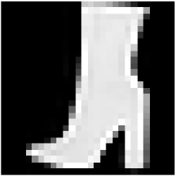
(b) F-MNIST class 9

Figure 3: Test examples used in Figures 4 & 5 (single task case) and Figures 6 & 7 (multi-task joint training case), respectively.

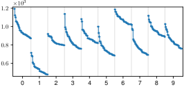
(a) layer-0

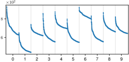
(b) layer-1

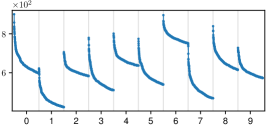
(c) layer-2

Figure 4: Attention weights over training examples for the input test example from class 6 (Figure 3a) for the single task case on MNIST. The x-axis is partitioned by class, and for each class, top-500 datapoints sorted in descending order are shown.

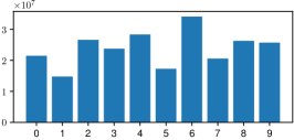
(a) layer-0

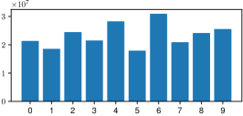
(b) layer-1

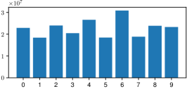
(c) layer-2

Figure 5: Total scores per class for the input test example from class 6 (Figure 3a) for the single task case on MNIST.

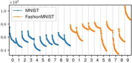
(a) layer-0

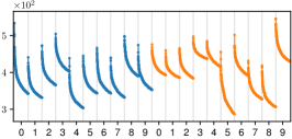
(b) layer-1

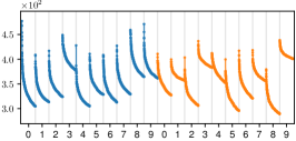
(c) layer-2

Figure 6: Attention weights over training examples for the input test example from class 9 of F-MNIST (Figure 3b) in the joint training case. The x-axis is partitioned by class (for each task), and for each class, top-500 datapoints sorted in descending order are shown.

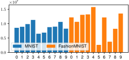
(a) layer-0

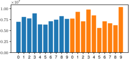
(b) layer-1

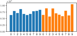
(c) layer-2

Figure 7: Total scores per class for the input test example from class 9 of F-MNIST (Figure 3b) in the joint training case.

5.2 Single Task Case

We start with the simple setting of image classification where we train the two-hidden layer feedforward NN described above on the MNIST dataset (LeCun et al., 1998). This first analysis also serves as the base case for introducing the general idea and key metrics of our study. The model is trained for 3 K updates using a batch size of 128 which correspond to 384 K-long training key/value memory slots. The resulting model achieves 97% accuracy on the test set.

The first plots we visualise are the attention weight “distribution” over training datapoints shown in Figures 4a-4c. The test sample fed to the model in this example is from class 6 (which is digit “6”), shown in Figure 3a, which is correctly classified by the model. In these plots, datapoints are grouped by target class, and for each class, datapoints achieving the top-500 highest scores are shown in descending order (thus, a total of 5 K datapoints out of 384 K are shown) for each layer. While the scores are unnormalised, these plots yield a qualitative picture of the attention “distributions” over classes on the level of datapoints.

However, this picture showing only the top-few-percent datapoints does not capture how much of the attention weights go to which class in total. In fact, in many cases, we notice that the training datapoints which get the highest scores are not necessarily from the correct class (as these top scores may quickly decrease with the rank), while the model’s output prediction is correct. For instance, in the example shown in Figures 4a-4c, the input is an image from class 6 of MNIST (Figure 3a). We indeed see that training examples corresponding to class 6 are attended with high weights in all layers, but we also see that some of the datapoints for class 0 achieve comparable or higher scores than those from the correct class 6. The corresponding top scoring examples are visualised in Figures 10a-10f in Appendix A which contain images from class 0. In order to visualise the total attention weights assigned to each class, we present Figures 5a-5c which show the sum of attention scores per class. Here we observe that training datapoints from the correct class label 6 are the most attended datapoints overall. By examining multiple cases, we observe that the sum of attention weights effectively correlates well with the model output. To quantify this observation, we compute the corresponding correlation on the entire test set. Table 1 shows the results. We observe that when the model’s prediction is correct, the total attention weights correlate well with the model output, especially in the late layers.

Table 1: Prediction accuracy (%) of the true target label (Target) and model output (Output) from argmax of the per-class attention scores (like those in Figure 5), shown for each layer for two cases whether the model’s output prediction is correct. Mean and standard deviation computed for 5 runs. Layer-0 is the input layer.

		Is Model Prediction Correct?
Layer		No	Yes
0	Target	17.2 $\pm$ 2.7	75.1 $\pm$ 0.0
	Output	49.5 $\pm$ 1.5
1	Target	18.0 $\pm$ 2.9	78.8 $\pm$ 0.8
	Output	52.9 $\pm$ 2.9
2	Target	20.6 $\pm$ 2.6	84.7 $\pm$ 1.1
	Output	60.1 $\pm$ 4.5

As a side note, we also considered an alternative version where we augment the attention weights with the norm of the error vector (value vector in Eq. 14). However, the resulting plots did not show any consistent trend (presumably because the norm disregards the signs of each component of error/value vectors). In fact, in general, the heatmap of attention weights (e.g., Vaswani et al. (2017); Bahdanau et al. (2015)) often reported in the literature also completely disregards any information about the value vectors. Our analysis is thus also purely based on attention weights, i.e., interaction between a test query and training key vectors.

Regarding the time information in layer-1 and layer-2 (it does not matter in the input layer-0, since it is simply a dot product between the raw images which contains no such information), we find the distribution over time to be rather spread out and noisy among the top-500 highest scoring datapoints. We do not observe a clear pattern indicating that the most recent training datapoints are more important.

5.3 Multi-Task Case

Now we extend the experimental setting above by training models with the same architecture as above, but jointly on two datasets: MNIST and Fashion-MNIST (F-MINST for short). The output dimension remains 10. The model is trained for 5,000 steps and achieves 97% and 87% test accuracy on MNIST and F-MNIST, respectively.

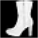
(a) layer-0, top-1

(b) layer-1, top-1

(c) layer-1, top-2

(d) layer-2, top-2

(e) layer-2, top-3

Figure 11: Top matching training examples. for the input test example from class 9 of F-MNIST (Figure 3b) in the joint training case.

In case of joint training, a natural question to ask is how the attention behaves with two datasets and how much cross-task attention occurs (i.e., high attention scores when key and query are from different datasets). Intuitively, since the output representation is shared (labels between 0 and 9), representations learned by the late layers might be task-independent, and cross-task attention might take place. We experimentally observe that this is indeed the case. Figures 6a-6c show the attention weights over training datapoints in the case of joint training, analogous to Figures 4a-4c for the single task case. The x-axis now shows 20 groups representing 10 classes from MNIST and 10 from F-MNIST. Figure 3b shows the test example fed to the model which is from class 9 of F-MINST (“ankle boot”). On Figures 6a-6c, we observe that, while in layer-0, top matching training datapoint are dominated by F-MNIST datapoints from the same class, in layer-1 and layer-2, top attention weights are more distributed across two tasks. Especially in layer-2, the top-3 matching examples (shown in Figures 11a-11e in Appendix A) contain datapoints from MNIST, one of them belonging to class 9. Analogous to the single task case, Figures 7a-7c show the sum of weights for each class (separately for each dataset). Another interesting observation: while the class achieving the highest total attention scores in layer-0 is class 4 (“coat”) of F-MNIST (computed as a dot product between the raw images), in later layers, the score of the correct label 9 is increased, which is not surprising if we expect the late layers to yield better representations of inputs. This is a visual illustration of the results we saw in Table 1 where the argmax of the sum of attention weights correlates better with the model output in the late layers.

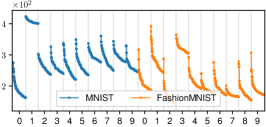
(a) layer-0

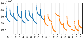
(b) layer-1

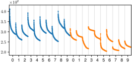
(c) layer-2

Figure 8: Plots analogous to Figure 6 for the input test example from class 1 of MNIST (Figure 12d) in the continual learning case.

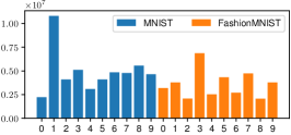
(a) layer-0

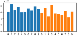
(b) layer-1

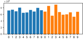
(c) layer-2

Figure 9: Total scores per class for the input test example from class 1 of MNIST (Figure 12d) in the continual training case.

5.4 Continual Learning Case

Finally we train models on the two datasets successively in a continual learning fashion, first on MNIST for 3,000 steps, then on F-MINST for 3,000 steps. The final test accuracies are 85% on F-MNIST and 45% on MNIST (down from 97% after training on MNIST only).

The continual learning case is particularly interesting from the perspective of the dual form. Since all training patterns are stored in the training key/value memory (Eq. 14), if we used an attention mask on the F-MNIST part of training keys for the attention computation, the model would be able to reproduce the good performance on MNIST obtained after the first part of training, and thus avoid degradation or more generally catastrophic forgetting (French, 1999). But there is no such a mask in practice: using an MNIST test input, we observe strong attention weights on the F-MNIST part of training patterns, causing severe interference.

In Figures 8 and 9, we present an illustrative example which shows how an MNIST test image clearly representing the digit “1” (shown in Figure 12d in Appendix B) is wrongly recognised as “3” through interference of F-MNIST class 3 (see an example in Figure 12e) which is “dress”. In the attention maps in Figure 9a, we observe that the MNIST class 1 training examples are highly activated, so are the class 3 of F-MNIST. As we move up to layer-1 and layer-2 (Figures 9b and 9c), the attention becomes more distributed across two tasks, and we finally observe that in layer-2 (Figure 9c), the class 3 of F-MNIST becomes the most dominant class, which may explain the model’s decision to output class 3. Otherwise, when the test input is from F-MNIST, we observe trends similar to the one reported for the joint training case in Sec. 5.3. Examples for the correctly classified cases can be found in Appendix B.3.

5.5 Language Modelling

The experiments above focus on image data and feedforward NNs. Here we conduct experiments with texts using a recurrent NN (RNN). A desirable NLP experiment would be to train a big Transformer language model (LM) on a vast amount of data, and analyse the attention of linear layers over the training datapoints while sampling from the model. As we can not afford such a gigantic experiment, we train a one-layer LSTM LM on two small datasets: a tiny public domain book, “Aesop’s Fables”, by J. H. Stickney and the standard WikiText-2 dataset (Merity et al., 2017). The basic approach is similar to the one we introduced above: we train LMs as usual, while recording inputs to each linear layer. Here we focus on the linear layer in the LSTM layer (i.e., the single linear transformation which groups all projections including all transformations for the gates). At test time, we forward the trained LM on a prompt (short text segment) and get the test query from the last token from the prompt. We compute the attention weights for all (token-level) training datapoints. Since it is difficult to visualise attention “distribution” over different token positions in the entire training tokens in a comprehensive manner, we visualise the text segment around the training datapoints achieving the highest attention weights (we sum all attention weights which go to the same training token position).

Table 2 shows an example from the word-level WikiText-2 experiment. The test query is from a passage in the Wikipedia page on a warship. We observe that the training passages achieving the highest attention scores are also from pages about warships, and they have a similar sentence structure. A manual inspection shows that the passage with a similar sentence structure but on an unrelated topic (singer) is not attended, which indicates that the attention here is contextual. We refer to Appendix C for more examples, details, and character-level experiments. While the scale is limited, we found all examples interesting and intuitive. They may be capturing the essence of how bigger models could be “attending” to different parts of training texts based on some common concept defined by the test query.

Table 2: Example test query and top-3 training passages (with their Wikipedia page title) from WikiText-2. We also show a manually found negative example (which is not among the top scoring passages but has a similar sentence structure). The test query token and the top scoring training token are highlighted in bold. The query is from the test text. We refer to Appendix C for more examples.

Query (Ironclad warship)	… Her principal role was for combat in the English Channel and other European …
Top-1 (Portuguese ironclad)	Her sailing rig also was removed . Her main battery guns were replaced with new …
Top-2 (SMS Markgraf)	… between the two funnels . Her secondary armament consisted of fourteen 15 cm …
Top-3 (Italian cruiser Aretusa)	single mounts . Her primary offensive weapon was her five 450 mm.
Negative (Nina Simone)	… written especially for the singer . Her first hit song in America was her rendition …

6 Discussion and Limitations

The dual formulation allows for explicitly visualising attention weights over all training patterns, given a test input. While we argue that this view provides a new perspective on analysing neural networks, it also has several limitations. First, the memory storage requirement forces us to conduct experiments with small datasets (see more discussion in Appendix D). On the other hand, storage requirements grow linearly with training set size, while computing hardware is still getting exponentially cheaper with time. That is, soon we may be able to analyse much larger models trained on much larger datasets. Second, our analysis is not applicable to models which are already trained. Furthermore, it is limited to a study of attention weights, in line with traditional visualisations of attention-based systems, and can only show which training datapoints are combined. It does not tell how the combined representations can be converted to a meaningful output, e.g., in the case of large generative NNs mentioned in the introduction.

7 Conclusion

We revisit the dual form of the perceptron for linear layers in deep NNs. The dual form is expressed in terms of the now popular key/value/attention concepts, which offers novel insights and interpretability. We visualise and study the corresponding attention weights. This allows for connecting training datapoints to test time predictions, and observing many interesting patterns in various scenarios, on both image and language modalities. While our analysis is still limited to relatively small datasets, it opens up new avenues for analysing and interpreting behaviours of deep NNs.

Appendix A Top Matching Examples

This section contains figures of images in the training set achieving the highest attention scores (top-3) in each layer in the single task and multi-task joint training cases. We refer to these examples in the main text in Sec. 5.2 and 5.3. We note that one example from class 0 (Figure 10a) is often found in the top-3 matches in different settings we study, presumably as the corresponding image of digit “0” highly overlaps with other images in the original image space.

(a) layer-0, top-1

(b) layer-1, top-1

(c) layer-1, top-2

(d) layer-2, top-1

(e) layer-2, top-2

(f) layer-2, top-3

Figure 10: Top matching training examples for the input test example from class 6 (Figure 3a) in the single task case on MNIST.

Appendix B More Examples/Visualisation

Here we provide more examples that do not fit the space limitations of the main text. All input test examples used to generate figures in the appendix are summarised in Figure 12. We refer to each of them in the subsections below.

(a) MNIST, 3

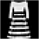
(b) F-MNIST, 3 (dress)

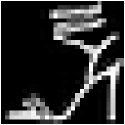
(c) F-MNIST, 5 (sandal)

(d) MNIST, 1

(e) F-MNIST, 3 (dress)

(f) MNIST, 7

Figure 12: Input test examples used for various scenarios studied in this appendix.

B.1 Single Task Case

Here we simply show one more example in the single task case discussed in Sec. 5.2. The input test example used here is shown in Figure 12a (digit “3”). The plots of attention weights and the corresponding sums per class are show in Figures 14 and 15. The observations are similar to those discussed in Sec. 5.2. The training examples achieving the highest attention scores in each layer are shown in Figure 13.

(a) layer-0 top-1

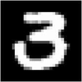
(b) layer-0 top-2

(c) layer-0 top-3

(d) layer-1 top-1

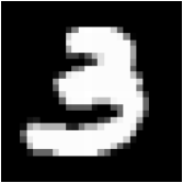
(e) layer-1 top-2

(f) layer-1 top-3

(g) layer-2 top-1

(h) layer-2 top-2

(i) layer-2 top-3

Figure 13: Top scoring examples for the MNIST input of Figure 12a in the single task case.

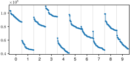
(a) layer-0

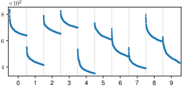
(b) layer-1

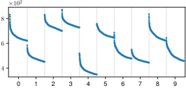
(c) layer-2

Figure 14: Attention weights over training examples for the input test example from class 3 of MNIST (Figure 12a) in the single task case. x-axis is partitioned by class, and for each class, top-500 datapoints sorted in descending order are shown.

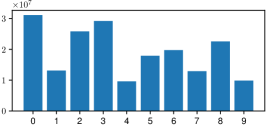
(a) layer-0

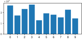
(b) layer-1

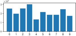
(c) layer-2

Figure 15: Total scores per class, for the input test example from class 3 of MNIST (Figure 12a) in the single task case.

B.2 Joint Training Case

Here we show two more examples for the multi-task joint training case discussed in Sec. 5.3. The input test examples used here are shown in Figure 12b (class 3 “dress”) and 12c (class 5 “sandal”). Both of them are correctly classified by the model. The training examples achieving the highest attention scores in each layer are shown in Figures 16 and 19, respectively. The plots of the attention weights and the corresponding sums per class are shown in Figures 17 and 18 for the class 3 input, and in Figures 20 and 21 for the class 5 input. In the first example (F-MNIST, class 3), we do not see MNIST examples among the top scoring training examples (see Figure 16), unlike in the second case (F-MNIST, class 5) where we do see the digit “5” of MNIST (see Figure 19). The second example also illustrates the case where the argmax of the sum disagrees with the model decision (illustrating the limitations of analysis based on attention weights only, see Sec. 6).

(a) layer-0 top-1

(b) layer-0 top-2

(c) layer-0 top-3

(d) layer-1 top-1

(e) layer-1 top-2

(f) layer-1 top-3

(g) layer-2 top-1

(h) layer-2 top-2

(i) layer-2 top-3

Figure 16: Top scoring examples for the F-MNIST input of Figure 12b in the joint training case.

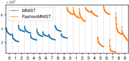
(a) layer-0

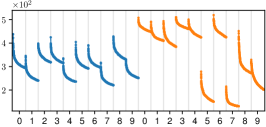
(b) layer-1

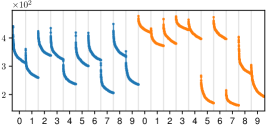
(c) layer-2

Figure 17: Attention weights over training examples for the input test example from class 3 of F-MNIST (Figure 12b) in the joint training case. The x-axis is partitioned by class, and for each class, top-500 datapoints sorted in descending order are shown.

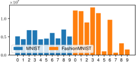
(a) layer-0

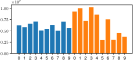
(b) layer-1

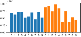
(c) layer-2

Figure 18: Total scores per class for the input test example from class 3 of F-MNIST (Figure 12b) in the joint training case.

(a) layer-0 top-1

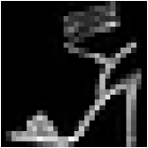
(b) layer-0 top-2

(c) layer-0 top-3

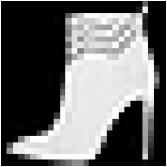
(d) layer-1 top-1

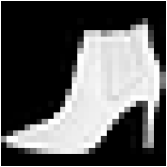
(e) layer-1 top-2

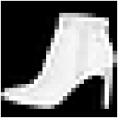
(f) layer-1 top-3

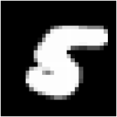
(g) layer-2 top-1

(h) layer-2 top-2

(i) layer-2 top-3

Figure 19: Top scoring examples for the F-MNIST input of Figure 12c in the joint training case.

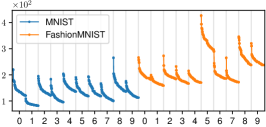
(a) layer-0

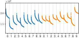
(b) layer-1

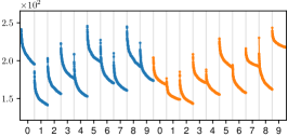
(c) layer-2

Figure 20: Attention weights over training examples for the input test example from class 5 of F-MNIST (Figure 12c) in the joint training case. The x-axis is partitioned by class, and for each class, top-500 datapoints sorted in descending order are shown.

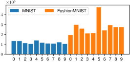
(a) layer-0

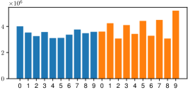
(b) layer-1

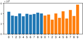
(c) layer-2

Figure 21: Total scores per class for the input test example from class 5 of F-MNIST (Figure 12c) in the joint training case.

B.3 Continual Learning Case

In the continual learning case, we show three examples: one MNIST example (Figure 12d) which is misclassified, and two others which are correctly classified (one from MNIST is shown in Figure 12f, one from F-MNIST in Figure 12e).

The misclassified example (Figures 8 and 9) has been already discussed in Sec. 5.4.

For the correctly classified inputs, Figures 27 and 28 respectively show the attention weights and the sums for the MNIST input (Figure 12f) of class 7, and Figures 24 and 25 show them for the F-MNIST input (Figure 12e) of class 3 (“dress”).

The training examples achieving the highest attention scores in each case are shown in Figures 22, 23, and 26.

(a) layer-0 top-1

(b) layer-0 top-2

(c) layer-0 top-3

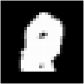
(d) layer-1 top-1

(e) layer-1 top-2

(f) layer-1 top-3

(g) layer-2 top-1

(h) layer-2 top-2

(i) layer-2 top-3

Figure 22: Top scoring examples for the misclassified MNIST input of Figure 12d in the continual training case.

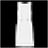
(a) layer-0 top-1

(b) layer-0 top-2

(c) layer-0 top-3

(d) layer-1 top-1

(e) layer-1 top-2

(f) layer-1 top-3

(g) layer-2 top-1

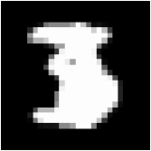
(h) layer-2 top-2

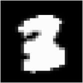
(i) layer-2 top-3

Figure 23: Top scoring examples for the correctly classified F-MNIST input of Figure 12e in the continual training case.

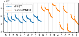
(a) layer-0

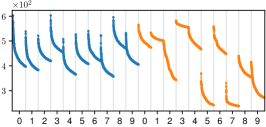
(b) layer-1

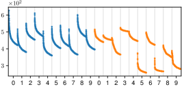
(c) layer-2

Figure 24: Attention weights over training examples for the input test example from class 3 of F-MNIST (Figure 12e) in the continual training case. The x-axis is partitioned by class, and for each class, top-500 datapoints sorted in descending order are shown.

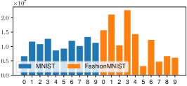
(a) layer-0

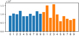
(b) layer-1

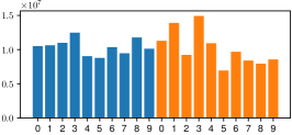
(c) layer-2

Figure 25: Total scores per class for the input test example from class 3 of F-MNIST (Figure 12e) in the joint training case.

(a) layer-0 top-1

(b) layer-0 top-2

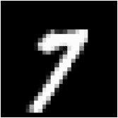
(c) layer-0 top-3

(d) layer-1 top-1

(e) layer-1 top-2

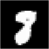
(f) layer-1 top-3

(g) layer-2 top-1

(h) layer-2 top-2

(i) layer-2 top-3

Figure 26: Top scoring examples for the correctly classified MNIST input of Figure 12f in the continual training case.

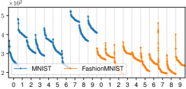
(a) layer-0

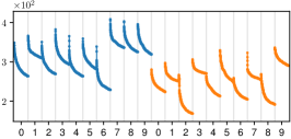
(b) layer-1

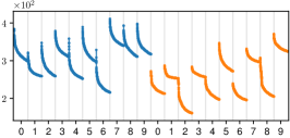
(c) layer-2

Figure 27: Attention weights over training examples for the input test example from class 7 of MNIST (Figure 12f) in the continual training case. The x-axis is partitioned by class, and for each class, top-500 datapoints sorted in descending order are shown.

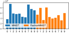
(a) layer-0

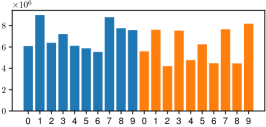
(b) layer-1

(c) layer-2

Figure 28: Total scores per class for the input test example from class 7 of MNIST (Figure 12f) in the continual training case.

Appendix C Language Modelling Experiments

C.1 Basic Settings

Here we describe experimental details of our language modelling experiments introduced in Sec.5.5 and provide more examples.

We train a one-layer LSTM language model (LM) on two small datasets: a tiny public domain book, “Aesop’s Fables”, by J. H. Stickney (publicly available under the project Gutenberg) and the standard WikiText-2 dataset (Merity et al., 2017).

We train a word-level LM on WikiText-2 (about 2 M running words) and a character-level LM on the book (about 185 K running characters). The word-level model has a vocabulary size of 33 K, and the input word embedding and the LSTM dimension of 200. For the character-level LM, the vocabulary size is 107, with an input embedding size of 64 and an LSTM layer of size 1024. For Aesop’s Fables, we isolated the last parts of the book (containing alternative versions of the tales) as a test set to generate test queries. For WikiText-2, we use the regular train/valid/test splits.

As has been mentioned in Sec.5.5, we focus on analysing the linear layer in the LSTM RNN layer (i.e. the single linear transformation which groups all projections including all transformations for the gates). The input to this linear layer consists of one input coming from the previous layer and the LSTM state from the previous time step.

Please find the corresponding analysis for the character-level LM on Aesop’s Fables in Sec. C.2, and for the word-level LM on WikiText-2 in Sec. C.3. Generally, we found all examples interesting and intuitive.

C.2 Character-Level Experiments on “Aesop’s Fables”

Tables 3, 4 and 5 show the queries we used and the corresponding top scoring training text passages for Aesop’s Fables.

Table 3: Example test query and top-3 training passages from Aesop’s Fables. The test query token and the top scoring training token are highlighted in bold. The query text is taken from the test set. We see training examples with a concept of “doing something fast” getting high attention scores.

Query	… Wolf was glad to take himself off as fast as his legs would carry him. …
Top-1	When the Hare awoke, the Tortoise was not in sight; and running as fast
	as he could, he found her comfortably dozing at their goal.
Top-2	But the Stork with his long legs easily followed them to the water,
	and kept on eating them as fast as he could.
Top-3	The poor Mule made room for him as fast as he could, and the Horse went proudly on his way.

Table 4: Example test query and top-3 training passages from Aesop’s Fables. The test query token and the top scoring training token are highlighted in bold. The query text is taken from the test set. We see training examples with a phrase of form “a + adjective/single + word starting with d” getting high attention scores.

Query	The Wolf stood high up the stream and the Lamb a little distance below.
Top-1	when the Pigeons had let him come in, they found that
	he slew more of them in a single day than the Kite could
Top-2	all the advantages that you mention, yet when I hear the
	bark of but a single dog, I faint with terror
Top-3	GREAT Cloud passed rapidly over a country which was
	parched by heat, but did not let fall a single drop to refresh it.

Table 5: Example test query and top-3 training passages from Aesop’s Fables. The test query token and the top scoring training token are highlighted in bold. Here the query is from the training text. We see training examples with a phrase of form “at” plus some timing or counting related concept getting high attention scores.

Query	The Squirrel takes a look at them—he can do no more. At SPACE one time he is called away;
	at another, even dragged off in the Lion’s service.
Top-1	… at seeing an elephant. Is it his great bulk that you so much admire? Mere size is nothing.
	At SPACE most it can only frighten little girls and boys
Top-2	At times he would snap at his prey, and at SPACE times play
	with him and lick him with his tongue, …
Top-3	As the Log did not move, they swam round it, keeping a safe distance away,
	and at SPACE last one by one hopped upon it.

C.3 Word-Level Experiments on WikiText-2

Tables 2, 6 and 7 show the examples for the word-level language model trained on WikiText-2.

Table 6: Example test query and top-3 training passages (with their Wikipedia page title) from WikiText-2. The test query token and the top scoring training token are highlighted in bold. The query is from the test text. We see some training passages about “some contributions of somebody on something” getting high attention scores.

Query	her painting was printed opposite that of Tommy Watson , who was by this time famous ,
(Josepha Petrick Kemarre)	particularly for his contribution to the design of a new building for …
Top-1 (Laurence Olivier)	In February 1960 , for his contribution to the film industry ,
	Olivier was inducted into the Hollywood Walk of Fame
Top-2 (Khoo Kheng-Hor)	he was appointed as honorary Assistant Superintendent of Police by
	the Singapore Police Force in recognition for his contribution as consultant
Top-3 (History of AI)	Colby did not credit Weizenbaum for his contribution to the program .

Appendix D Further Discussion on Scalability

We further discuss the scalability of the analysis introduced here for larger models. The main requirement for the analysis presented here is to store training datapoints during training, whose size linearly increases with the number of training steps. The complexity of test-time attention weight computation is also linear w.r.t. the number of training steps, and it is just a one-time computation, which is nothing compared to the resources needed for training the model. The largest GPT3 model has a state size of 12K and is trained on 300B tokens. The dual form of one self-attention layer would thus require 300G * 12K * 4 = 14PB storage. This is huge, but not infeasible. Alternatively, if the training is reproducible, we could opt for not storing training datapoints: train the model once, compute test queries, then re-train the model to recompute the training datapoints to compute test attention weights and store only the statistics relevant for the analysis (e.g., top-k and sum).

Table 7: Example test query and top-3 training passages (with their Wikipedia page title) from WikiText-2. The test query token and the top scoring training token are highlighted in bold. The query is from the test text. We see training examples about “somebody rating (or commenting on) something (e.g. movie/song)” getting high attention scores.

Query	… IGN ’s Matt gave ” The ” a score of 9 @.@ 4 out of 10 , describing it as ” a …
(The Snowmen)	in storytelling ” which ” refreshingly ” lacked traditional Christmas references
Top-1	Den of Geek writer named it the ” finest ” stand @-@ alone episode of the second season ,
(Irresistible (film))	describing it as ” a genuinely creepy 45 @-@ minute horror movie ” …
Top-2	NME felt that it was the ” most impressive ” song on the album , describing it as a
(Moment of Surrender)	” gorgeously sparse prayer built around Adam Clayton ’s bassline and Bono ’s rough ” …
Top-3 (Species (film))	James from magazine gave the film 2 out of 5 stars , describing it as ” ’ Alien ’ meets …

References

- Aizerman et al. (1964) Aizerman, M. A., Braverman, E. M., and Rozonoer, L. I. Theoretical foundations of potential function method in pattern recognition. Automation and Remote Control, 25(6):917–936, 1964.
- Ba et al. (2016) Ba, J., Hinton, G. E., Mnih, V., Leibo, J. Z., and Ionescu, C. Using fast weights to attend to the recent past. In Proc. Advances in Neural Information Processing Systems (NIPS), pp. 4331–4339, Barcelona, Spain, December 2016.
- Bahdanau et al. (2015) Bahdanau, D., Cho, K., and Bengio, Y. Neural machine translation by jointly learning to align and translate. In Int. Conf. on Learning Representations (ICLR), San Diego, CA, USA, May 2015.
- Balestriero et al. (2021) Balestriero, R., Pesenti, J., and LeCun, Y. Learning in high dimension always amounts to extrapolation. Preprint arXiv:2110.09485, 2021.
- Bishop (2006) Bishop, C. M. Pattern Recognition and Machine Learning. Springer, 2006.
- Boser et al. (1992) Boser, B. E., Guyon, I., and Vapnik, V. A training algorithm for optimal margin classifiers. In Proc. Annual ACM Conference on Computational Learning Theory (COLT), pp. 144–152, Pittsburgh, PA, USA, July 1992. ACM.
- Brown et al. (2020) Brown, T. B. et al. Language models are few-shot learners. In Proc. Advances in Neural Information Processing Systems (NeurIPS), Virtual only, December 2020.
- Burges (1998) Burges, C. J. A tutorial on support vector machines for pattern recognition. Data mining and knowledge discovery, 2(2):121–167, 1998.
- Choromanski et al. (2021) Choromanski, K., Likhosherstov, V., Dohan, D., Song, X., Gane, A., Sarlos, T., Hawkins, P., Davis, J., Mohiuddin, A., Kaiser, L., et al. Rethinking attention with performers. In Int. Conf. on Learning Representations (ICLR), Virtual only, 2021.
- Domingos (2020) Domingos, P. Every model learned by gradient descent is approximately a kernel machine. Preprint arXiv:2012.00152, 2020.
- French (1999) French, R. M. Catastrophic forgetting in connectionist networks. Trends in cognitive sciences, 3(4):128–135, 1999.
- Geva et al. (2021) Geva, M., Schuster, R., Berant, J., and Levy, O. Transformer feed-forward layers are key-value memories. In Proc. Conf. on Empirical Methods in Natural Language Processing (EMNLP), pp. 5484–5495, Online and Punta Cana, Dominican Republic, November 2021.
- Graves (2008) Graves, A. Supervised sequence labelling with recurrent neural networks. PhD thesis, Technical University Munich, 2008.
- Graves et al. (2014) Graves, A., Wayne, G., and Danihelka, I. Neural turing machines. Preprint arXiv:1410.5401, 2014.
- Hochreiter & Schmidhuber (1997) Hochreiter, S. and Schmidhuber, J. Long short-term memory. Neural computation, 9(8):1735–1780, 1997.
- Irie et al. (2019) Irie, K., Zeyer, A., Schlüter, R., and Ney, H. Language modeling with deep Transformers. In Proc. Interspeech, pp. 3905–3909, Graz, Austria, September 2019.
- Katharopoulos et al. (2020) Katharopoulos, A., Vyas, A., Pappas, N., and Fleuret, F. Transformers are RNNs: Fast autoregressive transformers with linear attention. In Proc. Int. Conf. on Machine Learning (ICML), Virtual only, July 2020.
- Krizhevsky (2009) Krizhevsky, A. Learning multiple layers of features from tiny images. Master’s thesis, Computer Science Department, University of Toronto, 2009.
- LeCun et al. (1998) LeCun, Y., Cortes, C., and Burges, C. J. The MNIST database of handwritten digits. URL http://yann. lecun. com/exdb/mnist, 1998.
- Luong et al. (2015) Luong, M.-T., Pham, H., and Manning, C. D. Effective approaches to attention-based neural machine translation. In Proc. Conf. on Empirical Methods in Natural Language Processing (EMNLP), pp. 1412–1421, Lisbon, Portugal, September 2015.
- Merity et al. (2017) Merity, S., Xiong, C., Bradbury, J., and Socher, R. Pointer sentinel mixture models. In Int. Conf. on Learning Representations (ICLR), Toulon, France, April 2017.
- Mikolov et al. (2013) Mikolov, T., Sutskever, I., Chen, K., Corrado, G. S., and Dean, J. Distributed representations of words and phrases and their compositionality. In Proc. Advances in Neural Information Processing Systems (NIPS), pp. 3111–3119, Lake Tahoe, NV, USA, September 2013.
- Miller et al. (2016) Miller, A. H., Fisch, A., Dodge, J., Karimi, A., Bordes, A., and Weston, J. Key-value memory networks for directly reading documents. In Proc. Conf. on Empirical Methods in Natural Language Processing (EMNLP), pp. 1400–1409, Austin, TX, USA, November 2016.
- Peng et al. (2021) Peng, H., Pappas, N., Yogatama, D., Schwartz, R., Smith, N. A., and Kong, L. Random feature attention. In Int. Conf. on Learning Representations (ICLR), Virtual only, 2021.
- Ramesh et al. (2021) Ramesh, A., Pavlov, M., Goh, G., Gray, S., Voss, C., Radford, A., Chen, M., and Sutskever, I. Zero-shot text-to-image generation. In Proc. Int. Conf. on Machine Learning (ICML), pp. 8821–8831, Virtual only, July 2021.
- Rosenblatt (1958) Rosenblatt, F. The perceptron: a probabilistic model for information storage and organization in the brain. Psychological review, 65(6):386, 1958.
- Schlag et al. (2021) Schlag, I., Irie, K., and Schmidhuber, J. Linear Transformers are secretly fast weight programmers. In Proc. Int. Conf. on Machine Learning (ICML), Virtual only, July 2021.
- Schmidhuber (1991) Schmidhuber, J. Learning to control fast-weight memories: An alternative to recurrent nets. Technical Report FKI-147-91, Institut für Informatik, Technische Universität München, March 1991.
- Schmidhuber (1993) Schmidhuber, J. Reducing the ratio between learning complexity and number of time varying variables in fully recurrent nets. In International Conference on Artificial Neural Networks (ICANN), pp. 460–463, Amsterdam, Netherlands, September 1993.
- Schölkopf & Smola (2002) Schölkopf, B. and Smola, A. J. Learning with kernels: support vector machines, regularization, optimization, and beyond. MIT press, 2002.
- Sukhbaatar et al. (2015) Sukhbaatar, S., Szlam, A., Weston, J., and Fergus, R. End-to-end memory networks. In Proc. Advances in Neural Information Processing Systems (NIPS), pp. 2440–2448, Montréal, Canada, December 2015.
- Sukhbaatar et al. (2019) Sukhbaatar, S., Grave, E., Lample, G., Jegou, H., and Joulin, A. Augmenting self-attention with persistent memory. Preprint arXiv:1907.01470, 2019.
- Tsai et al. (2019) Tsai, Y.-H. H., Bai, S., Yamada, M., Morency, L.-P., and Salakhutdinov, R. Transformer dissection: An unified understanding for transformer’s attention via the lens of kernel. In Proc. Conf. on Empirical Methods in Natural Language Processing (EMNLP), pp. 4344–4353, Hong Kong, China, November 2019.
- Vaswani et al. (2017) Vaswani, A., Shazeer, N., Parmar, N., Uszkoreit, J., Jones, L., Gomez, A. N., Kaiser, Ł., and Polosukhin, I. Attention is all you need. In Proc. Advances in Neural Information Processing Systems (NIPS), pp. 5998–6008, Long Beach, CA, USA, December 2017.
- Xiao et al. (2017) Xiao, H., Rasul, K., and Vollgraf, R. Fashion-MNIST: a novel image dataset for benchmarking machine learning algorithms. Preprint arXiv:1708.07747, 2017.
- Zeiler & Fergus (2014) Zeiler, M. D. and Fergus, R. Visualizing and understanding convolutional networks. In Proc. European Conf. on Computer Vision (ECCV), volume 8689, pp. 818–833, Zurich, Switzerland, September 2014.