Answer Set Planning: A Survey

Abstract

Answer Set Planning refers to the use of Answer Set Programming (ASP) to compute plans, i.e., solutions to planning problems, that transform a given state of the world to another state. The development of efficient and scalable answer set solvers has provided a significant boost to the development of ASP-based planning systems. This paper surveys the progress made during the last two and a half decades in the area of answer set planning, from its foundations to its use in challenging planning domains. The survey explores the advantages and disadvantages of answer set planning. It also discusses typical applications of answer set planning and presents a set of challenges for future research.

1 Introduction

Automated planning represents one of the core components in the design of autonomous intelligent systems. The term refers to the task of finding a course of actions (i.e., a plan) that changes the state of the world from a given state to another state. An automated planner takes a planning problem as input, which consists of a domain description or an action theory, the initial state description, and the goal state description, and computes a solution of the problem if one exists. Automated planning has been an active research area of Artificial Intelligence for many years. It has established itself as a mature research area with its own annually conference, the International Conference on Automated Planning and Scheduling (ICAPS) series starting from 1991, with several satellite workshops related to planning and scheduling as well as the planning competition for many tracks. Consequently, the literature on planning is enormous. The textbooks by ghallabnt04 and 2016 includes more than 500 and 600 references, respectively. The monograph on planning with focus on abstraction and decomposition by Yang (1997) has more than 150 references. The survey on classical planning by Hendler et al. (1990) also referred to more than 100 papers. Similar observation can be made about the survey by Weld (1994), which mainly discusses partial order planning. There are also special collections or special issues on planning such as Allen et al. (1991, 1990). In addition, several planning systems addressing different aspects of planning have been developed, which will be discussed in more details in Sections 3–5. Our goal in this paper is to provide a survey on answer set planning, a relatively late addition to the rich body of research in automated planning that has not been comprehensively surveyed so far.

Answer set planning, a term coined by Lifschitz (1999), refers to the use of Answer Set Programming (ASP) in planning. In this approach, planning problems are translated to logic programs whose answer sets correspond to solutions of the original planning problems. This approach is related to the early approach to planning using automated theorem provers by Green (1969). Although similar in the emphasis of using a general logical solver for planning, answer set planning and planning using automated theorem provers differ in that the former computes an answer set (or a full model) to find a solution whilst the latter identifies a solution with a proof of a query. Answer set planning is more closely related to the prominent approach of planning using satisfiability solvers (SAT-planning) proposed by Kautz and Selman (1992) and Kautz et al. (1996), who showed, experimentally, that SAT-planning can reach the scalability and efficiency of contemporary heuristic-based planning systems. This success is, likely, one of the driving forces behind the research on using logic programs under the answer set semantics for planning. The idea of answer set planning was first discussed by Subrahmanian and Zaniolo (1995) and further developed by Dimopoulos et al. (1997), who also demonstrated that answer set planning can be competitive with state-of-the-art domain-independent planner at the time.

Answer set planning offers a number of features which are advantageous for researchers. First, by virtue of the declarative nature of logic programming, answer set planning is itself declarative and elaboration tolerant. This enables a modular development of planning systems with special features. For example, to consider a particular set of solutions satisfying an user’s preferences, one only needs to develop rules expressing these preferences and adds them to the set of rules encoding the planning problem Son and Pontelli (2006); to exploit the various types of domain-knowledge in planning, one only needs to develop rules expressing them to the set of rules encoding the planning problem Son et al. (2006). To the best of our knowledge, there exists no other planning system that can simultaneously exploit all three well-known types of domain knowledge—temporal, hierarchical, and procedural knowledge—as demonstrated by Son et al. (2006). Other features of logic programming such as the use of variables, constraints, and choice atoms allow for a compact representation of answer set planners. For example, the basic code for generating a plan in classical setting requires only 10 basic rules and one constraint while a traditional implementation of a planning system in an imperative language may require thousands of lines. Second, the expressiveness of logic programming facilitates the integration of complex reasoning, such as reasoning with static causal laws, into ASP-based planners. To the best of our knowledge, only answer set planning systems deal directly with unrestricted static causal laws Son et al. (2005a); Tu et al. (2011). Third, as demonstrated in several experimental evaluations Gebser et al. (2013); Son et al. (2005a); Tu et al. (2007, 2011), answer set planning systems perform well against other contemporary planning systems in various categories. Finally, the large body of theoretical building block results in logic programming supports the development of provably correct answer set planners. This is an important feature of answer set planning that is mostly neglected by the vast majority of work in planning, arguably difficult to obtain for planners realized using traditional imperative programming techniques and valuable for foundational research work.

Over the last twenty-five years, a variety of ASP-based planning systems have been developed, e.g. Dimopoulos et al. (2019); Eiter et al. (2000, 2003b); Gebser et al. (2013); Son et al. (2005a); Tu et al. (2007, 2011); Morales et al. (2007); Fandinno et al. (2021); Rizwan et al. (2020); Spies et al. (2019); Yalciner et al. (2017), that address several challenges in planning, such as planning with incomplete information, non-deterministic actions, and sensing actions. These systems, in turn, provide the basis for investigation of ASP solutions to problems in areas like diagnosis Balduccini and Gelfond (2003), multi-agent path findings Nguyen et al. (2017); Gómez et al. (2020), goal recognition design Son et al. (2016), planning with preferences Son and Pontelli (2006), planning with action cost Eiter et al. (2003a), and robot task planning Jiang et al. (2019). This progress has been amplified by the development of efficient and scalable answer set solvers, such as smodels  Niemelä and Simons (1997), dlv Eiter et al. (1997); Alviano et al. (2017); Alviano et al. (2013), clasp Gebser et al. (2007, 2019), and cmodels Lierler and Maratea (2004), together with the invention of action languages for reasoning about actions and change, such as the action languages $\mathcal{A}$, $\mathcal{B}$, and $\mathcal{C}$ Gelfond and Lifschitz (1998), $\mathcal{A}_{K}$ with sensing actions Lobo et al. (1997); Son and Baral (2001), and actions with nondeterminism Giunchiglia et al. (1997).

In this survey, we characterize planning problems using the three dimensions:

1. the type of action theories,

2. the degree of uncertainty about the initial state, and

3. the availability of knowledge-producing actions.

In particular, the literature has named the following classes of planning problems. Classical planning refers to planning problems with deterministic action theories and complete initial states. Conformant planning deals with the incompleteness of the initial state and nondeterministic action theories. Conditional planning considers knowledge producing actions and generates plans which might contain non-sequential constructs, such as if-then or while loop.

This paper presents a survey of research focused on ASP-based planning and its applications. It begins (Section 2) with a brief introduction of answer set programming and action language $\mathcal{B}$, the main representation language for planning problems. It describes different encodings of answer set planning for problems with complete information and no sensing actions (Section 3). The paper then introduces two different approaches to planning with incomplete information (Section 4) and the description of a conditional planner, which solves planning problems in domains with sensing actions and incomplete information (Section 5). The survey explores next the problems of planning with preferences (Section 6), diagnosis (Section 7), planning in multi-agent environments (Section 8), and planning and scheduling in real-world applications (Section 9). The paper concludes with a discussion about open challenges for answer set planning (Section 10).

2 Background

2.1 Answer Set Programming

As usual, a logic program consists of rules of the form

$$a_{1}\vee\ldots\vee a_{m}\leftarrow a_{m+},\dots,a_{n},{not\>}a_{n+1},\dots,{not\>}a_{o}$$

where each $a_{i}$ is an atom of form $p(t_{1},\dots,t_{k})$ and all $t_{i}$ are terms, composed of function symbols and variables. Atoms $a_{1}$ to $a_{m}$ are often called head atom, while $a_{m+1}$ to $a_{n}$ and ${not\>}a_{n+1}$ to ${not\>}a_{o}$ are also referred to as positive and negative body literals, respectively. An expression is said to be ground, if it contains no variables. As usual, ${not\>}$ denotes (default) negation. A rule is called a fact if $m=o=1$, normal if $m=1$, and an integrity constraint if $m=0$. Semantically, a logic program produces a set of stable models, also called answers sets, which are distinguished models of the program determined by the stable model semantics; see the paper by Gelfond and Lifschitz (1991) for details.

To ease the use of ASP in practice, several simplifying notations and extensions have been developed. First of all, rules with variables are viewed as shorthands for the set of their ground instances. Additional language constructs include conditional literals and cardinality constraints Simons et al. (2002). The former are of the form $a:{b_{1},\dots,b_{m}}$, the latter can be written as $s\{d_{1};\dots;d_{n}\}t$, where $a$ and $b_{i}$ are possibly default-negated (regular) literals and each $d_{j}$ is a conditional literal; $s$ and $t$ provide optional lower and upper bounds on the number of satisfied literals in the cardinality constraint. We refer to $b_{1},\dots,b_{m}$ as a condition. The practical value of both constructs becomes apparent when used with variables. For instance, a conditional literal like $a(X):b(X)$ in a rule’s antecedent expands to the conjunction of all instances of $a(X)$ for which the corresponding instance of $b(X)$ holds. Similarly, $2\;\{a(X):b(X)\}\;4$ is true whenever at least two and at most four instances of $a(X)$ (subject to $b(X)$) are true. Finally, objective functions minimizing the sum of a set of weighted tuples $(w_{i},\boldsymbol{t}_{i})$ subject to condition $c_{i}$ are expressed as $\#minimize\{w_{1}@l_{1},\boldsymbol{t}_{1}:c_{1};\dots;w_{n}@l_{n},\boldsymbol{t}_{n}:c_{n}\}$. Analogously, objective functions can be optimized using the $\#\textit{maximize}$ statement. Lexicographically ordered objective functions are (optionally) distinguished via levels indicated by $l_{i}$. An omitted level defaults to 0. Furthermore, $w_{i}$ is a numeral constant and $\boldsymbol{t}_{i}$ a sequence of arbitrary terms. Alternatively, the above minimize statement can be expressed by weak constraints of the form $\hookleftarrow c_{i}[w_{i}@l_{i},\boldsymbol{t}_{i}]$ for $1\leq i\leq n$.

As an example, consider the following rule:

$$1\{\mathit{move}(D,P,T):\mathit{disk}(D),\mathit{peg}(P)\}1\leftarrow\mathit{ngoal}(T-1),T\leq n.$$

This rule has a single head atom consisting of a cardinality constraint; it comprises all instances of $\mathit{move}(D,P,T)$ where $T$ is fixed by the two body literals and $D$ and $P$ vary over all instantiations of predicates $\mathit{disk}$ and $\mathit{peg}$, respectively. Given 3 pegs and 4 disks, this results in 12 instances of $\mathit{move}(D,P,T)$ for each valid replacement of $\mathit{T}$, among which exactly one must be chosen according to the above rule.

Full details of the input language of clingo, along with various examples and its semantics, can be found in the papers by  Gebser et al. (2015). The interested reader is also referred to the work by Calimeri et al. (2019) for the description of the ASP Core 2 Language.

A logic program can have zero, one, or multiple answer sets. This distinguishes answer set semantics from other semantics of logic programs such as the well-founded semantics of Van Gelder et al. (1991) or perfect models semantics of Przymusinski (1988). Answer set semantics, together with the introduction of choice rules and constraints, enables the development of answer set programming as proposed by Lifschitz (1999). Following this approach, a problem can be solved by a logic program whose answer sets correspond one-to-one to the problem’s solutions. Choice rules are often used to generate potential solutions and constraints are used to eliminate potential but incorrect solutions.

2.2 Reasoning About Actions: The Action Description Language $\mathcal{B}$

We review the basics of the action description language $\mathcal{B}$ Gelfond and Lifschitz (1998). An action theory in $\mathcal{B}$ is defined over a set of actions A and a set of fluents F. A fluent literal is a fluent $f\in\mathbf{F}$ or its negation $\neg f$. A fluent formula is a Boolean formula constructed from fluent literals. An action theory is a set of laws of the form

$$\hbox{\bf caused}(\varphi,f)$$ (1)

$$\hbox{\bf causes}(a,f,\varphi)$$ (2)

$$\hbox{\bf executable}(a,\varphi)$$ (3)

$$\hbox{\bf initially}(f)$$ (4)

where $f$ and $\varphi$ are a fluent literal and a set of fluent literals, respectively, and $a$ is an action. A law of the form (1) represents a static causal law, i.e., a relationship between fluents. It conveys that whenever the fluent literals in $\varphi$ hold then so is $f$. A dynamic causal law is of the form (2) and represents the (conditional) effect of $a$ while a law of the form (3) encodes an executability condition of $a$. Intuitively, an executability condition of the form (3) states that $a$ can only be executed if $\varphi$ holds. A dynamic law of the form (2) states that $f$ is caused to be true after the execution of $a$ in any state of the world where $\varphi$ holds. When $\varphi=\emptyset$ in (3), we often omit laws of this type from the theory. Statements of the form (4) describe the initial state. They state that $f$ holds in the initial state. We also often refer to $\varphi$ as the “precondition” for each particular law.

An action theory is a pair $(D,\Gamma)$ where $\Gamma$, called the initial state, consists of laws of the form (4) and $D$, called the domain, consists of laws of the form (1)-(3). For convenience, we sometimes denote the set of laws of the form (1) by $D_{C}$.

Example 1

Let us consider a modified version of the suitcase $s$ with two latches from the work by Lin (1995). We have a suitcase with two latches $l_{1}$ and $l_{2}$. $l_{1}$ is up and $l_{2}$ is down. To open a latch ($l_{1}$ or $l_{2}$), we need a corresponding key ($k_{1}$ or $k_{2}$, respectively). When the two latches are in the up position, the suitcase is unlocked. When one of the latches is down, the suitcase is locked. In this domain, we have that

$$\mathbf{A}=\{open(l_{i}),close(l_{i}),get\_key(k_{i})\mid i\in\{1,2\}\}$$

and

$$\mathbf{F}=\{locked\}\cup\{up(l_{i}),holding(k_{i})\mid i\in\{1,2\}\}.$$

The intuitive meaning of the actions and fluents is clear. The problem can be represented using the laws

$$D^{s}=\left\{\begin{array}[]{ll}\hbox{\bf causes}(open(l_{i}),up(l_{i}),\emptyset)&\\ \hbox{\bf causes}(close(l_{i}),\neg up(l_{i}),\emptyset)&\\ \hbox{\bf causes}(get\_key(k_{i}),holding(k_{i}),\emptyset)&\\ \hbox{\bf executable}(open(l_{i}),\{holding(k_{i})\})&\\ \hbox{\bf caused}(\{\neg up(l_{i})\},locked)&\\ \hbox{\bf caused}(\{up(l_{1}),up(l_{2})\},\neg locked)&\\ \end{array}\right.$$

where, in all laws, $i=1,2$. The first three laws describe the effects of the action of opening a latch, closing a latch, or getting a key. The fourth law encodes that we can open the latch only when we have the right key. Observe that the omission of executability laws for $close(l_{i})$ or $get\_key(k_{i})$ indicates that these actions can always be executed. The last two laws are static causal laws encoding that the suitcase is locked when either of the two latches is in the down position and it is unlocked when the two latches are in the up position.

A possible initial state of this domain is given by

$$\Gamma^{s}=\left\{\begin{array}[]{lllll}\hbox{\bf initially}(up(l_{1}))\\ \hbox{\bf initially}(\neg up(l_{2}))\\ \hbox{\bf initially}(locked)\\ \hbox{\bf initially}(\neg holding(k_{1}))\\ \hbox{\bf initially}(holding(k_{2}))\\ \end{array}\right.$$

$\diamond$

A domain given in $\mathcal{B}$ defines a transition function from pairs of actions and states to sets of states whose precise definition is given below. Intuitively, given an action $a$ and a state $s$, the transition function $\Phi$ defines the set of states $\Phi(a,s)$ that may be reached after executing the action $a$ in state $s$. The mapping to a set of states captures the fact that an action can potentially be non-deterministic and produce different results (e.g., an action open might be successful in opening a lock or not if we account for the possibility of a broken lock). If $\Phi(a,s)$ is an empty set it means that the execution of $a$ in $s$ is undefined. We now formally define $\Phi$.

Let $D$ be a domain in $\mathcal{B}$. A set of fluent literals is said to be consistent if it does not contain $f$ and $\neg f$ for some fluent $f$. An interpretation $I$ of the fluents in $D$ is a maximal consistent set of fluent literals of $D$. A fluent $f$ is said to be true (resp. false) in $I$ if $f\in I$ (resp. $\neg f\in I$). The truth value of a fluent formula in $I$ is defined recursively over the propositional connectives in the usual way. For example, $f\wedge g$ is true in $I$ if $f$ is true in $I$ and $g$ is true in $I$. We say that a formula $\varphi$ holds in $I$ (or $I$ satisfies $\varphi$), denoted by $I\models\varphi$, if $\varphi$ is true in $I$.

Let $u$ be a consistent set of fluent literals and $K$ a set of static causal laws. We say that $u$ is closed under $K$ if for every static causal law

$$\hbox{\bf caused}(\varphi,f)$$

in $K$, if $u\models\bigwedge_{p\in\varphi}p$ then $u\models f$. By $Cl_{K}(u)$ we denote the least consistent set of literals from $D$ that contains $u$ and is also closed under $K$. It is worth noting that $Cl_{K}(u)$ might be undefined when it is inconsistent. For instance, if $u$ contains both $f$ and $\neg f$ for some fluent $f$, then $Cl_{K}(u)$ cannot contain $u$ and be consistent; another example is that if $u=\{f,g\}$ and $K$ contains

$$\hbox{\bf caused}(\{f\},h)\quad\quad\textnormal{ and }\quad\quad\hbox{\bf caused}(\{f,g\},\neg h),$$

then $Cl_{K}(u)$ does not exist because it has to contain both $h$ and $\neg h$, which means that it is inconsistent.

Formally, a state of $D$ is an interpretation of the fluents in F that is closed under the set of static causal laws $D_{C}$ of $D$.

An action $a$ is executable in a state $s$ if there exists an executability proposition

$$\hbox{\bf executable}(a,\varphi)$$

in $D$ such that $s\models\bigwedge_{p\in\varphi}p$. Clearly, if $\varphi=\emptyset$, then $a$ is executable in every state of $D$.

The direct effect of an action a in a state $s$ is the set

$$e(a,s)=\left\{f\mid\hbox{\bf causes}(a,f,\varphi)\in D,s\models\bigwedge_{\textstyle{p\in\varphi}}p\right\}.$$

For a domain $D$, the set of states $\Phi(a,s)$ that may be reached by executing $a$ in $s$, is defined as follows.

1. If $a$ is executable in $s$, then

   $$\Phi(a,s)=\{s^{\prime}\mid s^{\prime}\mbox{ is a state and }s^{\prime}=Cl_{D_{C}}(e(a,s)\cup(s\cap s^{\prime}))\};$$

2. If $a$ is not executable in $s$, then $\Phi(a,s)=\emptyset$.

Intuitively, the states produced by $\Phi(a,s)$ are fixpoints of an equation, obtained by closing (with respect to all static causal laws) the set which includes the direct effects $e(a,s)$ of action $a$ and the fluents whose value does not change as we transition from $s$ to $s^{\prime}$ through action $a$ (i.e., $s\cap s^{\prime}$).

The presence of static causal laws introduces non-determinism to action theories, i.e., $\Phi(a,s)$ can contain more than one element. For instance, consider the theory with the set of laws

$$\{\hbox{\bf causes}(a,f),\quad\hbox{\bf caused}(\{f,\neg g\},\neg h),\quad\hbox{\bf caused}(\{f,\neg h\},\neg g)\}.$$

It is easy to check that

$$\Phi(a,\{\neg f,\neg g,\neg h\})=\{\{f,g,\neg h\},\{f,\neg g,h\}\}.$$

Every domain $D$ in $\mathcal{B}$ has a unique transition function $\Phi$, and we say $\Phi$ is the transition function of $D$. We illustrate the definition of the transition function in the next example.

Example 2

For the suitcase domain in Example 1, the initial state, given by the set of laws $\Gamma^{s}$, is defined by

$$s_{0}=\{up(l_{1}),\neg up(l_{2}),locked,\neg holding(k_{1}),holding(k_{2})\}.$$

In state $s_{0}$, the three actions $open(l_{2})$, $close(l_{1})$, and $close(l_{2})$ are executable. $open(l_{2})$ is executable since $holding(k_{2})$ is true in $s_{0}$ while $close(l_{1})$ and $close(l_{2})$ are executable since the theory (implicitly) contains the laws

$$\hbox{\bf executable}(close(l_{1}),\{\})\hskip 28.45274pt\textnormal{ and }\hskip 28.45274pt\hbox{\bf executable}(close(l_{2}),\{\})$$

which indicate that these two actions are always executable. The following transitions are possible from state $s_{0}$:

$$\{\>up(l_{1}),up(l_{2}),\neg locked,\neg holding(k_{1}),holding(k_{2})\>\} \in \Phi(open(l_{2}),s_{0}).$$

$$\{\>up(l_{1}),\neg up(l_{2}),locked,\neg holding(k_{1}),holding(k_{2})\>\} \in \Phi(close(l_{2}),s_{0}).$$

$$\{\>\neg up(l_{1}),\neg up(l_{2}),locked,\neg holding(k_{1}),holding(k_{2})\>\} \in \Phi(close(l_{1}),s_{0}).$$

$\diamond$

The transition function $\Phi$ is extended to define $\widehat{\Phi}$ for reasoning about effects of action sequences in the usual way. For a sequence of actions $\alpha=\langle a_{0},\ldots,a_{n-1}\rangle$ and a state $s$, $\widehat{\Phi}(\alpha,s)$ is a collection of states defined as follows:

• $\widehat{\Phi}(\alpha,s)=\{s\}$ if $\alpha=\langle\ \rangle$;

• $\widehat{\Phi}(\alpha,s)=\Phi(a_{0},s)$ if $n=1$;

• $\widehat{\Phi}(\alpha,s)=\bigcup_{s^{\prime}\in\Phi(a_{0},s)}\widehat{\Phi}(\alpha^{\prime},s^{\prime})$ if $n>1$, $\Phi(a_{0},s)\neq\emptyset$, and $\widehat{\Phi}(\alpha^{\prime},s^{\prime})\neq\emptyset$ for every $s^{\prime}\in\Phi(a_{0},s)$ where $\alpha^{\prime}=\langle a_{1},\ldots,a_{n-1}\rangle$.

A domain $D$ is consistent if for every action $a$ and state $s$, if $a$ is executable in $s$, then $\Phi(a,s)\neq\emptyset$. An action theory $(D,\Gamma)$ is consistent if $D$ is consistent and $s_{0}=\{f\mid\hbox{\bf initially}(f)\in\Gamma\}$ is a state of $D$. In what follows, we consider only consistent action theories and refer to $s_{0}$ as the initial state of $D$. We call a sequence of alternate states and actions $s_{0}a_{0}\ldots a_{k-1}s_{k}$ a trajectory if $s_{i+1}\in\Phi(a,s_{i})$ for every $i=0,\ldots,k-1$.

A planning problem with respect to $\mathcal{B}$ is specified by a triple $\langle D,\Gamma,\Delta\rangle$ where $(D,\Gamma)$ is an action theory in $\mathcal{B}$ and $\Delta$ is a set of fluent literals (or goal). A sequence of actions $\alpha=\langle a_{0},\ldots,a_{n-1}\rangle$ is then called an optimistic plan for $\Delta$ if there exists some $s\in\widehat{\Phi}(\alpha,s_{0})$ such that $s\models\Delta$ where $s_{0}$ is the initial state of $D$. Note that we use the term ‘optimistic plan’ to refer to $\alpha$, as used by Eiter et al. (2003b), instead of ‘plan’ because the non-determinicity of $D$ does not guarantee that the goal is achieved in every state reachable after the execution of $\alpha$. However, if $D$ is deterministic, i.e., $|\Phi(a,s)|\leq 1$ for every pair $(a,s)$ of actions and states, then the two notions of ‘optimistic plan’ and ‘plan’ coincide.

3 Planning with Complete Information

Given a planning problem $\mathcal{P}=\langle D,\Gamma,\Delta\rangle$, answer set planning solves it by translating it into a logic program $\Pi(\mathcal{P},n)$ whose answer sets correspond one-to-one to optimistic plans of length $\leq n$ of $\mathcal{P}$. Intuitively, each answer set corresponds to a trajectory $s_{0}a_{0}\ldots a_{n-1}s_{n}$ such that $s_{n}\models\Delta$. As such, the choices that need to be made at each step $k$ in program $\Pi(\mathcal{P},n)$ are either the action $a_{k}$ or the state $s_{k}$. This leads to different encodings, referred to as action-based and state-based, which emphasize the object of the selection process.

Over the years, several types of encodings have been developed. We present below two of the most popular mappings of planning problems to logic programs. The first encoding, presented in Subsection 3.1, views the problem $\mathcal{P}$ as a set of laws in the language $\mathcal{B}$ (Subsection 2.2) while the second encoding, illustrated in Subsection 3.2, views the problem as a set of facts. In both encodings, the program $\Pi(\mathcal{P},n)$ contains the atom $time(0..n)$ to represent the set of facts $\{time(0),\ldots,time(n)\}$.

3.1 A Direct Encoding

The rules of $\Pi(\mathcal{P},n)$ in this encoding are described by Son et al. (2006). The main predicates in the program are:

1. $holds(F,T)$ – the fluent literal $F$ is true at time step $T$;

2. $occ(A,T)$ – the action $A$ occurs at time step $T$; and

3. $possible(A,T)$ – the action $A$ is executable at time step $T$.

The program contains two sets of rules. The first set of rules is domain dependent. The rules in the second set are generic and common to all problems. For a set of literals $\varphi$, we use $holds(\varphi,T)$ to denote the set $\{holds(L,T)\mid L\in\varphi\}$.

3.1.1 Domain-Dependent Rules

For each planning problem $\mathcal{P}=\langle D,\Gamma,\Delta\rangle$, program $\Pi(\mathcal{P},n)$ contains the following rules:

1. For each element $\hbox{\bf initially}(f)$ of form (4) in $\Gamma$, the fact

   $$holds(f,0)\leftarrow$$ (5)

   stating that the fluent literal $f$ holds at time step $0$.

2. For each executability condition $\hbox{\bf executable}(a,\varphi)$ of form (3) in $D$, the rule

   $$possible(a,T)\leftarrow time(T),holds(\varphi,T)$$ (6)

   stating that it is possible to execute the action $a$ at time step $T$ if $\varphi$ holds at time step $T$.

3. For each dynamic causal law $\hbox{\bf causes}(a,f,\varphi)$ of form (2) in $D$, the rule

   $$\begin{array}[]{lll}holds(f,T+1)&\leftarrow&time(T),occ(a,T),holds(\varphi,T)\end{array}$$ (7)

   stating that if $a$ occurs at time step $T$ then the fluent literal $f$ becomes true at $T+1$ if the conditions in $\varphi$ hold.

4. For each static causal law $\hbox{\bf caused}(\varphi,f)$ of form (1) in $D$, the rule

   $$holds(f,T)\leftarrow time(T),holds(\varphi,T)$$ (8)

   which represents a straightforward translation of the static causal law into a logic programming rule.

5. To guarantee that an action is executed only when it is executable, the constraint

   $$\leftarrow time(T),occ(A,T),{not\>}possible(A,T)$$ (9)

We demonstrate the above translation by listing the set of domain dependent rules for the domain from Example 1.

Example 3

Besides the set of facts encoding actions and fluents and the initial state (for each $a\in\mathbf{A}$, $f\in\mathbf{F}$ and $\hbox{\bf initially}(l)\in\Gamma^{s}$),

$$action(a)\leftarrow\hskip 56.9055ptfluent(f)\leftarrow\hskip 56.9055ptholds(l,0)\leftarrow$$

the encoding of the suitcase domain in Example 1 contains the following rules for $i=1,2$:

$$\begin{array}[]{lll}holds(up(l_{i}),T+1)&\leftarrow&time(T),occ(open(l_{i}),T)\\ holds(\neg up(l_{i}),T+1)&\leftarrow&time(T),occ(close(l_{i}),T)\\ holds(holding(k_{i}),T+1)&\leftarrow&time(T),occ(get\_key(k_{i}),T)\\ possible(open(l_{i}),T)&\leftarrow&time(T),holds(holding(k_{i}),T)\\ holds(locked,T)&\leftarrow&time(T),holds(\neg up(l_{i}),T)\\ holds(\neg locked,T)&\leftarrow&time(T),holds(up(l_{1}),T),holds(up(l_{2}),T)\\ possible(close(l_{i}),T)&\leftarrow&time(T)\\ possible(get\_key(k_{i}),T)&\leftarrow&time(T)\\ \end{array}$$

Each of the first six rules corresponds to a law in $D^{s}$. The last two rules are added because there is no restriction on the executability condition of $close(l_{i})$ or $get\_key(k_{i})$. $\Diamond$

3.1.2 Domain Independent Rules

The set of domain independent rules of $\Pi(\mathcal{P},n)$ consists of rules for generating action occurrences and encoding the frame axiom.

1. Action generation rule: To create plans, $\Pi(\mathcal{P},n)$ must contain rules that generate action occurrences of the form $occ(a,t)$. This is encoded by the rule

   $$1\{occ(A,T):action(A)\}1\leftarrow time(T),T<n$$ (10)

   stating that exactly one action must occur at each time step. It makes use of the cardinality atom $1\{occ(A,T):action(A)\}1$ which is true for a time step $T$ iff exactly one atom in the set $\{occ(A,T):action(A)\}$ is true. The former atom can be replaced by $l\{occ(A,T):action(A)\}u$ where $0\leq l\leq u$ to allow for different types of plans, e.g., for parallel plans, $l>1$.

2. Inertia rule: The frame axiom, which states that a property continues to hold unless it is changed, is encoded as follows:

   $$holds(F,T{+}1) \leftarrow time(T),fluent(F),holds(F,T),{not\>}holds(\neg F,T{+}1)\quad\quad$$ (11)

   $$holds(\neg F,T{+}1) \leftarrow time(T),fluent(F),holds(\neg F,T),{not\>}holds(F,T{+}1)$$ (12)

3. Consistency constraint: To ensure that states encoded by answer sets are consistent, $\Pi(\mathcal{P},n)$ contains the following constraint:

   $$\leftarrow fluent(F),holds(F,T),holds(\neg F,T)$$ (13)

   Observe that this constraint is needed because $holds(f,t)$ and $holds(\neg f,t)$ are “consistent” for answer set solvers. It would not be needed if $holds(\neg f,t)$ is encoded as $\neg holds(f,t)$.

3.1.3 Goal Representation

The goal $\Delta$ is encoded by rules defining the predicate $goal$, which is true whenever $\Delta$ is true, and a rule that enforces that $\Delta$ must be true at time step $n$. For example, if $\Delta$ is a conjunction of literals $p_{1}\wedge\ldots\wedge p_{k}$, then the rules

$$goal \leftarrow holds(p_{1},n),\ldots,holds(p_{k},n)$$ (14)

$$\leftarrow {not\>}goal$$ (15)

encode $\Delta$ and enforce that $\Delta$ must be true at time step $n$.

3.1.4 Correctness of the Encoding

Let $\mathcal{P}=(D,\Gamma,\Delta)$ and $\Pi(\mathcal{P},n)$ be the logic program consisting of

• the set of facts encoding fluents and literals in $D$;

• the set of domain-dependent rules encoding $D$ and $\Gamma$ (rules (5)–(9)) in which the domain of $T$ is $\{0,\ldots,n\}$;

• the set of domain-independent rules (rules (10)–(12)) in which the domain of $T$ is $\{0,\ldots,n\}$; and

• the rules (13)–(15).

The following result shows the equivalence between optimistic plans achieving $\Delta$ and answer sets of $\Pi(\mathcal{P},n)$. To formalize the theorem, we introduce some additional notation. For an answer set $M$ of $\Pi(\mathcal{P},n)$, we define

$$s_{i}(M)=\{f\ \mid f\textnormal{ is a fluent literal and }holds(f,i)\in M\}.$$

Theorem 1

For a planning problem $\langle D,\Gamma,\Delta\rangle$ with a consistent action theory $(D,\Gamma)$, $s_{0}a_{0}\ldots a_{n-1}s_{n}$ is a trajectory achieving $\Delta$ iff there exists an answer set $M$ of $\Pi(\mathcal{P},n)$ such that

1. $occ(a_{i},i)\in M$ for $i\in\{0,\ldots,n-1\}$ and

2. $s_{i}=s_{i}(M)$ for $i\in\{0,\ldots,n\}$.

Remark 1

1. The proof of Theorem 1 relies on the following observations: $M$ is an answer set of $\Pi(\mathcal{P},n)$ iff

   • for every $i$ such that $0\leq i<n$, there exists some $a_{i}\in\mathbf{A}$ such that

     $occ(a_{i},i)\in M$ and $a_{i}$ is executable in $s_{i}(M)$;

   • $s_{0}(M)$ is the initial state of the action theory $(D,\Gamma)$ and is consistent. Furthermore, for every $i$ such that $0\leq i<n$, $s_{i+1}(M)\in\Phi(a_{i},s_{i}(M))$; and

   • $\Delta$ is true in $s_{n}(M)$.

   The theorem is similar to the correspondence between histories and answer sets explored by Lifschitz and Turner (1999) and by Son et al. (2006).

2. If $(D,\Gamma)$ is deterministic then Theorem 1 can be simplified to “ $a_{0},a_{1},\ldots,a_{n-1}$ is a plan achieving $\Delta$ iff there exists an answer set $M$ of $\Pi(\mathcal{P},n)$ such that $occ(a_{i},i)\in M$ for $i\in\{0,\ldots,n-1\}$.”

3. A different variant of this encoding, which uses $f(\vec{x},t)$ and $\neg f(\vec{x},t)$ instead of $holds(f(\vec{x}),t)$ and $holds(\neg f(\vec{x}),t)$, respectively, can be found in several papers related to answer set planning, e.g., in the papers by Lifschitz (1999) and 2002.

4. The action language $\mathcal{B}$ could be extended with various features such as default fluents, effects of action sequences, etc. as discussed by Gelfond and Lifschitz (1998). These features can be easily included in the encoding of $\Pi(\mathcal{P},n)$. On the other hand, such features are rarely considered in action domains used by the planning community. For this reason, we do not consider such features in this survey.

5. Readers familiar with current answer set solvers such as clingo or dlv could be wondering why $holds(\neg f,t)$ is used instead of a perhaps more intuitive $\neg holds(f,t)$. Indeed, the former can be replaced by the latter. The use of $holds(\neg f,t)$ is influenced by early Prolog programs written for reasoning about actions and changes by Michael Gelfond. A Prolog program that translates a planning problem to its ASP encoding can be found at https://www.cs.nmsu.edu/~tson/ASPlan/Knowledge/translate.pl.

6. Different approaches to integrate various types of knowledge to answer set planning can be found in the work by Dix et al. (2005) and Son et al. (2006).

3.2 Meta Encoding

The meta encoding presented in this section encodes a planning problem $\mathcal{P}=\langle D,\Gamma,\Delta\rangle$ as a set of facts, in addition to a set of domain-independent rules for reasoning about effects of actions. To distinguish this encoding from the previous one, we denote this encoding with $\Pi^{m}(\mathcal{P},n)$. In this encoding, a set $\varphi$ is represented using the atom $set(s_{\varphi})$, where $s_{\varphi}$ is a new atom associated to $\varphi$, and a set of atoms of the form $\{member(s_{\varphi},p)\mid p\in\varphi\}$. The laws in $D$ are represented by the set of facts

$$caused(f,s_{\mathit{sf}}). set(s_{\mathit{sf}}). s_{\mathit{sf}}\textnormal{ is the identifier for }\varphi\textnormal{ in }\hbox{\bf caused}(f,\varphi)\textnormal{ in }D$$ (16)

$$causes(a,f,s_{\mathit{df}}). set(s_{\mathit{df}}). s_{\mathit{df}}\textnormal{ is the identifier for }\varphi\textnormal{ in }\hbox{\bf causes}(a,f,\varphi)\textnormal{ in }D$$ (17)

$$executable(a,s_{a}). set(s_{a}). s_{a}\textnormal{ is the identifier for }\varphi\textnormal{ in }\hbox{\bf executable}(a,\varphi)\textnormal{ in }D$$ (18)

and the set of facts encoding $s_{\mathit{sf}}$, $s_{\mathit{df}}$, and $s_{a}$.

In addition to the action generation rule (10), the inertial rules (11)–(12), the goal representation rules (14)-(15), and the constraint stating that actions can occur only when they are executable (9), the program $\Pi^{m}(\mathcal{P},n)$ contains the following rules for reasoning about effects of actions:

$$holds(S,T) \leftarrow time(T),set(S),$$

$$holds(F,T):fluent(F),member(S,F);$$

$$holds(\neg F,T):fluent(F),member(S,\neg F).$$

$$holds(L,T+1) \leftarrow time(T),causes(A,F,S),occ(A,T),holds(S,T)$$ (20)

$$holds(L,T) \leftarrow time(T),caused(L,S),holds(S,T)$$ (21)

$$possible(A,T) \leftarrow time(T),executable(A,S),holds(S,T)$$ (22)

Rule (3.2) defines the truth of a set of fluents $S$ at time step $T$, by declaring that $S$ holds at $T$ if all of its members are true at $T$. The intuition behind the rules (20)–(22) is clear. Similarly to Theorem 1, answer sets of $\Pi^{m}(\mathcal{P},n)$ correspond one-to-one to possible solutions (optimistic plans) of $\mathcal{P}$.

Remark 2

A similar encoding to $\Pi^{m}(\mathcal{P},n)$ is used in the system plasp version 3 by Dimopoulos et al. (2019). A translation of planning problems from PDDL format to ASP facts can be found at https://github.com/potassco/plasp.

3.3 Adding Heuristics: Going for Performance

By using ASP systems for solving planning problems, we employ general-purpose systems rather than genuine planning systems. In particular, the distinction between action and fluent variables or fluent variables of successive states completely eludes the ASP system. Pioneering work in this direction was done by Rintanen (2012), where the implementation of SAT solvers was modified in order to boost performance of SAT planning. Inspired by this research direction, Gebser et al. (2013) developed a language extension for ASP systems that allows users to declare heuristic modifiers that take effect in the underlying ASP system clingo.

More precisely, a heuristic directive is of form

$$\#\mathit{heuristic}\ a:b_{1},\dots,b_{m}.\,[w,m]$$

where $a$ is an atom and $b_{1},\dots,b_{m}$ is a conjunction of literals; $w$ is a numeral term and $m$ a heuristic modifier, indicating how the solver’s heuristic treatment of $a$ should be changed whenever $b_{1},\dots,b_{m}$ holds. Clingo distinguishes four primitive heuristic modifiers:

init

for initializing the heuristic value of $a$ with $w$,

factor

for amplifying the heuristic value of $a$ by factor $w$,

level

for ranking all atoms; the rank of $a$ is $w$,

sign

for attributing the sign of $w$ as truth value to $a$.

For instance, whenever $a$ is chosen by the solver, the heuristic modifier sign enforces that it becomes either true or false depending on whether $w$ is positive or negative, respectively. The other three modifiers act on the atoms’ heuristic values assigned by the ASP solver’s heuristic function. Moreover, for convenience, clingo offers the heuristic modifiers true and false that combine level and sign statement.

With them, we can directly describe the heuristic restriction used in the work by Rintanen (2011) to simulate planning by iterated deepening $A^{*}$ Korf (1985) through limiting choices to action variables, assigning those for time T before those for time T+1, and always assigning truth value true (where n is a constant indicating the planning horizon):

$$\#\mathit{heuristic}\ \mathit{occ}(A,T):\mathit{action}(A),\mathit{time}(T).\,[n-T,\mathit{true}]$$

Inspired by, and yet different from the work by Rintanen (2012), Gebser et al. (2013) devise a dynamic heuristic that aims at propagating fluents’ truth values backwards in time. Attributing levels via n-T+1 aims at proceeding depth-first from the goal fluents.

$$\#\mathit{heuristic}\ \mathit{holds}(F,T-1) :\mathit{holds}(F,T).\,[n-T+1,\mathit{true}]$$

$$\#\mathit{heuristic}\ \mathit{holds}(F,T-1) :fluent(F),time(T),not\mathit{holds}(F,T).\,[n-T+1,\mathit{false}]$$

In an experimental evaluation conducted by Gebser et al. (2013), this heuristic led to a speed-up of up to two orders of magnitude on satisfiable planning problems.

3.4 Context: Classical Planning

Classical planning has been an intensive research area for many years. The famous Shakey robot used a planner for path planning. This project also led to the introduction of the Stanford Research Institute Problem Solver (STRIPS) language Fikes and Nilsson (1971), the first representation language for planning domain description. This language has since evolved into the Planning Domain Definition Language (PDDL) Ghallab et al. (1998), a major planning domain description language. We noted that PDDL with state constraints is as expressive as $\mathcal{B}$. It is worth noticing that state constraints are often not considered by the planning community even though the benefit of dealing directly with state constraints is known Thiebaux et al. (2003). Furthermore, it is often assumed that state constraints in PDDL are stratified, e.g., the dependency graph among fluent literals should be cycle free.

Several planning algorithms have been developed and implemented such as forward or backward search over the state space (see, a survey by Hendler et al. (1990)) and search in the plans space (a.k.a. partial order planning, see, e.g. a survey by Weld (1994)). Such research also led to the development of domain-dependent planners which utilize domain knowledge to improve their scalability and efficiency (e.g., hierarchical planning systems Sacerdoti (1974)). Researchers realized early on that systematic state space search would not yield planning systems that are sufficiently scalable and efficient for practical applications. A significant milestone in the development of domain-independent planners is the invention of GraphPlan by Blum and Furst (1997). The basic data structure of GraphPlan, the planning graph, is an important resource for the development of planning heuristics Kambhampati et al. (1997). It plays a key role in the success of heuristic planners such as FF Hoffmann and Nebel (2001) and HSP Bonet and Geffner (2001) which dominate several International Planning Competitions Long et al. (2000); Bacchus (2001); Gerevini et al. (2004). This success is followed by several other systems Helmert (2006); Richter and Helmert (2009); Helmert et al. (2011), whose impressive performance can be attributed to advances in the representation language for planning (e.g., the language SAS⁺ that supports a compact representation of states Bäckström and Nebel (1995)) and their underlying heuristics constructed via reachability analysis and techniques such as landmarks recognition, abstraction, operator ordering, and decomposition Bonet and Helmert (2010); Zhu and Givan (2004); Helmert and Domshlak (2009); Helmert and Geffner (2008); Helmert and Mattmüller (2008); Hoffmann et al. (2004); Hoffmann (2005); Pommerening et al. (2020); Richter and Helmert (2009); Röger and Helmert (2010); Vidal and Geffner (2006). All of these planning systems implement a heuristic search algorithm. Therefore, their scalability and efficiency are heavily dependent on the implemented heuristic, i.e., how discriminant is the heuristic and how efficient can it be computed. In most systems, completeness and efficiency have to be traded off. In some planner, an automatic mechanism for returning to systematic search is established whenever the heuristic deems not useful (e.g., the system FF).

The idea of using automated theorem solvers in planning can be traced back to the work by Green (1969) who demonstrated that automated reasoning systems can be used for planning. A significant step in this direction is proposed by Kautz and Selman (1992) who introduced satisfiability planning and showed that with an improved satisfiability solver, SAT-based planning can be competitive with search based planners Kautz et al. (1996). This approach was later advanced by several other researchers and results in many SAT-based or logic programming-based planning systems Chen et al. (2009); Dimopoulos et al. (1997); Rintanen et al. (2006); Robinson et al. (2009); Rintanen (2012) that are often competitive or more efficient comparing to search-based planners. Constraint satisfaction techniques have also been employed in planning Kautz and Walser (1999); Do and Kambhampati (2003); Sideris and Dimopoulos (2010); Dovier et al. (2009). As we have mentioned in the introduction, the success of SAT-base planning is likely the source of inspiration for the use of logic programming with answer sets semantics for planning. Indeed, there are several similarities between a SAT-based encoding of a planning program proposed by Kautz and Selman (1992) and its ASP-encoding presented in this section. They share the following features:

• the use of time steps in representing the planning horizon: SAT-based encoding prefers to use $f(\vec{x},t)$ and $\neg f(\vec{x},t)$ instead of $holds(f(\vec{x}),t)$ and $holds(\neg f(\vec{x}),t)$;

• the encoding of actions’ executability and the effects of actions;

• the encoding of the frame axioms; and

• the encoding for action generation.

In this sense, one can say that SAT-planning and answer set planning are cousins to each other. Both relish the use of knowledge representation techniques and the development of logical solvers in planning. The key difference between them lies in the underlying representation language and solver.

Green’s idea has also been investigated in event calculus planning. The main reasoning system behind this approach is the event calculus, which is introduced by Kowalski and Sergot (1986) for reasoning about narratives and database updates. An action theory (or a planning problem) can be described by an event calculus program that is similar to the program described in Section 3.1. In particular, this program consists of rules encoding the initial state, effects of actions, and solution to the frame axiom. Earlier development of event calculus does not consider static causal laws. This issue is addressed by Shanahan (1999). Eshghi (1988) introduced a variant of the event calculus, called EVP (an event calculus for planning), and combined it with abductive reasoning to create ABPLAN. We believe that this is the first planning system that integrates event calculus and abduction. Denecker et al. (1992) developed SLDNFA, a procedure for temporal reasoning with abductive event calculus, and showed how this procedure can be used for planning. The authors of SLDNFA continued this line of research and developed CHICA Missiaen et al. (1995). The underlying algorithm of this system is a specialized version of the abductive reasoning procedure for event calculus. An interesting feature of this system is that it allows for the user to specify the search strategy and heuristics at the domain level, allowing for domain dependent information to be exploited in the search for a solution. Other proof procedures for event calculus planning can be founded in the work by Endriss et al. (2004), Mueller (2006), and Shanahan (2000) and 1997. It is worth noting that a major discussion in these work is the condition for the soundness and completeness of the proof procedures, i.e., the planning systems. To the best of our knowledge, most of the event calculus based planning systems are implemented on a Prolog system and no experimental evaluation against other planning systems has been conducted.

4 Conformant Planning

The previous section assumes that the initial state $\Gamma$ in the planning problem $\mathcal{P}=\langle D,\Gamma,\Delta\rangle$ is complete, i.e., the truth value of each property of the world is known. In practice, this is not always a realistic assumption.

Example 4 (Bomb-In-The-Toilet Example)

There may be a bomb in a package. The process of dunking the package into a toilet will disarm the bomb. This action can be executed only if the toilet is not clogged. Flushing the toilet will unclog it. This domain can be described by the following domain:

• Fluents: $armed,clogged$

• Actions: $dunk,flush$

• Domain description:

  $$D_{b}=\left\{\begin{array}[]{lll}\hbox{\bf causes}(dunk,\neg armed,\{armed\})\\ \hbox{\bf causes}(flush,\neg clogged,\{\})\\ \hbox{\bf executable}(dunk,\{\neg clogged\})\end{array}\right.$$

Suppose that our goal is to disarm the bomb. However, we are not sure whether the toilet is clogged. In other words, the planning problem that we need to solve is $\mathcal{P}_{bomb}=\langle D_{bomb},\emptyset,\neg armed\rangle$. $\Diamond$

The problem $\mathcal{P}_{bomb}$ is an example of a planning problem with incomplete information. It is easy to see that $\alpha=\langle dunk\rangle$ is not a good solution for $\mathcal{P}_{bomb}$ since $\alpha$ is not executable when the toilet is clogged. On the other hand, $\beta=\langle flush,dunk\rangle$ is executable and achieves the goal in every possible initial state of the problem. Eiter et al. (2003b) refer to $\beta$ as a secure plan—a solution—for the conformant planning problem $\mathcal{P}_{bomb}$.

Let $D$ be an action theory and $\delta$ a set of fluent literals of $D$. We say that $\delta$ is a partial state of $D$ if there exists some state $s$ such that $\delta\subseteq s$. $comp(\delta)$, called the completion of $\delta$, denotes the set of all states $s$ such that $\delta\subseteq s$. A literal $\ell$ possibly holds in $\delta$ if $\delta\not\models\overline{\ell}$ where $\overline{\ell}$ denotes the complement of $\ell$. A set of literals $\lambda$ possibly holds in $\delta$ if every element of $\lambda$ possibly holds in $\delta$. In the following, we often use superscripts and subscripts to differentiate partial states from states.

A conformant planning problem $\mathcal{P}$ is a tuple $\langle{D},\delta^{0},\Delta\rangle$ where $D$ is an action theory and $\delta^{0}$ is a partial state of ${D}$.

An action sequence $\alpha=\langle a_{0},\dots,a_{n-1}\rangle$ is a solution (or conformant/secure plan) of $\mathcal{P}$ if for every state $s_{0}\in comp(\delta^{0})$, $\widehat{\Phi}(\alpha,s_{0})\neq\emptyset$ and $\Delta$ is true in every state belonging to $\widehat{\Phi}(\alpha,s_{0})\neq\emptyset$.

Observe that conformant planning belongs to a higher complexity class than classical planning (see, e.g., the work by Baral et al. (2000), Eiter et al. (2000), Haslum and Jonsson (2000), or Turner (2002)). Even for action theories without static causal laws, checking whether a conformant problem has a polynomially bounded solution is $\Sigma^{2}_{P}$-complete. Therefore, simply modifying the rules encoding the initial state (5) of $\Pi(\mathcal{P},n)$ (e.g., by adding rules to complete the initial state) is insufficient. Different approaches have been proposed for conformant planning, each addressing the incomplete information in the initial state in a different way. In this section, we discuss two ASP-based approaches proposed by Eiter et al. (2003b), Son et al. (2005b), and Tu et al. (2011).

4.1 Conformant Planning With A Security Check Using Logic Program

Eiter et al. (2003b) introduced the system dlv^K for planning with incomplete information. The system employs a representation language that is richer than the language $\mathcal{B}$, since it considers additional features such as defaults and effects after a sequence of actions. For simplicity of the presentation, we present the approach used in dlv^K for conformant planning problems specified in $\mathcal{B}$. We note that the original dlv^K employs the direct encoding of planning problems as described in Remark 1, Item 3. We adapt it to the encoding used in the previous section.

dlv^K generates a conformant plan for a problem $\mathcal{P}$ in two steps. The first step consists of generating an optimistic plan; the second step is the verification that such plan is a secure plan, since an optimistic plan is not necessarily a secure plan. dlv^K implements Algorithm 1.

Input: Conformant planning problem $\mathcal{P}=\langle{D},\delta^{0},\Delta\rangle$

Output: A secure plan $\alpha$ for $\mathcal{P}$

1 while there exists an optimistic plan $\alpha$ for $\mathcal{P}$ do

2       if  $\alpha$ is a secure plan then

3             return $\alpha$

4      

return no-plan

Algorithm 1 dlv^K Algorithm

The two tasks in Lines 1 and 2 in Algorithm 1 are implemented using different ASP programs. The generation step (Line 1) can be done using the program $\Pi_{c_{dlv}}(\mathcal{P},n)$ which consists of the program $\Pi(\mathcal{P},n)$ together with the rules that specify the values of unknown fluents in the initial state:

$$holds(f,0)\vee holds(\neg f,0)\leftarrow\quad\quad(f\textnormal{ is a fluent and }\{f,\neg f\}\cap\delta^{0}=\emptyset)$$ (23)

It is easy to see that any answer set of $\Pi_{c_{dlv}}(\mathcal{P},n)$ contains an optimistic plan (Theorem 1). Assume that $\alpha=\langle a_{0},\ldots,a_{n-1}\rangle$ is the sequence of actions generated by program $\Pi_{c_{dlv}}(\mathcal{P},n)$, dlv^K takes $\alpha$ and the action theory $(D,\delta^{0})$ and creates a program that checks whether or not $\alpha$ is a secure plan. If it is, then dlv^K returns $\alpha$. Otherwise, it continues computing an optimistic plan and verifying that the plan is secure, until there are no additional optimistic plans available, which indicates that the problem has no solution. We next discuss the main idea in the second step of dlv^K (Line 2).

Intuitively, if $\alpha$ is a secure plan, then its execution in every possible initial state results in a final state in which the goal is satisfied. In other words, $\alpha$ is not a secure plan if there exists an initial state in which the execution of $\alpha$ is not possible. This can happen in the following situations:

• the goal is not satisfied after the execution of $\alpha$;

• some action $a_{i}$ in $\alpha$ is not executable, i.e., $possible(a_{i},i)$ is not true; or

• some constraints are violated.

Let $Check(\mathcal{P},\alpha,n)$ be the program obtained from $\Pi_{c_{dlv}}(\mathcal{P},n)$ by introducing a new atom, $notex$, which denotes that $\alpha$ is not secure and

• replacing (9) with the rule

  $$notex\leftarrow time(T),occ(A,T),{not\>}possible(A,T)$$

• replacing (10) with the set of action occurrences

  $$\{occ(a_{i},i)\mid i=0,\ldots,n-1\}$$

• replacing (13) with

  $$\begin{array}[]{rcl}notex&\leftarrow&fluent(F),T>0,holds(F,T),holds(\neg F,T)\\ &\leftarrow&fluent(F),holds(F,0),holds(\neg F,0)\end{array}$$

• replacing (8), for each constraint $\hbox{\bf caused}(\varphi,\mathit{false})$, with the rule

  $$notex\leftarrow time(T),T>0,holds(\varphi,T)$$

• replacing (15) with

  $$\leftarrow goal,{not\>}notex$$

If $Check(\mathcal{P},\alpha,n)$ has an answer set $M$ then either the goal is not satisfied or $notex\in M$. Observe that the rules replacing (13) and (8) guarantee that $\{f\mid holds(f,0)\in M\}\cup\{\neg f\mid holds(\neg f,0)\in M\}$ is a state of the action domain in $\mathcal{P}$. If the goal is not satisfied and $notex\not\in M$, then we have found an initial state from which the execution of $\alpha$ does not achieve the goal. Otherwise, $notex\in M$ implies that

• an action $a_{i}$ is not executable in the state at time step $i$ or

• there is some step $j>0$ such that the state at time step $j$ is inconsistent or violates some static causal laws.

In either case, this means that there exists some initial state in which the execution of $\alpha$ fails, i.e., $\alpha$ is not a secure plan. On the other hand, if $Check(\mathcal{P},\alpha,n)$ has no answer sets, then there are no possible initial states such that the execution of $\alpha$ fails, i.e., $\alpha$ is a secure plan.

4.2 Approximation-Based Conformant Planning

Approximation-based conformant planning deals with the complexity of conformant planning by proposing a deterministic approximation of the transition function $\Phi$, denoted by $\Phi^{a}$, which maps pairs of actions and partial states such that for every $\delta$, $\delta^{\prime}$, and $s$ such that $\Phi^{a}(a,\delta)=\delta^{\prime}$ and $s\in comp(\delta)$, it holds that

• $a$ is executable in $s$; and

• $\delta^{\prime}\subseteq s^{\prime}$ for every $s^{\prime}\in\Phi(a,s)$.

Intuitively, the above conditions require $\Phi^{a}$ to be sound with respect to $\Phi$. We say that $\Phi^{a}$ is sound approximation of $\Phi$ if the above conditions are satisfied.

The function $\Phi^{a}$ is extended to define $\widehat{\Phi^{a}}$ in the similar fashion as $\widehat{\Phi}$: for an action sequence $\alpha=\langle a_{0},\ldots,a_{n-1}\rangle$,

• $\widehat{\Phi^{a}}(\alpha,\delta)=\delta$ if $\alpha=\langle\ \rangle$;

• $\widehat{\Phi^{a}}(\alpha,\delta)=\Phi^{a}(a_{0},\delta)$ for $n=1$; and

• $\widehat{\Phi^{a}}(\alpha,\delta)=\widehat{\Phi^{a}}(\alpha^{\prime},\Phi^{a}(a_{0},\delta))$ where $\alpha^{\prime}=\langle a_{1},\ldots,a_{n-1}\rangle$, if $\widehat{\Phi^{a}}(\beta,\delta)$ is defined for every prefix $\beta$ of $\alpha$.

Given a sound approximation $\Phi^{a}$, we have that if $\widehat{\Phi^{a}}(\alpha,\delta)=\delta^{\prime}$ then for every $s\in comp(\delta)$, $\widehat{\Phi}(\alpha,s)\neq\emptyset$ and for every $s^{\prime}\in\widehat{\Phi}(\alpha,s)$, $\delta^{\prime}\subseteq s^{\prime}$. This means that a sound approximation can be used for computing conformant plans. In the rest of this section, we define a sound approximation of $\Phi$ and use if for conformant planning. Because the program $\Pi(\mathcal{P},n)$ implements $\Phi$, we define the approximation by describing a program $\Pi^{a}(\mathcal{P},n)$ approximating $\Phi$.

Let $a$ be an action and $\delta$ be a partial state. We say that $a$ is executable in $\delta$ if $a$ occurs in an executability condition (3) and each literal in the precondition of the law holds in $\delta$. A fluent literal $l$ is a direct effect (resp. a possible direct effect) of $a$ in $\delta$ if there exists a dynamic causal law (2) such that $\psi$ holds (resp. possibly holds) in $\delta$. Observe that if $a$ is executable in $\delta$ then it is executable in every state $s\in comp(\delta)$. Furthermore, the direct effects of $a$ in $\delta$ are also the direct effects of $a$ in $s$, which in turn are the possible direct effects of $a$ in $\delta$.

We next present the program $\Pi^{a}(\mathcal{P},n)$. Atoms of $\Pi^{a}(\mathcal{P},n)$ are atoms of $\Pi(\mathcal{P},n)$ and those formed by the following (sorted) predicate symbols:

• $de(l,T)$ is true if the fluent literal $l$ is a direct effect of an action that occurs at the previous time step; and

• $ph(l,T)$ is true if the fluent literal $l$ possibly holds at time step $T$.

Similar to $holds(\varphi,T)$, we write $\rho(\varphi,T)=\{\rho(l,T)\mid l\in\varphi\}$ and ${not\>}\rho(\varphi,T)=\{{not\>}\rho(l,T)\mid l\in\varphi\}$ for $\rho\in\{holds,de,ph\}$. The rules in $\Pi^{a}(\mathcal{P},n)$ include most of the rules from $\Pi(\mathcal{P},n)$, except for the inertial rules, which need to be changed. In addition, it includes rules for reasoning about the direct and possible effects of actions.

1. For each dynamic causal law (2) in ${D}$, $\Pi^{a}(\mathcal{P},n)$ contains the rule (7) and the next rule

   $$de(f,T+1) \leftarrow time(T),occ(a,T),holds(\varphi,T)$$ (24)

   This rule indicates that $f$ is a direct effect of the execution of $a$. The possible effects of $a$ at $T$ are encoded using the rule

   $$ph(f,T+1)\leftarrow time(T),occ(a,T),{not\>}holds(\overline{\varphi},T),{not\>}de(\overline{f},T+1)$$ (25)

   which says that $f$ might hold at $T+1$ if $a$ occurs at $T$ and the precondition $\varphi$ possibly holds at $T$.

2. For each static causal law (1) in ${D}$, $\Pi^{a}(\mathcal{P},n)$ contains the rule (8) and the next rule

   $$ph(f,T) {\leftarrow} time(T),ph(\varphi,T)$$ (26)

   This rule propagates the possible holds relation between fluent literals.

3. The rule (6) stating that $a$ can occur if its executability condition is satisfied.

4. The inertial law is encoded as follows:

   $$ph(L,T+1) \leftarrow time(T),fluent(L),{not\>}holds(\neg{L},T),{not\>}de(\neg{L},T+1)\quad\quad$$ (27)

   $$ph(\neg L,T+1) \leftarrow time(T),fluent(L),{not\>}holds({L},T),{not\>}de({L},T+1)$$ (28)

   $$holds(L,T) \leftarrow time(T),fluent(L),{not\>}ph(\neg{L},T),T\neq 0.$$ (29)

   $$holds(\neg L,T) \leftarrow time(T),fluent(L),{not\>}ph({L},T),T\neq 0.$$ (30)

   These rules capture the fact that $L$ holds at time moment $T>0$ if its negation cannot possibly hold at $T$. Furthermore, $L$ possibly holds at time moment $T+1$ if its negation does not hold at $T$ and is not a direct effect of the action occurring at $T$. These rules, when used in conjunction with the rules (24)-(25), compute the effects of the occurrence of action at time moment $T$.

5. $\Pi^{a}(\mathcal{P},n)$ also contains the rules of the form (9), (10), (13), and the rule encoding the initial state and the goal state as in $\Pi(\mathcal{P},n)$.

It can be shown that if $\delta$ is a partial state and $x$ is an action executable in $\delta$ then the program $\Pi^{a}(\mathcal{P},1)\cup\{occ(x,0)\}$, where $\mathcal{P}=\langle D,\delta,\emptyset\rangle$, has a unique answer set $M$ and $\{f\mid holds(f,1)\in M\}$ is a partial state of $D$. For this reason, $\Pi^{a}(\mathcal{P},n)$ can be used to define a sound approximation $\Phi^{a}$ of $\Phi$. The soundness of $\Phi^{a}$ is discussed in details by Tu et al. (2011). This property indicates that $\Pi^{a}(\mathcal{P},n)$ can be used as an ASP implementation of a conformant planner. The planner CPasp, as described by Tu et al. (2011), employs this implementation.

Remark 3

1. The key difference between CPasp and dlv^K is the use of an approximation semantics, which leads to the elimination of the security check in CPasp and the use of a single call to the answer set solver to find a solution.

2. Eiter et al. (2003b) defined the notion of sound and complete security check that can be used in the second step of dlv^K algorithm. They also identified classes of planning problems in which different security checks are sound and complete. The security check described in Subsection 4.1 is an adaptation of the check $\mathcal{SC}_{1}$ in the paper describing dlv^K. It is sound and complete for domains called false-committed planning domains. For consistent action theories considered in this paper, $\mathcal{SC}_{1}$ is sound and complete. Observe that this security check could be used together with the program $\Pi(\mathcal{P},n)$ in the previous section to compute secure plans for non-deterministic domains.

3. Alternative representation approaches may facilitate the search of solutions in certain domains. For example, as discussed by Eiter et al. (2004), the knowledge-state planning approach enables certain fluents to remain open (i.e., as three-valued fluents), simplifying the state representation. Actions enable to either gain or forget knowledge of such fluents. For example, in the bomb-in-the-toilet domain, encoded in dlv^K, this approach makes optimistic and secure plans equivalent.

4. CPasp, the conformant planner using $\Pi^{a}(\mathcal{P},n)$, performs well against logic-based conformant planning systems (e.g., dlv^K). Tu et al. (2011) shows that CPasp and other logic-based systems are not as efficient and scalable in common benchmarks used by the planning community. CPasp also does not consider planning problem with disjunctive information. However, their performance is superior in domains with static causal laws Son et al. (2005a). In addition, logic-based planning systems can generate parallel plans, while the existing heuristic search-based state-of-the-art conformant planning systems do not.

5. Approximation has its own price. Approximation-based planning systems are incomplete. CPasp, for example, cannot solve the problem $\mathcal{P}^{1}_{inc}=\langle D^{1}_{inc},\emptyset,f\rangle$ where $D^{1}_{inc}$ consists of two dynamic laws:

   $$\hbox{\bf causes}(a,f,\{g\})\quad\quad\textnormal{ and }\quad\quad\hbox{\bf causes}(a,f,\{\neg g\}).$$

   More specifically, $\Pi^{a}(\mathcal{P}^{1}_{inc},1)$ has no answer sets, while $\mathcal{P}_{inc}$ has solution $\langle a\rangle$.

   Similarly, CPasp cannot solve the problem $\mathcal{P}^{2}_{inc}=\langle D^{2}_{inc},\emptyset,g\rangle$ where $D^{2}_{inc}$ consists of the following laws:

   $$\hbox{\bf causes}(a,f,\emptyset)\quad\quad\hbox{\bf caused}(\{f,h\},g)\quad\quad\hbox{\bf caused}(\{f,\neg h\},g)$$

   The main reason for the incompleteness of CPasp is that it fails to reason by cases. Syntactic conditions that guarantee that the proposed approximation is complete were proposed by Tu et al. (2011) and Son and Tu (2006). Those authors also showed that the majority of planning benchmarks in the literature satisfy the conditions. The reason why CPasp cannot solve some of the benchmarks is related to the presence of a disjunctive formulae in the initial state.

6. Conformant planning using approximation is a successful approach in dealing with incomplete information. Tran et al. (2013) have shown that, with additional techniques to reduce the search space, such as goal splitting and combination of one-of clauses, approximation-based planners perform exceptionally well compared to heuristic-based planning systems.

7. As with planning with complete information, ASP-based conformant planners such as CPasp do not include any heuristics (e.g., as those discussed in Subsection 3.3). This is a reason for the weak performance of CPasp compared to its search-based counterparts.

   The second reason that greatly affects the performance of ASP-based planners is the need for grounding before solving. In many benchmarks used by the planning community (see, e.g., the paper by Tran et al. (2013) for details), the initial belief state of a small instance already contains $2^{10}$ states and the minimal plan length can easily reach 50. In most instances, grounding already fails. We believe that, besides the use of heuristic, adapting techniques to reduce the search space such as those proposed by Tran et al. (2013) and developing incremental grounding technique for ASP solver (e.g., the work by Palù et al. (2009)) could help to scale up ASP-based conformant planners.

8. Various approximation semantics for action domains with static causal laws have been defined Son and Baral (2001); Son et al. (2005b); Tu et al. (2007). A discussion on their strengths and weaknesses can be found in the paper by Tu et al. (2011). A discussion of the performance of CPasp against other planning systems is included in the next section.

4.3 Context: Conformant Planning

As with classical planning, several search-based conformant planners have been developed during the last three decades. Among them are GPT Bonet and Geffner (2000), CGP Smith and Weld (1998), CMBT Cimatti and Roveri (2000), Conformant-FF (CFF) Hoffmann and Brafman (2006), KACMBP  Cimatti et al. (2004), POND Bryce et al. (2006), t0 Palacios and Geffner (2007, 2009), t1 Albore et al. (2011), CpA Son et al. (2005a); Tran et al. (2009), CpLs Nguyen et al. (2011), Dnf  To et al. (2009), Cnf  To et al. (2010a), PIP To et al. (2010b), GC[LAMA] Nguyen et al. (2012), and CPCES Grastien and Scala (2020). With the exception of CMBT, KACMBP, t0, and GC[LAMA], the others planners are forward search-based planners.

Differently from classical planning, a significant hurdle in the development of an efficient and scalable conformant planner is the size of the initial belief state and the size of the search space, which is double exponential in the size of the planning problem (see, e.g., the work by Tran et al. (2013) for a detailed discussion on this issue). Each of the aforementioned planners deals with this challenge in a different way. Different representations of belief states are used in CFF, Dnf, Cnf, and PIP. Specifically, CFF and t1 make use of an implicit representation of a belief state as a sequence of actions from the initial state to the belief state. KACMBP, CMBP, and POND use a BDD-based representation Bryant (1992). CpA  approximates a belief state using a set of subsets of states (partial states). t0 and GC[LAMA] translate a conformant planning problem to a classical planning problem and use classical planners to compute solutions, avoiding the need to deal with an explicit belief state representation. Additional improvements have been proposed in terms of heuristics Bryce et al. (2006) and techniques to reduce the size of the initial belief state, such as the oneof-combination technique Tran et al. (2013). Such a technique is useful for planners employing an explicit disjunctive representation of belief states, as in CpA Tran et al. (2013) and Dnf To et al. (2009); a significant amount of work is required to apply this technique to other planners, due to the different representations they use. Likewise, the oneof-relaxation technique proposed by To et al. (2010a) is useful in Cnf but is difficult to use in other planners. Additional techniques proposed to improve performance include extensions of the GraphPlan to deal with incomplete information, used in CGP, backward search algorithms, as in CMBT, landmarks, used in CpLs, and sampling technique, used in CPCES.

SAT-based conformant planning is studied by several researchers Castellini et al. (2003); Palacios and Geffner (2005); Rintanen (1999). The system C-Plan Castellini et al. (2003) has similarities to dlv^K, in that it starts with a translation of the planning problem into a SAT-problem, identifies a potential plan, and then validates the plan. Palacios and Geffner (2005) propose the system compile-project-sat, which uses a single call to the SAT-solver to compute a conformant plan. They show that the validity check can be done in linear time if the planning problem is encoded in a logically equivalent theory in deterministic decomposable negation normal form (d-DNNF). As compile-project-sat calls the SAT-solver only once, it is similar to CPasp. However, compile-project-sat is complete, while CPasp is not. The system QBFPlan by Rintanen (1999) differs from C-Plan and compile-project-sat in that it translates the problem into a QBF-formula and uses a QBF-solver to compute the solutions. A detailed comparison between these planning systems with CPasp, directly or indirectly, can be found in the paper by Tu et al. (2011).

5 Planning with Sensing Actions

Conformant planning aims at addressing the completeness assumption of the initial state in classical planning but there are planning problems that do not admit any conformant plans as solution. The following example demonstrates this issue.

Example 5 (From the work by Tu et al. (2007))

Consider a security window with a lock that behaves as follows. The window can be in one of the three states open, closed, or locked. When the window is closed or open, pushing it up or down will open or close it, respectively. When the window is not open, flipping the lock will bring it to either the close or locked status.

Let us consider a security robot that needs to make sure that the window is locked after 9pm. The robot has been told that the window is not open (but whether it is locked or closed is unknown).

Intuitively, the robot can achieve its goal by performing the following steps:

• It checks the window to determine the window’s status.

• If the window is in the closed status, the robot will lock the window;

• otherwise (i.e., the window is already in the locked status) the robot will not need to do anything.

Observe that no sequence of actions can achieve the goal from every possible initial situation. In other words, there exists no conformant plan achieving the goal. $\Diamond$

5.1 Action Language $\mathcal{B}$ with Sensing Actions and Conditional Plans

In order to solve the planning problem in Example 5, sensing actions are necessary. Intuitively, the execution of a sensing action does not change the world; instead, it changes the knowledge of the action’s performer. We extend the language $\mathcal{B}$ with knowledge laws of the following form:

$$\hbox{\bf determines}(a,\theta)$$ (31)

where $\theta$ is a set of fluent literals. An action occurring in a knowledge law is referred to as a sensing action. The knowledge law states that the values of the literals in $\theta$, sometimes referred to as sensed literals, will be known after $a$ is executed. It is assumed that the literals in $\theta$ are mutually exclusive, i.e.,

1. for every pair of literals $g$ and $g^{\prime}$ in $\theta$, $g\neq g^{\prime}$, the theory contains the static causal law

   $$\hbox{\bf caused}(\{g\},\neg g^{\prime})$$

   and

2. for every literal $g$ in $\theta$, the theory contains the static causal law

   $$\hbox{\bf caused}(\{\neg g^{\prime}\mid g^{\prime}\in\theta\setminus\{g\}\},g).$$

We refer to this collection of static causal laws as $\hbox{\bf oneof}(\theta)$. We sometimes write $\hbox{\bf determines}(a,f)$ as a shorthand for $\hbox{\bf determines}(a,\{f,\neg f\}).$

Example 6

The planning problem instance $\mathcal{P}_{window}=(D_{window},\Gamma_{window},\Delta_{window})$ in Example 5 can be represented as follows.

$$D_{window}=\left\{\begin{array}[]{lll}\hbox{\bf executable}(push\_up,\{closed\})\\ \hbox{\bf executable}(push\_down,\{open\})\\ \hbox{\bf executable}(flip\_lock,\{\neg open\})\\ \\ \hbox{\bf causes}(push\_down,closed,\{\})\\ \hbox{\bf causes}(push\_up,open,\{\})\\ \hbox{\bf causes}(flip\_lock,locked,\{closed\})\\ \hbox{\bf causes}(flip\_lock,closed,\{locked\})\\ \\ \hbox{\bf oneof}(\{open,locked,closed\})\\ \\ \hbox{\bf determines}(check,\{open,closed,locked\})\end{array}\right.$$

$$\Gamma_{window}\;\;=\;\left\{\begin{array}[]{lll}\hbox{\bf initially}(\neg open)\end{array}\right\}$$

$$\Delta_{window}=\{locked\}$$

It has been pointed out by several researchers Warren (1976); Peot and Smith (1992); Pryor and Collins (1996); Levesque (1996); Lobo et al. (1997); Son and Baral (2001); Turner (2002) that the notion of a plan needs to be extended beyond a sequence of actions, in order to allow conditional statements such as if-then-else, while-do, or case-endcase to deal with incomplete information and sensing actions. If we are interested in bounded-length plans, then the following notion of conditional plans is sufficient.

Definition 1 (Conditional Plan)

1. The empty plan, i.e., the plan $\langle\rangle$ containing no actions, is a conditional plan.

2. If $a$ is a non-sensing action and $p$ is a conditional plan then $\langle a;p\rangle$ is a conditional plan.

3. If $a$ is a sensing action with knowledge law (31), where $\theta=\{g_{1},\dots,g_{n}\}$, and $p_{j}$’s are conditional plans then $\langle a;{\bf cases}(\{g_{j}\rightarrow p_{j}\}_{j=1}^{n})\rangle$ is a conditional plan.

4. Nothing else is a conditional plan.

Clearly, the notion of a conditional plan is more general than the notion of a plan as a sequence of actions. We refer to the conditional plan in Item 3 of Definition 1 as a case-plan and the $g_{j}\rightarrow p_{j}$’s as its branches. Under the above definition, the following are two possible conditional plans in the domain $D_{window}$:

$$p_{1}=\langle push\_down;flip\_lock\rangle$$

$$p_{2}=\left\langle check;\;{\bf cases}\left(\begin{array}[]{lll}open&\rightarrow&[]\\ closed&\rightarrow&[flip\_lock]\\ locked&\rightarrow&[]\end{array}\right)\right\rangle$$

The semantics of the language $\mathcal{B}$ with knowledge laws also needs to be extended to account for sensing actions. Observe that, since it is possible that the initial state of the planning problem is incomplete, we will continue using the approximation $\Phi^{a}$ proposed in the previous section as well as other notions, such as partial states, a fluent literal holds or possibly holds in a partial state, etc. To reason about the effects of sensing actions in a domain $D$, we define

$$\Phi^{a}(a,\delta)=\{Cl_{D}(\delta\cup\{g\})\mid g\in\theta\textnormal{ and }Cl_{D}(\delta\cup\{g\})\textnormal{ is consistent}\}$$ (32)

where $a$ is a sensing action executable in $\delta$ and $\theta$ is the set of sensed literals of $a$. If $a$ is not executable in $\delta$ then $\Phi^{a}(a,\delta)=\bot$ (undefined). The definition of $\Phi^{a}(a,\delta)$ for a non-sensing action is defined as in the previous section. Intuitively, the execution of $a$ can result in several partial states, in each of which exactly one sensed-literal in $\theta$ holds.

As an example, consider ${D}_{window}$ in Example 5 and a partial state $\delta_{1}=\{\neg open\}$. We have

$$\begin{array}[]{rcl}Cl_{D_{window}}(\delta_{1}\cup\{open\})&=&\{open,\neg open,closed,\neg closed,locked,\neg locked\}=\delta_{1,1}\\ Cl_{D_{window}}(\delta_{1}\cup\{closed\})&=&\{\neg open,closed,\neg locked\}=\delta_{1,2}\\ Cl_{D_{window}}(\delta_{1}\cup\{locked\})&=&\{\neg open,\neg closed,locked\}=\delta_{1,3}\end{array}$$

Among those, $\delta_{1,1}$ is inconsistent. Therefore, we have $\Phi^{a}(check,\delta_{1})=\{\delta_{1,2},\delta_{1,3}\}$.

The extended transition function $\widehat{\Phi^{a}}$ for computing the result of the execution of a conditional plan is defined as follows. Let $\alpha$ be a conditional plan and $\delta$ a partial state.

1. If $\alpha=\langle\rangle$ then $\widehat{\Phi^{a}}(\alpha,\delta)=\delta$.

2. If $\alpha=\langle a;\beta\rangle$ and $a$ is a non-sensing action and $\beta$ is a conditional plan then $\widehat{\Phi^{a}}(\alpha,\delta)=\widehat{\Phi^{a}}(\beta,\Phi^{a}(a,\delta))$.

3. if $\alpha=\langle a;{\bf cases}(\{g_{j}\rightarrow\alpha_{j}\}_{j=1}^{n})\rangle$ where $a$ is a sensing action with the sensed-literals $\theta=\{g_{1},\dots,g_{n}\}$ and $\alpha_{j}$’s are conditional plans then

   1. $\widehat{\Phi^{a}}(\alpha,\delta)=\widehat{\Phi^{a}}(\alpha_{k},\delta_{k})$ if there exists $\delta_{k}\in\Phi^{a}(a,\delta)$ such that $\delta_{k}\models g_{k}$.

   2. $\widehat{\Phi^{a}}(\alpha,\delta)=\bot$ (undefined), otherwise.

4. $\widehat{\Phi^{a}}(\alpha,\bot)=\bot$ for every $\alpha$.

Intuitively, the execution of a conditional plan progresses similarly to the execution of an action sequence until it encounters a case-plan. In this case, the sensing action is executed and the satisfaction of the formula in each branch is evaluated. If one of the formulae holds in the state resulting after the execution of the sensing action then the execution continues with the plan on that branch. Otherwise, the execution fails.

5.2 ASP-Based Conditional Planning

Let us now describe an ASP-based conditional planner, called LCP, capable of generating conditional plans. The planner is a simple variation of the one described by Tu et al. (2007). As in the previous sections, we translate a planning problem $\mathcal{P}=(D,\Gamma,\Delta)$ into a logic program $\Pi_{h,w}(\mathcal{P})$ whose answer sets represent solutions of $\mathcal{P}$. Before we present the rules of $\Pi_{h,w}(\mathcal{P})$, let us provide the intuition underlying the encoding.

First, let us observe that each plan $\alpha$ (Definition 1) corresponds to a labeled plan tree $T_{\alpha}$ defined as follows.

• If $\alpha=\langle\>\rangle$ then $T_{\alpha}$ is a tree with a single node.

• If $\alpha=\langle a\rangle$, where $a$ is a non-sensing action, then $T_{\alpha}$ is a tree with a single node and this node is labeled with $a$.

• If $\alpha=\langle a;\beta\rangle$, where $a$ is a non-sensing action and $\beta$ is a non-empty plan, then $T_{\alpha}$ is a tree whose root is labeled with $a$ and has only one subtree which is $T_{\beta}$. Furthermore, the link between $a$ and $T_{\beta}$’s root is labeled with an empty string.

• If $\alpha=\langle a;{\bf cases}(\{g_{j}\rightarrow\alpha_{j}\}_{j=1}^{n})\rangle$, where $a$ is a sensing action, then $T_{\alpha}$ is a tree whose root is labeled with $a$ and has $n$ subtrees $\{T_{\alpha_{j}}\mid j\in\{1,\dots,n\}\}$. For each $j$, the link from $a$ to the root of $T_{\alpha_{j}}$ is labeled with $g_{j}$.

For example, the plan tree for the plan

$$\alpha=\left\langle check;{\bf cases}\left(\begin{array}[]{lll}locked&\rightarrow&\langle\rangle;\\ open&\rightarrow&\langle push\_down;flip\_lock\rangle;\\ closed&\rightarrow&\langle flip\_lock;flip\_lock;flip\_lock\rangle\end{array}\right)\right\rangle$$

is given in Figure 1 (shaded nodes indicate that there exists an action occurring at those nodes, while white nodes indicate that there is no action occurring at those nodes).

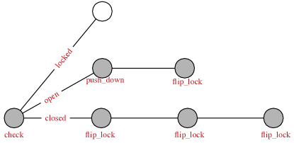
Figure 1: A plan tree

For a plan $p$, let $w(p)$ be the number of leaves of $T_{p}$ and $h(p)$ be the number of nodes along the longest path from the root to the leaves of $T_{p}$. $w(p)$ and $h(p)$ are called the width and height of $T_{p}$ respectively. Suppose $w$ and $h$ are two integers that such that $w(p)\leq w$ and $h(p)\leq h$.

Let us denote the leaves of $T_{p}$ by $x_{1},\ldots,x_{w(p)}$. We map each node $y$ of $T_{p}$ to a pair of integers $n_{y}$ = ($t_{y}$,$p_{y}$), where $t_{y}$, called the $t$-value of $y$, is the number of nodes along the path from the root to $y$ minus 1, and $p_{y}$, called the $p$-value of $y$, is defined in the following way:

• For each leaf $x_{i}$ of $T_{p}$, $p_{x_{i}}$ is an arbitrary integer between $0$ and $w$. Furthermore, there exists a leaf $x$ such that $p_{x}=0$, and there exist no $i\neq j$ such that $p_{x_{i}}=p_{x_{j}}$.

• For each interior node $y$ of $T_{p}$ with children $y_{1},\ldots,y_{r}$, $p_{y}=\min\{p_{y_{1}},\ldots,p_{y_{r}}\}$.

For instance, Figure 2 shows some possible mappings with $h=3$ and $w=3$ for the tree in Figure 1.

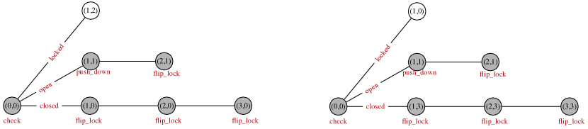
Figure 2: Possible mappings for the tree in Figure 1

It is easy to see that if $w(p)\leq w$ and $h(p)\leq h$ then such a mapping always exists. Furthermore, from the construction of $T_{\alpha}$, independently of how the leaves of $T_{\alpha}$ are numbered, we have the following properties.

1. For every node $y$, $t_{y}\leq h$ and $p_{y}\leq w$.

2. For a node $y$, all of its children have the same $t$-value. That is, if $y$ has $r$ children $y_{1},\ldots,y_{r}$ then $t_{y_{i}}=t_{y_{j}}$ for every $1\leq i,j\leq r$. Furthermore, the $p$-value of $y$ is the smallest one among the $p$-values of its children.

3. The root of $T_{\alpha}$ is always mapped to the pair $(0,0)$.

The numbering schema of a plan tree provides a method for generating a conditional plan on a two-dimensional coordinated system (or grid) where the x- and y-axis correspond to the height and width of the plan tree, and where $(0,0)$ is the initial state. Along a line of the same $y$-value is an action sequence and the execution of a sensing action creates branches on different lines, parallel to the $x$-axis. For example, the execution of the $check$ action in the initial state of the plan tree in Figure 2 creates three branches, to lines 0, 1, and 2. In the following, we use path to indicate the branch number and refer to a coordinate $(x,y)$ as a node.

Let us next describe the rules in program $\Pi_{h,w}(\mathcal{P})$. Intuitively, the program is similar to the program $\Pi^{a}(\mathcal{P},n)$ in that it implements the approximation $\Phi^{a}$ and extends it to deal with sensing actions. Since a conditional plan is two-dimensional, all predicates $holds$, $ph$, $possible$, $occ$, $de$, etc. need to extend with a third parameter. That is, $holds(L,T,P)$—encoding that $L$ holds at node $(T,P)$ (the time step $T$ and the line number $P$ on the two-dimensional grid)—is used instead of $holds(L,T)$. In addition, $\Pi_{h,w}(\mathcal{P})$ uses the following additional atoms and predicates.

• $path(0..w)$.

• $sense(a,g)$ if $g$ is a sensed literal which belongs to $\theta$ in a knowledge law of the form (31).

• $br(G,T,P,P_{1})$ is true if there exists a branch from $(T,P)$ to $(T+1,P_{1})$ labeled with $G$.

  For example, in Figure 2 (left), we have $br(open,0,0,1)$, $br(closed,0,0,0)$, and $br(locked,0,1,2)$.

• $used(T,P)$ is true if $(T,P)$ belongs to some extended branch of the plan tree. This allows us to know which paths are used in the construction of the plan and allows us to check if the plan satisfies the goal.

  In Figure 2 (left), we have $used(t,0)$ for $0\leq t\leq h$, and $used(t,1)$ and $used(t,2)$ for $1\leq t\leq h$.

The rules of $\Pi_{h,w}(\mathcal{P})$ are divided into two groups. The first group consists of rules from $\Pi^{a}(\mathcal{P},n)$ adapted to the two dimensional array for conditional planning. The second group consists of rules for dealing with sensing actions. We next describe the first group of rules in $\Pi_{h,w}(\mathcal{P})$:

$$holds(\Gamma,0,0) \leftarrow$$ (33)

$$possible(a,T,P) \leftarrow holds(\varphi,T,P)$$ (34)

$$holds(f,T+1,P) \leftarrow occ(a,T,P),holds(\varphi,T,P)$$ (35)

$$de(f,T+1,P) \leftarrow occ(a,T,P),holds(\varphi,T,P)$$ (36)

$$ph(f,T+1,P) \leftarrow occ(a,T,P),{not\>}h(\overline{\varphi},T,P),{not\>}de(\overline{f},T+1,P)\quad$$ (37)

$$ph(f,T,P) {\leftarrow} ph(\varphi,T,P)$$ (38)

$$holds(f,T,P) \leftarrow holds(\varphi,T,P)$$ (39)

$$ph(L,T+1,P) \leftarrow fluent(L),{not\>}holds(\neg L,T),{not\>}de(\neg L,T,P)$$ (40)

$$ph(\neg L,T+1,P) \leftarrow fluent(L),{not\>}holds(L,T),{not\>}de(L,T,P)$$ (41)

$$holds(L,T+1,P) \leftarrow fluent(L),{not\>}ph(\neg L,T,P)$$ (42)

$$holds(\neg L,T+1,P) \leftarrow fluent(L),{not\>}ph(L,T,P)$$ (43)

$$1\{occ(X,T,P):action(X)\}1 \leftarrow used(T,P),{not\>}goal(T,P)$$ (44)

$$\leftarrow occ(A,T,P),{not\>}possible(A,T,P)$$ (45)

In the above rules, $L$ is a fluent literal, $T$ is a time moment in the range $[0,h-1]$, and $P$ is in the range $[0,w]$. Rule (33) encodes the initial state. The rules (34)–(43) are used for computing the effects of the occurrence of a non-sensing action at the node $(T,P)$. The rules (44) and (45) are used for generating action occurrences, similarly to the rules for generating action occurrences in the previous sections. The difference is that the selection restricts the generation of action occurrences to nodes marked as ‘used’ (see below).

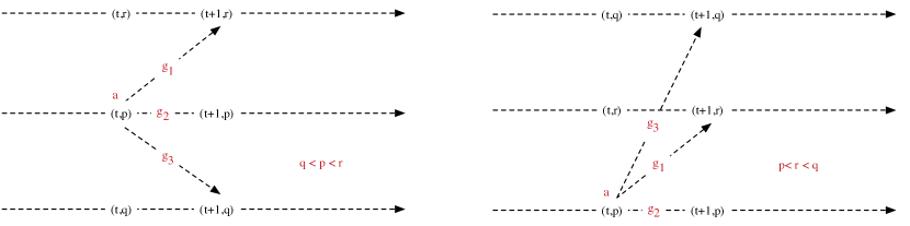
Figure 3: Sensing action $a$ that senses $\{g_{1},g_{2},g_{3}\}$ occurs at $(t,p)$ - disallowed (Left) vs. allowed (Right)

The key distinction between $\Pi_{h,w}(\mathcal{P})$ and $\Pi^{a}(\mathcal{P},n)$ lies in the rules for dealing with sensing actions. We next describe this set of rules.

• Rules for reasoning about the effect of sensing actions: For each knowledge law (31) in $D$, $\Pi_{h,w}(\mathcal{P})$ contains the following rules:

  $$1\{br(g,T,P,X){:}new\_br(P,X)\}1 \leftarrow occ(a,T,P),sense(a,g).$$ (48)

  $$\leftarrow occ(a,T,P),sense(a,g),$$

  $${not\>}br(g,T,P,P)$$

  $$\leftarrow occ(a,T,P),sense(a,g),$$

  $$holds(g,T,P)$$

  $$new\_br(P,P_{1}) \leftarrow P\leq P_{1}$$ (49)

  When a sensing action occurs, it creates one branch for each of its sensed literals. This is encoded in the rule (48). The constraint (48) makes sure that the current branch $P$ is continuing if a sensing action occurs at $(T,P)$. The rule (48) is a constraint that prevents a sensing action to occur if one of its sensed literals is already known. To simplify the selection of branches, rule (49) forces a new branch at least at the same level as the current branch. The intuition behinds these rules can be seen in Figure 3.

• Inertia rules for sensing actions: This group of rules encodes the fact that the execution of a sensing action does not change the world. However, there is a one-to-one correspondence between the set of sensed literals and the set of possible partial states.

  $$\leftarrow P_{1}<P_{2},P_{2}<P,br(G_{1},T,P_{1},P),$$ (51)

  $$br(G_{2},T,P_{2},P)$$

  $$\leftarrow P_{1}\leq P,G_{1}\neq G_{2},br(G_{1},T,P_{1},P),$$

  $$br(G_{2},T,P_{1},P)$$

  $$\leftarrow P_{1}<P,br(G,T,P_{1},P),used(T,P)$$ (52)

  $$used(T+1,P) \leftarrow P_{1}<P,br(G,T,P_{1},P)$$ (53)

  $$holds(G,T+1,P) \leftarrow P_{1}\leq P,br(G,T,P_{1},P)$$ (54)

  $$holds(L,T+1,P) \leftarrow P_{1}<P,br(G,T,P_{1},P),holds(L,T,P_{1})$$ (55)

  $$used(0,0) \leftarrow$$ (56)

  $$used(T+1,P) \leftarrow used(T,P)$$ (57)

  The first three rules, together with rule (49), make sure that branches are separate from each other. The next rule is used to mark a node as used if there is a branch in the plan that reaches that node. This allows us to know which paths on the grid are used in the construction of the plan and allows us to check if the plan satisfies the goal (see rule (58)). The two rules (54)–(55), along with rule (53), encode the possible partial state corresponding to the branch denoted by literal $G$ after a sensing action is performed at $(T,P_{1})$. They indicate that the partial state at $(T+1,P)$ should contain $G$ (Rule (54)) and literals that hold in $(T,P_{1})$ (Rule (55)). The last two rules mark nodes that have been used in the construction of the conditional plan.

• Goal representation: Checking for goal satisfaction needs to be done on all branches. This is encoded as follows.

  $$goal(T_{1},P) \leftarrow holds(\Delta,T_{1},P)$$ (58)

  $$goal(T_{1},P) \leftarrow holds(L,T_{1},P),holds(\neg L,T_{1},P)$$ (59)

  $$\leftarrow used(h+1,P),{not\>}goal(h+1,P)$$ (60)

  The first rule in this group says that the goal is satisfied at a node if all of its subgoals are satisfied at that node. The last rule guarantees that if a path $P$ is used in the construction of a plan then the goal must be satisfied at the end of this path, that is, at node $(h,P)$. The second rule provides an avenue to stop the generation of actions when an inconsistent state is encountered—by declaring the goal reached. As discussed by Tu et al. (2007), the properties of the encoding of consistent action theories prevent this method from generating plans leading to inconsistent states.

Remark 4

1. $\Pi_{h,w}(\mathcal{P})$ is slightly different from the program presented in the paper by Tu et al. (2007) in that $\Phi^{a}$ is slightly different from the semantics used in that paper. By setting $w=0$, this program is a conformant planner. The experiments conducted by Tu et al. (2007) show that $\Pi_{h,w}(\mathcal{P})$ performs reasonably well.

2. Extracting a conditional plan from an answer set $S$ of $\Pi_{h,w}(\mathcal{P})$ is not as simple as it is done in the previous sections because of the case-plan. For any pair of integers $i$ and $k$ such that $0\leq i\leq h,0\leq k\leq w$, we define $p^{k}_{i}(S)$ as follows:

   $$p^{k}_{i}(S)=\left\{\begin{array}[]{ll}\langle\rangle&\textnormal{if }i=h\textnormal{ or }occ(a,i,k)\not\in S\textnormal{ for all }a\\ \langle a;p^{k}_{i+1}(S)\rangle&\textnormal{if }occ(a,i,k)\in S\textnormal{ and }\\ &a\textnormal{ is a non-sensing action}\\ \langle a;{\bf cases}(\{g_{j}\rightarrow p_{i+1}^{k_{j}}(S)\}^{n}_{j=1})\rangle&\textnormal{if }occ(a,i,k)\in S,\\ &a\textnormal{ is a sensing action},\textnormal{and }\\ &br(g_{j},i,k,k_{j})\in S\textnormal{ for }1\leq j\leq n\end{array}\right.$$

   Intuitively, $p^{k}_{i}(S)$ is the conditional plan whose corresponding tree is rooted at node $(i,k)$ on the grid $h\times w$. Therefore, $p^{0}_{0}(S)$ is a solution to $\mathcal{P}$.

3. The semantics of $\mathcal{B}$ with knowledge laws does not prevent a sensing action to occur when some of its sensed literals is known. It is easy to see that in this case, the branching, enforced by rule (48), is unnecessary. Rule (48) disallows such redundant action occurrences. It is shown by Tu et al. (2007) that any solution of $\mathcal{P}=\langle D,\Gamma,\Delta\rangle$ can be reduced to an equivalent plan without redundant occurrences of sensing actions which can be found by $\Pi_{h,w}(\mathcal{P})$.

4. Because the execution of a sensing action creates multiple branches and some of them might be inconsistent (Eq. (32)), rule (59) prevents any action to occur at node $(T,P)$ when the partial state at $(T,P)$ is inconsistent. To mark that the path ends at this node, we say that the goal is achieved. Tu et al. (2007) showed that for a consistent planning problem, any solution generated by $\Pi_{h,w}(\mathcal{P})$ corresponds to a correct solution.

5. The comparison between ASP-based systems, like CPasp and $\Pi_{h,w}(\mathcal{P})$, and conformant planning or conditional planning systems, such as CMBP Cimatti and Roveri (2000), dlv^K Eiter et al. (2003b), C-Plan Castellini et al. (2003), CFF Brafman and Hoffmann (2004), KACMBP Cimatti et al. (2004), $t_{0}$ Palacios and Geffner (2007), and POND Bryce et al. (2006), has been presented in the papers by Tu et al. (2007) and 2011. The comparison shows that ASP-based planning systems perform much better than other systems in domains with static causal laws.

6. $\Pi_{h,w}(\mathcal{P})$, similar to CPasp, makes a single call to the ASP solver to compute a conditional plan. This is possible because of it uses an approximation semantics that reduces the complexity of conditional planning, for polynomially-bounded plan, to NP-complete. Otherwise, this would not be possible because conditional planning for polynomially-bounded length plan is PSPACE-complete Turner (2002). Naturally, as with CPasp, this also implies that $\Pi_{h,w}(\mathcal{P})$ is incomplete.

5.3 Context: Conditional Planning

As we mentioned earlier, the need for plans with conditionals and/or loops has been identified very earlier on by Warren (1976), who developed Warplan-C, a Prolog program that can generate conditional plans and programs given the problem specification. Warplan-C has only 66 clauses and is conjectured to be complete. The system was developed at the same time as other non-linear planning systems, such as Noah by Sacerdoti (1974). These earlier systems do not deal with sensing actions. Other systems that generate plans with if-then statements and can prepare for contingencies are Cassandra Pryor and Collins (1996) and CNLP Peot and Smith (1992). These two systems extend partial order planning algorithms for computing conditional plans.

XII Golden et al. (1996) and PUCCINI Golden (1998) are two systems that employ partial order planning to generate conditional plans for problems with incomplete information and can deal with sensing actions. SGP Weld et al. (1998) and POND Bryce et al. (2006) are conditional planners that work with sensing actions. These systems extend the planning graph algorithm Blum and Furst (1997) to deal with sensing actions. The main difference between SGP and POND is that the former searches solutions within the planning graph, whereas the latter uses it as a means of computing the heuristic function.

CoPlaS, developed by Lobo (1998), is a regression Prolog-based planner that uses a high-level action description language, similar to the language $\mathcal{B}_{K}$ described in this section, to represent and reason about effects of actions, including sensing actions. Van Nieuwenborgh et al. (2007) introduced $\mathcal{K}_{c}$, an extension of language $\mathcal{K}$, to deal with sensing actions and compute conditional plans as defined in this section using dlv^K. Thielscher (2000) presented FLUX, a constraint logic programming based planner, which is capable of generating and verifying conditional plans. QBFPlan is another conditional planner, based on a QBF theorem prover, is described in the paper by Rintanen (1999). This system, however, does not consider sensing actions.

Research in developing conditional planners, however, has not attracted as much attention compared to other types of planning domains in recent years. Rather, the focus has been on synthesizing controllers or reactive modules which exhibit specific behaviors in different environments Aminof et al. (2020); Camacho et al. (2019, 2018); Treszkai and Belle (2020). This is similar to the effort of generating programs satisfying a specification as discussed earlier (e.g., the work by Warren (1976)) or attempts to compute policies (see, e.g., the book by Bellman (1957)) for Markov Decision Processes (MDP) or Partially Observable Markov Decision Processes (POMDP). To the best of our knowledge, little attention has been paid to this research direction within the ASP community. We present this as a challenge to ASP in the last section of the paper.

6 Planning with Preferences

The previous sections analyze answer set planning with the focus on solving different classes of planning problems, such as planning with complete information, incomplete information, and sensing actions. In this section, we present another extension of the planning problem, by illustrating the use of answer set planning in planning with preferences.

The problem of planning with preferences arises in situations where the user not only wants a plan to achieve a goal, but has specific preferences or biases about the plan. This situation is common when the space of possible plans for a goal is dense, i.e., finding “a” plan is not difficult, but many of the plans may have features which are undesirable to the user. This type of situations is very common in practical planning problems.

Example 7

Traveling from one place to another is a frequently considered problem (e.g., a traveler, a transportation vehicle, an autonomous vehicle). A planning problem in the travel domain can be represented by the following elements:

• a set of fluents of the form $at(\ell)$, where $\ell$ denotes a location, such as home, school, neighbor, airport, etc.;

• an initial location $\ell_{i}$;

• a destination location $\ell_{f}$; and

• a set of actions of the form $method(\ell_{1},\ell_{2})$ where $\ell_{1}$ and $\ell_{2}$ are two distinct locations and $method$ is one of the available transportation methods, such as drive, walk, ride_train, bus, taxi, fly, bike, etc. The problem may include conditions that restrict the applicability of actions in certain situations. For example, one can ride a taxi only if the taxi has been called, which can be done only if one has some money; one can fly from one place to another if one has a ticket; etc.

Problems in this domain are often rich in solutions because of the large number of actions which can be used in the construction of a plan. For this reason, a user looking for a solution to a problem often considers some additional features, or personal preferences, in selecting a plan. For example, the user might be biased in terms of the distance to travel using a transportation method, the overall cost, the time to destination, the comfort of a vehicle, etc. However, a user would accept a plan that does not satisfy her preferences if she has no other choice. $\Diamond$

Preferences can come in different shapes and forms. The most common types of preferences are:

• Preferences about a state: the user prefers to be in a state $s$ that satisfies a property $\phi$ rather than a state $s^{\prime}$ that does not satisfy it, in case both lead to the satisfaction of the goal; for example, being in a 5-star hotel is preferable to being in a 1-star hotel, if the distance to the conference site is the same;

• Preferences about an action: the user prefers to perform (or avoid) an action $a$, whenever it is feasible and it allows the goal to be achieved; for example, one might prefer to walk to destination whenever possible;

• Preferences about a trajectory: the user prefers a trajectory that satisfies a certain property $\psi$ over those that do not satisfy this property; for example, one might prefer plans that do not involve traveling through Los Angeles during peak traffic hours;

• Multi-dimensional preferences: the user has a set of preferences, with an ordering among them. A plan satisfying a more favorable preference is given priority over those that satisfy less favorable preferences; for example, plans that minimize time to destination might be preferable to plans minimizing cost.

Son and Pontelli (2006) propose a general method for integrating diverse classes of preferences into answer set planning. Their approach is articulated in two components:

• Development of a preference specification language: this language supports the specification of different types of preferences; its semantics should enable the definition of a partial order among possible solutions of the planning problem.

• Implementation: the implementation proposed by Son and Pontelli (2006) maps preference formulae to mathematical formulae, representing the weight of each formula, and makes use of the $\mathtt{maximize}$ statement in answer set programming to optimize the solution to the planning problem. The original paper defines rules for computing the weights of preference formulae in ASP.

We next introduce the preference specification language proposed by Son and Pontelli (2006).

6.1 A Preference Specification Language

The proposed preference specification language addresses the description of three classes of preferences: basic desires, atomic preferences, and general preferences.

For a planning problem $\mathcal{P}=\langle D,\Gamma,\Delta\rangle$, a basic desire can be in of the following possible forms:

• a state formula, which is a fluent formula $\varphi$ or a formula of the form $occ(a)$ for some action $a$, or

• a goal preference, of the form $\textbf{goal}(\varphi)$, where $\varphi$ is a fluent formula.

Basic desire formula.

A basic desire formula is a formula built over basic desires, the traditional propositional operators ($\wedge$, $\vee$, and $\neg$), and the modalities next, always, eventually, and until. The BNF for the basic desire formulae is

$$\psi\stackrel{{\scriptstyle def}}{{=}}\varphi\mid\psi_{1}\wedge\psi_{2}\mid\psi_{1}\vee\psi_{2}\mid\neg\psi_{1}\mid\hbox{\bf next}(\psi_{1})\mid\hbox{\bf until}(\psi_{1},\psi_{2})\mid\hbox{\bf always}(\psi_{1})\mid\hbox{\bf eventually}(\psi),$$

where $\varphi$ represents a state formula or a goal preference and $\psi$, $\psi_{1}$, or $\psi_{2}$ are basic desire formulae.

Intuitively, a basic desire formula specifies a property that a user would like to see satisfied by the provided plan. For example, to express the fact that a user would like to take the taxi or the bus to go to school, we can write:

$$\hbox{\bf eventually}(\>occ(bus(home,school))\vee occ(taxi(home,school))\>).$$

If the user’s desire is not to call a taxi, we can write

$$\hbox{\bf always}(\>\neg occ(call\_taxi(home))\>).$$

If the user’s desire is not to see any taxi around his home, we can use the basic desire formula

$$\hbox{\bf always}(\>\neg available\_taxi(home)\>).$$

Note that these encodings have different consequences—the last formula prevents taxis to be present, independently from whether the taxi has been called.

The following are several basic desire formulae that are often of interest to users.

• Strong Desire: For two formulae $\varphi_{1}$ and $\varphi_{2}$, $\varphi_{1}<\varphi_{2}$ denotes $\varphi_{1}\wedge\neg\varphi_{2}$.

• Weak Desire: For two formulae $\varphi_{1}$ and $\varphi_{2}$, $\>\>\varphi_{1}<^{w}\varphi_{2}$ denotes $\varphi_{1}\vee\neg\varphi_{2}$.

• Enabled Desire: For two actions $a_{1}$ and $a_{2}$, $a_{1}<^{e}a_{2}$ stands for
  $(executable(a_{1})\wedge executable(a_{2}))\Rightarrow(occ(a_{1})<occ(a_{2}))$ where
  $executable(a)=\bigwedge_{l\in\varphi}l$ if $\hbox{\bf executable}(a,\varphi)\in D$.

• Action Class Desire: For actions with the same set of parameters and effects such as drive or walk, we write $drive<^{e}walk$ to denote the desire
  $\bigvee_{l_{1},l_{2}\in S,\>l_{1}\neq l_{2}}(drive(l_{1},l_{2})<^{e}walk(l_{1},l_{2}))$ where $S$ is a set of pre-defined locations. Intuitively, this preference states that we prefer to drive rather than to walk between locations belonging to the set $S$. For example, if $S=\{home,school\}$ then this preference says that we prefer to drive from home to school and vice versa.

Atomic preference.

Basic desire formulae are expressive enough to describe a significant portion of preferences that frequently occur in real-world domains. It is also often the case that the user may provide a variety of desires, and some desires are stronger than others; knowledge of such biases about desires becomes important when it is not possible to concurrently satisfy all the provided desires. In this situation, an ordering among the desires is introduced. An atomic preference formula is a formula of the form

$$\varphi_{1}\lhd\varphi_{2}\lhd\cdots\lhd\varphi_{n}$$

where $\varphi_{1},\dots,\varphi_{n}$ are basic desire formulae. The atomic preference formula states that trajectories that satisfy $\varphi_{1}$ are preferable to those that satisfy $\varphi_{2}$, etc.

Let us consider again the travel domain. Besides time and cost, users often have their preferences based on the level of comfort and/or safety of the available transportation methods. These preferences can be represented by the formulae

$$\mathit{cost}=\hbox{\bf always}(\mathit{walk}<^{e}\mathit{bus}<^{e}\mathit{drive}<^{e}\mathit{flight})$$

and

$$\mathit{time}=\hbox{\bf always}(\mathit{flight}<^{e}\mathit{drive}<^{e}\mathit{bus}<^{e}\mathit{walk})$$

and

$$\mathit{comfort}=\hbox{\bf always}(\mathit{flight}<^{e}(drive\vee bus)<^{e}walk)$$

and

$$\mathit{safety}=\hbox{\bf always}(walk<^{e}\mathit{flight}<^{e}(drive\vee bus)).$$

These four desires can be combined to produce the following two atomic preferences

$$\Psi^{t}_{1}=\mathit{comfort}\lhd\mathit{safety}\>\>\>\textnormal{ and }\>\>\>\Psi^{t}_{2}=cost\lhd time.$$

Intuitively, $\Psi^{t}_{1}$ is a comparison between level of comfort and safety, while $\Psi^{t}_{2}$ is a comparison between affordability and duration.

General preference formulae.

Suppose that a user would like to travel as comfortably and as cheaply as possible. Such a preference can be viewed as a multi-dimensional preference, which cannot be easily captured using atomic preferences or basic desires. General preference formulae support the representation of such multi-dimensional preferences.

Formally, a general preference formula is a formula satisfying one of the following conditions:

• An atomic preference $\Psi$ is a general preference;

• If $\Psi_{1},\Psi_{2}$ are general preferences, then $\Psi_{1}\&\Psi_{2}$, $\Psi_{1}\mid\Psi_{2}$, and $!\>\Psi_{1}$ are general preferences;

• If $\Psi_{1},\Psi_{2},\dots,\Psi_{k}$ is a collection of general preferences, then $\Psi_{1}\lhd\Psi_{2}\lhd\cdots\lhd\Psi_{k}$ is a general preference.

In the above definition, the operators $\&,\mid,!$ are used to express different ways to combine preferences. For example, the preference $\Psi^{t}_{1}\&\Psi^{t}_{2}$ indicates that the user prefers trajectories that are most preferred according to both $\Psi^{t}_{1}$ and $\Psi^{t}_{2}$; $\Psi^{t}_{1}\mid\Psi^{t}_{2}$ states that, among trajectories with the same cost, the user prefers trajectories that are most comfortable or vice versa. A detailed discussion of general preferences can be found in the paper by Son and Pontelli (2006).

Semantics.

In order to define the semantics of the preference language, we need to start from describing whether a trajectory $\alpha=s_{0}a_{0}\ldots a_{n-1}s_{n}$ satisfies a basic desire formula. We write $\alpha\models\varphi$ to denote that $\alpha$ satisfies a basic desire $\varphi$. The definition of $\models$ is straightforward, and we report here only some of the cases (the complete definition can be found in the paper by Son and Pontelli (2006)), where $\alpha[i]=s_{i}a_{i}\ldots a_{n-1}s_{n}$.

• $\alpha\models occ(a)$ if $a_{0}=a$;

• $\alpha\models\ell$ if $s_{0}\models\ell$ and $\ell$ is a fluent;

• $\alpha\models\hbox{\bf always}(\varphi)$ if for all $0\leq i<n$ we have $\alpha[i]\models\varphi$;

• $\alpha\models\hbox{\bf next}(\varphi)$ if $\alpha[1]\models\varphi$.

The satisfaction of desires is used to define two relations between trajectories, one expressing preference between trajectories and one capturing the fact that two trajectories are indistinguishable, denoted by $\prec_{\Psi}$ and $\approx_{\Psi}$, respectively, where $\Psi$ is a preference formula. For two trajectories $\alpha$ and $\beta$,

1. if $\Psi$ is a basic desire then $\alpha\prec_{\Psi}\beta$ ($\alpha$ is more preferred than $\beta$ with respect to $\Psi$) if $\alpha\models\Psi$ and $\beta\not\models\Psi$; $\alpha\approx_{\Psi}\beta$ denotes that $\alpha\models\Psi$ iff $\beta\models\Psi$.

2. if $\Psi$ is an atomic preference $\varphi_{1}\lhd\varphi_{2}\lhd\cdots\lhd\varphi_{n}$ then $\alpha\prec_{\Psi}\beta$ if $\exists(1\leq i\leq n)$ such that

   1. $\forall(1\leq j<i)$ we have that $\alpha\approx_{\varphi_{j}}\beta$, and

   2. $\alpha\prec_{\varphi_{i}}\beta$.

   $\alpha\approx_{\Psi}\beta$ denotes that $\alpha\approx_{\varphi_{j}}\Psi$ for every $j=1,\ldots,n$.

3. if $\Psi$ is a general preference and has the form $\Psi=\Psi_{1}\lhd\cdots\lhd\Psi_{k}$ then $\alpha\prec_{\Psi}\beta$ is defined similar to the second case. Otherwise, $\alpha\prec_{\Psi}\beta$

   1. if $\Psi=\Psi_{1}\&\Psi_{2}$ and $\alpha\prec_{\Psi_{1}}\beta$ and $\alpha\prec_{\Psi_{2}}\beta$

   2. if $\Psi=\Psi_{1}\mid\Psi_{2}$ and (i) $\alpha\prec_{\Psi_{1}}\beta$ and $\alpha\approx_{\Psi_{2}}\beta$; or (ii) $\alpha\prec_{\Psi_{2}}\beta$ and $\alpha\approx_{\Psi_{1}}\beta$; or (iii) $\alpha\prec_{\Psi_{1}}\beta$ and $\alpha\prec_{\Psi_{2}}\beta$.

   3. if $\Psi=\>!\Psi_{1}$ and $\beta\prec_{\Psi_{1}}\alpha$.

   In all cases, $\alpha\approx_{\Psi}\beta$ iff $\alpha\approx_{\Psi^{\prime}}\beta$ where $\Psi^{\prime}$ is a component of $\Psi$.

The following proposition holds Son and Pontelli (2006).

Proposition 1

$\prec_{\Psi}$ is a partial order and $\approx_{\Psi}$ is an equivalent relation.

The above proposition shows that maximal elements with respect to $\prec_{\Psi}$ exist, i.e., most preferred trajectories exist.

6.2 Implementation: Computing Preferred Plans

Given a planning problem $\mathcal{P}$ and a preference formula $\Psi$, a preferred trajectory can be computed using the following steps:

1. Use one of the programs, denoted by $\mathit{Plan}(\mathcal{P},n)$, introduced in Sections 3–4 to compute a potential solution $\alpha$ for $\mathcal{P}$ ;

2. Associate to $\alpha$ a number, which represents the degree of satisfaction of $\alpha$ with respect to $\Psi$; and

3. Use the $\#maximize$ statement of clingo to compute a most preferred trajectory.

This process requires an appropriate encoding of $\Psi$. This is usually achieved by converting $\Psi$ to a canonical form, which provides a convenient way to translate $\Psi$ into a set of facts with predefined predicates. For example, a basic desire formula can be encoded using the predicates and, or, $\neg$, occ, next, until, eventually, always, and final (stands for goal, to avoid confusion with the goal predicate defined in the previous sections). This translation can be done using a script (e.g., Son and Pontelli (2006) presented a Prolog program for such translation).

An atomic preference can be represented using an ordered set, consisting of a declaration $atomic(id)$, indicating that $id$ is an atomic preference, and a set of atoms of the form $member(id,\mathit{formula},order)$, where $id$, formula, and order represent the atomic preference identifier, the formula, and the order of the formula in $id$, respectively. Finally, a general preference can be encoded using the predicates $\&$, $\mid$, and $!$, and the basic representations of basic desires and atomic preferences. In the following, we use $\Pi(\Psi)$ to denote the set of facts encoding $\Psi$.

Since the first task in computing a most preferred trajectory is checking whether or not a trajectory satisfies a basic desire, we need to add to $\mathit{Plan}(\mathcal{P},n)$ rules for this purpose. This task can be achieved by a set of domain-independent rules $\Pi_{\mathit{pref}}$ defining the predicate $holds(sat(\varphi),t)$, which states that the basic desire formula $\varphi$ is satisfied by the trajectory $s_{t}a_{t}\ldots a_{n-1}s_{n}$. $\Pi_{\mathit{pref}}$ contains the following groups of rules:

• Rules for checking the satisfaction of a propositional formula at a time step: such as

  $$\begin{array}[]{lcl}holds(sat(F),T)&\leftarrow&fluent(F),holds(F,T)\\ holds(sat(and(F,G)),T)&\leftarrow&holds(sat(F),T),holds(sat(G),T)\end{array}$$

• Rules for checking the satisfaction of a temporal formula at a time step: such as

  $$holds(sat(\hbox{\bf next}(F)),T)\leftarrow holds(sat(F),T+1)$$

• Rules for checking the occurrence of an action:

  $$holds(sat(occ(A)),T)\leftarrow occ(A,T)$$

• Rules for checking the satisfaction of a goal formula:

  $$holds(sat(final(F)),0)\leftarrow holds(sat(F),n)$$

The following proposition holds.

Proposition 2

An answer set $S$ of $\mathit{Plan}(\mathcal{P},n)\cup\Pi(\varphi)\cup\Pi_{\mathit{pref}}$ contains $holds(sat(\varphi),0)$ if and only if the trajectory corresponds to $S$ satisfies $\varphi$.

The above proposition shows that $\mathit{Plan}(\mathcal{P},n)\cup\Pi(\varphi)\cup\Pi_{\mathit{pref}}$ can be used to compute a most preferred trajectory with respect to a basic desire formula. To do so, we only need to tell clingo that an answer set containing $holds(sat(\varphi),0)$ is preferred.

To compute a most preferred plan with respect to a general preference or an atomic formula, Son and Pontelli (2006) proposed a set of rules that assigns a number to a formula and then use the $\#maximize$ statement of clingo to select a most preferred trajectory. The proposed rules were developed at the time the answer set solvers did provide only limited capability to work with numbers. For this reason, we omit the detail about these rules here. Features provided in more recent versions of answer set solvers, such as multiple optimization statements and weighted tuples, are likely to enable a simpler and more efficient implementation. For example, we could translate an atomic preference

$$\varphi_{1}\lhd\varphi_{2}\ldots\lhd\varphi_{n}$$

to a statement

$$\#maximize\{1@n:holds(sat(\varphi_{1}),0);\ldots;n@1:holds(sat(\varphi_{n}),0)\}$$

as a part of $\Pi(\Psi)$.

Remark 5

1. The encoding of $\Pi(\Psi)$ presented in this paper does not employ any advanced features of answer set programming, which were introduced to simplify the encoding of preferences such as the framework for preferences specification asprin, introduced by Brewka et al. (2015a) and 2015b. Analogously, a more elegant encoding of preference formulae can be achieved using other extensions of answer set programming focused on rankings of answer sets, such as logic programming with ordered disjunctions Brewka (2002). This encoding, however, cannot be used with clingo or dlv because none of these solvers supports ordered disjunctions.

2. The discussion in this section focuses on expressing preferences over trajectories, i.e., sequences of actions and states. It can be extended to conditional plans and used with the planner in Section 5. This extension can, for example, define preferences over branches in a conditional plan.

6.3 Context: Planning with Preferences

Planning with preferences has attracted a lot of attention by the planning community. An excellent survey of several systems developed before 2008 and their strengths and weaknesses can be found in the paper by Baier and McIlraith (2008). Preferences have also been included in extensions of PDDL, such as PDDL3 Gerevini and Long (2005). The majority of systems described in the survey employ PDDL3 where preferences are, ultimately, described by a numeric value. As such, most of the planning with preferences systems in the literature can be characterized as cost optimal, where the cost of actions plays a key role in deciding the preference of a solution. Hierarchical task planning is also frequently used in these systems. Representative systems in this direction are HPlan-P Sohrabi et al. (2009), LPRPG-P Coles and Coles (2011), and PGPlanner Das et al. (2019). ChoPlan, developed by Bidoux et al. (2019), is a system which encodes a PDDL3 planning problem as a multi-attribute utility theory and a heuristic based on Choquet integrals to derive solutions.

satplan(P), developed by Giunchiglia and Maratea (2007), shows that SAT-based planning is also competitive with other planning paradigms. Giunchiglia and Maratea (2011) present a survey of SAT-based planning with preferences. In recent years, SMT-based planning has become more popular than SAT-based planning, thanks to the expressiveness of SMT compared to SAT and the availability of efficient SMT solvers. SMT-based planning, which can work with numeric variables, provides an excellent way to deal with preferences Scala et al. (2016). It is worth observing that ASP-based planning with action costs has been considered earlier by Eiter et al. (2003a) and more recently by Khandelwal et al. (2014).

7 Planning and Diagnosis

While planning and diagnosis are often considered two separate and independent tasks, some researchers have suggested that ties exist between them, to the point that it is possible to reduce diagnostic reasoning to planning. In this section, we present this view, and specifically focus on the approach from Baral and Gelfond (2000) and Balduccini and Gelfond (2003), under which planning tasks and diagnostic tasks share (a) the same domain representation and (b) the same core reasoning algorithms.

In this section, the term diagnosis describes a type of reasoning task in which an agent identifies and interprets discrepancies between the domain’s expected behavior and the domain’s actual/observed behavior. Consider the following example.

Example 8 (From the paper by Balduccini and Gelfond (2003))

Consider the analog circuit $\cal{AC}$ from Figure 4.

Figure 4: Analog circuit $\cal{AC}$

We assume that switches $sw_{1}$ and $sw_{2}$ are mechanical components that cannot be damaged. Relay r is a magnetic coil. If not damaged, it is activated when $sw_{1}$ is closed, causing $sw_{2}$ to close. Undamaged bulb $b$ emits light if $sw_{2}$ is closed. For simplicity of presentation we consider an agent capable of performing only one action, $close(sw_{1})$. The environment can be represented by two damaging exogenous actions: $brk$, which causes $b$ to become faulty, and $srg$, which damages $r$ and also $b$ assuming that $b$ is not protected. Suppose that the agent operating this device is given a goal of lighting the bulb. He realizes that this can be achieved by closing the first switch, performs the operation, and discovers that the bulb is not lit. The domain’s behavior does not match the agent’s expectations. The agent needs to determine the reason for this state of affairs and ways to correct the problem. $\Diamond$

In the following, we focus on non-intrusive and observable domains, in which the agent’s environment does not normally interfere with his work and the agent normally observes all of the domain occurrences of exogenous actions. The agent is, however, aware that these assumptions can be contradicted by observations. The agent is ready to observe and to take into account occasional occurrences of exogenous actions that alter the behavior of the environment. Moreover, discrepancies between expectations and observations may force the agent to conclude that additional exogenous actions have occurred, but remained unobserved.

To model the domain, let us introduce a finite set of components C, disjoint from A and F previously introduced. Let us also assume the existence of a set F₀ $\subseteq$ F of observable fluents (i.e., fluents that can be directly observed by the agent), such that $ab(c)\in$ F₀ for every component of C. Fluent $ab(c)$ intuitively indicates that the $c$ is “faulty.” Let us point out that the use of the relation $ab$ in diagnosis dated back to the work by Reiter (1987). The set A is further partitioned into two disjoint sets: A_s, corresponding to agent actions, and A_e consisting of exogenous actions. Additionally, exogenous and agent actions are allowed to occur concurrently. With respect to the formalization methodology introduced in Section 2.2, this is achieved by (1) introducing the notion of compound action, i.e., a set of agent and exogenous actions, (2) redefining $\Phi(a,s)$ so that $a$ is a compound action, and (3) extending the notion of trajectory to be a sequence $s_{0}a_{0}\ldots a_{k-1}s_{k}$ of states and compound actions.

A core principle of this approach is that the discrepancies between agent’s expectations and observations are explained in terms of occurrences of unobserved exogenous actions. The observed behavior of the domain is represented by a particular trajectory, referred to as the actual trajectory.

A diagnostic domain is a pair $\langle D,W\rangle$ where $D$ is a domain and $W$ is the domain’s actual trajectory.

Information about the behavior of the domain up to a certain step $n$ is captured by the recorded history $H_{n}$, i.e. a set of observations of the form:

1. $obs(l,t)$ – meaning that fluent literal $l$ was observed to be true at step $t$;

2. $hpd(a,t)$ – stating that action $a\in$ A was observed to happen at time $t$.

The link between diagnostic domain and recorded history is established by the following:

Consider a diagnostic domain $\langle D,W\rangle$ with $W=s^{w}_{0}a^{w}_{0}\ldots a^{w}_{n-1}s^{w}_{n}$, and let $H_{n}$ be a recorded history up to step $n$.

1. A trajectory $s_{0}a_{0}\ldots a_{n-1}s_{n}$ is a model of $H_{n}$ if for any $0\leq t\leq n$

   1. $a_{t}=\{a:hpd(a,t)\in H_{n}\}$;

   2. if $obs(l,t)\in H_{n}$ then $l\in s_{t}$.

2. $H_{n}$ is consistent if it has a model.

3. $H_{n}$ is sound if, for any $l$, $a$, and $t$, if $obs(l,t),hpd(a,t)\in H_{n}$ then $l\in s^{w}_{t}$ and $a\in a^{w}_{t}$.

4. A fluent literal $l$ holds in a model $M$ of $H_{n}$ at time $t\leq n$ ($M\models holds(l,t)$) if $l\in s_{t}$; $H_{n}$ entails $h(l,t)$($H_{n}\models holds(l,t)$) if, for every model $M$ of $H_{n}$, $M\models holds(l,t)$.

Note also that a recorded history may be consistent, but not sound – which is the case if the recorded history is incompatible with the actual trajectory.

Example 8 can thus be formalized as:

$$\begin{array}[]{l}\mbox{\% Fluents:}\\ fluent(active(r))\leftarrow\hskip 36.135ptfluent(on(b))\leftarrow\hskip 36.135ptfluent(prot(b))\leftarrow\\ fluent(closed(sw_{1}))\leftarrow\hskip 23.84923ptfluent(closed(sw_{2}))\leftarrow\\ fluent(ab(r))\leftarrow\hskip 52.03448ptfluent(ab(b))\leftarrow\\ \mbox{\% Agent Actions:}\\ a\_act(close(sw_{1}))\leftarrow\\ \mbox{\%Exogenous Actions}\\ x\_act(brk)\leftarrow\hskip 65.04256ptx\_act(srg)\leftarrow\end{array}$$

Note the use of relations $a\_act$ and $x\_act$ to distinguish agent actions and exogenous actions. The laws describing the normal and abnormal/malfunctioning behavior of the domain are:

$$D_{\mathcal{AC}}=\left\{\begin{array}[]{lll}\mbox{\% normal }&&\mbox{\% abnormal}\\ \hbox{\bf causes}(close(sw_{1}),closed(sw_{1}),\emptyset)&&\hbox{\bf causes}(brk,ab(b),\emptyset)\\ \hbox{\bf caused}(\{closed(sw_{1}),\neg ab(r)\},active(r))&&\hbox{\bf causes}(srg,ab(r),\emptyset)\\ \hbox{\bf caused}(\{active(r)\},closed(sw_{2}))&&\hbox{\bf causes}(srg,ab(b),\{\neg prot(b)\})\\ \hbox{\bf caused}(\{closed(sw_{2}),\neg ab(b)\},on(b))&&\hbox{\bf caused}(\{ab(b)\},\neg on(b))\\ \hbox{\bf caused}(\{\neg closed(sw_{2})\},\neg on(b))&&\hbox{\bf caused}(\{ab(r)\},\neg active(r))\\ \hbox{\bf executable}(close(sw_{1}),\{\neg closed(sw_{1})\})\end{array}\right.$$

Now consider a recorded history:

$$H_{1}=\left\{\begin{array}[]{l}hpd(close(sw_{1}),0)\\ obs(\neg closed(sw_{1}),0)\\ obs(\neg closed(sw_{2}),0)\\ obs(\neg ab(b),0)\\ obs(\neg ab(r),0)\\ obs(prot(b),0)\end{array}\right.$$

One can check that $s_{0}\ close(sw_{1})\ s_{1}$ is the only model of $H_{1}$, where $s_{0}$ is the state depicted in Figure 4. Additionally, $H_{1}\models holds(on(b),1)$.

Next, we formalize the key notions of diagnosis. Let $\delta=\langle D,W\rangle$ be a diagnostic domain. A configuration is a pair

$${\cal S}=\langle H_{n},O^{m}_{n}\rangle$$ (61)

where $H_{n}$ is the recorded history up to step $n$ and $O^{m}_{n}$ is a set of observations between steps $n$ and $m\geq n$. Leveraging this notion, we can now define a symptom as a configuration $\langle H_{n},O^{m}_{n}\rangle$ such that $H_{n}$ is consistent and $H_{n}\cup O^{m}_{n}$ is not.

Once a symptom has been identified, the next step of the diagnostic process aims at finding its possible reasons. Specifically, a diagnostic explanation $E$ of symptom ${\cal S}=\langle H_{n},O^{m}_{n}\rangle$ is defined as a set

$$E\subseteq\{hpd(a_{i},t):0\leq t<n\mbox{ and }a_{i}\in\mbox{\bf A}_{e}\},$$ (62)

such that $H_{n}\cup O^{m}_{n}\cup E$ is consistent.

7.1 Diagnostic Reasoning as Answer Set Planning

As we said earlier, answer set planning can be used to determine whether a diagnosis is needed and for computing diagnostic explanations. Next, we introduce an ASP-based program for these purposes. Consider a domain $D$ whose behavior up to step $n$ is described by recorded history $H_{n}$. Reasoning about $D$ and $H_{n}$ can be accomplished by a translation to a logic program $\Pi(D,H_{n})$ that follows the approach outlined in Section 3. Focusing for simplicity on the direct encoding, $\Pi(D,H_{n})$ consists of:

• the domain dependent rules from Section 3.1.1;

• the rules related to inertia and consistency of states (11)-(13);

• domain independent rule establishing the relationship between observations and the basic relations of $\Pi$:

  $$occ(A,T)\leftarrow hpd(A,T)$$ (63)

  $$holds(L,0)\leftarrow obs(L,0)$$ (64)

• the reality check axiom, i.e. a rule ensuring that in any answer set the agent’s expectations match the available observations (variable $L$ ranges over fluent literals):

  $$\leftarrow obs(L,T),{not\>}holds(L,T)$$ (65)

The following theorem establishes an important relationship between models of a recorded history and answer sets of the corresponding logic program.

Theorem 2

If the initial situation of $H_{n}$ is complete, i.e. for any fluent $f$, $H_{n}$ contains $obs(f,0)$ or $obs(\neg f,0)$, then $M$ is a model of $H_{n}$ iff $M$ is defined by some answer set of $\Pi(D,H_{n})$.

The proof of the theorem is in two steps. First, one shows that the theorem holds for $n=1$, i.e., that for a history $H_{1}$ there is a one-to-one correspondence between the transitions of the form $s_{0}a_{0}s_{1}$ and the answer sets of $\Pi(D,H_{1})$. Then, induction is leveraged to extend the correspondence to histories of arbitrary length. The complete proof can be found in the paper by Balduccini and Gelfond (2003).

Next, we focus on identifying the need for diagnosis. Given a domain $D$ and ${\cal S}=\langle H_{n},O^{m}_{n}\rangle$, we introduce:

$$\mathit{TEST}({\cal S})=\Pi(D,H_{n})\cup O^{m}_{n}.$$ (66)

The following corollary forms the basis of this approach to diagnosis.

Corollary 1

Let ${\cal S}=\langle H_{n},O^{m}_{n}\rangle$ where $H_{n}$ is consistent. A configuration ${\cal S}$ is a symptom iff $\mathit{TEST}({\cal S})$ has no answer set.

Once a symptom has been identified, diagnostic explanations can be found by means of the answer sets of the diagnostic program

$$\Pi_{d}({\cal S})=\mathit{TEST}({\cal S})\cup\{\ \ \ 1\{occ(A,T):x\_act(A)\}1\leftarrow time(T),T<n.\ \ \ \}$$ (67)

Specifically, every answer set $X$ of $\Pi_{d}({\cal S})$ encodes a diagnostic explanation

$$E=\{hpd(a,t)\,\,|\,\,occ(a,t)\in X\land a\in\mbox{{\bf A}${}_{e}$}\}.$$

Note that the choice rule shown in (67) is simply a restriction of (10) to exogenous actions. As a result, $\Pi_{d}({\cal S})$ can be viewed as a variant of the translation $\Pi(\mathcal{P},n)$ of a planning problem, where planning occurs over the past $0..n\!-\!1$ time steps and over exogenous actions only, and the goal states are described by the observations from ${\cal S}$.

Example 9

Consider the domain from Example 8. According to $H_{1}$ initially switches $sw_{1}$ and $sw_{2}$ are open, all circuit components are ok, $sw_{1}$ is closed by the agent, and b is protected. The expectation is that $b$ will be on at 1. Suppose that, instead, the agent observes that at time 1 bulb b is off, i.e. $O_{1}=\{obs(\neg on(b),1)\}$. $\mathit{TEST}({\cal S}_{0})$, where ${\cal S}_{0}=\langle H_{1},O_{1}\rangle$, has no answer sets and thus, by Corollary 1, ${\cal S}_{0}$ is indeed a symptom. The diagnostic explanations of ${\cal S}_{0}$ can be found by computing the answer sets of $\Pi_{d}(\mathcal{S})$. Specifically, there are three diagnostic explanations:

$$\begin{array}[]{l}E_{1}=\{occ(brk,0)\}\\ E_{2}=\{occ(srg,0)\}\\ E_{3}=\{occ(brk,0),occ(srg,0)\}\end{array}$$

Remark 6

1. Other interpretations of the relationship between agent and environment are possible, yielding substantial differences in the overall approach to diagnosis. The interested reader is referred to the paper by Baral et al. (2000).

2. In contrast to the approach by Baral et al. (2000), the approach presented in this survey assumes that a recorded history is consistent only if observations about fluents can be explained without assuming the occurrence of actions not recorded in $H_{n}$.

3. In the paper by Balduccini and Gelfond (2003), the formalization of diagnostic reasoning presented here is extended to incorporate an account of the agent’s interaction with the domain in order to collect physical evidence that confirms or refutes the diagnostic explanations computed. This is accomplished by introducing the notions of candidate diagnosis and of diagnosis.

4. Theorem 2 is similar to the result from the paper by Turner (1997), which deals with a different language and uses the definitions by McCain and Turner (1995). If the initial situation of $H_{n}$ is incomplete, one can adopt techniques discussed elsewhere in this paper or the awareness axioms by Balduccini and Gelfond (2003).

5. As discussed in the paper by Balduccini and Gelfond (2003), the diagnostic process may not always lead to a unique solution. In those cases, the agent may need to perform further actions, such as repairing or replacing components, and observe their outcomes. Balduccini and Gelfond (2003) provided a specialized algorithm to achieve this. An alternative, and potentially more general, option consists in leveraging conditional planning techniques (see Section 5.2), i.e., by creating a conditional plan that determines the true diagnosis as proposed by Baral et al. (2000).

7.2 Context: Planning and Diagnosis

Classical diagnosis such as the foundational work by Reiter (1987) aimed at providing a formal answer to the question of “what is wrong with a system given its (current failed) state.” Central to classical diagnosis is the use of the model of the system to reason about failures. Earlier formalizations considered a single state of the system and are often referred to as model based diagnosis, which is summarized by De Kleer and Kurien (2003). Later formalization such as the proposal by Feldman et al. (2020) considers a finite trace of states, taking into consideration the transitions at different time points in need of a diagnosis. This is closedly related to dynamic diagnosis, as described in this paper, which has been considered in the literature Baral et al. (2000); Baroni et al. (1999); Cordier and Thiébaux (1994); McIlraith (1997); Thielscher (1997); Thiébaux et al. (1996); Williams and Nayak (1996).

The close relationship between model based diagnosis and satisfiability led to several methods for computing diagnosis using satisfiability such as the method proposed by Grastien and Anbulagan (2013), Metodi et al. (2014), or described in several publications on diagnosing sequential circuits (e.g., by Feldman et al. (2020)). In a recent work by Wotawa (2020), answer set programming has been used in the context of model-based diagnosis.

8 Planning in Multi-Agent Environment

The formalizations presented in the previous sections can be also extended to deal with various problems in multi-agent environments (MAE). In these problems, the planning (or reasoning) activity can be carried out either by one system (a.k.a. centralized planning) or multiple systems (a.k.a. distributed planning). In the following subsections, we discuss the use of ASP in these settings.

8.1 Centralized Multi-Agent Planning

We will start with the Multi-Agent Path Finding (MAPF) problem which appears in a variety of application domains, such as autonomous aircraft towing vehicles Morris et al. (2016), autonomous warehouse systems Wurman et al. (2008), office robots  Veloso et al. (2015), and video games Silver (2005).

A MAPF problem is defined by a tuple $\mathcal{M}=(R,(V,E),s,d)$ where

• $R$ is a set of robots,

• $(V,E)$ is an undirected graph, with the set of vertices $V$ and the set of edges $E$,

• $s$ is an injective function from $R$ to $V$, $s(r)$ denotes the starting location of robot $r$, and

• $d$ is an injective function from $R$ to $V$, $d(r)$ denotes the destination of robot $r$.

Robots can move from one vertex to one of its neighbors in one step. A collision occurs when two robots move to the same location (vertex collision) or traveling on the same edge (edge collision). The goal is to find a collision-free plan for all robots to reach their destinations. Optimal plans, with the minimal number of steps, are often preferred.

A simple MAPF problem is depicted in Figure 5. In this problem, we have two robots $r_{1}$ and $r_{2}$ on a graph with five vertices $p_{1},\ldots,p_{5}$. Initially, $r_{1}$ is at $p_{2}$ and $r_{2}$ is at $p_{4}$. The goal consists of moving robot $r_{1}$ to location $p_{5}$ and robot $r_{2}$ to location $p_{3}$.

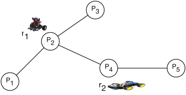
Figure 5: A Multi-Agent Path Finding Problem

It is easy to see that a MAPF $\mathcal{M}=(R,(V,E),s,d)$ can be represented by

• a set $\{\mathcal{P}_{r}\mid r\in R\}$ of path-planning problems for the robots in $R$, where for each $r\in R$, $\mathcal{P}_{r}=\langle D_{r},at(r,s(r)),at(r,d(r))\rangle$ is a planning problem with

  $$D_{r}=\left\{\begin{array}[]{lll}\hbox{\bf causes}(move(r,l,l^{\prime}),at(r,l^{\prime}),\{at(r,l)\})&&\mbox{ for }(l,l^{\prime})\in E\\ \hbox{\bf caused}(\{at(r,l)\},\neg at(r,l^{\prime}))\}&&\mbox{ for }l\neq l^{\prime},l,l^{\prime}\in V\\ \end{array}\right.$$

• the set of constraints representing the collisions.

ASP-based solutions of MAPF problems have been proposed for both action-based as well as state-based encodings. In the context of this survey, we will focus on an action-based encoding. Consider a MAPF problem $\mathcal{M}=(R,(V,E),s,d)$. The program developed in Section 3 for a single-agent planning problem can be used to develop a program solving $\mathcal{M}$, denoted by $\Pi(\mathcal{M},n)$, as follows. $\Pi(\mathcal{M},n)$ contains the following groups of rules:

1. the set of atoms $\{agent(r)\mid r\in R\}$ encoding the robots;

2. the collection of the rules from $\Pi(\mathcal{P}_{r},n)$; and

3. the constraints to avoid collisions:

   $$\leftarrow agent(R),agent(R^{\prime}),R\neq R^{\prime},$$

   $$holds(at(R,V),T),holds(at(R^{\prime},V),T)$$

   $$\leftarrow agent(R),agent(R^{\prime}),R\neq R^{\prime},$$

   $$holds(at(R,V),T),holds(at(R^{\prime},V^{\prime}),T),$$

   $$holds(at(R,V^{\prime}),T+1),holds(at(R^{\prime},V),T+1)$$

Rule (3) prevents two robots to be at the same location at the same time, while rule (3) guarantees that edge-collisions will not occur. These two constraints and the correctness of $\Pi(\mathcal{P}_{r},n)$ imply that $\Pi(\mathcal{M},n)$ computes solutions of length $n$ for the MAPF problem $\mathcal{M}$.

The proposed method for solving MAPF problems can be generalized to multi-agent planning as considered by the multi-agent community in the setting discussed by Durfee (1999). We assume that a multi-agent planning problem $\mathcal{M}$ for a set of agents $R$ is specified by a pair $(\mathcal{P}_{r\in R},\mathcal{C})$ where $\mathcal{P}_{r}=\langle D_{r},\Delta_{r},\Gamma_{r}\rangle$ is the planning problem for agent $r$ and $\mathcal{C}$ is a set of global constraints. For simplicity of the presentation, we will assume that

• the agents in $R$ share the same set of fluents and, wherever needed, parameterized with the names of the agents; for example, if an agent is carrying something then $carrying(r,o)$ will be used instead of $carrying(o)$ as in a single-agent domain;

• the actions in the domain in $D_{r}$ are parameterized with the agent’s name $r$, e.g., we will use the action $move(r,l,l^{\prime})$ instead of the traditional encoding $move(l,l^{\prime})$;

• the constraints in $\mathcal{C}$ are of the form

  $$\hbox{\bf executable}(sa,\varphi)$$ (70)

  where $sa$ is a set of actions in $\bigcup_{r\in R}D_{r}$ and $\varphi$ is a set of literals. This can be used to represent parallel actions, non-concurrent actions, etc.

For a multi-agent planning problem $\mathcal{M}=(\mathcal{P}_{r\in R},\mathcal{C})$ where $\mathcal{P}_{r}=\langle D_{r},\Delta_{r},\Gamma_{r}\rangle$, the program $\Pi(\mathcal{M},n)$ that computes solution for $\mathcal{M}$ consists of

1. the set of agent declarations, $agent(r)$ for $r\in R$;

2. the collection of the rules from $\Pi(\mathcal{P}_{r},n)$ with the following modifications:

   • the action specification of the form $action(a)$ is replaced by $action(r,a)$;

   • the action generation rule is replaced by

     $$1\{occ(A,T):action(R,A)\}1\leftarrow time(T),agent(R)$$

   where, without the loss of generality, we assume that every $D_{r}$ contains the action noop that is always executable and has no effect;

3. for each constraint of form (70), we create a new “collective” action named $sa_{id}$, add $action(sa_{id})$ to the set of actions in $\mathcal{M}$ (and make the (70) its executability condition, translated into ASP as for any other action) and, for each $a\in sa$, the following rule is added to $\Pi(\mathcal{P}_{r},n)$:

   $$occ(a,T) \leftarrow occ(sa_{id},T)$$ (71)

8.2 Distributed Planning

A main drawback of centralized planning is that it cannot exploit the structural organization of agents (e.g., hierarchical organization of agents) in the planning process. Distributed planning has been proposed as an alternative to centralized planning that aims at exploiting the independence between agents and/or groups of agents. We discuss distributed planning in two settings: fully collaborative agents and partially-cooperative or non-cooperative agents.

8.2.1 Fully Collaborative Agents

When agents are fully collaborative, a possible way to exploit structural relationships between agents is to allow each group of agents to plan for itself (e.g., using the planning system described in Section 3 and then employ a centralized post-planning process (a.k.a. the controller/scheduler) to create the joint plan for all agents. The controller takes the output of these planners—individual plans—and merges them into an overall plan. One of the main tasks of the controller is to resolve conflicts between individual plans. This issue arises because individual groups plan without knowledge of other groups (e.g., robot $r_{1}$ does not know the location of robot $r_{2}$). When the controller is unable to resolve all possible conflicts, the controller will identify plans that need to be changed and request different individual plans from specific individual groups.

Any implementation of distributed planning requires some communication capabilities between the controller and the individual planning systems. For this reason, a client-server architecture is often employed in the implementation of distributed planning. A client plans for an individual group of agents and the server is responsible for merging the individual plans from all groups. Although specialized parallel ASP solvers exist (e.g., the systems discussed in the papers by Le and Pontelli (2005) and Schneidenbach et al. (2009)), there has been no attempt to use parallel ASP solvers in distributed planning. Rather, distributed planning using ASP has been implemented using a combination of Prolog and ASP, where communication between server and clients is achieved through Prolog-based message passing, and planning is done using ASP (e.g., the system described in the paper by Son et al. (2009)).

Observe that the task of resolving conflicts is not straightforward and can require multiple iterations with individual planner(s) before the controller can create a joint plan. Consider again the two robots in Figure 5. If they are to generate their own plans, then the first set of individual solutions can be

$${\begin{array}[]{l}occ(move(r_{1},p_{2},p_{4}),0),occ(move(r_{1},p_{4},p_{5}),1)\end{array}}$$ (72)

and

$${\begin{array}[]{l}occ(move(r_{2},p_{4},p_{2}),0),occ(move(r_{2},p_{2},l_{3}),1)\end{array}}$$ (73)

A parallel execution of these two plans will result in a violation of the constraint stating that two robots cannot be at the same location at the same time. One can see that the controller needs to insert a few actions into both plans (e.g., $r_{1}$ must move to either $l_{1}$ or $l_{3}$ before moving to $l_{4}$).

Let $\mathcal{M}$ be a multi-agent planning problem and $P_{\{r\in R\}}$ be the plans received by the controller. The feasibility of merging these plans into a single plan for all agents can be checked using ASP. Let $\pi_{n}$ be the program obtained from $\Pi(\mathcal{M},n)$ (described in Subsection 8.1) by adding to $\Pi(\mathcal{M},n)$

• the set of action occurrences in $P_{\{r\in R\}}$, i.e.,

  $$\bigcup_{\{r\in R\}}\{occurs(a,t)\mid occ(a,t)\in P_{r}\}$$

• for $r\in R$, rules mapping time steps from 0 to $n$ to time steps used in $P_{r}$ ($r\in R$),

  $$\begin{array}[]{l}1\{map(r,T,J):time(J)\}1\leftarrow time(T),T<n,T\leq\max_{r}\\ \leftarrow map(r,T,J),map(p,T^{\prime},J^{\prime}),T<T^{\prime},J>J^{\prime}\end{array}$$

  where $\max_{r}$ is the maximal index in $P_{r}$. Intuitively, $map(r,i,j)$ indicates that the $i^{th}$ action in $P_{r}$ should occur in the $j^{th}$ position in the joint plan. This mapping must conform to the order of action occurrences in $P_{r}$.

• a rule ensuring that an atom $occurs(a,j)\in P_{r}$ must occur at the specified position:

  $$\leftarrow occ(a,t),map(r,t,j),{not\>}occurs(a,j).$$

It can be checked that $\pi_{4}$ would generate an answer set consisting of

$$\begin{array}[]{l}occ(move(r_{1},p_{2},p_{1}),0),occ(move(r_{2},p_{4},p_{2}),0),\\ occ(move(r_{2},p_{2},l_{3}),1),occ(move(r_{1},p_{1},p_{2}),1),\\ occ(move(r_{1},p_{2},p_{1}),2),\\ occ(move(r_{2},p_{4},p_{2}),3)\end{array}$$

which corresponds to the mapping $map(1,0,2),map(1,1,3),map(2,0,0),map(2,1,1)$ and is a successful merge of the two plans in (72)–(73).

Observe that the program $\pi_{n}$ might have no answer sets, which indicates that the merging of the plans $P_{\{r\in R\}}$ is unsuccessful. For instance, $\pi_{3}$ has no answer set, i.e., the two plans in (72)–(73) cannot be merged with less than four steps.

8.2.2 Non/Partially-Collaborative Agents

Centralized planning or distributed planning with an overall controller is most suitable in applications with collaborative (or non-competitive) agents such as the robots in the MAPF problems. In many applications, this assumption does not hold, e.g., agents may need to withhold certain private information and thus do not want to share their information freely; or agents may be competitive and have conflicting goals. In these situations, distributed planning as described in the previous sub-section is not applicable and planning will have to rely on a message passing architecture, e.g., via peer-to-peer communications. Furthermore, an online planning approach might be more appropriate. Next, we describe an ASP approach that is implemented centrally by Son et al. (2009) but could also be implemented distributedly.

In this approach, the planning process is interleaved with a negotiation process among agents. As an example, consider the robots in Figure 5 and assume that the robots can communicate with each other, but they cannot reveal their location. The following negotiation between $r_{2}$ and $r_{1}$ could take place:

• $r_{2}$ (to $r_{1}$): “can you ($r_{1}$) move out of $l_{2}$, $l_{3}$, and $l_{4}$?” (because $r_{2}$ needs to make sure that it can move to location $l_{2}$ and $l_{3}$). This can be translated to the formula $\varphi_{1}=\neg at(r_{1},l_{2})\wedge\neg at(r_{1},l_{3})\wedge\neg at(r_{1},l_{4})$ sent from $r_{2}$ to $r_{1}$.

• $r_{1}$ (to $r_{2}$): “I can do so after two steps but I would also like for you ($r_{2}$) to move out of $l_{2}$, $l_{4}$, and $l_{5}$ after I move out of those places.” This means that $r_{1}$ agrees to satisfy the formula sent by $r_{2}$ but also has some conditions of its own. This can be represented by the formula $\varphi_{1}\supset\varphi_{2}=\neg at(r_{2},l_{2})\wedge\neg at(r_{2},l_{4})\wedge\neg at(r_{2},l_{5})$.

• $r_{2}$ (to $r_{1}$): “that is good; however, do not move through $l_{4}$ to get out of the area.”

• etc.

The negotiation will continue until either the agent accepts (or refutes) the latest proposal from the other agent. A formal ASP based negotiation framework (e.g., the system described by Son et al. (2014)) could be used for this purpose.

Observe that during a negotiation, none of the robots changes its location or executes any action. After a successful negotiation, each robot has some additional information to take into consideration in its planning. In this example, if the two robots agree after the second proposal by $r_{2}$, robot $r_{1}$ agrees to move out of $l_{2}$, $l_{3}$, and $l_{4}$ but should do so without passing by $l_{4}$; robot $r_{2}$ knows that he can have $l_{2}$, $l_{3}$, and $l_{4}$ for itself after sometime and also knows that it can stand at $l_{4}$ until $r_{1}$ is out of the requested area; etc. Note, however, that this is not yet sufficient for the two robots to achieve their goals. To do so, they also need to agree on the timing of their moves. For example, $r_{1}$ can tell $r_{2}$ that $l_{2}$, $l_{3}$, and $l_{4}$ will be free after two steps; $r_{2}$ responds that, if it is the case, then $l_{2}$, $l_{4}$, and $l_{5}$ will be free after 2 steps; etc. This information will help the robots come up with plans for their own goals.

To the best of our knowledge, only a prototype implementation of the approach to interleaving negotiation and planning has been presented Son et al. (2009). It is also not implemented distributedly.

Remark 7

1. There are two different ways to enforce the collision-free constraint in the MAPF encoding. One can, for example, replace (3) with the rule

   $$\begin{array}[]{rcl}&\leftarrow&agent(R),agent(R^{\prime}),R\neq R^{\prime},\\ &&holds(at(R,V),T),holds(at(R^{\prime},V^{\prime}),T),\\ &&occ(move(R,V,V^{\prime}),T),occ(move(R^{\prime},V^{\prime},V),T+1)\end{array}$$

2. ASP-based solutions for various extensions of the MAPF problems have been discussed by Nguyen et al. (2017) and Gómez et al. (2020). The encoding proposed by Gómez et al. (2020) is special in that its grounded program has a linear size to the number of agents. An ASP-based solution for this problem has been applied in a real-world application Gebser et al. (2018). An environment for experimenting with MAPF has been developed by Gebser et al. (2018). A preliminary implementation of a MAPF solver on distributed platform can be found in the paper by Pianpak et al. (2019).

3. We observe that little attention has been paid to answer set programming based distributed planning. This also holds for the answer set programming based distributed computing platforms. Perhaps the need to attack problems in multi-agent systems will eventually lead to a truly distributed platform that could push the investigation of using answer set programming in this research direction to the next level. We note that the need for such platform exists and ad-hoc combinations with other programming language have been developed by Le et al. (2015).

8.3 Context: Planning in Multi-Agent Environments

Planning in multi-agent environments has been extensively investigated by the multi-agent research community. There exists a broad literature in this direction which addresses several issues, such as coordination, sharing of resources, use of shared resources, execution of joint actions, centralized or distributed computation of plans, sharing of tasks, etc. Earlier works in multi-agent planning (e.g., see the papers Allen and Zilberstein (2009); Brafman and Domshlak (2008); Bernstein et al. (2002); Brenner (2003); Crosby et al. (2014); Durfee (1999); de Weerdt et al. (2003); de Weerdt and Clement (2009); Goldman and Zilberstein (2004); Guestrin et al. (2001); Nair et al. (2003); Nissim and Brafman (2012); Peshkin and Savova (2002); Shoham and Leyton-Brown (2009); Torreño et al. (2012); Vlassis (2007)) focus on generating plans for multiple agents, coordinating the execution of plans, and does not take into consideration knowledge, beliefs, or privacy of agents. Work in planning for multiple self-interested agents can be found in the papers Gmytrasiewicz and Doshi (2005); Rathnasabapathy et al. (2006); Poupart and Boutilier (2003); Sonu and Doshi (2015).

The planning problem in multi-agent environments discussed in this section focuses on the setting in which each agent has its own goal, similar to the setting discussed in earlier work on multi-agent planning. It should be noted that MAPF has attracted a lot of attention in recent years due to its widespread applicability such as in warehouse or airtraffic control, leading to the organization of the yearly MAPF workshop at IJCAI and/or ICAPS conferences and several tutorials on the topic. A good description of this problem can be found in the papers Barták et al. (2019); Stern et al. (2019). Challenges and opportunities in MAPF and its extensions have been described by Salzman and Stern (2020). As with planning, search-based approaches to solving MAPF are frequently used. Early MAPF solvers, such as the ones described in the papers Goldenberg et al. (2014); Wagner and Choset (2015); Sharon et al. (2015); Boyarski et al. (2015); Cohen et al. (2016); Wang and Botea (2011); Luna and Bekris (2011); de Wilde et al. (2014), can compute optimal, boundedly-suboptimal, or suboptimal solutions of MAPF. Erdem et al. (2013), Yu and LaValle (2016), and Surynek et al. (2016) applied answer set programming, mixed-integer programming, and satisfiability testing, respectively, to solve the original MAPF problem. Suboptimal solutions of MAPF using SAT is discussed by Surynek et al. (2018). Surynek (2019b) presents an SMT-based MAPF solver.

Several extensions of the MAPF problem have been introduced. Ma and Koenig (2016) generalize MAPF to combined Target Assignment and Path Finding (TAPF), where agents are partitioned into teams and each team is given a set of targets that they need to reach. MAPF with deadlines is introduced by Ma et al. (2018). Extensions of the MAPF problem with delay probabilities have been described by Ma et al. (2017). The answer set planning implementation by Nguyen et al. (2017) shows that TAPF can be efficiently solved by answer set planning in multi-agent environments.

Andreychuk et al. (2019) investigate MAPF with continuous time, which removes the assumption that transitions between nodes are uniform. Barták and Svancara (2019) present a SAT-based approach to deal with this extension, while Surynek (2019a) describe an SMT-based MAPF solver for MAPF with continuous time and geometric agents.

Atzmon et al. (2020) focus on the issue of unexpected delays of agents and introduce the notion of $k$-robust MAPF plan, which can still be successfully executed when at most $k$ delays happen. This paper also studies a probabilistic extension of $k$-robust MAPF plan, called $pk$-robots MAPF plan.

A more realistic version of MAPF, which allows agents to exchange packages and transfer payload, is considered by Ma et al. (2016). Discussion of the problems where robots have kinematic constraints can be found in the paper Hönig et al. (2016).

It is worth noting that all of the aforementioned approaches to solving MAPF are centralized. Pianpak et al. (2019) propose a distributed ASP-based MAPF solver. In a recent paper, Gómez et al. (2021) present a compact ASP encoding for solving optimal sum-of-cost MAPF that is competitive with other approaches.

9 Planning with Scheduling and Extensions of ASP

Research on applications of ASP planning has also given impulse to, and is intertwined with, work on extensions of ASP. Let us consider the scenario from the following example.

Example 10 (From the paper by Balduccini (2011))

In a typical scenario from the domain of industrial printing, orders for the printing of books or magazines are more or less continuously received by the print shop. Each order involves the execution of multiple jobs. First, the pages are printed on (possibly different) press sheets. The press sheets are often large enough to accommodate several (10 to 100) pages, and thus a suitable layout of the pages on the sheets must be found. Next, the press sheets are cut in smaller parts called signatures. The signatures are then folded into booklets whose page size equals the intended page size of the order. Finally the booklets are bound together to form the book or magazine to be produced. The decision process is made more complex by the fact that multiple models of devices may be capable of performing a job. Furthermore, many decisions have ramifications and inter-dependencies. For example, selecting a large press sheet would prevent the use of a small press. The underlying decision-making process is often called production planning. Another set of decisions deals with scheduling. Here one needs to determine when the various jobs will be executed using the devices available in the print shop. Multiple devices of the same model may be available, thus even competing jobs may be run in parallel. Conversely, some of the devices can be offline—or go suddenly offline while production is in progress – and the scheduler must work around that. Typically, one wants to find a schedule that minimizes the tardiness of the orders while giving priority to the more important orders. Since orders are received on a continuous basis, one needs to be able to update the schedule in an incremental fashion, in a way that causes minimal disruption to the production, and can satisfy rush orders, which need to be executed quickly and take precedence over the others. Similarly, the scheduler needs to react to sudden changes in the print shop, such as a device going offline during production. $\Diamond$

This problem involves a combination of planning, configuration (of the devices involved) and scheduling. While ASP can certainly be used to represent the problem, computation presents challenges. In particular, the presence of variables with large domains has a tendency to cause a substantial increase in the size of the grounding of ASP programs. Under these conditions, both the grounding process itself and the following solving algorithms may take an unacceptable amount of time and/or memory. Similar challenges have been encountered in the ASP encoding of planning problems with large number of actions and steps (see, e.g., the discussion by Son and Pontelli (2007)).

Various extensions of ASP have been proposed over time to overcome this challenge. Some approaches, e.g., in response to large planning problems, rely on the avoidance of grounding, as illustrated in systems with lazy grounding (see, e.g., the papers by Palù et al. (2009), Cat et al. (2015), and Taupe et al. (2019)) or on the use of top-down execution models (see, e.g., the papers by Bonatti et al. (2008) and Marple and Gupta (2013)). At the core of the attempts focused on combination of planning and scheduling is the integration of ASP with techniques from constraint solving; this approach enables the effective ability to handle variables with large domains (especially numerical) efficiently.

Elkabani et al. (2004) provided an initial exploration of the combination of answer set programming with constraint logic programming, mostly focused on supporting the introduction of aggregates in answer set programming. Baselice et al. (2005) were among the first to propose a methodology for achieving such an integration as a way to extend the capabilities of the answer set programming framework. In their approach, the syntax and semantics of ASP is extended to enable the encoding of numerical constraints within the ASP syntax. Mellarkod et al. (2008) and Gebser et al. (2009) proposed solvers that support variants of ASP defined along the lines of the approach by Baselice et al. (2005), and specific ASP and constraint solvers are modified and integrated. In particular, the approach discussed in the clingcon systems Ostrowski and Schaub (2012); Banbara et al. (2017) explores the integration of constraint solving techniques with techniques like clause learning and back-jumping.

Experimental results show that these approaches lead to increased scalability, enabling the efficient resolution of planning domains of larger size. Later research extends and generalizes the language Bartholomew and Lee (2013), increasing the efficiency of the resolution algorithms; these extensions have been eventually integrated in the mainstream clingo solver Gebser et al. (2016). Notably, its extension with difference constraints, viz. clingo[dl], is operationally used by Swiss Railway for routing and scheduling train networks Abels et al. (2019).

All of these approaches rely on a clear-box architecture Balduccini and Lierler (2013), i.e., an architecture where the ASP components of the algorithm and its constraint solving components are tightly integrated and modified specifically to interact with each other. A different approach is proposed by Balduccini (2009) and later extensions. In that line of research, the goal is to enable the reuse, without modifications, of existing ASP and constraint solving algorithms. The intuition is that such an arrangement allows one to employ the best solvers available and makes it easy to analyze the performance of different combinations of solvers on a given task. This enabled researchers to propose a black-box architecture (and, later, a more advanced gray-box architecture), where the ASP and the constraint solving components are unaware of each other and are connected only by a thin “upper layer” of the architecture, which is responsible for exchanging data between the components and triggering their execution. The architecture proposed by Balduccini and Lierler (2017) is illustrated in Figure 6. Intuitively, answer sets are computed first by an off-the-shelf ASP solver. Special atoms are gathered by the “upper layer” and translated into a constraint satisfaction problem, which is solved by an off-the-shelf constraint solver. Solutions to the overall problem correspond to pairs formed by an answer set and a solution to the constraint satisfaction problem extracted from that answer set.

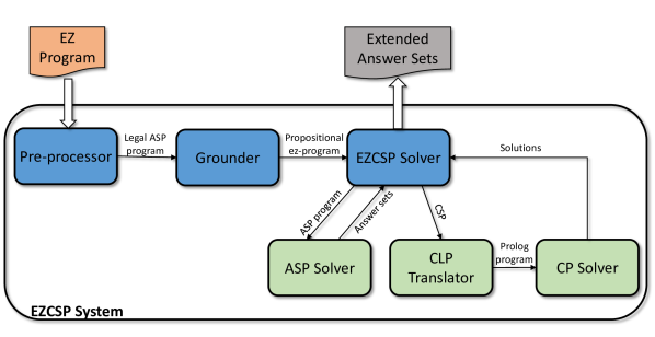
Figure 6: Architecture of the EZCSP solver Balduccini (2011)

This approach features an embedding of constraint solving constructs directly within the ASP language—that is, without the need to extend the syntax and semantics of ASP—by means of pre-interpreted relations known to the “upper layer” of the architecture (and some syntactic sugars for increased ease of formalization). For instance, constraint variables for the start time of jobs from Example 10 can be declared in the language described in the paper Balduccini (2011) by means of the rule

$$cspvar(st(D,J),0,MT)\leftarrow job(J),\ job\_device(J,D),max\_time(MT)$$ (74)

where $cspvar$ is a special relation that the “upper layer” knows how to translate into a variable declaration for a numerical constraint solver. Similarly, the effect on start times of precedences between jobs can be encoded by the ASP rule

$$\begin{array}[]{l}required(st(D2,J2)\geq st(D1,J1)+Len1)\leftarrow\\ \hskip 72.26999ptjob(J1),\ job(J2),\ job\_device(J1,D1),\ job\_device(J2,D2),\\ \hskip 72.26999ptprecedes(J1,J2),\ job\_len(J1,Len1)\end{array}$$ (75)

where “$\geq$” is a syntactic sugar for the predicate $at\_least$, written in the infix notation, and it is replaced by a pre-interpreted function symbol during pre-processing. As before, the “upper layer” is aware of the relation $required$ and translates the corresponding atoms to numerical constraints. A problem involving a combination of planning and scheduling such as that described in Example 10 can be elegantly and efficiently solved by extending a planning problem $\langle D,\Gamma,\Delta\rangle$ with statements such as (74) and (75).

Later research on this topic Balduccini and Lierler (2013, 2017) uncovered an interesting result: contrary to what one might expect, there is no clear winner in the performance comparison between black-box and white-box architectures (and gray-box as well); different classes of problems are more efficiently solved by a different architecture. Furthermore, Balduccini et al. (2017) showed that the EZCSP architecture can be used in planning with PDDL+ domains.

10 Conclusions and Future Directions

This paper surveys the progress made over the last 20+ years in the area of answer set planning. It focuses on the encoding in answer set programming of different classes of planning problems: when the initial state is complete, incomplete, and with or without sensing actions. In addition, the paper shows that answer set planning can reach the level of scalability and efficiency of state-of-the-art specialized planners, if useful information which can be exploited to guide the search process in planning, such as heuristics, is provided to the answer set solver. The paper also reviews some of the main research topics related to planning, such as planning with preferences, diagnosis, planning in multi-agent environments, and planning integrated with scheduling. We note that research related to answer set planning has been successfully applied in different application domains, often in combination with other types of reasoning, such as planning for the shuttle spacecraft by Nogueira et al. (2001), planning and scheduling Balduccini (2011), robotics Aker et al. (2011), scheduling Abels et al. (2019); Dodaro et al. (2019); Gebser et al. (2018), and multi-agent path findings Gómez et al. (2021); Nguyen et al. (2017). Section 9 also discusses the potential impacts that the use of answer set planning in real-world applications can have on the development of answer set programming.

In spite of this extensive body of research, there are still several challenges for answer set planning.

Performance of ASP Planning:

We note that extensive experimental comparisons with state-of-the-art compatible planning systems have been conducted. For example, Gebser et al. (2013) experimented with classical planning, Eiter et al. (2003b) and Tu et al. (2011) worked with incomplete information and non-deterministic actions, and Tu et al. (2007) with planning with sensing actions. The detailed comparisons can be found in the aforementioned papers and several other references that have been discussed throughout the paper. These comparisons demonstrate that ASP-planning is competitive with other approaches to planning, such as heuristic based planning or SAT-based planning.

The flexibility and expressiveness of answer set programming provide a simple way for answer set planning to exploit various forms of domain knowledge. To the best of our knowledge, no heuristic planning system can take advantages of all well-known types of domain knowledge, such as hierarchical structure, temporal knowledge, and procedural knowledge, whist they can be easily integrated into a single answer set planning system, as demonstrated by Son et al. (2006).

It is important to note that the performance of answer set planning systems depends heavily on the performance of the answer set solvers used in computing the solutions. As such, it is expected that these answer set planing systems can benefit from the advancements made by the ASP community. On the other hand, this hand-off approach also gives rise to limitations of ASP-based planning systems, such as scalability, heuristics, and ability to work with numeric values. It is worth noting that heuristics can be specified for guiding the answer set solver (e.g., as done by Gebser et al. (2013) in planning) and there are considerable efforts in integrating answer set solvers and constraint solvers (see Section 9). However, there exists no answer set planning system that works with PDDL+, similarly to the system SMTPlan by Cashmore et al. (2020) which employs SMT planning for hybrid systems described in PDDL+. An ASP-based planning system for PDDL+ is proposed by Balduccini et al. (2017). Yet, this system cannot deal with all features of PDDL+ as SMTPlan. The issue of numeric constraints is also related to the next challenge.

Probabilistic planning:

This research topic is the objective of intensive research within the automated planning community. Similarly to other planning paradigms, competitions among different probabilistic planning systems are organized within ICAPS (International Conference on Automated Planning and Scheduling, e.g., https://ipc2018-probabilistic.bitbucket.io/) and attract several research groups from academia and industry.

Probabilistic planning is concerned with identifying an optimal policy for an agent in a system specified by a Markov decision problem (MDP) or a Partial observable MDP (POMDP). While algorithms for computing an optimal policy are readily available (e.g., value iteration algorithm by Bellman (1957), topological value iteration by Dai et al. (2011), ILAO* by Hansen and Zilberstein (2001), LRTPD by Bonet and Geffner (2003), UCB by Kocsis and Szepesvári (2006), as well as the work of Kaelbling et al. (1998); the interested readers is also referred to the survey by Shani et al. (2013)), scalability and efficiency remain significant issues in this research area.

Computing MDP and POMPD in logic programming will be a significant challenge for ASP, due to the fact that answer set solvers are not developed to easily operate with real numbers. In addition, the exponential number of states of a MDP or POMPD require a representation language suitable for use with ASP. This challenge can be addressed using probabilistic action languages, such as the ones proposed by Baral et al. (2002) or by Wang and Lee (2019). On the other hand, working with real numbers means that the grounding-then-solving method to compute answer sets is no longer adequate. First of all, the presence of real numbers implies that the grounding process might not terminate. While discretization can be used to alleviate the grounding problem, it could increase the size of the grounded program significantly, creating problems (e.g., lack of memory) for the solving process. A potential approach to address these challenges is to integrate constraint solvers into answer set solvers, creating hybrid systems that can effectively deal with numeric constraints. Research in this direction has been summarized in Section 9. The recent implementation by Abels et al. (2019) demonstrates that answer set programming based system can work effectively with a huge number of numeric constraints.

Epistemic planning:

In recent years, epistemic multi-agent planning (EMP) has gained significant interest within the planning community. Löwe et al. (2011) propose a general epistemic planning framework. Complexity of EMP has been studied in the papers Aucher and Bolander (2013); Bolander et al. (2015); Charrier et al. (2016). Studies of EMP can be found in several papers Bolander and Andersen (2011); Engesser et al. (2017); van der Hoek and Wooldridge (2002); Huang et al. (2017); Löwe et al. (2011); Eijck (2004) and many planners have been developed Burigana et al. (2020); Fabiano et al. (2020); Le et al. (2018); Muise et al. (2015); Kominis and Geffner (2015, 2017); Wan et al. (2015). With the exception of the planner developed by Burigana et al. (2020), which employs answer set programming, the majority of the proposed systems are heuristic search based planners. Some EMP planners, such as those proposed by Muise et al. (2015), Kominis and Geffner (2015) and 2017, translate an EMP problem into a classical planning problem and use classical planners to find solutions.

A multi-agent planning problem of this type is different from the planning problems discussed in Section 8, in that it considers the knowledge and beliefs of agents, and explores the use of actions that manipulate such knowledge and beliefs. This is necessary for planning in non-collaborative and competitive environments. The difficulty in this task lies in that the result of the execution of an action (by an agent or a group of agents) will change the state of the world and the state of knowledge and belief of other agents. Inevitably, some agents may have false beliefs about the world. Semantically, the transitions from the state of affair, that includes the state of the world and the state of knowledge and beliefs of the agents, to another state of affair could be modeled by transitions between Kripke structures (see, e.g., the books Fagin et al. (1995); Van Ditmarsch et al. (2007)). A Kripke structure consists of a set of worlds and a set of binary accessibility relations over the worlds. A practical challenge is related to the size of the Kripke structures, in terms of the number of worlds—as this can double after the execution of each action. Intuitively, this requires the ability to generate new terms in the answer set solvers during resolution. Multi-shot solvers (see, e.g., the paper Gebser et al. (2019)) could provide a good platform for epistemic planning. Preliminary encouraging results on the use of answer set programming in this context have been recently presented by Burigana et al. (2020).

Explainable Planning (XAIP):

This is yet another problem that has only recently been investigated but attracted considerable attention from the planning community, leading to the organization of a a yearly workshop on XAIP associated with ICAPS (e.g., https://icaps20subpages.icaps-conference.org/workshops/xaip/). Several questions for XAIP are discussed by Fox et al. (2017). In XAIP, a human questions the planner (a robot’s planning system) about its proposed solution. The focus is on explaining why a planner makes a certain decision. For example, why an action is included (or not included) in the plan? Why is the proposed plan optimal? Why can a goal not be achieved? Why should (or should not) the human consider replanning?

Chakraborti et al. (2017), for example, describe model reconciliation problem (MRP) and propose methods for solving it. In a MRP, the human and the robot have their own planning problems. The goal in both problems are the same, but the action specifications and the initial states might be different. The robot generates an optimal plan and informs the human of its plan. The human declares that it is not an optimal plan according to their planning problem specification. The robot, which is aware of the human’s problem specification, needs to present to the human the reasons why its plan is optimal and what is wrong in the human’s problem specification. Often, the answer is in the form of a collection of actions, actions’ preconditions and effects, and literals from the initial states that should be added to, or removed from, the human’s problem specification so that the robot’s plan will be an optimal plan of the updated specification. While explanations have been extensively investigated by the logic programming community, explainable planning using answer set programming has been investigated only recently by Nguyen et al. (2020).

Acknowledgement

Tran Son and Enrico Pontelli have been partially supported by NSF grants 1914635, 1833630, 1757207, and 1812628. Tran Son’s and Marcello Balduccini’s contribution was made possible in part through the help and support of NIST via cooperative agreement 70NANB21H167. Torsten Schaub was supported by DFG grant SCHA 550/15, Germany.

References

- Abels et al. (2019) Abels, D., Jordi, J., Ostrowski, M., Schaub, T., Toletti, A., and Wanko, P. 2019. Train scheduling with hybrid ASP. In Proceedings of the Fifteenth International Conference on Logic Programming and Nonmonotonic Reasoning (LPNMR’19), M. Balduccini, Y. Lierler, and S. Woltran, Eds. Lecture Notes in Artificial Intelligence, vol. 11481. Springer-Verlag, 3–17.
- Aker et al. (2011) Aker, E., Erdogan, A., Erdem, E., and Patoglu, V. 2011. Causal reasoning for planning and coordination of multiple housekeeping robots. In Proceedings of the Eleventh International Conference on Logic Programming and Nonmonotonic Reasoning (LPNMR’11), J. Delgrande and W. Faber, Eds. Lecture Notes in Artificial Intelligence, vol. 6645. Springer-Verlag, 311–316.
- Albore et al. (2011) Albore, A., Ramírez, M., and Geffner, H. 2011. Effective heuristics and belief tracking for planning with incomplete information. In Proceedings of the Twenty-first International Conference on Automated Planning and Scheduling (ICAPS’11), F. Bacchus, C. Domshlak, S. Edelkamp, and M. Helmert, Eds. AAAI Press, 2–8.
- Allen et al. (1990) Allen, J., Hendler, J., and Tate, A., Eds. 1990. Readings in planning. Morgan Kaufmann, CA, USA.
- Allen et al. (1991) Allen, J., Kautz, H., Pelavin, R., and Tenenberg, J. 1991. Reasoning about plans. Morgan Kaufmann.
- Allen and Zilberstein (2009) Allen, M. and Zilberstein, S. 2009. Complexity of decentralized control: Special cases. In Proceedings of the Twenty-third Annual Conference on Neural Information Processing Systems (NIPS’09), Y. Bengio, D. Schuurmans, J. Lafferty, C. Williams, and A. Culotta, Eds. Curran Associates, Inc., 19–27.
- Alviano et al. (2017) Alviano, M., Calimeri, F., Dodaro, C., Fuscà, D., Leone, N., Perri, S., Ricca, F., Veltri, P., and Zangari, J. 2017. The ASP system DLV2. In Proceedings of the Fourteenth International Conference on Logic Programming and Nonmonotonic Reasoning (LPNMR’17), M. Balduccini and T. Janhunen, Eds. Lecture Notes in Artificial Intelligence, vol. 10377. Springer-Verlag, 215–221.
- Alviano et al. (2013) Alviano, M., Dodaro, C., Faber, W., Leone, N., and Ricca, F. 2013. WASP: A native ASP solver based on constraint learning. In Proceedings of the Twelfth International Conference on Logic Programming and Nonmonotonic Reasoning (LPNMR’13), P. Cabalar and T. Son, Eds. Lecture Notes in Artificial Intelligence, vol. 8148. Springer-Verlag, 54–66.
- Aminof et al. (2020) Aminof, B., De Giacomo, G., Lomuscio, A., Murano, A., and Rubin, S. 2020. Synthesizing strategies under expected and exceptional environment behaviors. In Proceedings of the Twenty-Ninth International Joint Conference on Artificial Intelligence (IJCAI’20), C. Bessiere, Ed. ijcai.org, 1674–1680.
- Andreychuk et al. (2019) Andreychuk, A., Yakovlev, K., Atzmon, D., and Stern, R. 2019. Multi-agent pathfinding with continuous time. In Proceedings of the Twenty-Eighth International Joint Conference on Artificial Intelligence (IJCAI’19), S. Kraus, Ed. ijcai.org, 39–45.
- Atzmon et al. (2020) Atzmon, D., Stern, R., Felner, A., Wagner, G., Barták, R., and Zhou, N. 2020. Robust multi-agent path finding and executing. Journal of Artificial Intelligence Research 67, 549–579.
- Aucher and Bolander (2013) Aucher, G. and Bolander, T. 2013. Undecidability in epistemic planning. In Proceedings of the Twenty-third International Joint Conference on Artificial Intelligence (IJCAI’13), F. Rossi, Ed. IJCAI/AAAI Press, 27–33.
- Bacchus (2001) Bacchus, F. 2001. The AIPS’00 planning competition. AI Magazine 22, 3, 47–56.
- Bäckström and Nebel (1995) Bäckström, C. and Nebel, B. 1995. Complexity results for SAS+ planning. Computational Intelligence 11, 625–656.
- Baier and McIlraith (2008) Baier, J. and McIlraith, S. 2008. Planning with preferences. AI Magazine 29, 4, 25–36.
- Balduccini (2009) Balduccini, M. 2009. Representing constraint satisfaction problems in answer set programming. In Proceedings of the Second Workshop on Answer Set Programming and Other Computing Paradigms (ASPOCP’09), W. Faber and J. Lee, Eds. 16–30.
- Balduccini (2011) Balduccini, M. 2011. Industrial-size scheduling with ASP+CP. In Proceedings of the Eleventh International Conference on Logic Programming and Nonmonotonic Reasoning (LPNMR’11), J. Delgrande and W. Faber, Eds. Lecture Notes in Artificial Intelligence, vol. 6645. Springer-Verlag, 284–296.
- Balduccini and Gelfond (2003) Balduccini, M. and Gelfond, M. 2003. Diagnostic reasoning with A-Prolog. Theory and Practice of Logic Programming 3, 4-5, 425–461.
- Balduccini and Lierler (2013) Balduccini, M. and Lierler, Y. 2013. Integration schemas for constraint answer set programming: a case study. In Technical Communications of the Twenty-ninth International Conference on Logic Programming (ICLP’13), E. Lamma and T. Swift, Eds. Theory and Practice of Logic Programming, Online Supplement, vol. 13(4-5).
- Balduccini and Lierler (2017) Balduccini, M. and Lierler, Y. 2017. Constraint answer set solver EZCSP and why integration schemas matter. Theory and Practice of Logic Programming 17, 4, 462–515.
- Balduccini et al. (2017) Balduccini, M., Magazzeni, D., Maratea, M., and Leblanc, E. 2017. CASP solutions for planning in hybrid domains. Theory and Practice of Logic Programming 17, 4, 591–633.
- Banbara et al. (2017) Banbara, M., Kaufmann, B., Ostrowski, M., and Schaub, T. 2017. Clingcon: The next generation. Theory and Practice of Logic Programming 17, 4, 408–461.
- Baral and Gelfond (2000) Baral, C. and Gelfond, M. 2000. Reasoning agents in dynamic domains. In Logic-Based Artificial Intelligence, J. Minker, Ed. Kluwer Academic Publishers, Dordrecht, 257–279.
- Baral et al. (2000) Baral, C., Kreinovich, V., and Trejo, R. 2000. Computational complexity of planning and approximate planning in the presence of incompleteness. Artificial Intelligence 122, 1-2, 241–267.
- Baral et al. (2000) Baral, C., McIlraith, S., and Son, T. 2000. Formulating diagnostic problem solving using an action language with narratives and sensing. In Proceedings of the Seventh International Conference on Principles of Knowledge Representation and Reasoning (KR’00), A. Cohn, F. Giunchiglia, and B. Selman, Eds. Morgan Kaufmann Publishers, 311–322.
- Baral et al. (2002) Baral, C., Nam, T., and Tuan, L. 2002. Reasoning about actions in a probabilistic setting. In Proceedings of the Eighteenth National Conference on Artificial Intelligence (AAAI’02), R. Dechter, M. Kearns, and R. Sutton, Eds. AAAI Press, 507–512.
- Baroni et al. (1999) Baroni, P., Lamperti, G., Pogliano, P., and Zanella, M. 1999. Diagnosis of large active systems. Artificial Intelligence 110, 1, 135–183.
- Barták and Svancara (2019) Barták, R. and Svancara, J. 2019. On sat-based approaches for multi-agent path finding with the sum-of-costs objective. In Proceedings of the Twelfth International Symposium on Combinatorial Search (SOCS’19), P. Surynek and W. Yeoh, Eds. AAAI Press, 10–17.
- Barták et al. (2019) Barták, R., Svancara, J., Skopková, V., Nohejl, D., and Krasicenko, I. 2019. Multi-agent path finding on real robots. AI Magazine 32, 3, 175–189.
- Bartholomew and Lee (2013) Bartholomew, M. and Lee, J. 2013. Functional stable model semantics and answer set programming modulo theories. In Proceedings of the Twenty-third International Joint Conference on Artificial Intelligence (IJCAI’13), F. Rossi, Ed. IJCAI/AAAI Press, 718–724.
- Baselice et al. (2005) Baselice, S., Bonatti, P., and Gelfond, M. 2005. Towards an integration of answer set and constraint solving. In Proceedings of the Twenty-first International Conference on Logic Programming (ICLP’05), M. Gabbrielli and G. Gupta, Eds. Lecture Notes in Computer Science, vol. 3668. Springer-Verlag, 52–66.
- Bellman (1957) Bellman, R. 1957. A markovian decision process. Journal of Mathematics and Mechanics 6, 5, 679–684.
- Bernstein et al. (2002) Bernstein, D., Givan, R., Immerman, N., and Zilberstein, S. 2002. The complexity of decentralized control of markov decision processes. Mathematics of Operations Research 27, 4, 819–840.
- Bidoux et al. (2019) Bidoux, L., Pignon, J., and Bénaben, F. 2019. Planning with preferences using multi-attribute utility theory along with a choquet integral. Engineering Applications of Artificial Intelligence 85, 808–817.
- Blum and Furst (1997) Blum, A. and Furst, M. 1997. Fast planning through planning graph analysis. Artificial Intelligence 90, 1-2, 281–300.
- Bolander and Andersen (2011) Bolander, T. and Andersen, M. 2011. Epistemic planning for single and multi-agent systems. Journal of Applied Non-Classical Logics 21, 1, 9–34.
- Bolander et al. (2015) Bolander, T., Jensen, M., and Schwarzentruber, F. 2015. Complexity results in epistemic planning. In Proceedings of the Twenty-fourth International Joint Conference on Artificial Intelligence (IJCAI’15), Q. Yang and M. Wooldridge, Eds. AAAI Press, 2791–2797.
- Bonatti et al. (2008) Bonatti, P., Pontelli, E., and Son, T. 2008. Credulous resolution for answer set programming. In Proceedings of the Twenty-third National Conference on Artificial Intelligence (AAAI’08), D. Fox and C. Gomes, Eds. AAAI Press, 418–423.
- Bonet and Geffner (2000) Bonet, B. and Geffner, H. 2000. Planning with incomplete information as heuristic search in belief space. In Proceedings of the Fifth International Conference on Artificial Intelligence Planning Systems (AIPS’00), S. Chien, S. Kambhampati, and C. Knoblock, Eds. AAAI Press, 52–61.
- Bonet and Geffner (2001) Bonet, B. and Geffner, H. 2001. Planning as heuristic search. Artificial Intelligence 129, 5–33.
- Bonet and Geffner (2003) Bonet, B. and Geffner, H. 2003. Labeled RTDP: improving the convergence of real-time dynamic programming. E. Giunchiglia, N. Muscettola, and D. Nau, Eds. AAAI Press, 12–21.
- Bonet and Helmert (2010) Bonet, B. and Helmert, M. 2010. Strengthening landmark heuristics via hitting sets. In Proceedings of the Nineteenth European Conference on Artificial Intelligence (ECAI’10), H. Coelho, R. Studer, and M. Wooldridge, Eds. IOS Press, 329–334.
- Boyarski et al. (2015) Boyarski, E., Felner, A., Stern, R., Sharon, G., Tolpin, D., Betzalel, O., and Shimony, S. 2015. ICBS: Improved conflict-based search algorithm for multi-agent pathfinding. In Proceedings of the Twenty-fourth International Joint Conference on Artificial Intelligence (IJCAI’15), Q. Yang and M. Wooldridge, Eds. AAAI Press, 740–746.
- Brafman and Domshlak (2008) Brafman, R. and Domshlak, C. 2008. From one to many: Planning for loosely coupled multi-agent systems. In Proceedings of the Eighteenth International Conference on Automated Planning and Scheduling (ICAPS’08), J. Rintanen, B. Nebel, J. Beck, and E. Hansen, Eds. AAAI Press, 28–35.
- Brafman and Hoffmann (2004) Brafman, R. and Hoffmann, J. 2004. Conformant planning via heuristic forward search: A new approach. In Proceedings of the Fourteenth International Conference on Automated Planning and Scheduling (ICAPS’04), S. Zilberstein, J. Koehler, and S. Koenig, Eds. AAAI Press, 355–364.
- Brenner (2003) Brenner, M. 2003. A multiagent planning language. In Proceedings of the Workshop on PDDL. 33–38.
- Brewka (2002) Brewka, G. 2002. Logic programming with ordered disjunction. In Proceedings of the Eighteenth National Conference on Artificial Intelligence (AAAI’02), R. Dechter, M. Kearns, and R. Sutton, Eds. AAAI Press, 100–105.
- Brewka et al. (2015a) Brewka, G., Delgrande, J., Romero, J., and Schaub, T. 2015a. asprin: Customizing answer set preferences without a headache. In Proceedings of the Twenty-Ninth National Conference on Artificial Intelligence (AAAI’15), B. Bonet and S. Koenig, Eds. AAAI Press, 1467–1474.
- Brewka et al. (2015b) Brewka, G., Delgrande, J., Romero, J., and Schaub, T. 2015b. Implementing preferences with asprin. In Proceedings of the Thirteenth International Conference on Logic Programming and Nonmonotonic Reasoning (LPNMR’15), F. Calimeri, G. Ianni, and M. Truszczyński, Eds. Lecture Notes in Artificial Intelligence, vol. 9345. Springer-Verlag, 158–172.
- Bryant (1992) Bryant, R. 1992. Symbolic boolean manipulation with ordered binary-decision diagrams. ACM Computing Surveys 24, 3, 293–318.
- Bryce et al. (2006) Bryce, D., Kambhampati, S., and Smith, D. 2006. Planning graph heuristics for belief space search. Journal of Artificial Intelligence Research 26, 35–99.
- Burigana et al. (2020) Burigana, A., Fabiano, F., Dovier, A., and Pontelli, E. 2020. Modelling multi-agent epistemic planning in ASP. Theory and Practice of Logic Programming 20, 5, 593–608.
- Calimeri et al. (2019) Calimeri, F., Faber, W., Gebser, M., Ianni, G., Kaminski, R., Krennwallner, T., Leone, N., Maratea, M., Ricca, F., and Schaub, T. 2019. ASP-Core-2 input language format. Theory and Practice of Logic Programming 20, 2, 294–309.
- Camacho et al. (2018) Camacho, A., Baier, J., Muise, C., and McIlraith, S. 2018. Finite LTL synthesis as planning. In Proceedings of the Twenty-eighth International Conference on Automated Planning and Scheduling (ICAPS’18), M. de Weerdt, S. Koenig, G. Röger, and M. Spaan, Eds. AAAI Press, 29–38.
- Camacho et al. (2019) Camacho, A., Bienvenu, M., and McIlraith, S. 2019. Towards a unified view of AI planning and reactive synthesis. In Proceedings of the Twenty-ninth International Conference on Automated Planning and Scheduling (ICAPS’19), J. Benton, N. Lipovetzky, E. Onaindia, D. Smith, and S. Srivastava, Eds. AAAI Press, 58–67.
- Cashmore et al. (2020) Cashmore, M., Magazzeni, D., and Zehtabi, P. 2020. Planning for hybrid systems via satisfiability modulo theories. Journal of Artificial Intelligence Research 67, 235–283.
- Castellini et al. (2003) Castellini, C., Giunchiglia, E., and Tacchella, A. 2003. SAT-based planning in complex domains: Concurrency, constraints and nondeterminism. Artificial Intelligence 147, 1-2, 85–117.
- Cat et al. (2015) Cat, B. D., Denecker, M., Bruynooghe, M., and Stuckey, P. 2015. Lazy model expansion: Interleaving grounding with search. Journal of Artificial Intelligence Research 52, 235–286.
- Chakraborti et al. (2017) Chakraborti, T., Sreedharan, S., Zhang, Y., and Kambhampati, S. 2017. Plan explanations as model reconciliation: Moving beyond explanation as soliloquy. In Proceedings of the Twenty-sixth International Joint Conference on Artificial Intelligence (IJCAI’17), C. Sierra, Ed. IJCAI/AAAI Press, 156–163.
- Charrier et al. (2016) Charrier, T., Maubert, B., and Schwarzentruber, F. 2016. On the impact of modal depth in epistemic planning. In Proceedings of the Twenty-fifth International Joint Conference on Artificial Intelligence (IJCAI’16), R. Kambhampati, Ed. IJCAI/AAAI Press, 1030–1036.
- Chen et al. (2009) Chen, Y., Huang, R., Xing, Z., and Zhang, W. 2009. Long-distance mutual exclusion for planning. Artificial Intelligence 173, 2, 365–391.
- Cimatti and Roveri (2000) Cimatti, A. and Roveri, M. 2000. Conformant planning via symbolic model checking. Journal of Artificial Intelligence Research 13, 305–338.
- Cimatti et al. (2004) Cimatti, A., Roveri, M., and Bertoli, P. 2004. Conformant planning via symbolic model checking and heuristic search. Artificial Intelligence 159, 1-2, 127–206.
- Cohen et al. (2016) Cohen, L., Uras, T., Kumar, T., Xu, H., Ayanian, N., and Koenig, S. 2016. Improved solvers for bounded-suboptimal multi-agent path finding. In Proceedings of the Twenty-fifth International Joint Conference on Artificial Intelligence (IJCAI’16), R. Kambhampati, Ed. IJCAI/AAAI Press, 3067–3074.
- Coles and Coles (2011) Coles, A. and Coles, A. 2011. LPRPG-P: relaxed plan heuristics for planning with preferences. In Proceedings of the Twenty-first International Conference on Automated Planning and Scheduling (ICAPS’11), F. Bacchus, C. Domshlak, S. Edelkamp, and M. Helmert, Eds. AAAI Press.
- Cordier and Thiébaux (1994) Cordier, M. and Thiébaux, S. 1994. Event-based diagnosis for evolutive systems. Tech. rep., Technical Report 819, IRISA, Cedex, France.
- Crosby et al. (2014) Crosby, M., Jonsson, A., and Rovatsos, M. 2014. A single-agent approach to multiagent planning. In Proceedings of the Twenty-first European Conference on Artificial Intelligence (ECAI’14), T. Schaub, G. Friedrich, and B. O’Sullivan, Eds. IOS Press, 237–242.
- Dai et al. (2011) Dai, P., Mausam, Weld, D., and Goldsmith, J. 2011. Topological value iteration algorithms. Journal of Artificial Intelligence Research 42, 181–209.
- Das et al. (2019) Das, M., Odom, P., Islam, M., Doppa, J., Roth, D., and Natarajan, S. 2019. Planning with actively eliciting preferences. Knowledge Based Systems 165, 219–227.
- De Kleer and Kurien (2003) De Kleer, J. and Kurien, J. 2003. Fundamentals of model-based diagnosis. IFAC Proceedings 36, 5, 25–36.
- de Weerdt et al. (2003) de Weerdt, M., Bos, A., Tonino, H., and Witteveen, C. 2003. A resource logic for multi-agent plan merging. Annals of Mathematics and Artificial Intelligence 37, 1-2, 93–130.
- de Weerdt and Clement (2009) de Weerdt, M. and Clement, B. 2009. Introduction to planning in multiagent systems. Multiagent and Grid Systems 5, 4, 345–355.
- de Wilde et al. (2014) de Wilde, B., ter Mors, A., and Witteveen, C. 2014. Push and rotate: a complete multi-agent pathfinding algorithm. Journal of Artificial Intelligence Research 51, 443–492.
- Denecker et al. (1992) Denecker, M., Missiaen, L., and Bruynooghe, M. 1992. Temporal reasoning with abductive event calculus. In Proceedings of the Tenth European Conference on Artificial Intelligence (ECAI’92), B. Neumann, Ed. John Wiley & sons, 384–388.
- Dimopoulos et al. (2019) Dimopoulos, Y., Gebser, M., Lühne, P., Romero, J., and Schaub, T. 2019. plasp 3: Towards effective ASP planning. Theory and Practice of Logic Programming 19, 3, 477–504.
- Dimopoulos et al. (1997) Dimopoulos, Y., Nebel, B., and Köhler, J. 1997. Encoding planning problems in nonmonotonic logic programs. In Proceedings of the Fourth European Conference on Planning, S. Steel and R. Alami, Eds. Lecture Notes in Artificial Intelligence, vol. 1348. Springer-Verlag, 169–181.
- Dix et al. (2005) Dix, J., Kuter, U., and Nau, D. 2005. Planning in answer set programming using ordered task decomposition. In We Will Show Them! Essays in Honour of Dov Gabbay, S. Artëmov, H. Barringer, A. d’Avila Garcez, L. Lamb, and J. Woods, Eds. Vol. 1. College Publications, 521–576.
- Do and Kambhampati (2003) Do, M. and Kambhampati, S. 2003. Sapa: A multi-objective metric temporal planner. Journal of Artificial Intelligence Research 20, 155–194.
- Dodaro et al. (2019) Dodaro, C., Galatà, G., Khan, M., Maratea, M., and Porro, I. 2019. An asp-based solution for operating room scheduling with beds management. P. Fodor, M. Montali, D. Calvanese, and D. Roman, Eds. Lecture Notes in Computer Science, vol. 11784. Springer-Verlag, 67–81.
- Dovier et al. (2009) Dovier, A., Formisano, A., and Pontelli, E. 2009. An empirical study of constraint logic programming and answer set programming solutions of combinatorial problems. Journal of Experimental and Theoretical Artificial Intelligence 21, 2, 79–121.
- Durfee (1999) Durfee, E. 1999. Distributed problem solving and planning. In Muliagent Systems: A Modern Approach to Distributed Artificial Intelligence, G. Weiss, Ed. MIT Press, 121–164.
- Eijck (2004) Eijck, J. v. 2004. Dynamic epistemic modelling. Tech. rep.
- Eiter et al. (2000) Eiter, T., Faber, W., Leone, N., Pfeifer, G., and Polleres, A. 2000. Planning under incomplete knowledge. In Proceedings of the First International Conference on Computational Logic (CL’00), J. Lloyd, V. Dahl, U. Furbach, M. Kerber, K. Lau, C. Palamidessi, L. Pereira, Y. Sagiv, and P. Stuckey, Eds. Lecture Notes in Computer Science, vol. 1861. Springer-Verlag, 807–821.
- Eiter et al. (2003a) Eiter, T., Faber, W., Leone, N., Pfeifer, G., and Polleres, A. 2003a. Answer set planning under action costs. Journal of Artificial Intelligence Research 19, 25–71.
- Eiter et al. (2003b) Eiter, T., Faber, W., Leone, N., Pfeifer, G., and Polleres, A. 2003b. A logic programming approach to knowledge-state planning. Artificial Intelligence 144, 1-2, 157–211.
- Eiter et al. (2004) Eiter, T., Faber, W., Leone, N., Pfeifer, G., and Polleres, A. 2004. A logic programming approach to knowledge-state planning: Semantics and complexity. ACM Transactions on Computational Logic 5, 2, 206–263.
- Eiter et al. (1997) Eiter, T., Leone, N., Mateis, C., Pfeifer, G., and Scarcello, F. 1997. A deductive system for nonmonotonic reasoning. In Proceedings of the Fourth International Conference on Logic Programming and Nonmonotonic Reasoning (LPNMR’97), J. Dix, U. Furbach, and A. Nerode, Eds. Lecture Notes in Artificial Intelligence, vol. 1265. Springer-Verlag, 363–374.
- Elkabani et al. (2004) Elkabani, I., Pontelli, E., and Son, T. 2004. Smodels with CLP and its applications: A simple and effective approach to aggregates in ASP. In Proceedings of the Twentieth International Conference on Logic Programming (ICLP’04), B. Demoen and V. Lifschitz, Eds. Lecture Notes in Computer Science, vol. 3132. Springer-Verlag, 73–89.
- Endriss et al. (2004) Endriss, U., Mancarella, P., Sadri, F., Terreni, G., and Toni, F. 2004. The CIFF proof procedure for abductive logic programming with constraints. In Proceedings of the Ninth European Conference on Logics in Artificial Intelligence (JELIA’04), J. Alferes and J. Leite, Eds. Lecture Notes in Computer Science, vol. 3229. Springer-Verlag, 31–43.
- Engesser et al. (2017) Engesser, T., Bolander, T., Mattmüller, R., and Nebel, B. 2017. Cooperative epistemic multi-agent planning for implicit coordination. In Proceedings of the Ninth Workshop on Methods for Modalities, S. Ghosh and R. Ramanujam, Eds. EPTCS, vol. 243. 75–90.
- Erdem et al. (2013) Erdem, E., Kisa, D., Öztok, U., and Schüller, P. 2013. A general formal framework for pathfinding problems with multiple agents. In Proceedings of the Twenty-Seventh National Conference on Artificial Intelligence (AAAI’13), M. desJardins and M. Littman, Eds. AAAI Press, 290–296.
- Eshghi (1988) Eshghi, K. 1988. Abductive planning with event calculus. In Proceedings of the Fifth International Conference on Logic Programming (ICLP’88), R. Kowalski and K. Bowen, Eds. MIT Press, 562–579.
- Fabiano et al. (2020) Fabiano, F., Burigana, A., Dovier, A., and Pontelli, E. 2020. EFP 2.0: A multi-agent epistemic solver with multiple e-state representations. In Proceedings of the Thirtieth International Conference on Automated Planning and Scheduling (ICAPS’20), J. Beck, O. Buffet, J. Hoffmann, E. Karpas, and S. Sohrabi, Eds. AAAI Press, 101–109.
- Fagin et al. (1995) Fagin, R., Halpern, J., Moses, Y., and Vardi, M. 1995. Reasoning About Knowledge. MIT Press.
- Fandinno et al. (2021) Fandinno, J., Laferriere, F., Romero, J., Schaub, T., and Son, T. 2021. Planning with incomplete information in quantified answer set programming. Theory and Practice of Logic Programming 21, 5, 663–679.
- Feldman et al. (2020) Feldman, A., Pill, I., Wotawa, F., Matei, I., and de Kleer, J. 2020. Efficient model-based diagnosis of sequential circuits. In Proceedings of the Thirty-fourth National Conference on Artificial Intelligence (AAAI’20). AAAI Press, 2814–2821.
- Fikes and Nilsson (1971) Fikes, R. and Nilsson, N. 1971. STRIPS: A new approach to the application of theorem proving to problem solving. Artificial Intelligence 2, 3-4, 189–208.
- Fox et al. (2017) Fox, M., Long, D., and Magazzeni, D. 2017. Explainable planning. CoRR abs/1709.10256.
- Gebser et al. (2015) Gebser, M., Kaminski, R., Kaufmann, B., Lindauer, M., Ostrowski, M., Romero, J., Schaub, T., and Thiele, S. 2015. Potassco User Guide, 2 ed. University of Potsdam.
- Gebser et al. (2016) Gebser, M., Kaminski, R., Kaufmann, B., Ostrowski, M., Schaub, T., and Wanko, P. 2016. Theory solving made easy with clingo 5. In Technical Communications of the Thirty-second International Conference on Logic Programming (ICLP’16), M. Carro and A. King, Eds. OpenAccess Series in Informatics (OASIcs), vol. 52. Schloss Dagstuhl–Leibniz-Zentrum fuer Informatik, 2:1–2:15.
- Gebser et al. (2019) Gebser, M., Kaminski, R., Kaufmann, B., and Schaub, T. 2019. Multi-shot ASP solving with clingo. Theory and Practice of Logic Programming 19, 1, 27–82.
- Gebser et al. (2007) Gebser, M., Kaufmann, B., Neumann, A., and Schaub, T. 2007. clasp: A conflict-driven answer set solver. In Proceedings of the Ninth International Conference on Logic Programming and Nonmonotonic Reasoning (LPNMR’07), C. Baral, G. Brewka, and J. Schlipf, Eds. Lecture Notes in Artificial Intelligence, vol. 4483. Springer-Verlag, 260–265.
- Gebser et al. (2013) Gebser, M., Kaufmann, B., Otero, R., Romero, J., Schaub, T., and Wanko, P. 2013. Domain-specific heuristics in answer set programming. In Proceedings of the Twenty-Seventh National Conference on Artificial Intelligence (AAAI’13), M. desJardins and M. Littman, Eds. AAAI Press, 350–356.
- Gebser et al. (2018) Gebser, M., Obermeier, P., Otto, T., Schaub, T., Sabuncu, O., Nguyen, V., and Son, T. 2018. Experimenting with robotic intra-logistics domains. Theory and Practice of Logic Programming 18, 3-4, 502–519.
- Gebser et al. (2018) Gebser, M., Obermeier, P., Schaub, T., Ratsch-Heitmann, M., and Runge, M. 2018. Routing driverless transport vehicles in car assembly with answer set programming. Theory and Practice of Logic Programming 18, 3-4, 520–534.
- Gebser et al. (2009) Gebser, M., Ostrowski, M., and Schaub, T. 2009. Constraint answer set solving. In Proceedings of the Twenty-fifth International Conference on Logic Programming (ICLP’09), P. Hill and D. Warren, Eds. Lecture Notes in Computer Science, vol. 5649. Springer-Verlag, 235–249.
- Gelfond and Lifschitz (1991) Gelfond, M. and Lifschitz, V. 1991. Classical negation in logic programs and disjunctive databases. New Generation Computing 9, 365–385.
- Gelfond and Lifschitz (1998) Gelfond, M. and Lifschitz, V. 1998. Action languages. Electronic Transactions on Artificial Intelligence 3, 6, 193–210.
- Gerevini et al. (2004) Gerevini, A., Dimopoulos, Y., Haslum, P., and Saetti, A. 2004. Fifth international planning competition — deterministic part.
- Gerevini and Long (2005) Gerevini, A. and Long, D. 2005. Plan constraints and preferences in pddl 3.0. Tech. rep., University of Brescia, Italy.
- Ghallab et al. (1998) Ghallab, M., Howe, A., Knoblock, C., McDermott, D., Ram, A., Veloso, M., Weld, D., and Wilkins, D. 1998. PDDL — the Planning Domain Definition Language. Version 1.2. Tech. Rep. CVC TR98003/DCS TR1165, Yale Center for Computational Vision and Control.
- Ghallab et al. (2004) Ghallab, M., Nau, D., and Traverso, P. 2004. Automated planning: theory and practice. Morgan Kaufmann Publishers.
- Ghallab et al. (2016) Ghallab, M., Nau, D., and Traverso, P. 2016. Automated planning and acting. Cambridge University Press.
- Giunchiglia et al. (1997) Giunchiglia, E., Kartha, G., and Lifschitz, V. 1997. Representing action: Indeterminacy and ramifications. Artificial Intelligence 95, 2, 409–438.
- Giunchiglia and Maratea (2007) Giunchiglia, E. and Maratea, M. 2007. Planning as satisfiability with preferences. In Proceedings of the Twenty-second National Conference on Artificial Intelligence (AAAI’07). AAAI Press, 987–992.
- Giunchiglia and Maratea (2011) Giunchiglia, E. and Maratea, M. 2011. Introducing preferences in planning as satisfiability. Journal of Logic and Computation 21, 2, 205–229.
- Gmytrasiewicz and Doshi (2005) Gmytrasiewicz, P. and Doshi, P. 2005. A framework for sequential planning in multi-agent settings. Journal of Artificial Intelligence Research 24, 49–79.
- Golden (1998) Golden, K. 1998. Leap before you look: Information gathering in the PUCCINI planner. In Proceedings of the Fourth International Conference on Artificial Intelligence Planning Systems (AIPS’98), R. Simmons, M. Veloso, and S. Smith, Eds. AAAI Press, 70–77.
- Golden et al. (1996) Golden, K., Etzioni, O., and Weld, D. 1996. Planning with execution and incomplete informations. Tech. Rep. TR96-01-09, Department of Computer Science, University of Washington.
- Goldenberg et al. (2014) Goldenberg, M., Felner, A., Stern, R., Sharon, G., Sturtevant, N., Holte, R., and Schaeffer, J. 2014. Enhanced partial expansion A*. Journal of Artificial Intelligence Research 50, 141–187.
- Goldman and Zilberstein (2004) Goldman, C. and Zilberstein, S. 2004. Decentralized control of cooperative systems: Categorization and complexity analysis. Journal of Artificial Intelligence Research 22, 143–174.
- Gómez et al. (2020) Gómez, R., Hernández, C., and Baier, J. 2020. Solving sum-of-costs multi-agent pathfinding with answer-set programming. In Proceedings of the Thirty-fourth National Conference on Artificial Intelligence (AAAI’20). AAAI Press, 9867–9874.
- Gómez et al. (2021) Gómez, R., Hernández, C., and Baier, J. 2021. A compact answer set programming encoding of multi-agent pathfinding. IEEE Access 9, 26886–26901.
- Grastien and Anbulagan (2013) Grastien, A. and Anbulagan. 2013. Diagnosis of discrete event systems using satisfiability algorithms: A theoretical and empirical study. IEEE Transactions on Automatic Control 58, 12, 3070–3083.
- Grastien and Scala (2020) Grastien, A. and Scala, E. 2020. CPCES: A planning framework to solve conformant planning problems through a counterexample guided refinement. Artificial Intelligence 284, 103271.
- Green (1969) Green, C. 1969. Application of theorem proving to problem solving. In Proceedings of the First International Joint Conference on Artificial Intelligence (IJCAI’69), D. Walker and L. Norton, Eds. William Kaufmann, 219–240.
- Guestrin et al. (2001) Guestrin, C., Koller, D., and Parr, R. 2001. Multiagent planning with factored mdps. In Proceedings of the Fourteenth Annual Conference on Neural Information Processing Systems (NIPS’01), T. Dietterich, S. Becker, and Z. Ghahramani, Eds. MIT Press, 1523–1530.
- Hansen and Zilberstein (2001) Hansen, E. and Zilberstein, S. 2001. Lao*: A heuristic search algorithm that finds solutions with loops. Artificial Intelligence 129, 1-2, 35–62.
- Haslum and Jonsson (2000) Haslum, P. and Jonsson, P. 2000. Some results on the complexity of planning with incomplete information. In Proceedings of the Fifth European Conference on Planning (ECP’99), S. Biundo and M. Fox, Eds. Lecture Notes in Computer Science, vol. 1809. Springer-Verlag, 308–318.
- Helmert (2006) Helmert, M. 2006. The fast downward planning system. Journal of Artificial Intelligence Research 26, 191–246.
- Helmert and Domshlak (2009) Helmert, M. and Domshlak, C. 2009. Landmarks, critical paths and abstractions: What’s the difference anyway? In Proceedings of the Nineteenth International Conference on Automated Planning and Scheduling (ICAPS’09), A. Gerevini, A. Howe, A. Cesta, and I. Refanidis, Eds. AAAI Press.
- Helmert and Geffner (2008) Helmert, M. and Geffner, H. 2008. Unifying the causal graph and additive heuristics. In Proceedings of the Eighteenth International Conference on Automated Planning and Scheduling (ICAPS’08), J. Rintanen, B. Nebel, J. Beck, and E. Hansen, Eds. AAAI Press, 140–147.
- Helmert and Mattmüller (2008) Helmert, M. and Mattmüller, R. 2008. Accuracy of admissible heuristic functions in selected planning domains. In Proceedings of the Twenty-third National Conference on Artificial Intelligence (AAAI’08), D. Fox and C. Gomes, Eds. AAAI Press, 938–943.
- Helmert et al. (2011) Helmert, M., Röger, G., Seipp, J., Karpas, E., Hoffmann, J., Keyder, E., Nissim, R., Richter, S., and Westphal, M. 2011. Fast downward stone soup. In IPC’11. 38–45.
- Hendler et al. (1990) Hendler, J., Tate, A., and Drummond, M. 1990. AI planning: Systems and techniques. AI Magazine 11, 2, 61–77.
- Hoffmann (2005) Hoffmann, J. 2005. Where ’ignoring delete lists’ works: Local search topology in planning benchmarks. Journal of Artificial Intelligence Research 24, 685–758.
- Hoffmann and Brafman (2006) Hoffmann, J. and Brafman, R. 2006. Conformant planning via heuristic forward search: A new approach. Artificial Intelligence 170, 6-7, 507–541.
- Hoffmann and Nebel (2001) Hoffmann, J. and Nebel, B. 2001. The FF planning system: Fast plan generation through heuristic search. Journal of Artificial Intelligence Research 14, 253–302.
- Hoffmann et al. (2004) Hoffmann, J., Porteous, J., and Sebastia, L. 2004. Ordered landmarks in planning. Journal of Artificial Intelligence Research 22, 215–278.
- Hönig et al. (2016) Hönig, W., Kumar, T., Cohen, L., Ma, H., Xu, H., Ayanian, N., and Koenig, S. 2016. Multi-agent path finding with kinematic constraints. In Proceedings of the Twenty-sixth International Conference on Automated Planning and Scheduling (ICAPS’16), A. Coles, A. Coles, S. Edelkamp, D. Magazzeni, and S. Sanner, Eds. AAAI Press, 477–485.
- Huang et al. (2017) Huang, X., Fang, B., Wan, H., and Liu, Y. 2017. A general multi-agent epistemic planner based on higher-order belief change. In Proceedings of the Twenty-sixth International Joint Conference on Artificial Intelligence (IJCAI’17), C. Sierra, Ed. IJCAI/AAAI Press, 1093–1101.
- Jiang et al. (2019) Jiang, Y., Zhang, S., Khandelwal, P., and Stone, P. 2019. Task planning in robotics: an empirical comparison of PDDL- and ASP-based systems. Frontiers of Information Technology and Electronic Engineering 20, 3, 363–373.
- Kaelbling et al. (1998) Kaelbling, L., Littman, M., and Cassandra, A. 1998. Planning and acting in partially observable stochastic domains. Artificial Intelligence 101, 1-2, 99–134.
- Kambhampati et al. (1997) Kambhampati, S., Parker, E., and Lambrecht, E. 1997. Understanding and extending graphplan. S. Steel and R. Alami, Eds. Lecture Notes in Computer Science, vol. 1348. Springer-Verlag, 260–272.
- Kautz et al. (1996) Kautz, H., McAllester, D., and Selman, B. 1996. Encoding plans in propositional logic. In Proceedings of the Fifth International Conference on Principles of Knowledge Representation and Reasoning (KR’96), L. Aiello, J. Doyle, and S. Shapiro, Eds. Morgan Kaufmann Publishers, 374–384.
- Kautz and Selman (1992) Kautz, H. and Selman, B. 1992. Planning as satisfiability. In Proceedings of the Tenth European Conference on Artificial Intelligence (ECAI’92), B. Neumann, Ed. John Wiley & sons, 359–363.
- Kautz and Walser (1999) Kautz, H. and Walser, J. 1999. State-space planning by integer optimization. In Proceedings of the Sixteenth National Conference on Artificial Intelligence (AAAI’99), J. Hendler and D. Subramanian, Eds. AAAI/MIT Press, 526–533.
- Khandelwal et al. (2014) Khandelwal, P., Yang, F., Leonetti, M., Lifschitz, V., and Stone, P. 2014. Planning in action language BC while learning action costs for mobile robots. In Proceedings of the Twenty-fourth International Conference on Automated Planning and Scheduling (ICAPS’14), S. Chien, M. Do, A. Fern, and W. Ruml, Eds. AAAI Press.
- Kocsis and Szepesvári (2006) Kocsis, L. and Szepesvári, C. 2006. Bandit based monte-carlo planning. In Proceedings of the Seventeenth European Conference on Machine Learning (ECML’06), J. Fürnkranz, T. Scheffer, and M. Spiliopoulou, Eds. Lecture Notes in Computer Science, vol. 4212. Springer-Verlag, 282–293.
- Kominis and Geffner (2015) Kominis, F. and Geffner, H. 2015. Beliefs in multiagent planning: From one agent to many. In Proceedings of the Twenty-fifth International Conference on Automated Planning and Scheduling (ICAPS’15), R. Brafman, C. Domshlak, P. Haslum, and S. Zilberstein, Eds. AAAI Press, 147–155.
- Kominis and Geffner (2017) Kominis, F. and Geffner, H. 2017. Multiagent online planning with nested beliefs and dialogue. In Proceedings of the Twenty-seventh International Conference on Automated Planning and Scheduling (ICAPS’17), L. Barbulescu, J. Frank, Mausam, and S. Smith, Eds. AAAI Press, 186–194.
- Korf (1985) Korf, R. 1985. Depth-first iterative-deepening: An optimal admissible tree search. Artificial Intelligence 27, 1, 97–109.
- Kowalski and Sergot (1986) Kowalski, R. and Sergot, M. 1986. A logic-based calculus of events. New Generation Computing 4, 1, 67–95.
- Le and Pontelli (2005) Le, H. and Pontelli, E. 2005. An investigation of sharing strategies for answer set solvers and SAT solvers. In Proceedings of the Eleventh International Euro-Par Conference, J. Cunha and P. Medeiros, Eds. Lecture Notes in Computer Science, vol. 3648. Springer-Verlag, 750–760.
- Le et al. (2018) Le, T., Fabiano, F., Son, T., and Pontelli, E. 2018. EFP and PG-EFP: epistemic forward search planners in multi-agent domains. In Proceedings of the Twenty-eighth International Conference on Automated Planning and Scheduling (ICAPS’18), M. de Weerdt, S. Koenig, G. Röger, and M. Spaan, Eds. AAAI Press, 161–170.
- Le et al. (2015) Le, T., Son, T., Pontelli, E., and Yeoh, W. 2015. Solving distributed constraint optimization problems using logic programming. In Proceedings of the Twenty-Ninth National Conference on Artificial Intelligence (AAAI’15), B. Bonet and S. Koenig, Eds. AAAI Press, 1174–1181.
- Levesque (1996) Levesque, H. 1996. What is planning in the presence of sensing? In Proceedings of the Thirteenth National Conference on Artificial Intelligence (AAAI’96), W. Clancey and D. Weld, Eds. AAAI/MIT Press, 1139–1146.
- Lierler and Maratea (2004) Lierler, Y. and Maratea, M. 2004. Cmodels-2: SAT-based answer sets solver enhanced to non-tight programs. In Proceedings of the Seventh International Conference on Logic Programming and Nonmonotonic Reasoning (LPNMR’04), V. Lifschitz and I. Niemelä, Eds. Lecture Notes in Artificial Intelligence, vol. 2923. Springer-Verlag, 346–350.
- Lifschitz (1999) Lifschitz, V. 1999. Answer set planning. In Proceedings of the International Conference on Logic Programming (ICLP’99), D. de Schreye, Ed. MIT Press, 23–37.
- Lifschitz (2002) Lifschitz, V. 2002. Answer set programming and plan generation. Artificial Intelligence 138, 1-2, 39–54.
- Lifschitz and Turner (1999) Lifschitz, V. and Turner, H. 1999. Representing transition systems by logic programs. In Proceedings of the Fifth International Conference on Logic Programming and Nonmonotonic Reasoning (LPNMR’99), M. Gelfond, N. Leone, and G. Pfeifer, Eds. Lecture Notes in Artificial Intelligence, vol. 1730. Springer-Verlag, 92–106.
- Lin (1995) Lin, F. 1995. Embracing causality in specifying the indirect effects of actions. In Proceedings of the Fourteenth International Joint Conference on Artificial Intelligence (IJCAI’95), C. Mellish, Ed. Morgan Kaufmann Publishers, 1985–1993.
- Lobo (1998) Lobo, J. 1998. COPLAS: a COnditional PLAnner with Sensing Actions. Tech. Rep. FS-98-02, AAAI.
- Lobo et al. (1997) Lobo, J., Mendez, G., and Taylor, S. 1997. Adding knowledge to the action description language A. In Proceedings of the Fourteenth National Conference on Artificial Intelligence (AAAI’97), B. Kuipers and B. Webber, Eds. AAAI/MIT Press, 454–459.
- Long et al. (2000) Long, D., Kautz, H., Selman, B., Bonet, B., Geffner, H., Köhler, J., Brenner, M., Hoffmann, J., Rittinger, F., Anderson, C., Weld, D., Smith, D., and Fox, M. 2000. The AIPS’98 planning competition. AI Magazine 21, 2, 13–33.
- Löwe et al. (2011) Löwe, B., Pacuit, E., and Witzel, A. 2011. DEL planning and some tractable cases. In Proceedings of the Third International Workshop on Logic, Rationality, and Interaction (LORI’11), H. Van Ditmarsch, J. Lang, and S. Ju, Eds. Lecture Notes in Computer Science, vol. 6953. Springer-Verlag, 179–192.
- Luna and Bekris (2011) Luna, R. and Bekris, K. 2011. Push and swap: Fast cooperative path-finding with completeness guarantees. In Proceedings of the Twenty-second International Joint Conference on Artificial Intelligence (IJCAI’11), T. Walsh, Ed. IJCAI/AAAI Press, 294–300.
- Ma and Koenig (2016) Ma, H. and Koenig, S. 2016. Optimal target assignment and path finding for teams of agents. In Proceedings of the Fifteenth International Conference on Autonomous Agents and Multiagent Systems (AAMAS’16), C. Jonker, S. Marsella, J. Thangarajah, and K. Tuyls, Eds. ACM Press, 1144–1152.
- Ma et al. (2017) Ma, H., Kumar, T., and Koenig, S. 2017. Multi-agent path finding with delay probabilities. In Proceedings of the Thirty-first National Conference on Artificial Intelligence (AAAI’17), P. Satinder and S. Markovitch, Eds. AAAI Press, 3605–3612.
- Ma et al. (2016) Ma, H., Tovey, C., Sharon, G., Kumar, T., and Koenig, S. 2016. Multi-agent path finding with payload transfers and the package-exchange robot-routing problem. In Proceedings of the Thirtieth National Conference on Artificial Intelligence (AAAI’16), D. Schuurmans and M. Wellman, Eds. AAAI Press, 3166–3173.
- Ma et al. (2018) Ma, H., Wagner, G., Felner, A., Li, J., Kumar, T., and Koenig, S. 2018. Multi-agent path finding with deadlines. In Proceedings of the Twenty-seventh International Joint Conference on Artificial Intelligence (IJCAI’18), J. Lang, Ed. ijcai.org, 417–423.
- Marple and Gupta (2013) Marple, K. and Gupta, G. 2013. Galliwasp: A goal-directed answer set solver. In Proceedings of the Twenty-second International Symposium on Logic-Based Program Synthesis and Transformation (LOPSTR’12), E. Albert, Ed. Lecture Notes in Computer Science, vol. 7844. Springer-Verlag, 122–136.
- McCain and Turner (1995) McCain, N. and Turner, H. 1995. A causal theory of ramifications and qualifications. In Proceedings of the Fourteenth International Joint Conference on Artificial Intelligence (IJCAI’95), C. Mellish, Ed. Morgan Kaufmann Publishers, 1978–1984.
- McIlraith (1997) McIlraith, S. 1997. Representing actions and state constraints in model-based diagnosis. In Proceedings of the Fourteenth National Conference on Artificial Intelligence (AAAI’97), B. Kuipers and B. Webber, Eds. AAAI/MIT Press, 43–49.
- Mellarkod et al. (2008) Mellarkod, V., Gelfond, M., and Zhang, Y. 2008. Integrating answer set programming and constraint logic programming. Annals of Mathematics and Artificial Intelligence 53, 1-4, 251–287.
- Metodi et al. (2014) Metodi, A., Stern, R., Kalech, M., and Codish, M. 2014. A novel sat-based approach to model based diagnosis. Journal of Artificial Intelligence Research 51, 377–411.
- Missiaen et al. (1995) Missiaen, L., Bruynooghe, M., and Denecker, M. 1995. CHICA, an abductive planning system based on event calculus. Journal of Logic and Computation 5, 5, 579–602.
- Morales et al. (2007) Morales, A., Tu, P., and Son, T. 2007. An extension to conformant planning using logic programming. In Proceedings of the Twentieth International Joint Conference on Artificial Intelligence (IJCAI’07), M. Veloso, Ed. AAAI/MIT Press, 1991–1996.
- Morris et al. (2016) Morris, R., Pasareanu, C., Luckow, K., Malik, W., Ma, H., Kumar, T., and Koenig, S. 2016. Planning, scheduling and monitoring for airport surface operations. In Proceedings of the Workshop on Planning for Hybrid Systems, D. Magazzeni, S. Sanner, and S. Thiébaux, Eds. AAAI Press.
- Mueller (2006) Mueller, E. 2006. Commonsense Reasoning. Morgan Kaufmann Publishers.
- Muise et al. (2015) Muise, C., Belle, V., Felli, P., McIlraith, S., Miller, T., Pearce, A., and Sonenberg, L. 2015. Planning over multi-agent epistemic states: A classical planning approach. In Proceedings of the Twenty-Ninth National Conference on Artificial Intelligence (AAAI’15), B. Bonet and S. Koenig, Eds. AAAI Press, 3327–3334.
- Nair et al. (2003) Nair, R., Tambe, M., Yokoo, M., Pynadath, D., and Marsella, S. 2003. Taming decentralized pomdps: Towards efficient policy computation for multiagent settings. In Proceedings of the Eighteenth International Joint Conference on Artificial Intelligence (IJCAI’03), G. Gottlob and T. Walsh, Eds. Morgan Kaufmann Publishers, 705–711.
- Nguyen et al. (2011) Nguyen, H., Tran, D., Son, T., and Pontelli, E. 2011. On improving conformant planners by analyzing domain-structures. In Proceedings of the Twenty-Fifth National Conference on Artificial Intelligence (AAAI’11), W. Burgard and D. Roth, Eds. AAAI Press.
- Nguyen et al. (2012) Nguyen, H., Tran, D., Son, T., and Pontelli, E. 2012. On computing conformant plans using classical planners: A generate-and-complete approach. In Proceedings of the Twenty-second International Conference on Automated Planning and Scheduling (ICAPS’12), L. McCluskey, B. Williams, J. Silva, and B. Bonet, Eds. AAAI Press.
- Nguyen et al. (2017) Nguyen, V., Obermeier, P., Son, T., Schaub, T., and Yeoh, W. 2017. Generalized target assignment and path finding using answer set programming. In Proceedings of the Twenty-sixth International Joint Conference on Artificial Intelligence (IJCAI’17), C. Sierra, Ed. IJCAI/AAAI Press, 1216–1223.
- Nguyen et al. (2020) Nguyen, V., Stylianos, V., Son, T., and Yeoh, W. 2020. Explainable planning using answer set programming. In Proceedings of the Seventeenth International Conference on Principles of Knowledge Representation and Reasoning (KR’18), D. Calvanese, E. Erdem, and M. Thielscher, Eds. AAAI Press, 662–666.
- Niemelä and Simons (1997) Niemelä, I. and Simons, P. 1997. Smodels: An implementation of the stable model and well-founded semantics for normal logic programs. In Proceedings of the Fourth International Conference on Logic Programming and Nonmonotonic Reasoning (LPNMR’97), J. Dix, U. Furbach, and A. Nerode, Eds. Lecture Notes in Artificial Intelligence, vol. 1265. Springer-Verlag, 420–429.
- Nissim and Brafman (2012) Nissim, R. and Brafman, R. 2012. Multi-agent a* for parallel and distributed systems. In Proceedings of the Eleventh International Conference on Autonomous Agents and Multiagent Systems (AAMAS’12), W. van der Hoek, L. Padgham, V. Conitzer, and M. Winikoff, Eds. IFAAMAS, 1265–1266.
- Nogueira et al. (2001) Nogueira, M., Balduccini, M., Gelfond, M., Watson, R., and Barry, M. 2001. An A-prolog decision support system for the space shuttle. In Proceedings of the Third International Symposium on Practical Aspects of Declarative Languages (PADL’01), I. Ramakrishnan, Ed. Lecture Notes in Computer Science, vol. 1990. Springer-Verlag, 169–183.
- Ostrowski and Schaub (2012) Ostrowski, M. and Schaub, T. 2012. ASP modulo CSP: The clingcon system. Theory and Practice of Logic Programming 12, 4-5, 485–503.
- Palacios and Geffner (2005) Palacios, H. and Geffner, H. 2005. Mapping conformant planning into SAT through compilation and projection. In Proceedings of the Eleventh Conference of the Spanish Association for Artificial Intelligence (CAEPIA’05), R. Marín, E. Onaindia, A. Bugarín, and J. S. Reyes, Eds. Lecture Notes in Computer Science, vol. 4177. Springer-Verlag, 311–320.
- Palacios and Geffner (2007) Palacios, H. and Geffner, H. 2007. From conformant into classical planning: Efficient translations that may be complete too. In Proceedings of the Seventeenth International Conference on Automated Planning and Scheduling (ICAPS’07), M. Boddy, M. Fox, and S. Thiébaux, Eds. AAAI Press, 264–271.
- Palacios and Geffner (2009) Palacios, H. and Geffner, H. 2009. Compiling uncertainty away in conformant planning problems with bounded width. Journal of Artificial Intelligence Research 35, 623–675.
- Palù et al. (2009) Palù, A. D., Dovier, A., Pontelli, E., and Rossi, G. 2009. GASP: Answer set programming with lazy grounding. Fundamenta Informaticae 96, 3, 297–322.
- Peot and Smith (1992) Peot, M. and Smith, D. 1992. Conditional Nonlinear Planning. In Proceedings of the First International Conference on Artificial Intelligence Planning Systems (AIPS’92), J. Hendler, Ed. Morgan Kaufmann Publishers, 189–197.
- Peshkin and Savova (2002) Peshkin, L. and Savova, V. 2002. Reinforcement learning for adaptive routing. In Proceedings of the International Joint Conference on Neural Networks (IJCNN’02). Vol. 2. 1825–1830.
- Pianpak et al. (2019) Pianpak, P., Son, T., Toups, Z., and Yeoh, W. 2019. A distributed solver for multi-agent path finding problems. In Proceedings of the First International Conference on Distributed Artificial Intelligence (DAI’19). ACM Press, 2:1–2:7.
- Pommerening et al. (2020) Pommerening, F., Röger, G., Helmert, M., Cambazard, H., Rousseau, L., and Salvagnin, D. 2020. Lagrangian decomposition for classical planning (extended abstract). In Proceedings of the Twenty-Ninth International Joint Conference on Artificial Intelligence (IJCAI’20), C. Bessiere, Ed. ijcai.org, 4770–4774.
- Poupart and Boutilier (2003) Poupart, P. and Boutilier, C. 2003. Bounded finite state controllers. In Proceedings of the Sixteenth Annual Conference on Neural Information Processing Systems (NIPS’03), S. Thrun, L. Saul, and B. Schölkopf, Eds. MIT Press, 823–830.
- Pryor and Collins (1996) Pryor, L. and Collins, G. 1996. Planning for contingencies: A decision-based approach. Journal of Artificial Intelligence Research 4, 287–339.
- Przymusinski (1988) Przymusinski, T. 1988. Perfect model semantics. In Proceedings of the Fifth International Conference on Logic Programming (ICLP’88), R. Kowalski and K. Bowen, Eds. MIT Press, 1081–1096.
- Rathnasabapathy et al. (2006) Rathnasabapathy, B., Doshi, P., and Gmytrasiewicz, P. 2006. Exact solutions of interactive POMDPs using behavioral equivalence. In Proceedings of the Fifth International Joint Conference on Autonomous Agents and Multiagent Systems (AAMAS’06), H. Nakashima, M. Wellman, G. Weiss, and P. Stone, Eds. ACM Press, 1025–1032.
- Reiter (1987) Reiter, R. 1987. A theory of diagnosis from first principles. Artificial Intelligence 32, 1, 57–96.
- Richter and Helmert (2009) Richter, S. and Helmert, M. 2009. Preferred operators and deferred evaluation in satisficing planning. In Proceedings of the Nineteenth International Conference on Automated Planning and Scheduling (ICAPS’09), A. Gerevini, A. Howe, A. Cesta, and I. Refanidis, Eds. AAAI Press.
- Rintanen (1999) Rintanen, J. 1999. Constructing conditional plans by a theorem-prover. Journal of Artificial Intelligence Research 10, 323–352.
- Rintanen (2011) Rintanen, J. 2011. Planning with SAT, admissible heuristics and A∗. In Proceedings of the Twenty-second International Joint Conference on Artificial Intelligence (IJCAI’11), T. Walsh, Ed. IJCAI/AAAI Press, 2015–2020.
- Rintanen (2012) Rintanen, J. 2012. Planning as satisfiability: heuristics. Artificial Intelligence 193, 45–86.
- Rintanen et al. (2006) Rintanen, J., Heljanko, K., and Niemelä, I. 2006. Planning as satisfiability: parallel plans and algorithms for plan search. Artificial Intelligence 170, 12-13, 1031–1080.
- Rizwan et al. (2020) Rizwan, M., Patoglu, V., and Erdem, E. 2020. Human robot collaborative assembly planning: An answer set programming approach. Theory and Practice of Logic Programming 20, 6, 1006–1020.
- Robinson et al. (2009) Robinson, N., Gretton, C., Pham, D., and Sattar, A. 2009. SAT-based parallel planning using a split representation of actions. In Proceedings of the Nineteenth International Conference on Automated Planning and Scheduling (ICAPS’09), A. Gerevini, A. Howe, A. Cesta, and I. Refanidis, Eds. AAAI Press, 281–288.
- Röger and Helmert (2010) Röger, G. and Helmert, M. 2010. The more, the merrier: Combining heuristic estimators for satisficing planning. In Proceedings of the Twentieth International Conference on Automated Planning and Scheduling (ICAPS’10), R. Brafman, H. Geffner, J. Hoffmann, and H. Kautz, Eds. AAAI Press, 246–249.
- Sacerdoti (1974) Sacerdoti, E. 1974. Planning in a hierarchy of abstraction spaces. Artificial Intelligence 5, 2, 115–135.
- Salzman and Stern (2020) Salzman, O. and Stern, R. 2020. Research challenges and opportunities in multi-agent path finding and multi-agent pickup and delivery problems. In Proceedings of the Nineteenth International Conference on Autonomous Agents and Multiagent Systems (AAMAS’20), A. El Fallah Seghrouchni, G. Sukthankar, B. An, and N. Yorke-Smith, Eds. International Foundation for Autonomous Agents and Multiagent Systems, 1711–1715.
- Scala et al. (2016) Scala, E., Ramírez, M., Haslum, P., and Thiébaux, S. 2016. Numeric planning with disjunctive global constraints via SMT. In Proceedings of the Twenty-sixth International Conference on Automated Planning and Scheduling (ICAPS’16), A. Coles, A. Coles, S. Edelkamp, D. Magazzeni, and S. Sanner, Eds. AAAI Press, 276–284.
- Schneidenbach et al. (2009) Schneidenbach, L., Schnor, B., Gebser, M., Kaminski, R., Kaufmann, B., and Schaub, T. 2009. Experiences running a parallel answer set solver on Blue Gene. In Proceedings of the Sixteenth European PVM/MPI Users’ Group Meeting on Recent Advances in Parallel Virtual Machine and Message Passing Interface (PVM/MPI’09), M. Ropo, J. Westerholm, and J. Dongarra, Eds. Lecture Notes in Computer Science, vol. 5759. Springer-Verlag, 64–72.
- Shanahan (1997) Shanahan, M. 1997. Event calculus planning revisited. S. Steel and R. Alami, Eds. Lecture Notes in Computer Science, vol. 1348. Springer-Verlag, 390–402.
- Shanahan (1999) Shanahan, M. 1999. The ramification problem in the event calculus. In Proceedings of the Sixteenth International Joint Conference on Artificial Intelligence (IJCAI’99), T. Dean, Ed. Morgan Kaufmann Publishers, 140–146.
- Shanahan (2000) Shanahan, M. 2000. An abductive event calculus planner. Journal of Logic Programming 44, 1-3, 207–240.
- Shani et al. (2013) Shani, G., Pineau, J., and Kaplow, R. 2013. A survey of point-based POMDP solvers. Autonomous Agents and Multi-Agent Systems 27, 1, 1–51.
- Sharon et al. (2015) Sharon, G., Stern, R., Felner, A., and Sturtevant, N. 2015. Conflict-based search for optimal multi-agent pathfinding. Artificial Intelligence 219, 40–66.
- Shoham and Leyton-Brown (2009) Shoham, Y. and Leyton-Brown, K. 2009. Multiagent Systems — Algorithmic, Game-Theoretic, and Logical Foundations. Cambridge University Press.
- Sideris and Dimopoulos (2010) Sideris, A. and Dimopoulos, Y. 2010. Constraint propagation in propositional planning. In Proceedings of the Twentieth International Conference on Automated Planning and Scheduling (ICAPS’10), R. Brafman, H. Geffner, J. Hoffmann, and H. Kautz, Eds. AAAI Press, 153–160.
- Silver (2005) Silver, D. 2005. Cooperative pathfinding. In Proceedings of the First Artificial Intelligence and Interactive Digital Entertainment Conference (AIIDE’05), R. Young and J. Laird, Eds. AAAI Press, 117–122.
- Simons et al. (2002) Simons, P., Niemelä, I., and Soininen, T. 2002. Extending and implementing the stable model semantics. Artificial Intelligence 138, 1-2, 181–234.
- Smith and Weld (1998) Smith, D. and Weld, D. 1998. Conformant Graphplan. In Proceedings of the Fifteenth National Conference on Artificial Intelligence (AAAI’98), J. Mostow and C. Rich, Eds. AAAI/MIT Press, 889–896.
- Sohrabi et al. (2009) Sohrabi, S., Baier, J., and McIlraith, S. 2009. HTN planning with preferences. In Proceedings of the Twenty-first International Joint Conference on Artificial Intelligence (IJCAI’09), C. Boutilier, Ed. AAAI/MIT Press, 1790–1797.
- Son and Baral (2001) Son, T. and Baral, C. 2001. Formalizing sensing actions - a transition function based approach. Artificial Intelligence 125, 1-2, 19–91.
- Son et al. (2006) Son, T., Baral, C., Nam, T., and McIlraith, S. 2006. Domain-dependent knowledge in answer set planning. ACM Transactions on Computational Logic 7, 4, 613–657.
- Son and Pontelli (2006) Son, T. and Pontelli, E. 2006. Planning with preferences using logic programming. Theory and Practice of Logic Programming 6, 5, 559–608.
- Son and Pontelli (2007) Son, T. and Pontelli, E. 2007. Planning for biochemical pathways: A case study of answer set planning in large planning problem instances. In Proceedings of the First Workshop on Software Engineering for Answer Set Programming (SEA’07), M. de Vos and T. Schaub, Eds. Vol. 281. CEUR Workshop Proceedings, 116–130.
- Son et al. (2009) Son, T., Pontelli, E., and Nguyen, N. 2009. Planning for multiagent using asp-prolog. In Proceedings of the Tenth International Workshop on Computational Logic in Multi-Agent Systems, J. Dix, M. Fisher, and P. Novák, Eds. Lecture Notes in Computer Science, vol. 6214. Springer-Verlag, 1–21.
- Son et al. (2014) Son, T., Pontelli, E., Nguyen, N., and Sakama, C. 2014. Formalizing negotiations using logic programming. ACM Transactions on Computational Logic 15, 2, 12:1–12:30.
- Son et al. (2009) Son, T., Pontelli, E., and Sakama, C. 2009. Logic programming for multiagent planning with negotiation. In Proceedings of the Twenty-fifth International Conference on Logic Programming (ICLP’09), P. Hill and D. Warren, Eds. Lecture Notes in Computer Science, vol. 5649. Springer-Verlag, 99–114.
- Son et al. (2016) Son, T., Sabuncu, O., Schulz-Hanke, C., Schaub, T., and Yeoh, W. 2016. Solving goal recognition design using ASP. In Proceedings of the Thirtieth National Conference on Artificial Intelligence (AAAI’16), D. Schuurmans and M. Wellman, Eds. AAAI Press, 3181–3187.
- Son and Tu (2006) Son, T. and Tu, P. 2006. On the completeness of approximation based reasoning and planning in action theories with incomplete information. In Proceedings of the Tenth International Conference on Principles of Knowledge Representation and Reasoning (KR’06), P. Doherty, J. Mylopoulos, and C. Welty, Eds. AAAI Press, 481–491.
- Son et al. (2005a) Son, T., Tu, P., Gelfond, M., and Morales, A. 2005a. An approximation of action theories of and its application to conformant planning. In Proceedings of the Eighth International Conference on Logic Programming and Nonmonotonic Reasoning (LPNMR’05), C. Baral, G. Greco, N. Leone, and G. Terracina, Eds. Lecture Notes in Artificial Intelligence, vol. 3662. Springer-Verlag, 172–184.
- Son et al. (2005b) Son, T., Tu, P., Gelfond, M., and Morales, A. 2005b. Conformant planning for domains with constraints — a new approach. In Proceedings of the Twentieth National Conference on Artificial Intelligence (AAAI’05), M. Veloso and S. Kambhampati, Eds. AAAI Press, 1211–1216.
- Sonu and Doshi (2015) Sonu, E. and Doshi, P. 2015. Scalable solutions of interactive pomdps using generalized and bounded policy iteration. Autonomous Agents and Multi-Agent Systems 29, 3, 455–494.
- Spies et al. (2019) Spies, D., You, J., and Hayward, R. 2019. Human robot collaborative assembly planning: An answer set programming. Theory and Practice of Logic Programming 19, 5–6, 1124–1142.
- Stern et al. (2019) Stern, R., Sturtevant, N., Felner, A., Koenig, S., Ma, H., Walker, T., Li, J., Atzmon, D., Cohen, L., Kumar, T., Barták, R., and Boyarski, E. 2019. Multi-agent pathfinding: Definitions, variants, and benchmarks. In Proceedings of the Twelfth International Symposium on Combinatorial Search (SOCS’19), P. Surynek and W. Yeoh, Eds. AAAI Press, 151–159.
- Subrahmanian and Zaniolo (1995) Subrahmanian, V. and Zaniolo, C. 1995. Relating stable models and AI planning domains. In Proceedings of the Twelfth International Conference on Logic Programming. MIT Press, 233–247.
- Surynek (2019a) Surynek, P. 2019a. Multi-agent path finding with continuous time and geometric agents viewed through satisfiability modulo theories (SMT). In Proceedings of the Twelfth International Symposium on Combinatorial Search (SOCS’19), P. Surynek and W. Yeoh, Eds. AAAI Press, 200–201.
- Surynek (2019b) Surynek, P. 2019b. Unifying search-based and compilation-based approaches to multi-agent path finding through satisfiability modulo theories. In Proceedings of the Twenty-Eighth International Joint Conference on Artificial Intelligence (IJCAI’19), S. Kraus, Ed. ijcai.org, 1177–1183.
- Surynek et al. (2016) Surynek, P., Felner, A., Stern, R., and Boyarski, E. 2016. Efficient SAT approach to multi-agent path finding under the sum of costs objective. In Proceedings of the Twenty-second European Conference on Artificial Intelligence (ECAI’16), G. Kaminka, M. Fox, P. Bouquet, E. Hüllermeier, V. Dignum, F. Dignum, and F. van Harmelen, Eds. IOS Press, 810–818.
- Surynek et al. (2018) Surynek, P., Felner, A., Stern, R., and Boyarski, E. 2018. Sub-optimal sat-based approach to multi-agent path-finding problem. In Proceedings of the Eleventh International Symposium on Combinatorial Search (SOCS’18), V. Bulitko and S. Storandt, Eds. AAAI Press, 90–105.
- Taupe et al. (2019) Taupe, R., Weinzierl, A., and Friedrich, G. 2019. Degrees of laziness in grounding - effects of lazy-grounding strategies on ASP solving. In Proceedings of the Fifteenth International Conference on Logic Programming and Nonmonotonic Reasoning (LPNMR’19), M. Balduccini, Y. Lierler, and S. Woltran, Eds. Lecture Notes in Artificial Intelligence, vol. 11481. Springer-Verlag, 298–311.
- Thiébaux et al. (1996) Thiébaux, S., Cordier, M., Jehl, O., and Krivine, J. 1996. Supply restoration in power distribution systems: A case study in integrating model-based diagnosis and repair planning. In Proceedings of the Twelfth Annual Conference on Uncertainty in Artificial Intelligence (UAI’96), E. Horvitz and F. Jensen, Eds. Morgan Kaufmann Publishers, 525–532.
- Thiebaux et al. (2003) Thiebaux, S., Hoffmann, J., and Nebel, B. 2003. In defense of PDDL axioms. In Proceedings of the Eighteenth International Joint Conference on Artificial Intelligence (IJCAI’03), G. Gottlob and T. Walsh, Eds. Morgan Kaufmann Publishers, 961–968.
- Thielscher (1997) Thielscher, M. 1997. A theory of dynamic diagnosis. Electronic Transactions on Artificial Intelligence 1, 4, 73–104.
- Thielscher (2000) Thielscher, M. 2000. The Fluent Calculus: A Specification Language for Robots with Sensors in Nondeterministic, Concurrent, and Ramifying Environments. Tech. Rep. CL-2000-01, Computational Logic Group, Department of Computer Science, Dresden University of Technology. Oct.
- To et al. (2009) To, S., Pontelli, E., and Son, T. 2009. A conformant planner with explicit disjunctive representation of belief states. In Proceedings of the Nineteenth International Conference on Automated Planning and Scheduling (ICAPS’09), A. Gerevini, A. Howe, A. Cesta, and I. Refanidis, Eds. AAAI Press, 305–312.
- To et al. (2010a) To, S., Pontelli, E., and Son, T. 2010a. A new approach to conformant planning using cnf. In Proceedings of the Twentieth International Conference on Automated Planning and Scheduling (ICAPS’10), R. Brafman, H. Geffner, J. Hoffmann, and H. Kautz, Eds. AAAI Press, 169–176.
- To et al. (2010b) To, S., Pontelli, E., and Son, T. 2010b. On the use of prime implicates in conformant planning. In Proceedings of the Twenty-fourth National Conference on Artificial Intelligence (AAAI’10), M. Fox and D. Poole, Eds. AAAI Press.
- Torreño et al. (2012) Torreño, A., Onaindia, E., and Sapena, O. 2012. An approach to multi-agent planning with incomplete information. In Proceedings of the Twentieth European Conference on Artificial Intelligence (ECAI’12), L. De Raedt, C. Bessiere, D. Dubois, P. Doherty, P. Frasconi, F. Heintz, and P. Lucas, Eds. IOS Press, 762–767.
- Tran et al. (2009) Tran, D., Nguyen, H., Pontelli, E., and Son, T. 2009. Improving performance of conformant planners: Static analysis of declarative planning domain specifications. In Proceedings of the Eleventh International Symposium on Practical Aspects of Declarative Languages (PADL’09), A. Gill and T. Swift, Eds. Lecture Notes in Computer Science, vol. 5418. Springer-Verlag, 239–253.
- Tran et al. (2013) Tran, V., Nguyen, K., Son, T., and Pontelli, E. 2013. A conformant planner based on approximation: Cpa(h). ACM Transactions on Intelligent Systems and Technology 4, 2, 36:1–36:38.
- Treszkai and Belle (2020) Treszkai, L. and Belle, V. 2020. A correctness result for synthesizing plans with loops in stochastic domains. International Journal of Approximate Reasoning 119, 92–107.
- Tu et al. (2007) Tu, P., Son, T., and Baral, C. 2007. Reasoning and planning with sensing actions, incomplete information, and static causal laws using answer set programming. Theory and Practice of Logic Programming 7, 4, 377–450.
- Tu et al. (2011) Tu, P., Son, T., Gelfond, M., and Morales, A. 2011. Approximation of action theories and its application to conformant planning. Artificial Intelligence 175, 1, 79–119.
- Turner (1997) Turner, H. 1997. Representing actions in logic programs and default theories: A situation calculus approach. Journal of Logic Programming 31, 1-3, 245–298.
- Turner (2002) Turner, H. 2002. Polynomial-length planning spans the polynomial hierarchy. In Proceedings of the Eighth European Conference on Logics in Artificial Intelligence (JELIA’02), S. Flesca, S. Greco, N. Leone, and G. Ianni, Eds. Lecture Notes in Computer Science, vol. 2424. Springer-Verlag, 111–124.
- van der Hoek and Wooldridge (2002) van der Hoek, W. and Wooldridge, M. 2002. Tractable multiagent planning for epistemic goals. In Proceedings of the First International Joint Conference on Autonomous Agents and Multiagent Systems (AAMAS’02). ACM Press, 1167–1174.
- Van Ditmarsch et al. (2007) Van Ditmarsch, H., van der Hoek, W., and Kooi, B. 2007. Dynamic Epistemic Logic. Springer-Verlag.
- Van Gelder et al. (1991) Van Gelder, A., Ross, K., and Schlipf, J. 1991. The well-founded semantics for general logic programs. Journal of the ACM 38, 3, 620–650.
- Van Nieuwenborgh et al. (2007) Van Nieuwenborgh, D., Eiter, T., and Vermeir, D. 2007. Conditional planning with external functions. In Logic Programming and Nonmonotonic Reasoning, 9th International Conference, LPNMR 2007, Tempe, AZ, USA, May 15-17, 2007, Proceedings, C. Baral, G. Brewka, and J. S. Schlipf, Eds. Lecture Notes in Computer Science, vol. 4483. Springer, 214–227.
- Veloso et al. (2015) Veloso, M., Biswas, J., Coltin, B., and Rosenthal, S. 2015. CoBots: Robust symbiotic autonomous mobile service robots. In Proceedings of the Twenty-fourth International Joint Conference on Artificial Intelligence (IJCAI’15), Q. Yang and M. Wooldridge, Eds. AAAI Press, 4423–4429.
- Vidal and Geffner (2006) Vidal, V. and Geffner, H. 2006. Branching and pruning: An optimal temporal POCL planner based on constraint programming. Artificial Intelligence 170, 3, 298–335.
- Vlassis (2007) Vlassis, N. 2007. A Concise Introduction to Multiagent Systems and Distributed Artificial Intelligence. Morgan and Claypool Publishers.
- Wagner and Choset (2015) Wagner, G. and Choset, H. 2015. Subdimensional expansion for multirobot path planning. Artificial Intelligence 219, 1–24.
- Wan et al. (2015) Wan, H., Yang, R., Fang, L., Liu, Y., and Xu, H. 2015. A complete epistemic planner without the epistemic closed world assumption. In Proceedings of the Twenty-fourth International Joint Conference on Artificial Intelligence (IJCAI’15), Q. Yang and M. Wooldridge, Eds. AAAI Press, 3257–3263.
- Wang and Botea (2011) Wang, K. and Botea, A. 2011. MAPP a scalable multi-agent path planning algorithm with tractability and completeness guarantees. Journal of Artificial Intelligence Research 42, 55–90.
- Wang and Lee (2019) Wang, Y. and Lee, J. 2019. Elaboration tolerant representation of markov decision process via decision-theoretic extension of probabilistic action language pBC+. In Proceedings of the Fifteenth International Conference on Logic Programming and Nonmonotonic Reasoning (LPNMR’19), M. Balduccini, Y. Lierler, and S. Woltran, Eds. Lecture Notes in Artificial Intelligence, vol. 11481. Springer-Verlag, 224–238.
- Warren (1976) Warren, D. 1976. Generating conditional plans and programs. In Proceedings of the Summer Conference on Artificial Intelligence and Simulation of Behaviour (ECAI’76). 344–354.
- Weld (1994) Weld, D. 1994. An introduction to least commitment planning. AI Magazine 15, 4, 27–61.
- Weld et al. (1998) Weld, D., Anderson, C., and Smith, D. 1998. Extending graphplan to handle uncertainty & sensing actions. In Proceedings of the Fifteenth National Conference on Artificial Intelligence (AAAI’98), J. Mostow and C. Rich, Eds. AAAI/MIT Press, 897–904.
- Williams and Nayak (1996) Williams, B. and Nayak, P. 1996. A model-based approach to reactive self-configuring systems. In Proceedings of the Thirteenth National Conference on Artificial Intelligence (AAAI’96), W. Clancey and D. Weld, Eds. AAAI/MIT Press, 971–978.
- Wotawa (2020) Wotawa, F. 2020. On the use of answer set programming for model-based diagnosis. In Proceedings of the Thirty-third International Conference on Industrial, Engineering and Other Applications of Applied Intelligent Systems (IEA/AIE’20), H. Fujita, P. Fournier-Viger, M. Ali, and J. Sasaki, Eds. Lecture Notes in Computer Science, vol. 12144. Springer-Verlag, 518–529.
- Wurman et al. (2008) Wurman, P., D’Andrea, R., and Mountz, M. 2008. Coordinating hundreds of cooperative, autonomous vehicles in warehouses. AI Magazine 29, 1, 9–20.
- Yalciner et al. (2017) Yalciner, I. F., Nouman, A., Patoglu, V., and Erdem, E. 2017. Hybrid conditional planning using answer set programming. Theory and Practice of Logic Programming 17, 5–6, 1027–1047.
- Yang (1997) Yang, Q. 1997. Intelligent planning - a decomposition and abstraction based approach. Artificial intelligence. Springer.
- Yu and LaValle (2016) Yu, J. and LaValle, S. 2016. Optimal multirobot path planning on graphs: Complete algorithms and effective heuristics. IEEE Transactions on Robotics 32, 5, 1163–1177.
- Zhu and Givan (2004) Zhu, L. and Givan, R. 2004. Heuristic planning via roadmap deduction. In IPC-4. 64–66.