Parameterizing the AGN radius - luminosity relation from the Eigenvector 1 viewpoint

Abstract

1

The study of the broad-line region (BLR) using reverberation mapping has allowed us to establish an empirical relation between the size of this line emitting region and the continuum luminosity that drives the line emission (i.e. the $R\mathrm{{}_{H\beta}-L_{5100}}$ relation). To realize its full potential, the intrinsic scatter in the $R\mathrm{{}_{H\beta}-L_{5100}}$ relation needs to be understood better. The mass accretion rate (or equivalently the Eddington ratio) plays a key role in addressing this problem. On the other hand, the Eigenvector 1 schema has helped to reveal an almost clear connection between the Eddington ratio and the strength of the optical $\rm{Fe\;II}$ emission that originates from the BLR. This paper aims to reveal the connection between theoretical entities, like, the ionization parameter ($\rm{U}$) and cloud mean density ($\rm{n_{H}}$) of the BLR, with physical observables obtained directly from the spectra, such as optical $\rm{Fe\;II}$ strength (R${}_{\textmyfont{FeII}}$) that has shown immense potential to trace the accretion rate. We utilize the photoionization code CLOUDY and perform a suite of models to reveal the physical conditions in the low-ionization, dust-free, line emitting BLR. The key here is the focus on the recovery of the equivalent widths (EWs) for the two low-ionization emission lines - H$\beta$ and the optical $\rm{Fe\;II}$, in addition to the ratio of their EWs, i.e., R${}_{\textmyfont{FeII}}$. We compare the spectral energy distributions of prototypical Population A and Population B sources, I Zw 1 and NGC 5548, respectively, in this study. The results from the photoionization modelling are then combined with existing reverberation mapped sources with observed R${}_{\textmyfont{FeII}}$ estimates taken from the literature, allowing us to assess our analytical formulation to tie together the aforementioned quantities. The recovery of the correct physical conditions in the BLR then suggests that - the BLR “sees” only a very small fraction ($\sim$1-10%) of the original ionizing continuum.

2 Keywords:

galaxies: active, quasars: emission lines; accretion – reverberation mapping, scaling relations; photoionization modelling

3 Introduction

The study of the broad-line regions in active galaxies has a long and inspiring history. The first signs of the detection of such emitting regions were noticed by Seyfert (1943) using a sample of nearby, low-luminosity active galaxies, which became popular as Seyfert galaxies. Then came the seminal work by Schmidt (1963) wherein he discovered quasars to be of extragalactic origin. He studied the optical spectrum of a bright radio galaxy - 3C 273 and noted that the source had a redshift, z $\sim$ 0.158, using the strong, broad Balmer lines that were found to be shifted redwards to the reference lab-frame spectrum. Another, equally important discovery was the discovery of the variation in the intensities of these emission lines over some time, especially in the timescales of weeks to months. This implied very small emitting regions, of the order of a few 10³ Schwarzchild radii (Greenstein and Schmidt, 1964). This emitting region is now well known as the broad-line region (BLR). This crucial discovery opened up a new sub-field in the form of reverberation mapping and led to the estimation of the black hole masses of over hundreds of low- to high luminosity Seyferts and quasars (Blandford and McKee, 1982; Peterson, 1988, 1993; Peterson et al., 2004) supplemented by single/multi-epoch spectroscopy (Kaspi et al., 2000; Bentz et al., 2013; Du et al., 2014). As we can already notice, the location of the BLR (R_BLR) is closely related to the continuum properties, one that is linked to the underlying accretion disk. The primary observable quantity among these properties is the luminosity of the source which was realised already in Kaspi et al. (2005, and references therein). Later studies (e.g., Bentz et al., 2013) improved on the H$\beta$-based $R\mathrm{{}_{H\beta}-L_{5100}}$ by the inclusion of more sources and removing the contribution of the host galaxy from the total luminosity. There has been a significant increase in the monitoring of archival sources and inclusion of newer ones which has begun to show a significant scatter from the empirical $R\mathrm{{}_{H\beta}-L_{5100}}$ relation (Grier et al., 2017; Martínez-Aldama et al., 2019; Du and Wang, 2019; Panda et al., 2019b). This scatter informs us that there is a subset of sources that are observed at relatively high luminosities (log L₅₁₀₀ $\gtrsim$ 43.0, in erg s^-1) for which the reverberation mapping yields shorter time-lags, thus shorter R_BLR, than expected from the empirically derived estimates. Studies have pointed out the link to the accretion rate that could factor into explaining this scatter and provided corrections to the empirical relation in terms of observables that trace the accretion rate, e.g., strength of the optical $\rm{Fe\;II}$ emission (Du and Wang, 2019).

The spectral diversity of Type-1 AGNs was brought together under a single framework by the study of Boroson and Green (1992). The paper of Boroson and Green (1992) is fundamental for two reasons: (A) It provided one of the first template for fitting the $\rm{Fe\;II}$ pseudo-continuum extracted from the spectrum of a prototypical Narrow Line Seyfert Type-1 (NLS1) source, I Zw 1; and (B) for introducing the Main Sequence of Quasars to unify the diverse group of AGNs. They were among the first to use dimensionality reduction on observed properties of quasars to obtain this main sequence, specifically the Eigenvector 1 which eventually led to the connection between the FWHM of the broad H$\beta$ and the strength of the $\rm{Fe\;II}$ blend between 4434-4684 Å  (i.e., the ratio of the EW($\rm{Fe\;II}$) to the EW(H$\beta_{\rm broad}$), or more commonly known as R${}_{\textmyfont{FeII}}$). This is now the well established “Quasar Main Sequence” in the optical plane (see e.g., the right panel in Figure 1) which is found to be primarily driven by the Eddington ratio among other physical properties (e.g., Sulentic et al., 2000; Shen and Ho, 2014; Marziani et al., 2018; Panda et al., 2018, 2019a, 2019c).

In addition to these developments, a classification based on the narrowness or broadness of the H$\beta$ emission line profile in an AGN spectrum was introduced, i.e., as Population A and Population B. Population A sources can be understood as the class that includes local NLS1s as well as more massive high accretors which are mostly classified as radio-quiet (e.g., Marziani and Sulentic, 2014) and that have FWHM(H$\beta$) $\lesssim$ 4000 km s^-1. Previous studies have found that the Population A sources typically have Lorentzian-like H$\beta$ profile shape (e.g., Sulentic et al., 2002; Zamfir et al., 2010) in contrast to Population B sources, the latter are shown to have broader H$\beta$ ($\gtrsim$ 4000 km s^-1), are pre-dominantly “jetted” sources (e.g., Padovani et al., 2017) and have been shown to have H$\beta$ profiles that are a better fit with Gaussian (for sources with still higher FWHMs, we observe disk-like double Gaussian profiles in Balmer lines). The cut off in the FWHM of H$\beta$ at 4000 km s^-1 was suggested by Sulentic et al. (2000); Marziani et al. (2018) who found that AGN properties appear to change more significantly at this broader line-width cutoff. Later studies revealed that the two populations rather form a smooth link and are related (Fraix-Burnet et al., 2017; Berton et al., 2020). The shape of the emission line profiles and continuum strength and shape is directly connected to the central engine, especially to the black hole mass, and, the accretion rate, in addition to the black hole spin and the angle at which the central engine is viewed by a distant observer (Czerny et al., 2017; Marziani et al., 2018; Panda et al., 2018, 2019c; Panda, 2021a).

Another important factor in the context of line formation in the BLR is the ionizing continuum that is incident on the BLR and as a result, produces those emission lines that we see in an AGN spectrum. The study of the spectral energy distribution (SED) is a key element in understanding how the BLR responds to the continuum, and especially through the study of the emission lines, as a whole, be able to answer how much of this incoming radiation is intercepted by the BLR and how much of this intercepted radiation leads to the line-formation and emission (see e.g., Korista and Goad, 2004; Czerny and Hryniewicz, 2011; Marziani et al., 2019a; Czerny, 2019). The characterization of the ionizing SED, the part of it that comes from regions closer than the BLR, is important for our study of the emission lines, especially that carry photon energy at or above 1 Rydberg. This threshold marks the minimum energy required to ionize neutral hydrogen. From the photoionization point of view, this fraction of the broad-band SED is closely related to the number of ionizing photons that eventually lead to the line production. Wandel et al. (1999); Negrete et al. (2014); Martínez-Aldama et al. (2015) have used this method to estimate the photoionization radius of the line-emitting region of the BLR.

Negrete et al. (2014); Martínez-Aldama et al. (2015) have used line diagnostic ratios in the UV to infer the densities and ionization parameters, especially for the high-ionization line emitting regions in the BLR But we lack such direct diagnostics for the density and ionization parameter in the optical regime. The optical part of the AGN spectrum contains emission lines, e.g. H$\beta$, $\rm{Fe\;II}$, that belong to the class of the low-ionization lines, i.e. with ionization potential (IP$<$20 eV, Collin-Souffrin et al. 1988; Marziani et al. 2019b) that are theorized to be produced at scales that are larger than the regions that emit the high-ionization lines, e.g. C iv$\lambda$1549 or He ii$\lambda$1640 (Joly, 1987; Martínez-Aldama et al., 2015; Marinello et al., 2016). In Panda (2021b) (see also Panda and Dias dos Santos 2021), we outlined a method to account for the line EWs of H$\beta$ and optical $\rm{Fe\;II}$ in addition to their ratio (i.e. R${}_{\textmyfont{FeII}}$). This allows us to evaluate the appropriate physical conditions, primarily in terms of density, ionization parameter and metal content. This method also brings into agreement the radius estimated using photoionization method to that of the reverberation mapping for sources that are accreting at or below the Eddington limit, such that they agree with the empirical $R\mathrm{{}_{H\beta}-L_{5100}}$ relation. In this paper, we re-iterate on the formalism but incorporate the standard $R\mathrm{{}_{H\beta}-L_{5100}}$ (Bentz et al., 2013) as well as the R${}_{\textmyfont{FeII}}$-dependent $R\mathrm{{}_{H\beta}-L_{5100}}$ relation (Du and Wang, 2019) to study the effect of the accretion rate-dependent R${}_{\textmyfont{FeII}}$ on our existing inferences. We test our model by incorporating the spectral properties of a prototypical Population A source - I Zw 1, and a prototypical Population B source - NGC 5548, and assess how much fraction of the ionizing continuum actually leads to the low-ionization line formation and emission in the dust-free BLR. The location of the two sources on the main sequence diagram is shown in the right panel of Figure 1.

The paper is organized as follows: We describe the analytical prescription in Section 4 to combine the information from the $R\mathrm{{}_{H\beta}-L_{5100}}$ relations into the photoionization theory accounting for different bolometric corrections. We outline our photoionization modelling setup in Section 5. We analyze the results obtained from our analyses highlighting the strengths and weaknesses of our current model in Section 6, and discuss open issues in the context of our work in Section 7. We summarize our findings from this study in Section 8. Throughout this work, we assume a standard cosmological model with $\Omega_{\Lambda}$ = 0.7, $\Omega_{m}$ = 0.3, and H₀ = 70  km s^-1 Mpc^-1.

Figure 1: (left:) Comparison of the spectral energy distributions (SEDs) for I Zw 1 (in red) and NGC 5548 (in dashed blue). The I Zw 1 SED is taken from Panda and Dias dos Santos (2021), for NGC 5548 we use the Dehghanian et al. (2019) version of the Mehdipour et al. (2015) SED. The SEDs are normalized at 1 Rydberg. (right:) Optical plane of the quasar main sequence (or 4DE1). Abridged version of Marziani et al. (2018). The location of I Zw 1 (Marziani et al. 2021, submitted) and NGC 5548 Du and Wang (2019) are marked with plus symbols.

4 Analytical description

In order to realise the parameter space for the BLR and to link the physical quantities ($\rm{U}$, $\rm{n_{H}}$) and the observables - the AGN continuum luminosity at 5100Å ($\mathrm{L_{5100}}$ = 5100Å*$L_{5100}$, where $L_{5100}$ is directly estimated from the observed spectrum) and later also with the strength of the optical $\rm{Fe\;II}$ emission (i.e, R${}_{\textmyfont{FeII}}$), we present the analytical relationships as described in the following sub-sections. We separately show the relations based on (A) the $R\mathrm{{}_{H\beta}-L_{5100}}$ relation used, and (B) the format of the bolometric correction used to scale the $\mathrm{L_{5100}}$ to the bolometric luminosity ($\mathrm{L_{bol}}$). We use two instances of the $R\mathrm{{}_{H\beta}-L_{5100}}$ relation - (a) the classical Bentz et al. (2013) $R\mathrm{{}_{H\beta}-L_{5100}}$ relation wherein the separation between the continuum source and the onset of the BLR ($R\mathrm{{}_{BLR}}$) is dependent only on the continuum luminosity of the source; and (b) a new $R\mathrm{{}_{H\beta}-L_{5100}}$ relation that incorporates the dependence of the R${}_{\textmyfont{FeII}}$ in addition to the $\mathrm{L_{5100}}$ on the $R\mathrm{{}_{BLR}}$ (Du and Wang, 2019).

In order to scale the $\mathrm{L_{5100}}$ to obtain the corresponding bolometric luminosity ($\mathrm{L_{bol}}$), we incorporate two formats of the bolometric correction (hereafter $k\mathrm{{}_{bol}}$) factor - (i) a fixed value derived from the mean SED from Richards et al. (2006); and (ii) a variable factor that is dependent on the luminosity of the source (Netzer, 2019). The value for the Richards et al. (2006) $k\mathrm{{}_{bol}}$= 9.26 has been used widely in statistical studies for large quasar catalogues (Shen et al., 2011; Rakshit et al., 2020). Here, $k\mathrm{{}_{bol}}$ scales with the monochromatic luminosity ($\mathrm{L_{5100}}$) to give a rough estimation of $\mathrm{L_{bol}}$$=k_{\mathrm{bol}}\cdot\rm{L_{5100}}$. Usually, $k\mathrm{{}_{bol}}$ is taken as a constant for a monochromatic luminosity; however, results like the well-known non-linear relationship between the UV and X-ray luminosities (e.g. Lusso and Risaliti, 2016, and references therein) indicate that $k\mathrm{{}_{bol}}$ should be a function of luminosity (Marconi et al., 2004; Krawczyk et al., 2013). Along the same line, Netzer (2019) proposed new bolometric correction factors as a function of the luminosity assuming an optically thick and geometrically thin accretion disk, over a large range of black hole mass ($10^{7}$- $10^{10}$ M_⊙), Eddington ratios (0.007-0.5), spin (-1 to 0.998) and a fixed disk inclination angle of $56^{\circ}$. For the optical range (at 5100Å), the bolometric correction factor is given by:

$$k_{\mathrm{bol}}=40\left(\frac{L_{\rm opt}}{10^{42}}\right)^{-0.2},$$ (1)

which is taken from the Table 1 in Netzer 2019. Here, $L_{\rm opt}$ = $\mathrm{L_{5100}}$. The wide option of parameters considered for the model process provide a better approximation corroborating previous results (Nemmen and Brotherton, 2010; Runnoe et al., 2012a, b). In addition, it provides a better accuracy than the fixed bolometric factor correction which led to errors as large as $50\%$ for individual measurements. Therefore, we also explore the use of the two different $k\mathrm{{}_{bol}}$ - fixed and the luminosity-dependent versions, in our analyses.

We start with the conventional description of the ionization parameter,

$$U=\frac{\Phi(H)}{n_{H}c}=\frac{Q(H)}{4\pi R_{BLR}^{2}n_{H}c}$$ (2)

where, $\Phi(H)$ is the surface flux of ionizing photons (in $\mathrm{cm^{-2}\;s^{-1}}$) and $\rm{n_{H}}$ is the total hydrogen density (in $\mathrm{cm^{-3}}$). Q(H) is the number of hydrogen-ionizing photons emitted by the central object (in $\mathrm{s^{-1}}$) and $R\mathrm{{}_{BLR}}$ is the separation between the central source of ionizing radiation and the inner face of the cloud (in cm).

The Q(H) term in the above equation can then be replaced with the equivalent instantaneous bolometric luminosity ($L_{bol}$),

$$Q(H)=\chi\frac{L_{bol}}{h\nu}$$ (3)

Here, we consider the average photon energy, $h\nu$ = 1 Rydberg (Wandel et al., 1999; Marziani et al., 2015). Not all of the bolometric luminosity is used to ionize the BLR. Based on the average photon energy, we consider a fraction of the total luminosity, i.e. the ionizing luminosity (L_ion). The coefficient $\chi$ accounts for this fraction. The exact value of this coefficient is dependent on the shape of the input SED. In this work, we assume $\chi$ = 0.5, which is estimated for the default AGN SED in CLOUDY (Mathews and Ferland, 1987; Ferland et al., 2017).

Combining Equations 2 and 3, we have

$$\log(Un_{H})=\log(L_{bol})-\log(2h\nu 4\pi c)-2\log(R_{BLR})$$ (4)

Next, we look into the classical $R\mathrm{{}_{H\beta}-L_{5100}}$, i.e. from the Clean sample of Bentz et al. (2013), we have,

$$\log\left(\frac{R_{BLR}}{1\;light-day}\right)=\kappa+\alpha\log\left(\frac{\mathrm{L_{5100}}}{10^{44}}\right)$$ (5)

where $\mathrm{L_{5100}}$ is the monochromatic luminosity at 5100 Å(in units of $10^{44}$ erg s^-1). $\kappa$ and $\alpha$ take the values 1.555$\pm$0.024 and 0.542${}^{+0.027}_{-0.026}$ respectively for the Clean sample (see Table 14 in Bentz et al., 2013). Here, The $R\mathrm{{}_{BLR}}$ is normalized to 1 light day.

Substituting the Richards et al. (2006) value for the $k\mathrm{{}_{bol}}$ (=9.26) and the form of $R\mathrm{{}_{BLR}}$ (from Equation 5) in Equation 4, we have for the fixed $k\mathrm{{}_{bol}}$ case:

$$\boxed{\log(Un_{H})=9.815-0.084\log\left(\frac{\rm{L_{5100}}}{10^{44}}\right)}$$ (6)

Substituting the Netzer (2019) relation (see Equation 1) for the $k\mathrm{{}_{bol}}$ and the form of $R\mathrm{{}_{BLR}}$ (from Equation 5) in Equation 4, we have for the luminosity-dependent $k\mathrm{{}_{bol}}$ case:

$$\boxed{\log(Un_{H})=10.050-0.284\log\left(\frac{\rm{L_{5100}}}{10^{44}}\right)}$$ (7)

Now, alternatively, a new $R\mathrm{{}_{H\beta}-L_{5100}}$ relation has been proposed by Du and Wang (2019) wherein the authors have incorporated the dispersion noticed in the classical $R\mathrm{{}_{H\beta}-L_{5100}}$, especially due to some sources that deviated from the standard relation because shorter time-lags from reverberation mapping were obtained for them (see e.g., Figure 1 in Panda et al., 2020b, for a recent compilation of reverberation-mapped sources). This aspect has been studied for quite some time and certain correction factors were suggested to alleviate the dispersion in order to keep the classical $R\mathrm{{}_{H\beta}-L_{5100}}$ relation intact., e.g. in Martínez-Aldama et al. (2019) we found that this dispersion can be accounted for in the standard $R\mathrm{{}_{H\beta}-L_{5100}}$ with an added dependence on the Eddington ratio ($L\mathrm{{}_{bol}}/L\mathrm{{}_{Edd}}$) or the dimensionless accretion rate parameter ($\dot{\mathcal{M}}$). In their paper, Du and Wang (2019) propose a dependence on the R${}_{\textmyfont{FeII}}$ parameter which can be viewed as a proxy of the accretion rate effect. Inclusion of the R${}_{\textmyfont{FeII}}$ parameter in the $R\mathrm{{}_{H\beta}-L_{5100}}$ relation has substantially reduced the scatter in the existing relation, from 0.299 dex (see Martínez-Aldama et al., 2021a) to $\sim$ 0.19 dex. We refer the readers to the figures 6 and 7 in their paper (Du and Wang, 2019) for a comparison between the classical $R\mathrm{{}_{H\beta}-L_{5100}}$ relation and the new R${}_{\textmyfont{FeII}}$-dependent $R\mathrm{{}_{H\beta}-L_{5100}}$ relation. The formalism of Du and Wang (2019) has the following form,

$$\log\left(\frac{R_{BLR}}{1\;light-day}\right)=\kappa^{\prime}+\alpha^{\prime\prime}\log\left(\frac{\mathrm{L_{5100}}}{10^{44}}\right)+\gamma^{\prime}R_{\mathrm{\textmyfont{FeII}}}$$ (8)

here, $\kappa^{\prime}$ = 1.65 $\pm$ 0.06, $\alpha^{\prime\prime}$ = 0.45 $\pm$ 0.03, and $\gamma^{\prime}$ = -0.35 $\pm$ 0.08. Substituting the Richards et al. (2006) value for the $k\mathrm{{}_{bol}}$ (=9.26) and the form of $R\mathrm{{}_{BLR}}$ (from Equation 8) in Equation 4, we have for the fixed $k\mathrm{{}_{bol}}$ case:

$$\boxed{\log(Un_{H})=9.625+0.1\log\left(\frac{\rm{L_{5100}}}{10^{44}}\right)+0.7R_{\rm FeII}}$$ (9)

In the same manner as before, substituting the Netzer (2019) relation (see Equation 1) for the $k\mathrm{{}_{bol}}$ and the form of $R\mathrm{{}_{BLR}}$ (from Equation 8) in Equation 4, we have for the luminosity-dependent $k\mathrm{{}_{bol}}$ case:

$$\boxed{\log(Un_{H})=9.860-0.1\log\left(\frac{\rm{L_{5100}}}{10^{44}}\right)+0.7R_{\rm FeII}}$$ (10)

These above analytical forms (Equations 6, 7, 9 and 10) are tabulated in Table 1. We highlight the resulting values for the product of ionization parameter ($\rm{U}$) and local BLR density ($\rm{n_{H}}$) for the two sources considered in this work, i.e., NGC 5548 and I Zw 1. Since, we later use the SEDs for these two sources, we have the exact value for the $\chi$ reported by CLOUDY for them: 0.82 (NGC 5548), and, 0.12 (I Zw 1). We report the estimates for all the cases accounting for these appropriate $\chi$ values for the two sources in the last two columns in Table 1. We will come back to these estimates in Section 6.3.

Table 1: Estimates for log(Un_H) for the various relations considered in this paper

Radius-Luminosity relation	Bolometric Correction	log(UnH)@	NGC 5548a	I Zw 1b	NGC 5548c	I Zw 1d
Bentz et al. (2013)	Richards et al. (2006)	9.815 - 0.084log$\left(\frac{\rm{L_{5100}}}{10^{44}}\right)$	9.880	9.769	10.095	9.149
	Netzer (2019)	10.050 - 0.284log$\left(\frac{\rm{L_{5100}}}{10^{44}}\right)$	10.272	9.896	10.487	9.276
Du and Wang (2019)	Richards et al. (2006)	9.625 + 0.1log$\left(\frac{\rm{L_{5100}}}{10^{44}}\right)$ + 0.7RFeII	9.617	10.812	9.832	10.192
	Netzer (2019)	9.860 - 0.1log$\left(\frac{\rm{L_{5100}}}{10^{44}}\right)$ + 0.7RFeII	10.008	10.939	10.223	10.319

^@ denotes for the case with $\chi$=0.5 which is used to estimate values for NGC 5548 and I Zw 1 in columns 4 and 5, respectively. AGN optical luminosity at 5100Å (L₅₁₀₀) for: ^a NGC 5548 = 1.66$\times$10⁴³ erg s^-1 (Fausnaugh et al., 2016); ^b I Zw 1 = 3.48$\times$10⁴⁴ erg s^-1 (Persson, 1988). These are consistent with their respective SEDs considered in this paper. The corresponding R${}_{\textmyfont{FeII}}$ for (a) NGC 5548 = 0.1$\pm$0.02 (Du and Wang, 2019); and for (b) I Zw 1 is 1.619$\pm$0.060 (Marziani et al. 2021, submitted), respectively. ^c uses the $\chi$=0.82 as reported by CLOUDY for NGC 5548, ^d uses the $\chi$=0.12 as reported by CLOUDY for I Zw 1, keeping other parameters identical as before.

5 Photoionization computations with CLOUDY

We apply the photoionization setup prescription similar to that was demonstrated in Panda (2021b). We describe briefly the setup here - we perform a suite of CLOUDY (version 17.02, Ferland et al., 2017) models by varying the mean cloud density over a broad range, $10^{5}\leq n_{H}\leq 10^{13}\;(\rm{in\;cm^{-3}}$), as well as the ionization parameter, $-7\leq\log U\leq 0$. We consider the gas cloud at a cloud column density, $N_{\rm{H}}$ = $10^{24}$ cm^-2. We consider two spectral energy distributions (SEDs) - one for NGC 5548 and the other for I Zw 1. We show the SEDs covering the optical-to-X-ray energy range in Figure 1. For the NGC 5548, we incorporate the SED from Dehghanian et al. (2019) that is an extension of the SED shown in Mehdipour et al. (2015). The SED was prepared using quasi-simultaneous observations taken in 2013-2014 with XMM-Newton, Swift, NuSTAR, INTEGRAL, Chandra, HST, and two ground-based observatories - Wise Observatory and Observatorio Cerro Armazones. We refer the readers to Mehdipour et al. (2015) for more details on the spectral modelling and continuum extraction over the broad-band energies. On the other hand, the SED for I Zw 1 is directly derived from the continuum extraction over the near-infrared to ultraviolet range (between $\sim$1000$\rm{\AA}$-1$\rm{\mu}$m) supplemented with the photometric data points in the X-ray region and wavelengths above 2.5 $\mu$m from the previously used SED (Panda et al., 2020a; Panda, 2021b). We combine almost concomitant spectra for this source observed with HST-Faint Object Spectrograph (FOS, Bechtold et al. 2002) in the UV that is complemented with data in the optical (obtained using the 2.15m Complejo Astronomico El Leoncito - CASLEO, Rodríguez-Ardila et al. 2002) and in the NIR (obtained using the 3.2m NASA Infrared Telescope Facility - IRTF, Riffel et al. 2006). For the continuum points extraction, we automatically identify the emission lines, and select regions in the spectrum free of them to extract these points. A full description of the procedure can be found in an upcoming work (Dias dos Santos et al. in prep.). We consider three cases for the metallicity - at solar composition (Z_⊙), at 3 times solar (3Z_⊙) and at 10 times solar (10Z_⊙) values to model the emission from the low-ionization line emitting region for I Zw 1, while we limit ourselves to only solar metallicity case for modelling NGC 5548. This assumption for the metal content for the case of NGC 5548 is made on the basis of our prior results in modelling this source (Panda et al., 2021) where the H$\beta$ and optical $\rm{Fe\;II}$ emission were successfully modelled using CLOUDY.

5.1 Dust sublimation radius prescription

Similar to Panda (2021b), We incorporate the prescription from Nenkova et al. (2008) to separate the dusty and non-dusty regime in the BLR, which has a form:

$$\rm{R_{sub}}=0.4\left(\frac{L_{\rm UV}}{10^{45}}\right)^{0.5},$$ (11)

where $\rm{R_{sub}}$ is the sublimation radius (in parsecs) computed from the source luminosity ($L_{\rm UV}$) that is consistent for a characteristic dust temperature.

Table 2: Estimates for dust sublimation radius for NGC 5548 and I Zw 1.

Source	L5100	kbol (Richards et al., 2006)		kbol (Netzer, 2019)
		Lbol	Rsub	Lbol	Rsub
	[erg s-1]	[erg s-1]	[pc](1)	[erg s-1]	[pc]
NGC 5548	1.66$\times$1043	1.537$\times$1044	0.157	3.786$\times$1044	0.246
I Zw 1	3.48$\times$1044	3.223$\times$1045	0.718	4.32$\times$1045	0.83

AGN optical luminosity at 5100Å (L₅₁₀₀) for NGC 5548 and I Zw 1 are taken from Fausnaugh et al. (2016) and Persson (1988), respectively. These values are same as used in Table 1. (1) 1 parsec = 3.086$\times$10¹⁸ cm.

This is a simplified version of the actual relation which, in addition to the source luminosity term, contains the dependence on the dust sublimation temperature and the dust grain size. We assume a dust temperature $T_{\rm sub}$ = 1500 K, which has been found consistent with the adopted mixture of the silicate and graphite dust grains, and a typical dust grain size, a=0.05 microns. The dependence of the $\rm{R_{sub}}$ on the temperature is quite small - the exponent on the temperature term is -2.8. On the other hand, the dust grain size is a more complex problem, yet the value adopted is fair in reproducing the characteristic dust sublimation radius in our case (see Nenkova et al., 2008; Hönig, 2019, for more details). The sublimation radius, hence, is estimated using only the integrated optical-UV luminosity for the two representative sources - NGC 5548 and I Zw 1. This optical-UV luminosity is the manifestation for an accretion disk emission and can be used as an approximate for the source’s bolometric luminosity. We note that in this case, the ionizing luminosity that leads to the sublimation is almost close to the bolometric luminosity for both the sources considered in this work. The assumed sublimation temperature, 1500 K, corresponds to an average photon energy of 0.0095 Rydberg, or a frequency $\sim$ 14 (in log-scale). This is the lower limit of the SEDs shown in Figure 1 and used in our computations. Hence, the value for the $\chi$ (ratio of the L_ion to the $\mathrm{L_{bol}}$) is set to unity to retrieve the corresponding pairs of ionization parameter ($\rm{U}$) and local density ($\rm{n_{H}}$). Table 2 provides the estimates for the $\rm{R_{sub}}$ considering the fixed and variable $k\mathrm{{}_{bol}}$ factors. Using these estimates for the $\mathrm{L_{bol}}$ and the sublimation radius ($R_{\rm sub}$) and substituting in Equation 2, we get the values for the product of the $\rm{U}$ and $\rm{n_{H}}$. This is not be confused with the BLR density as this product ($\rm{U}$$\rm{n_{H}}$) relates to the dust sublimation radius and not the BLR photoionization radius, i.e., $R\mathrm{{}_{BLR}}$. For the 4 pairs of ($\mathrm{L_{bol}}$,$R_{\rm sub}$) tabulated in Table 2 we get value for $\rm{U}$$\rm{n_{H}}$: (a) for NGC 5548, 7.9016 (for the fixed $k\mathrm{{}_{bol}}$) and 7.9030 (for the luminosity-dependent $k\mathrm{{}_{bol}}$); (b) for I Zw 1, 7.9027 (for the fixed $k\mathrm{{}_{bol}}$) and 7.9040 (for the luminosity-dependent $k\mathrm{{}_{bol}}$).

5.2 Estimating the EWs for the low-ionization emission lines in the BLR

Figure 2: $\log\rm{U}-\log\rm{n_{H}}$ 2D histograms color-weighted by (top panels) equivalent width (EWs) $\rm{Fe\;II}$, and (bottom panels) EW(H$\beta$). The EWs are computed assuming the continuum luminosity at 5100 Å and at 20% covering fraction. Two different spectral energy distributions (SEDs) as previously shown in Figure 1 are used representing (left panels) I Zw 1 - a prototypical Population A object with high R${}_{\textmyfont{FeII}}$, and (right panels) NGC 5548 - a prototypical Population B object with relatively low R${}_{\textmyfont{FeII}}$. Models are shown for a characteristic BLR cloud with solar composition (Z=Z_⊙) and column density, N${}_{\rm{H}}\,$=$\,10^{24}\,\rm{cm^{-2}}$. The solid red lines in each panel marks the boundary between the non-dusty (in blue) and the dusty (in orange). This is set uniquely for each case of SED using the luminosity-dependent $k\mathrm{{}_{bol}}$ (Netzer, 2019) values for the $\mathrm{L_{bol}}$ and $R_{\rm sub}$ as shown in Table 2.

To estimate the EWs for H$\beta$ and optical $\rm{Fe\;II}$, we use the continuum luminosity given by CLOUDY for each model as a reference. By default the EWs extracted with this approach assumes 100% covering factor. We then re-scale this value to 20% of its original value. The assumption of 20% has been shown to be reliable adhoc estimate for the covering factor (Korista and Goad, 2000; Baldwin et al., 2004; Sarkar et al., 2021; Panda, 2021b). In Figure 2, we illustrate the result for the two cases of SEDs (I Zw 1 and NGC 5548) with the base setup, i.e., at solar metallicity (Z_⊙) and cloud column density, N${}_{\rm{H}}\,$=$\,10^{24}\,\rm{cm^{-2}}$. The upper and lower panels show the $\log\rm{U}-\log\rm{n_{H}}$ parameter space with the auxiliary axis (colormap) depicting the EW($\rm{Fe\;II}$) and the corresponding EW(H$\beta$), respectively. The threshold for the dusty (shaded in orange) and dustless (in blue) line emitting region is set using the prescription described in the previous section (Sec. 5.1). We use the luminosity-dependent $k\mathrm{{}_{bol}}$ versions of the $\rm{U}$$\rm{n_{H}}$ (in log-scale), i.e., 7.9040 for the I Zw 1, and 7.9030 for the NGC 5548. Henceforth, we will only discuss the results in the context of emission from the dustless BLR.

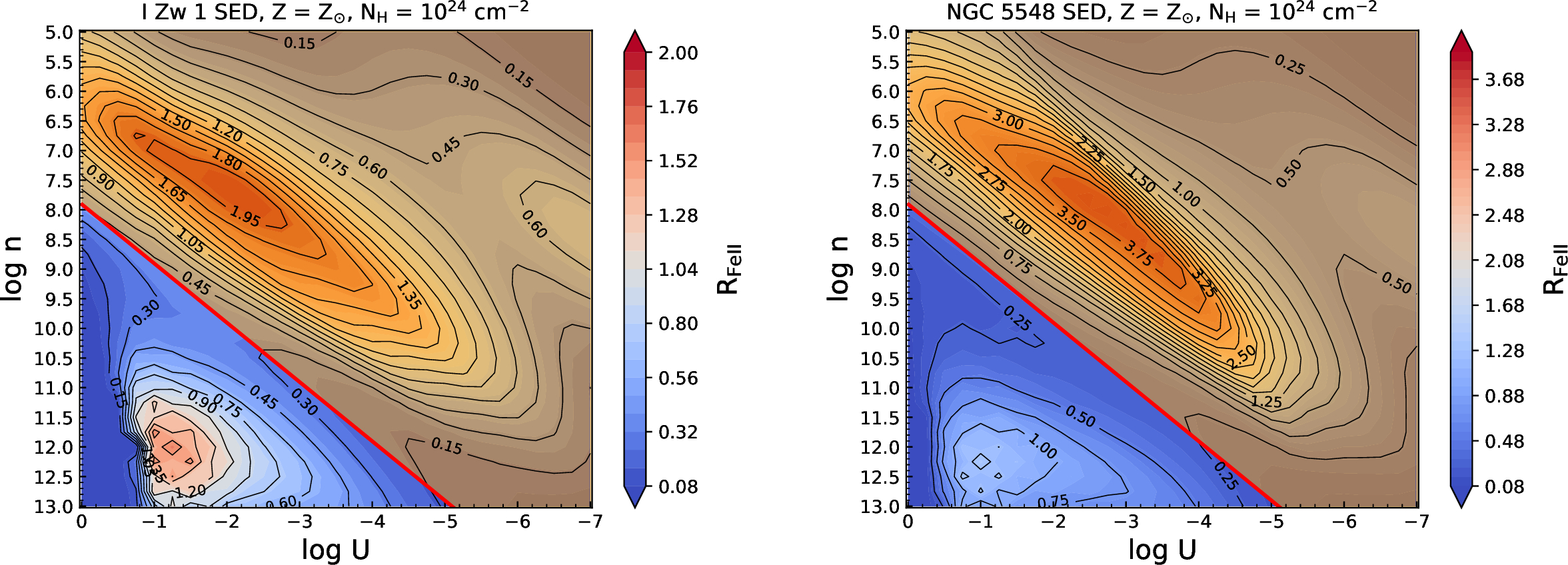
Figure 3: $\log\rm{U}-\log\rm{n_{H}}$ 2D histograms color-weighted by R${}_{\textmyfont{FeII}}$. Remaining labels and parameters shown here are identical to Figure 2.

In Figure 3, we show the $\log\rm{U}-\log\rm{n_{H}}$ parameter space with the auxiliary axis depicting the ratio R${}_{\textmyfont{FeII}}$, i.e. the EW($\rm{Fe\;II}$) to the EW(H$\beta$) for the two SEDs. We have assumed that the two emission lines are produced from a similar region in the BLR (see e.g., Barth et al., 2013; Hu et al., 2015; Panda et al., 2018; Gaskell et al., 2021b) and hence the covering factor is set to be equal for both the emission lines.

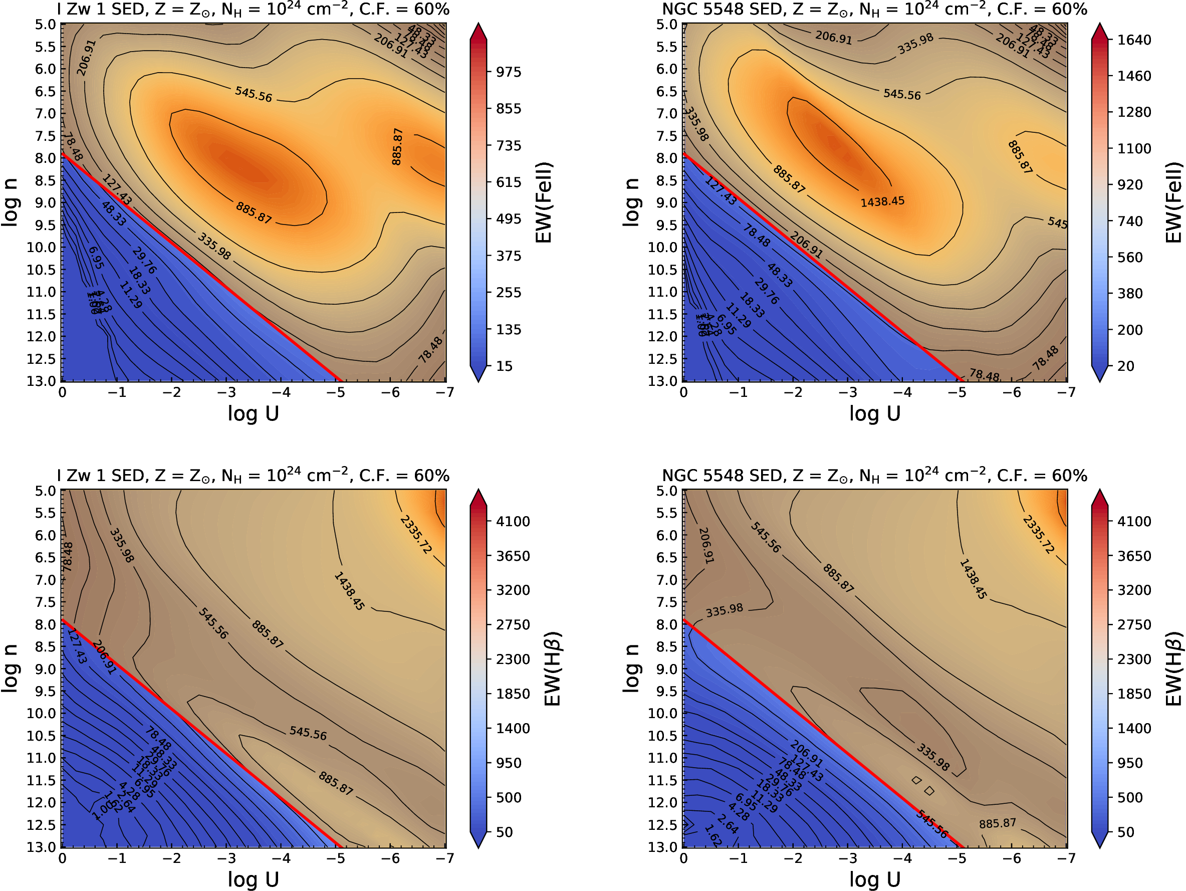
Figure 12: $\log\rm{U}-\log\rm{n_{H}}$ 2D histograms color-weighted by (top panels) equivalent width (EWs) $\rm{Fe\;II}$, and (bottom panels) EW(H$\beta$). The labels and parameters shown here are identical to Figure 2 except here we use a larger value for the covering fraction, i.e., 60%.

We also consider a case with a higher covering factor (i.e., 60%) to highlight the effect due to non-radial motions (Kollatschny and Zetzl, 2013) or changes in the accretion disk structure (Abramowicz et al., 1988; Wang et al., 2014). This higher value for the covering factor is an upper threshold as modelled in the locally optimized cloud models by Korista and Goad (2000) for NGC 5548. This is shown in Figure 12 under the same conditions as for the case with the 20% covering factor.

5.3 Comparison with reverberation-mapped estimates

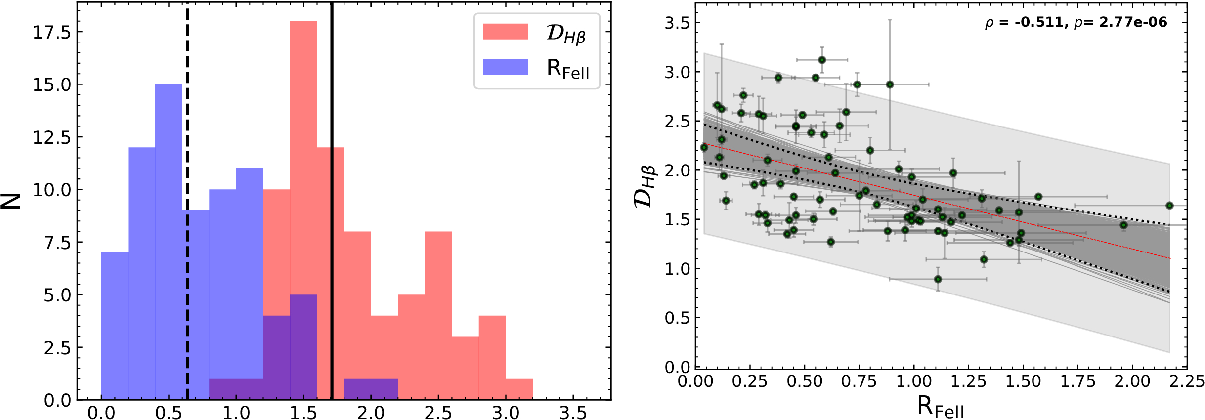
Figure 4: (Left:) Distribution of the $\mathcal{D_{\rm H\beta}}$ (in red) and R${}_{\textmyfont{FeII}}$ (in blue) for the sample from Du and Wang (2019) and as shown in Table LABEL:tab:rm-data. The median values for the two parameters are shown using the vertical lines - solid ($\mathcal{D_{\rm H\beta}}$) and dashed (R${}_{\textmyfont{FeII}}$). (Right:) Correlation between the $\mathcal{D_{\rm H\beta}}$ and R${}_{\textmyfont{FeII}}$ for this sample (see also Figure 2 in Du and Wang (2019)). The Spearman’s rank correlation coefficients ($\rho$) and the $p-$values are also reported. The ordinary least-square (OLS) fit for each panel is shown using red solid line. Black dotted lines mark the confidence intervals at 95% for the 1000 realizations (dark gray lines) of the bootstrap analysis. The corresponding prediction intervals are shown in the background using light gray color.

To make a quantitative comparison with the results from the CLOUDY simulations, we utilize the sample of reverberation-mapped AGNs from Du and Wang (2019). The sample consists of 75 AGNs for which an independent and homogeneous spectral fitting in the optical region (including the 4430–5550Å  window in the rest frame) was performed in their paper. The spectral window includes the H$\beta$ and optical $\rm{Fe\;II}$ emission blend (between 4434-4684 Å) that is necessary to estimate the ratio, R${}_{\textmyfont{FeII}}$, the bolometric luminosity using the AGN luminosity at 5100Å  and the black hole mass using the FWHM(H$\beta$) in association with the distance of the BLR from the central continuum source which is obtained from various reverberation mapping campaigns (see Section 2.1 in Du and Wang, 2019, where they list the various campaigns), and thus the Eddington ratio or its equivalent - the dimensionless accretion rate ($\mathcal{\dot{M}}$). We present the spectral and derived properties of this sample in Table LABEL:tab:rm-data, that includes the AGN luminosity at 5100Å  ($\mathrm{L_{5100}}$), the black hole mass ($M\mathrm{{}_{BH}}$), the $\mathcal{\dot{M}}$, R${}_{\textmyfont{FeII}}$ and the $\mathcal{D_{H\beta}}$, where the latter is the ratio of the FWHM(H$\beta$) to the dispersion of the H$\beta$. To estimate the $\mathcal{\dot{M}}$, the authors (e.g., Wang et al., 2013; Du et al., 2015, 2016; Du and Wang, 2019) use the following form:

$$\mathcal{\dot{M}}=20.1\left(\frac{l_{44}}{\rm{cos}\;i}\right)^{\frac{3}{2}}m_{7}^{-2}$$ (12)

where, the $l_{44}$ is the AGN luminosity at 5100Å  in the units of 10⁴⁴ erg s^-1, the $m_{7}$ is the black hole mass in the units of 10⁷ M_⊙, and $i$ is the inclination angle of the accretion disk. The estimates for the $\dot{\mathcal{M}}$ tabulated in their paper (Du and Wang, 2019) and in Table LABEL:tab:rm-data assume an average value of the cos $i$ = 0.75. Since the $\dot{\mathcal{M}}$ and Eddington ratio are equivalent, we can express the Eddington ratio ($L\mathrm{{}_{bol}}/L\mathrm{{}_{Edd}}$) as follows:

$$\frac{L_{\rm bol}}{L_{\rm Edd}}=7.455\times 10^{-18}\left(k_{\rm bol}M_{\rm BH}^{\frac{1}{3}}\mathcal{\dot{M}}^{\frac{2}{3}}\right)$$ (13)

Thus, any inferences that will be drawn based on the $\dot{\mathcal{M}}$ can be extended directly to the corresponding estimates of the Eddington ratios. We decided to use this particular sample to ensure that the sources are treated in the same manner. This removes the bias from fitting techniques employed by different groups. An independent spectral fitting incorporating newer measurements and newer sources is needed which is outside the scope of this paper.

Next, we show the distribution of the estimates for the R${}_{\textmyfont{FeII}}$ and for the $\mathcal{D_{H\beta}}$ for this sample in the left panel of Figure 4. The range of R${}_{\textmyfont{FeII}}$ values lie between [0.04, 2.17], while for the $\mathcal{D_{H\beta}}$ this range is between [0.89, 3.12]. Thus, according to the definition of the spectral sub-types in the optical plane of the main sequence (see Figure 1, also in Marziani et al., 2018; Panda et al., 2019c, 2020b), this sample is dominated by Population A sources (51/75) and covers the spectral types from A1-A4. Here A1 are the more typical, low-R${}_{\textmyfont{FeII}}$ ($\leq$ 0.5) AGNs and the A4 are the more rare, strong-$\rm{Fe\;II}$ emitters ($\geq$ 2.0). In addition, we have a considerable number of Population B sources in this sample (24/75) including the NGC 5548. We refer the readers to Table 1 in Du and Wang (2019) for the estimates for the FWHMs for the sources in the sample. In the right panel of 4, we show the strong anti-correlation between R${}_{\textmyfont{FeII}}$ and $\mathcal{D_{H\beta}}$ (see also Figure 2 in Du and Wang 2019). This figure re-iterates an already known fact, i.e., the sources with high R${}_{\textmyfont{FeII}}$ (especially $\gtrsim$ 1) also are found to have higher accretion rates and this then affects the emission line profiles - making them more Lorentzian, as opposed to the generally well-fitted Gaussian profiles that is suited for the sources with low R${}_{\textmyfont{FeII}}$ estimates (e.g. typical Population B sources). This change in the line profiles affects directly the value of the $\mathcal{D_{H\beta}}$ - for a pure Lorentzian this value tends to zero, while for a single Gaussian this value is 2$\sqrt{2\rm{ln}(2)}$ = 2.35. For a rectangular function, $\mathcal{D_{H\beta}}$ = 2$\sqrt{3}$ = 3.46 (Collin et al., 2006). We describe the analytical formulations including the $\mathcal{D_{\rm H\beta}}$ in our prescription in the Appendix A.

6 Results

6.1 Understanding the $\log\rm{U}-\log\rm{n_{H}}$ parameter space for I Zw 1 and NGC 5548

In the following sections, we describe the results from the various CLOUDY photoionization models that were made to constrain the physical parameter space in terms of the $\log\rm{U}-\log\rm{n_{H}}$ diagrams. The key here is the focus on the recovery of the EWs for the two low ionization emission lines - H$\beta$ and $\rm{Fe\;II}$, in addition to the ratio of their EWs, i.e., R${}_{\textmyfont{FeII}}$. In Figure 2, we depict the EW($\rm{Fe\;II}$) and the EW(H$\beta$) for the two sources (I Zw 1 and NGC 5548) under the assumption that the BLR in the two cases has solar composition and the covering factor is identical, i.e. 20%. Another important highlight is the separation of the dustless region from the region where dust can survive. Species like the $\rm{Fe\;II}$ get strongly depleted in the presence of dust and can be used as a tracer for the dust in the extended, intermediate-line regions that are located further away from the BLR (see e.g., Adhikari et al., 2016). As described in Section 5.1, we have made a simple assumption on the location of the dust sublimation radius that is effectively dependent only on the AGN luminosity. This uniquely sets the dust sublimation radius for each source (see Table 2). In Figure 2 (and henceforth), we have used the dust sublimation radius case assuming the luminosity-dependent $k\mathrm{{}_{bol}}$ correction that gives a slightly larger value for this radius. In the figure, the radius ($R$) is shown using a red solid line which corresponds not to the $R\mathrm{{}_{BLR}}$ but to a radius that is much larger than $R\mathrm{{}_{BLR}}$. The values for this larger $R$ in terms of $\rm{U}$$\rm{n_{H}}$ are very similar for the two sources as the differences in their luminosities and radial extensions almost balances out - (a) for NGC 5548, 7.9030 (for the luminosity-dependent $k\mathrm{{}_{bol}}$); (b) for I Zw 1, 7.9040 (for the luminosity-dependent $k\mathrm{{}_{bol}}$). The corresponding R${}_{\textmyfont{FeII}}$ estimates for the two cases (see Figure 3) also have similar demarcations.

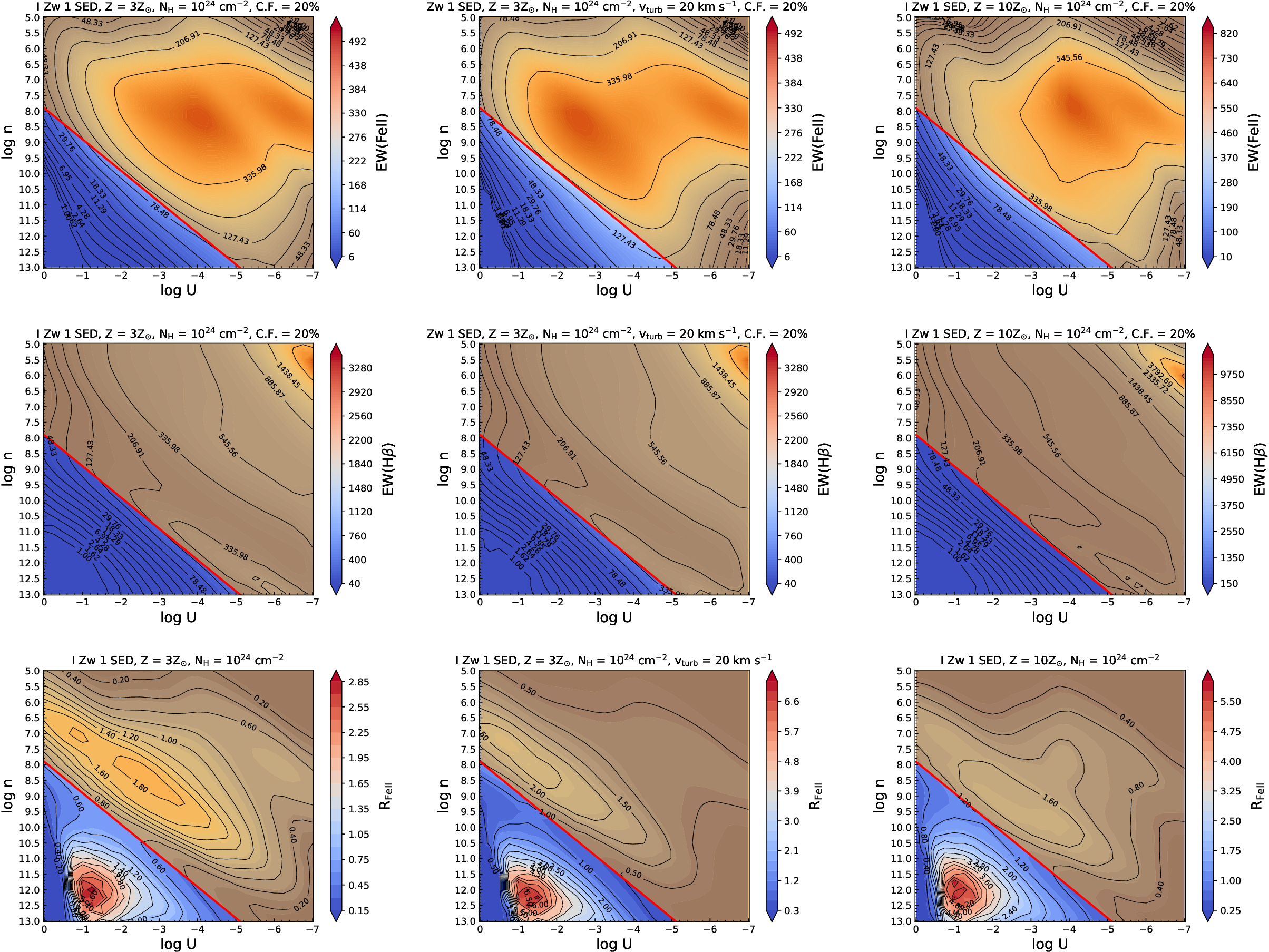
Figure 5: $\log\rm{U}-\log\rm{n_{H}}$ 2D histograms color-weighted by (top panels) equivalent width (EWs) $\rm{Fe\;II}$, (middle panels) EW(H$\beta$), and (bottom panels) R${}_{\textmyfont{FeII}}$. The labels and parameters shown here are identical to Figure 2. The panels depict the models considered for a BLR metallicity of 3Z_⊙ (left panels), then for a metallicity of 3Z_⊙ with additional microturbulence of 20  km s^-1 (middle panels), and, for a metallicity of 10Z_⊙ (right panels).

6.2 Comparing the reverberation-mapped sources with the CLOUDY models

Another way of looking at this scenario is by comparing the product of the $\rm{U}$ and $\rm{n_{H}}$ directly versus the R${}_{\textmyfont{FeII}}$. This is already shown from the estimates tabulated in our Table 1 for the two sources. But, as there are the various considerations for the $k\mathrm{{}_{bol}}$ and the $R\mathrm{{}_{H\beta}-L_{5100}}$ relations, the values obtained for the photoionization radius estimator, i.e., the product $\rm{U}$$\rm{n_{H}}$, varies, albeit slightly. In this section, we organize the $\log\rm{U}-\log\rm{n_{H}}$ parameter space from each model and compare the relevance of these results to the reverberation-mapped sources with spectral coverage that includes the R${}_{\textmyfont{FeII}}$ measurements. We intend to assess the changes in the SED of the two prototypical sources considered in work to see if they account for the R${}_{\textmyfont{FeII}}$ estimates reported from spectral fitting. We highlight the salient differences between the two cases, and how our analytical prescriptions reported in Section 4 perform against the numerical estimates from CLOUDY.

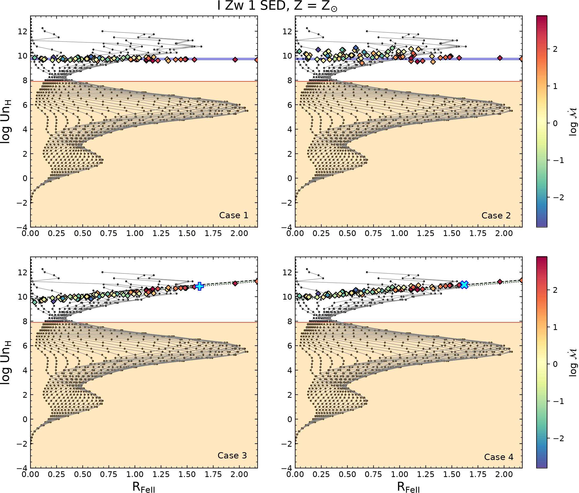
Figure 6: Grid composed of the family of distributions for the $\rm{U}$$\rm{n_{H}}$ (in log-scale) as a function of the R${}_{\textmyfont{FeII}}$ (gray lines with black dots) from one of our CLOUDY simulations - I Zw 1 SED, $N_{\rm{H}}$ = $10^{24}$ cm^-2, and, at solar composition. The shaded region in orange depicts the region within the dust and the solid red line marks the location of the dust sublimation radius as per Table 2. The sample of 75 reverberation-mapped sources (see Table LABEL:tab:rm-data) are shown for the corresponding cases of $\rm{U}$$\rm{n_{H}}$ as per the four analytical forms shown in Table 1. These sources are color-coded with their corresponding $\dot{\mathcal{M}}$ estimates. The location of the source I Zw 1 is shown using a blue cross for the lower panels where there is an explicit dependence on the R${}_{\textmyfont{FeII}}$.

In Figure 6, we show the grid from one of our CLOUDY simulations (I Zw 1 SED, $N_{\rm{H}}$ = $10^{24}$ cm^-2, and, at solar composition). The grid is composed of the family of distributions for the $\rm{U}$$\rm{n_{H}}$ (in log-scale) as a function of the R${}_{\textmyfont{FeII}}$. These are identical to what we show in the left panel of Figure 3 just represented differently. The shaded region in orange depicts the region within the dust and the solid red line marks the location of the dust sublimation radius as per Table 2. The location of the dust sublimation radius is neatly poised at one of the minima for the R${}_{\textmyfont{FeII}}$.

Preparing broad-band SEDs for the diverse population of AGNs is not easy, especially to get contemporaneous spectral or photometric data over a wide range of energies. Having SEDs that can be representative of the sub-populations, e.g., Population A and Population B, is quite useful. This was our intention from this work. To test the validity of our models on the observational estimates for sources with spectral coverage and reverberation mapping, we overlay the 75 sources from Table LABEL:tab:rm-data on these maps. These sources are colour-coded as a function of the dimensionless accretion rate ($\dot{\mathcal{M}}$). For each of the four panels, we evaluate the $\rm{U}$$\rm{n_{H}}$ for each source using the four relations as shown in the Table 1, i.e., accounting for (a) the standard $R\mathrm{{}_{H\beta}-L_{5100}}$ relation from Bentz et al. (2013) with fixed $k\mathrm{{}_{bol}}$ (Case 1) and with luminosity-dependent $k\mathrm{{}_{bol}}$ (Case 2); and (b) the R${}_{\textmyfont{FeII}}$-dependent $R\mathrm{{}_{H\beta}-L_{5100}}$ relation from Du and Wang (2019) with fixed $k\mathrm{{}_{bol}}$ (Case 3) and with luminosity-dependent $k\mathrm{{}_{bol}}$ (Case 4). For the first two cases (upper panels), we show the $\rm{U}$$\rm{n_{H}}$ for I Zw 1 using the $\mathrm{L_{5100}}$ as also reported in Table 1. These are shown using the two solid blue lines on the upper panels. As we can notice, the location of the sources on this plane is affected due to the change of the $k\mathrm{{}_{bol}}$ - a larger scatter in the $\rm{U}$$\rm{n_{H}}$ is seen especially for sources that have relatively low R${}_{\textmyfont{FeII}}$ and low to mid $\dot{\mathcal{M}}$. For the latter cases (lower panels), we show the $\rm{U}$$\rm{n_{H}}$ for I Zw 1 which is now dependent on the $\mathrm{L_{5100}}$ and R${}_{\textmyfont{FeII}}$, and hence, changes with the change in the R${}_{\textmyfont{FeII}}$. These are shown using the dashed (fixed $k\mathrm{{}_{bol}}$ case) and dotted (luminosity-dependent $k\mathrm{{}_{bol}}$) black lines on the panels. The location of I Zw 1 is shown using the blue plus and a blue cross symbol, respectively, in these two panels. The scatter in these panels is lower compared to Case 2 (upper right panel). The I Zw 1 SED under the solar composition can incorporate a large fraction of the sources in the sample, although as expected the observed R${}_{\textmyfont{FeII}}$ estimates for I Zw 1 and two other sources (SDSS J101000 and IRAS 04416+1215) is higher than predicted from these base models.

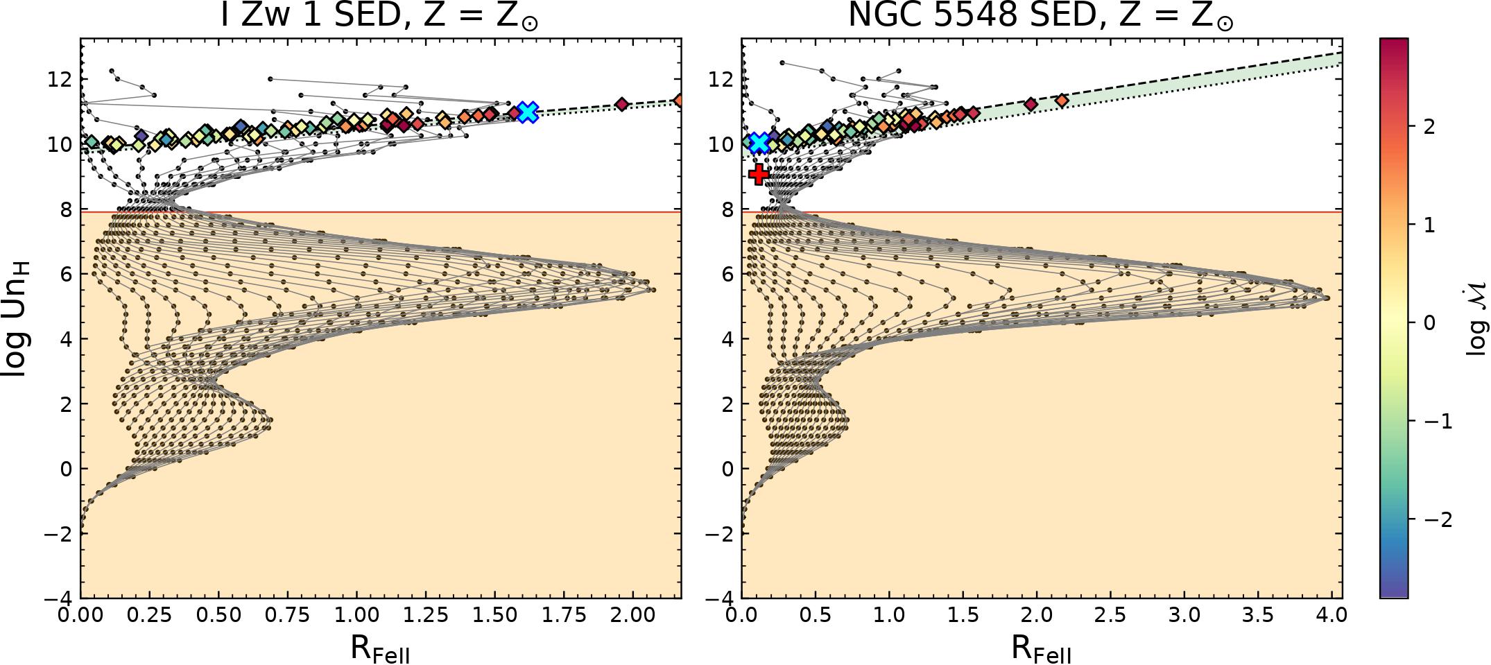
Figure 7: Similar to the last panel (Case 4) in Figure 6. Here, we compare the solar composition model for the two sources - I Zw 1 and NGC 5548. The location of the respective sources are marked using a blue cross in the corresponding panels. The red plus symbol on the right panel marks the position of the value obtained for $\rm{U}$$\rm{n_{H}}$ using the filtering of EWs (see Section 6.3).

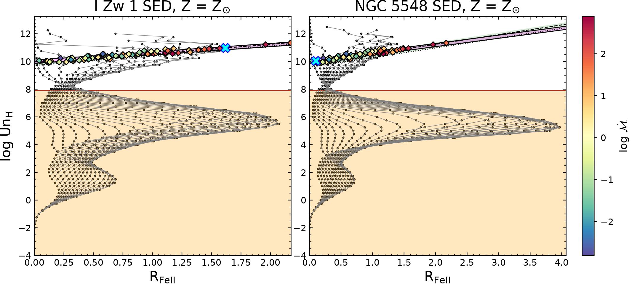
Figure 11: Similar to Figure 7 but with the inclusion of the $\mathcal{D_{\rm H\beta}}$ in the analytical prescription. The panels include the full range of the $\mathcal{D_{\rm H\beta}}$ as per min-max range from the histogram shown in Figure 4. The $\rm{U}$$\rm{n_{H}}$ estimates for the observed sample is based on the luminosity-dependent $k\mathrm{{}_{bol}}$ and R${}_{\textmyfont{FeII}}$-based $R\mathrm{{}_{H\beta}-L_{5100}}$ relation as shown in Table 3. The blue cross in each panel shows the location of the respective sources from the estimates tabulated in the last row of Table 3.

For completeness, we also show a comparison between the two SED cases at solar composition with the observed sample side-by-side in Figure 7. The left panel is identical to Case 4 already shown in Figure 6. The right panel shows the case with the $\rm{U}$$\rm{n_{H}}$ grid extracted from our CLOUDY simulations but for the NGC 5548 SED. Like in the bottom panels of Figure 6, we show the $\rm{U}$$\rm{n_{H}}$ from the analytical relations for the two panels dependent on the $\mathrm{L_{5100}}$ and R${}_{\textmyfont{FeII}}$ (shown using the dashed (fixed $k\mathrm{{}_{bol}}$ case) and dotted (luminosity-dependent $k\mathrm{{}_{bol}}$) black lines on the panels). We also locate the sources in the corresponding panels using a blue cross symbol. We can notice that the NGC 5548 sits among the lowest R${}_{\textmyfont{FeII}}$ sources. It agrees well in all of the four cases shown earlier in Figure 6 and hence is rather unaffected by the inclusion/exclusion of the fixed/variable $k\mathrm{{}_{bol}}$ or the change in the $R\mathrm{{}_{H\beta}-L_{5100}}$ relation used to infer the $\rm{U}$$\rm{n_{H}}$. Right away we notice that the NGC 5548 case predictions encompass a lower fraction of the sources than I Zw 1 case, especially those with reportedly high R${}_{\textmyfont{FeII}}$ values. The strip showing the $\rm{U}$$\rm{n_{H}}$ from the Case 3 and Case 4 is thicker in the NGC 5548 that is due to the effect of luminosity (see Table 1 with the $R\mathrm{{}_{H\beta}-L_{5100}}$ relation cases with R${}_{\textmyfont{FeII}}$-dependence). The location of the observed sources is the same in these two panels, but the extent of the overall R${}_{\textmyfont{FeII}}$ predicted with the NGC 5548 case from the models is higher - the dominant peak is located well within the dusty region. Thus, the I Zw 1 case predicts higher R${}_{\textmyfont{FeII}}$ in the dustless region, as expected from the observed values. We also mark a red plus symbol on the right panel of this figure which marks the position of the value obtained for $\rm{U}$$\rm{n_{H}}$ after careful filtering of the possible pairs of solutions by comparing the EWs of both the $\rm{Fe\;II}$ and the H$\beta$ belonging to the non-dusty part of the BLR. We expand more on this issue in the next section (see Section 6.3). We also make a comparative analysis between the two cases including the $\mathcal{D_{\rm H\beta}}$ parameterization within our analytical formalism (see Figure 11).

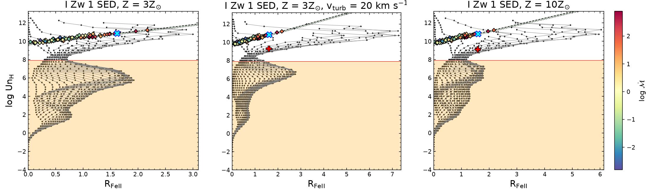
Figure 8: Similar to the last panel (Case 4) in Figure 6. Here, we compare I Zw 1 models at 3Z_⊙, at 3Z_⊙ with an additional microturbulent velocity 20  km s^-1, and at 10Z_⊙. The location of the respective sources are marked using a blue cross in the corresponding panels. The red plus symbol on the right panel marks the position of the value obtained for $\rm{U}$$\rm{n_{H}}$ using the filtering of EWs (see Section 6.3).

Subsequently, following the results that were obtained earlier with the I Zw 1 necessitating an increased metal content (and turbulent motions) within the BLR (see Section 6.1), we show the grids of $\rm{U}$$\rm{n_{H}}$ for each of the three cases - at 3Z_⊙, at 3Z_⊙ with 20  km s^-1 microturbulence, and finally, the case with the 10Z_⊙. Figure 8 shows these three cases. The dominant peak in these cases shift to the region that corresponds to the dustless BLR (i.e., with $\rm{U}$$\rm{n_{H}}$ $\gtrsim$ 8.0). Already in just the 3Z_⊙ case (left panel in Figure 8), all the observed estimates are well within the grid lines extracted from the models. But as we have emphasized before, this needs to be supplemented with the EWs recovered for the sources using the models. With these plots, we wanted to show that the effect of the SED with the added contribution of the metal content and microturbulence can significantly affect the recovery of the R${}_{\textmyfont{FeII}}$ and that SEDs for prototypical sources (like NGC 5548 and I Zw 1) can be used to infer properties of sources alike. Similar to the previous figure (the right panel with NGC 5548), we show the value obtained for $\rm{U}$$\rm{n_{H}}$ after the EW-filtering using a red plus symbol.

6.3 Bringing it all together - filtering the optimal ($\rm{U}$,$\rm{n_{H}}$) and EWs

Now focusing our attention to the non-dusty part of the BLR, we would like to compare the estimates for the EWs for these two lines obtained from the observations and extract the optimal pairs of solution(s) for the $\rm{U}$ and $\rm{n_{H}}$. We use the estimates that were quoted by Du and Wang (2019) for (a) NGC 5548: EW($\rm{Fe\;II}$) = 11.8$\pm$1.4, EW(H$\beta$) = 117.8$\pm$27.3 (this gives an R${}_{\textmyfont{FeII}}$=0.1$\pm$0.02); and from Marziani et al. (2021, submitted) for (b) I Zw 1: EW($\rm{Fe\;II}$) = 72.86$\pm$15.04, EW(H$\beta$) = 45.0$\pm$9.42 (this gives an R${}_{\textmyfont{FeII}}$=1.619$\pm$0.06).

We can see from the right panels in Figure 2 which is depicting the case of NGC 5548, that we are successful in recovering these estimates for the EWs for the two species. Although, for the case of I Zw 1, while we are almost able to get the match for the EW(H$\beta$), the EW($\rm{Fe\;II}$) is considerably underestimated. The higher values for the EWs are seen for the regions which are shrouded in the dust where both the ionization parameter and BLR densities are quite low from the viewpoint of the BLR emission (see e.g., Negrete et al., 2012; Marziani et al., 2018; Panda et al., 2018; Śniegowska et al., 2021). There is a slight increase when we consider a higher covering factor (60%, see Figure 12) but still a deficit of $\sim$10-20Å  is found for this case. Next, we proceed on to testing with higher metal content in the BLR. In Figure 5, we show the results for the consideration of two cases of super-solar metallicity - 3Z_⊙ (left panels) and 10Z_⊙ (right panels). We have again assumed the 20% covering factor to estimate the EWs. As we can notice, the case with 3Z_⊙ is still unable to recover the EW($\rm{Fe\;II}$) as suggested from the observations. But, when we go to an even higher metal content (10Z_⊙), we are eventually successful. On the other hand, the BLR cloud can be locally turbulent (Baldwin et al., 2004; Bruhweiler and Verner, 2008; Shields et al., 2010; Kollatschny and Zetzl, 2013) and it has been shown to substantially affect the $\rm{Fe\;II}$ spectrum by facilitating continuum and line-line fluorescence (see e.g., Shields et al., 2010; Panda et al., 2018, 2019a; Sarkar et al., 2021). We consider a microturbulence value of 20  km s^-1 suggested by our previous works (Panda et al., 2018, 2019a) and complement it with the case at 3Z_⊙. The middle panels in Figure 5 show the results from this model. We notice that this case can reproduce the EW($\rm{Fe\;II}$) as well, in addition to the successful recovery of the EW(H$\beta$) and hence, the R${}_{\textmyfont{FeII}}$. We would like to emphasize that the suggested solutions in terms of $\rm{U}$ and $\rm{n_{H}}$ are not the ones that show the maximum R${}_{\textmyfont{FeII}}$, rather the ones where both the EWs and the R${}_{\textmyfont{FeII}}$ are in agreement with the observations. Thus, a small microturbulence can affect the recovery of the $\rm{Fe\;II}$ and hence the R${}_{\textmyfont{FeII}}$ and the model thus don’t necessitate the exceptionally high metal content. For I Zw 1, we find that the best agreement is obtained with a metal content that is slightly super-solar (Z$\gtrsim$3Z_⊙) with the inclusion of turbulent motions within the BLR cloud (see also Panda, 2021b, for an overview on the effect of microturbulence in I Zw 1).

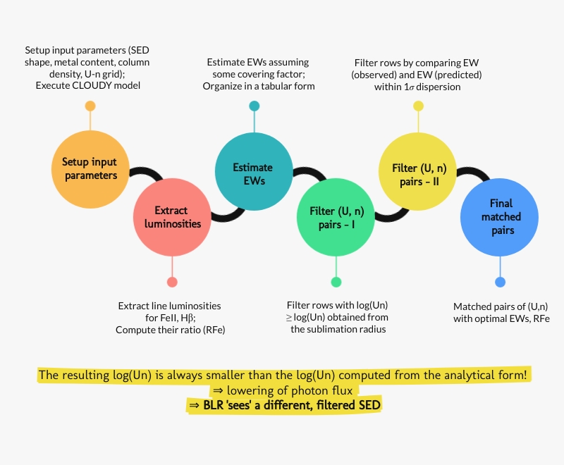
Figure 9: Flowchart depicting the steps taken in the filtering process - starting from the preparation of the input setup till procuring the matched pairs of ($\rm{U}$,$\rm{n_{H}}$) for each model described in this paper.

In order to finalize the pairs of ($\rm{U}$,$\rm{n_{H}}$) we illustrate our filtering process in Figure 9. This outlines how we arrive at the solutions for these physical parameters in the non-dusty part of the BLR that best represent the conditions in the H$\beta$ and $\rm{Fe\;II}$ line emitting region. We start with making a first filtering by accounting for the subset of the $\log\rm{U}-\log\rm{n_{H}}$ where their product is at or larger than the $\rm{U}$$\rm{n_{H}}$ estimated using the dust sublimation radius for the corresponding cases, e.g. for I Zw 1 considering the luminosity-dependent $k\mathrm{{}_{bol}}$, we have the $\rm{U}$$\rm{n_{H}}$ (in log-scale) = 7.9040. Next, we filter from the remaining set of those that agree in their EWs (simultaneously for $\rm{Fe\;II}$ and H$\beta$) predicted by CLOUDY to their observed values within 1-$\sigma$ dispersion (of the observed value). The final remaining solutions are plotted in Figure 10 for the cases where the agreement is found on all counts. We see that as we expected, for I Zw 1, the cases with 3Z_⊙ with a small microturbulent velocity (v_turb = 20  km s^-1), and the case with 10Z_⊙, are well-suited. While for NGC 5548, the BLR cloud with solar abundance is sufficient. Although in this case we recover only one pair of solution (see the triangle marked in Figure 10) where the predicted density is quite low and the ionization parameter is significantly higher. The single cloud assumption that we make here to perform the CLOUDY modelling needs to be revisited and compared against its counterpart, e.g. the locally optimized cloud model (LOC, Baldwin et al., 1995; Korista and Goad, 2000), wherein the setup assumes a system of clouds with distribution in density and location from the central source. The LOC model has been shown to agree better particularly in the case of NGC 5548. A subsequent work is under progress that deals with this exact issue. While, in the case of I Zw 1, as also discussed in Panda (2021b), the increase in the accretion rate may puff up the very inner regions of the accretion disk leading to the BLR receiving a filtered SED, one that is significantly different from the SED that is observed by a distant observer, and with much less ionizing photons. This may further lead to the inward shift in the location of the clouds due to reduced radiation pressure in the BLR region. This may lead to cloud coagulation one that is well-described by a single cloud model.

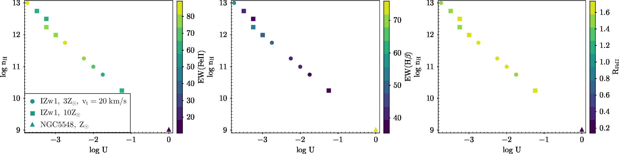
Figure 10: The $\log\rm{U}-\log\rm{n_{H}}$ parameter space as a function of: (a) EW($\rm{Fe\;II}$), (b) EW(H$\beta$), and, (c) R${}_{\textmyfont{FeII}}$. These mark the final filtered solutions adopting the steps shown in Figure 9. The three successful cases (two for I Zw 1, and, one for NGC 5548) are shown using respective symbols.

In Figure 10, we can get the exact values of the product of the $\rm{U}$$\rm{n_{H}}$ which is in the range 9-9.25 for I Zw 1, and 9 for NGC 5548. Now coming back to the red plus symbol that were marked in the panels of Figures 7 and 8, we see that the solution obtained from our analytical formulation (see Table 1) and the solution obtained from this filtering process differ by almost 2 dex, i.e., for the luminosity-dependent $k\mathrm{{}_{bol}}$ case with R${}_{\textmyfont{FeII}}$-based $R\mathrm{{}_{H\beta}-L_{5100}}$ relation, we get a $\rm{U}$$\rm{n_{H}}$ = 10.939. Taking a ratio of the two $\rm{U}$$\rm{n_{H}}$ from these different formalisms, we get a value between 1-2%. This is what is the fraction of the actual number of ionizing photon flux that is received at the BLR that leads to the line-formation and emission of the H$\beta$ and $\rm{Fe\;II}$ in I Zw 1. This is exactly what we realized in our previous work (Panda, 2021b) - that the BLR “sees” a different, filtered SED with only a very small fraction ($\sim$1%) that leads to the line emission in the low-ionization emitting region of the BLR. With a rigorous filtering approach, we have confirmed this hypothesis in this work. Similarly for NGC 5548, for the luminosity-dependent $k\mathrm{{}_{bol}}$ case with R${}_{\textmyfont{FeII}}$-based $R\mathrm{{}_{H\beta}-L_{5100}}$ relation, we get a $\rm{U}$$\rm{n_{H}}$ = 10.008. The fraction of the photon flux recovered is $\sim$10%. We note that these estimates for the fraction of ionizing continuum received by the BLR are obtained for a pre-assumed value of $\chi$ = 0.5 (where $\chi$ is the ratio of L_ion to the $\mathrm{L_{bol}}$ predicted by CLOUDY for each input SED). Changing the $\chi$ to a value consistent for the I Zw 1 SED, i.e., 0.12, we get the actual ionizing continuum received by the BLR to be between $\sim$5-10%. For NGC 5548, this fraction is much higher ($\chi$=0.82). Thus, the actual ionizing continuum in this case received by the BLR is still $\sim$10%.

Hence, through this analysis we realize the importance of the actual ionizing luminosity, in addition to the $\mathrm{L_{5100}}$ and R${}_{\textmyfont{FeII}}$ estimated from their respective spectra, that recovers the pairs of ionization parameter and local BLR density, one that is representative of the properties of the low-ionization line emitting BLR. This ionizing luminosity is estimated with the knowledge of the exact shape of the SED for the corresponding source. In view of a series of work (Negrete et al., 2013; Marziani and Sulentic, 2014; Panda et al., 2019c; Ferland et al., 2020; Marziani et al., 2021) that have highlighted the importance of having the SED shape properly modelled, subsequent studies accounting for the proper SED fitting of other sources will strengthen the framework presented in this paper.

7 Discussions

As briefly mentioned in the earlier sections, the assumption of the covering factor is perhaps the only weakness in the current model. This value is important to estimate the EW for the respective emission lines. Broad-band SED modelling that includes the torus properties can allow constraining this parameter, either through the study of individual sources (e.g., Mor et al., 2009) or from large surveys utilizing the optical and infrared fluxes as a proxy for the covering factors (e.g., Roseboom et al., 2013). Another effective way would be to estimate this parameter using dynamical modelling of the BLR (e.g., Pancoast et al., 2014; Li et al., 2016).

Next, is the issue of constraining the SED through robust modelling and high-quality contemporaneous spectroscopic measurements across the optical, ultraviolet and X-ray energies as has been done for NGC 5548 and a few other sources (see e.g., Kubota and Done, 2019; Ferland et al., 2020). We need to test the viewing angle-dependent SEDs (e.g., Wang et al., 2014) and compare the modelled predictions to infer physical conditions of the BLR more appropriately.

The location of the dust sublimation radius affects the results obtained in this work. Our assumptions are also supported by Suganuma et al. (2006) which found lags of hot dust emission in AGNs to be $\sim$3.5 times the lag of H$\beta$ (see their Figure 32a). They thus confirm that region with species like O^∘, Mg⁺, Ca⁺ and Fe⁺ lies just inside the hot dust, and in the very outermost part of the BLR. This inference is also validated from our results obtained in this work and earlier in Panda et al. (2020a); Panda (2021b).

Another important aspect of the work is the reliability of the spectral fitting techniques and the inference of the R${}_{\textmyfont{FeII}}$. Tests with refined templates (e.g., Park et al., 2021; Marziani et al., 2021) needs to made to constrain the R${}_{\textmyfont{FeII}}$ better for the available sources with high S/N spectroscopy. These then need to be compared with better photoionization models that include $\rm{Fe\;II}$ databases including higher number of transitions (e.g., Sarkar et al., 2021). Our results have shown that whatever is causing H$\beta$ to vary is also similarly causing $\rm{Fe\;II}$ to vary as well. One can also see in Figure 5 of Gaskell et al. 2021b that both H$\beta$ and $\rm{Fe\;II}$ track the broad features of the continuum variability suggesting similar origins with subtle differences. Better $\rm{Fe\;II}$-based reverberation mapping estimates are needed to constrain the location of the $\rm{Fe\;II}$-emitting region in the BLR. This is located further away from the central engine compared to the H$\beta$ - by a factor $\sim$2 (Gaskell et al., 2021b, 2007) that is confirmed by the high-cadence reverberation mapping results from Barth et al. (2013); Hu et al. (2015). Another interesting aspect is the “breathing” mode that has been seen especially in the Balmer lines (Korista and Goad, 2004; Barth et al., 2015; Runco et al., 2016; Gaskell et al., 2021a). The variability pattern in the Balmer lines, also studied in the MgII (see e.g., Guo et al., 2020), indicate that the location of the onset of the BLR ($R\mathrm{{}_{BLR}}$) can change due to the increase/decrease in the intrinsic luminosity of the source. In order to study this effect and incorporate into our formalism, we need to systematically prepare broad-band SEDs that are representative of such varied epochs in a source. This requires a wide coverage in wavelength, spanning from the optical to X-rays, in addition to AGN continuum light curves. A combination of the two can allow us to test the implication of the breathing mode in terms of the systematic shift in the location of the source in terms of the $\log\rm{U}-\log\rm{n_{H}}$.

On the other hand, the $R\mathrm{{}_{H\beta}-L_{5100}}$ relation needs to be tested with the inclusion of more reverberation mapped sources spanning the extent of the continuum luminosity. Better proxies of the accretion rate (or $L\mathrm{{}_{bol}}/L\mathrm{{}_{Edd}}$) are now available, e.g., the near-infrared Ca ii triplet emitting at $\lambda$8498Å, $\lambda$8542Å  and $\lambda$8662Å(Panda et al., 2020a; Martínez-Aldama et al., 2021a, b). The prospects for this channel will only get better with the upcoming James Webb Space Telescope and other ground-based observatories, e.g., the Maunakea Spectroscopic Explorer (Marshall et al., 2019) and, the European Extremely Large Telescope (Evans et al., 2015).

Finally, GRAVITY is just starting to resolve the outer BLR for nearby sources, e.g., 3C 273 (GRAVITY Collaboration et al., 2018) and IRAS 09149-6206 (Gravity Collaboration et al., 2020) using fantastic interferometric capabilities. And with the upcoming upgrade leading to the GRAVITY+, this will only get better providing us with a spectacular angular resolution that will enable us to pinpoint the location of the BLR in nearby AGNs. Yet, currently, the combination of reverberation mapping and photoionization-based results remains the only credible way to infer the location and physical conditions of these media.

8 Conclusions

Through this study, we have:

• Tested the variation in the low-ionization emitting regions of the BLR, by accounting for the changes in the shape of the ionizing continuum (the SED) and the location of the BLR from the central ionizing source (or $R\mathrm{{}_{BLR}}$) from the reverberation mapping, in the Eigenvector-1 context. We compare the SEDs for a prototypical Population A and Population B source, I Zw 1 and NGC 5548, respectively in our photoionization modelling using CLOUDY.

• Brought together our knowledge of the BLR $R\mathrm{{}_{H\beta}-L_{5100}}$ relations (Bentz et al., 2013; Du and Wang, 2019) and the photoionization theory into a unified picture. We highlight the importance of the estimation of the bolometric luminosity that is either (a) scaled-up using the monochromatic luminosity at, e.g., 5100 Å , with a fixed factor derived using composite SEDs for Type-1 quasars by combining mid-infrared and optical colours (Richards et al., 2006); or (b) uses a luminosity-dependent factor derived using theoretical calculations of optically thick, geometrically thin accretion disks, and observed X-ray properties of AGNs (Netzer, 2019). We incorporate the two widely used $R\mathrm{{}_{H\beta}-L_{5100}}$ relations - the classical Bentz et al. (2013) relation and the R${}_{\textmyfont{FeII}}$-dependent $R\mathrm{{}_{H\beta}-L_{5100}}$ from Du and Wang (2019) in this approach and compare their behaviour with the photoionization models. Additionally, we test the effect of the inclusion of the $\mathcal{D_{H\beta}}$ in our prescription.

• Tested the dependence of the location of the optical $\rm{Fe\;II}$ and H$\beta$ emitting region within the dustless BLR for various cloud parameters, namely, the metal content and turbulence within the BLR cloud. We find that for the case of NGC 5548, the solar composition is optimal in recovering the flux ratios. While, for the I Zw 1 case, the successful models require a BLR composition at least 3Z_⊙ with an added effect from turbulence within the cloud. This leads to the enhanced $\rm{Fe\;II}$ emission that then matches the observed estimates.

• Estimated the EWs for the H$\beta$ and $\rm{Fe\;II}$ from our photoionization models accounting for covering factors that are verified from previous studies (Korista and Goad, 2000; Baldwin et al., 2004; Panda, 2021b). We identify pair(s) of solutions for the ionization parameter ($\rm{U}$) and local BLR density ($\rm{n_{H}}$) that agree with the observed line EWs for the low-ionization emitting regions of the dustless BLR. This result highlights the shift in the overall $\rm{U}$$\rm{n_{H}}$ recovered from our analysis towards lower values (by up to 2 dex) compared to the $\rm{U}$$\rm{n_{H}}$ values estimates from the photoionization theory. This confirms our hypothesis that the BLR “sees” a different, filtered SED with only a very small fraction ($\sim$1-10%) that leads to the line emission in the dustless, low-ionization emitting region of the BLR.

Conflict of Interest Statement

The author declares that the research was conducted in the absence of any commercial or financial relationships that could be construed as a potential conflict of interest.

Author Contributions

The idea, analysis and writing of the manuscript has been carried by SP.

Funding

The project was partially supported by the Polish Funding Agency National Science Centre, project 2017/26/A/ST9/00756 (MAESTRO 9) and by Conselho Nacional de Desenvolvimento Científico e Tecnológico (CNPq) Fellowship (164753/2020-6).

Data Availability Statement

The setup and the results from the photoionization simulations using CLOUDY can be made available upon request to the author.

Appendix A Including the $\mathcal{D_{\rm H\beta}}$ parameter

Another interesting bi-variate relation is found between the $L\mathrm{{}_{bol}}/L\mathrm{{}_{Edd}}$ which is a function of (a) the shape of the broad-line profile ($\mathcal{D}_{H\beta}=FWHM/\sigma_{H\beta}$), and (b) the parameter R${}_{\textmyfont{FeII}}$. The $\mathcal{D}_{\rm H\beta}$ is better known as the line-width ratio (see e.g., Kollatschny and Zetzl, 2013), i.e. the ratio between the full-width at half maximum (FWHM) of the emission line (here, H$\beta$) and the corresponding dispersion in the H$\beta$ line ($\sigma_{\rm H\beta}$). In Du et al. (2016), the authors provided a novel relation that is stated as the fundamental relation for the BLR and has the form,

$$\log\lambda_{\rm{Edd}}=\alpha^{\prime}+\beta\mathcal{D}_{H\beta}+\gamma R_{\mathrm{\textmyfont{Fe II}}}$$ (14)

The values taken by the coefficients are: $\alpha^{\prime}$ = 0.31 $\pm$ 0.30, $\beta$ = -0.82 $\pm$ 0.11, and $\gamma$ = 0.80 $\pm$ 0.20.

The monochromatic luminosity at 5100Å ($\mathrm{L_{5100}}$) can be re-written using the black hole mass ($M\mathrm{{}_{BH}}$) and the Eddington ratio, i.e., $\lambda_{\rm{Edd}}$ = $L\mathrm{{}_{bol}}/L\mathrm{{}_{Edd}}$. Again, we have two versions with the inclusion of the bolometric correction factor. Assuming the fixed $k\mathrm{{}_{bol}}$ = 9.26 (Richards et al., 2006), we have

$$\log(\rm{L_{5100}})=\log\left(\frac{\rm{L_{bol}}}{9.26}\right)=\log\left(\frac{\rm{\lambda_{Edd}L_{Edd}}}{9.26}\right)=\log(\rm{\lambda_{Edd}})+\log(\rm{M_{BH}})+37.13375956$$ (15)

While on the other hand assuming the variable $k\mathrm{{}_{bol}}$ (Netzer, 2019), we have

$$\log(\rm{L_{5100}})=\log\left(\frac{\rm{L_{bol}}}{k_{bol}}\right)=1.25\left[\log(\rm{\lambda_{Edd}})+\log(\rm{M_{BH}})\right]+35.12288819$$ (16)

Incorporating this BLR fundamental plane relation in our previously obtained analytical relations with $\log\rm{Un_{H}}$ we get the following relations:

Applying Equation 14 in Equation 6 with Equation 15, we have

$$\boxed{\log(Un_{H})=9.694-0.084\log\left(\frac{\rm{M_{BH}}}{10^{8}\;\rm{M_{\odot}}}\right)+0.069\mathcal{D_{\rm H\beta}}-0.067\rm{R_{FeII}}}$$ (17)

Applying Equation 14 in Equation 7 with Equation 16, we have

$$\boxed{\log(Un_{H})=9.621-0.355\log\left(\frac{\rm{M_{BH}}}{10^{8}\;\rm{M_{\odot}}}\right)+0.291\mathcal{D_{\rm H\beta}}-0.284\rm{R_{FeII}}}$$ (18)

Applying Equation 14 in Equation 9 with Equation 15, we have

$$\boxed{\log(Un_{H})=9.769+0.1\log\left(\frac{\rm{M_{BH}}}{10^{8}\;\rm{M_{\odot}}}\right)-0.082\mathcal{D_{\rm H\beta}}+0.78\rm{R_{FeII}}}$$ (19)

Applying Equation 14 in Equation 10 with Equation 16, we have

$$\boxed{\log(Un_{H})=9.709-0.125\log\left(\frac{\rm{M_{BH}}}{10^{8}\;\rm{M_{\odot}}}\right)+0.103\mathcal{D_{\rm H\beta}}+0.6\rm{R_{FeII}}}$$ (20)

The estimates from the above analytical relations are summarised in Table 3. Similar to Table 1, we report the estimates for all the cases accounting for the appropriate $\chi$ values for the two sources in the last two columns in Table 3.

Table 3: Estimates for log(Un_H) for the various relations considered in this paper including the $\mathcal{D_{\rm H\beta}}$ parameter

Radius-Luminosity relation	Bolometric Correction	log(UnH)	NGC 5548a	I Zw 1b	NGC 5548c	I Zw 1d
Bentz et al. (2013)	Richards et al. (2006)	9.694 - 0.084log$\left(\frac{\rm{M_{BH}}}{10^{8}\;\rm{M_{\odot}}}\right)$ + 0.069$\mathcal{D_{\rm H\beta}}$ - 0.067R${}_{\textmyfont{FeII}}$	9.895	9.647	10.110	9.027
	Netzer (2019)	9.621 - 0.355log$\left(\frac{\rm{M_{BH}}}{10^{8}\;\rm{M_{\odot}}}\right)$ + 0.291$\mathcal{D_{\rm H\beta}}$ - 0.284R${}_{\textmyfont{FeII}}$	10.467	9.420	10.682	8.800
Du and Wang (2019)	Richards et al. (2006)	9.769 + 0.1log$\left(\frac{\rm{M_{BH}}}{10^{8}\;\rm{M_{\odot}}}\right)$ - 0.082$\mathcal{D_{\rm H\beta}}$ + 0.78R${}_{\textmyfont{FeII}}$	9.600	10.959	9.815	10.339
	Netzer (2019)	9.709 - 0.125log$\left(\frac{\rm{M_{BH}}}{10^{8}\;\rm{M_{\odot}}}\right)$ + 0.103$\mathcal{D_{\rm H\beta}}$ + 0.6R${}_{\textmyfont{FeII}}$	10.078	10.772	10.293	10.152

^@ denotes for the case with $\chi$=0.5 which is used to estimate values for NGC 5548 and I Zw 1 in columns 4 and 5, respectively. Black hole mass ($M\mathrm{{}_{BH}}$) for: ^a NGC 5548 = (5.2$\pm$1.3)$\times$10⁷ M_⊙ (Fausnaugh et al., 2016); ^b I Zw 1 = (8.61$\pm$1.50)$\times$10⁷ M_⊙ (Martínez-Aldama et al., 2021b). The $M\mathrm{{}_{BH}}$ is estimated using the spectral properties obtained from Persson (1988). These are consistent with their respective SEDs considered in this paper. The corresponding $\mathcal{D_{\rm H\beta}}$ and R${}_{\textmyfont{FeII}}$ for (a) NGC 5548 are 2.66$\pm$0.13, and 0.1$\pm$0.02 (Du and Wang, 2019), respectively; and for (b) I Zw 1 are 0.809$\pm$0.13, and 1.619$\pm$0.060 (Marziani et al. 2021, submitted), respectively. ^c uses the $\chi$=0.82 as reported by CLOUDY for NGC 5548, ^d uses the $\chi$=0.12 as reported by CLOUDY for I Zw 1, keeping other parameters identical as before.

Table 4: Spectral and derived properties of reverberation-mapped AGNs

Source	log L5100	log MBH	log $\mathcal{\dot{M}}$	RFeII	$\mathcal{D}_{H\beta}$
	[erg s-1]	[M⊙]
Mrk 335	43.76$\pm$0.07	6.93${}^{+0.1}_{-0.11}$	1.27${}^{+0.18}_{-0.17}$	0.62$\pm$0.124	1.27$\pm$0.05
PG 0026+129	44.97$\pm$0.02	8.15${}^{+0.09}_{-0.13}$	0.65${}^{+0.28}_{-0.2}$	0.33$\pm$0.066	1.46$\pm$0.09
PG 0052+251	44.81$\pm$0.03	8.64${}^{+0.11}_{-0.14}$	-0.59${}^{+0.31}_{-0.25}$	0.12$\pm$0.024	2.31$\pm$0.05
Fairall9	43.98$\pm$0.04	8.09${}^{+0.07}_{-0.12}$	-0.71${}^{+0.31}_{-0.21}$	0.49$\pm$0.098	2.56$\pm$0.03
Mrk 590	43.5$\pm$0.21	7.55${}^{+0.07}_{-0.08}$	-0.41${}^{+0.36}_{-0.36}$	0.45$\pm$0.09	1.39$\pm$0.07
Mrk 1044	43.1$\pm$0.1	6.45${}^{+0.12}_{-0.13}$	1.22${}^{+0.4}_{-0.41}$	0.99$\pm$0.198	1.54$\pm$0.03
3C 120	44$\pm$0.1	7.79${}^{+0.15}_{-0.15}$	-0.07${}^{+0.3}_{-0.3}$	0.39$\pm$0.078	1.86$\pm$0.05
IRAS 04416+1215	44.47$\pm$0.03	6.78${}^{+0.31}_{-0.06}$	2.63${}^{+0.16}_{-0.67}$	1.96$\pm$0.392	1.44$\pm$0.06
Ark 120	43.87$\pm$0.25	8.47${}^{+0.07}_{-0.08}$	-1.7${}^{+0.41}_{-0.41}$	0.83$\pm$0.166	1.65$\pm$0.01
MCG +08-11-011	43.33$\pm$0.11	7.72${}^{+0.04}_{-0.05}$	-0.96${}^{+0.25}_{-0.28}$	0.29$\pm$0.058	1.55$\pm$0.11
Mrk 374	43.77$\pm$0.04	7.86${}^{+0.15}_{-0.12}$	-0.56${}^{+0.3}_{-0.36}$	0.88$\pm$0.176	1.38$\pm$0.1
Mrk 79	43.68$\pm$0.07	7.84${}^{+0.12}_{-0.16}$	-0.68${}^{+0.25}_{-0.21}$	0.33$\pm$0.066	2.1$\pm$0.06
SDSS J074352	45.37$\pm$0.02	7.93${}^{+0.05}_{-0.04}$	1.69${}^{+0.12}_{-0.13}$	1.11$\pm$0.222	1.6$\pm$0.02
SDSS J075051	45.33$\pm$0.01	7.67${}^{+0.11}_{-0.07}$	2.14${}^{+0.16}_{-0.24}$	1.22$\pm$0.244	1.54$\pm$0.01
SDSS J075101	44.18$\pm$0.09	7.18${}^{+0.08}_{-0.09}$	1.39${}^{+0.21}_{-0.21}$	0.97$\pm$0.194	1.52$\pm$0.08
Mrk 382	43.12$\pm$0.08	6.5${}^{+0.19}_{-0.29}$	1.18${}^{+0.69}_{-0.53}$	0.75$\pm$0.15	1.74$\pm$0.36
SDSS J075949	44.2$\pm$0.03	7.44${}^{+0.25}_{-0.25}$	0.89${}^{+0.41}_{-0.41}$	1.02$\pm$0.204	1.49$\pm$0.04
SDSS J080101	44.27$\pm$0.03	6.78${}^{+0.34}_{-0.17}$	2.33${}^{+0.39}_{-0.72}$	1.01$\pm$0.202	1.61$\pm$0.08
SDSS J080131	43.97$\pm$0.04	6.51${}^{+0.22}_{-0.17}$	2.43${}^{+0.29}_{-0.36}$	1.49$\pm$0.298	1.36$\pm$0.03
PG 0804+761	44.91$\pm$0.02	8.43${}^{+0.05}_{-0.06}$	0.0${}^{+0.15}_{-0.13}$	0.61$\pm$0.122	2.13$\pm$0.04
SDSS J081441	43.96$\pm$0.06	7.18${}^{+0.2}_{-0.2}$	1.09${}^{+0.35}_{-0.35}$	0.46$\pm$0.092	1.54$\pm$0.08
SDSS J081456	43.99$\pm$0.04	7.44${}^{+0.12}_{-0.49}$	0.59${}^{+1.03}_{-0.3}$	1.31$\pm$0.262	1.71$\pm$0.09
NGC 2617	42.67$\pm$0.16	7.74${}^{+0.11}_{-0.17}$	-1.98${}^{+0.55}_{-0.51}$	0.31$\pm$0.062	2.55$\pm$0.18
SDSS J083553	44.44$\pm$0.02	6.87${}^{+0.16}_{-0.25}$	2.41${}^{+0.53}_{-0.35}$	1.57$\pm$0.314	1.73$\pm$0.02
SDSS J084533	44.53$\pm$0.02	6.76${}^{+0.14}_{-0.15}$	2.76${}^{+0.24}_{-0.24}$	1.11$\pm$0.222	1.38$\pm$0.03
PG 0844+349	44.22$\pm$0.07	7.66${}^{+0.15}_{-0.23}$	0.5${}^{+0.57}_{-0.42}$	0.78$\pm$0.156	1.79$\pm$0.04
SDSS J085946	44.41$\pm$0.03	7.3${}^{+0.19}_{-0.61}$	1.51${}^{+1.27}_{-0.43}$	1.39$\pm$0.278	1.59$\pm$0.04
Mrk 110	43.66$\pm$0.12	7.1${}^{+0.13}_{-0.14}$	0.77${}^{+0.26}_{-0.25}$	0.14$\pm$0.028	1.69$\pm$0.09
SDSS J093302	44.31$\pm$0.13	7.08${}^{+0.08}_{-0.11}$	1.79${}^{+0.4}_{-0.4}$	1.44$\pm$0.288	1.26$\pm$0.02
SDSS J093922	44.07$\pm$0.04	6.53${}^{+0.07}_{-0.33}$	2.54${}^{+0.71}_{-0.2}$	1.48$\pm$0.296	1.29$\pm$0.06
PG 0953+414	45.19$\pm$0.01	8.44${}^{+0.06}_{-0.07}$	0.39${}^{+0.16}_{-0.14}$	0.27$\pm$0.054	1.85$\pm$0.04
SDSS J100402	45.52$\pm$0.01	7.44${}^{+0.37}_{-0.06}$	2.89${}^{+0.13}_{-0.75}$	1.17$\pm$0.234	1.47$\pm$0.01
SDSS J101000	44.76$\pm$0.02	7.46${}^{+0.27}_{-0.14}$	1.7${}^{+0.31}_{-0.56}$	2.17$\pm$0.434	1.64$\pm$0
NGC 3227	42.24$\pm$0.11	7.09${}^{+0.09}_{-0.12}$	-1.34${}^{+0.38}_{-0.36}$	0.46$\pm$0.092	2.44$\pm$0.17
SDSS J102339	44.09$\pm$0.03	7.16${}^{+0.25}_{-0.08}$	1.29${}^{+0.2}_{-0.56}$	1.03$\pm$0.206	1.48$\pm$0.04
Mrk 142	43.59$\pm$0.04	6.47${}^{+0.38}_{-0.38}$	1.93${}^{+0.59}_{-0.59}$	1.14$\pm$0.228	1.36$\pm$0.26
NGC 3516	42.79$\pm$0.2	7.82${}^{+0.05}_{-0.08}$	-1.97${}^{+0.41}_{-0.52}$	0.66$\pm$0.132	2.45$\pm$0.17
SBS 1116+583A	42.14$\pm$0.23	6.78${}^{+0.11}_{-0.12}$	-0.87${}^{+0.51}_{-0.71}$	0.59$\pm$0.118	2.36$\pm$0.13
Arp 151	42.55$\pm$0.1	6.87${}^{+0.05}_{-0.08}$	-0.44${}^{+0.3}_{-0.28}$	0.32$\pm$0.064	1.54$\pm$0.04
NGC 3783	42.56$\pm$0.18	7.45${}^{+0.12}_{-0.11}$	-1.58${}^{+0.45}_{-0.59}$	0.04$\pm$0.008	2.23$\pm$0.05
MCG +06-26-012	42.67$\pm$0.11	6.92${}^{+0.14}_{-0.12}$	-0.34${}^{+0.37}_{-0.45}$	1.04$\pm$0.208	1.7$\pm$0.11
UGC 06728	41.86$\pm$0.08	5.87${}^{+0.19}_{-0.4}$	0.55${}^{+0.92}_{-0.51}$	1.11$\pm$0.222	0.89$\pm$0.12
Mrk 1310	42.29$\pm$0.14	6.62${}^{+0.07}_{-0.08}$	-0.31${}^{+0.35}_{-0.39}$	0.46$\pm$0.092	1.99$\pm$0.07
NGC 4051	41.9$\pm$0.15	5.72${}^{+0.34}_{-0.44}$	0.9${}^{+0.79}_{-0.74}$	1.18$\pm$0.236	1.97$\pm$0.15
NGC 4151	42.09$\pm$0.21	7.72${}^{+0.07}_{-0.06}$	-2.81${}^{+0.37}_{-0.57}$	0.22$\pm$0.044	2.76$\pm$0.07
PG 1211+143	44.73$\pm$0.08	7.87${}^{+0.11}_{-0.26}$	0.84${}^{+0.63}_{-0.35}$	0.42$\pm$0.084	1.35$\pm$0.04
Mrk 202	42.26$\pm$0.14	6.11${}^{+0.2}_{-0.2}$	0.66${}^{+0.59}_{-0.65}$	0.57$\pm$0.114	1.7$\pm$0.08
NGC 4253	42.57$\pm$0.12	6.49${}^{+0.1}_{-0.1}$	0.36${}^{+0.36}_{-0.42}$	0.99$\pm$0.198	1.48$\pm$0.06
PG 1226+023	45.92$\pm$0.05	8.5${}^{+0.03}_{-0.04}$	1.37${}^{+0.15}_{-0.14}$	0.64$\pm$0.128	1.97$\pm$0.03
PG 1229+204	43.7$\pm$0.05	8.03${}^{+0.24}_{-0.23}$	-1.03${}^{+0.52}_{-0.55}$	0.53$\pm$0.106	2.38$\pm$0.05
NGC 4593	42.62$\pm$0.37	7.26${}^{+0.09}_{-0.09}$	-1.1${}^{+0.6}_{-0.64}$	0.89$\pm$0.178	2.87$\pm$0.66
IRAS F12397+3333	44.23$\pm$0.05	6.79${}^{+0.27}_{-0.45}$	2.26${}^{+0.98}_{-0.62}$	1.48$\pm$0.296	1.57$\pm$0.52
NGC 4748	42.56$\pm$0.12	6.61${}^{+0.11}_{-0.23}$	0.1${}^{+0.61}_{-0.44}$	0.99$\pm$0.198	1.93$\pm$0.08
PG 1307+085	44.85$\pm$0.02	8.72${}^{+0.13}_{-0.26}$	-0.68${}^{+0.53}_{-0.28}$	0.21$\pm$0.042	2.58$\pm$0.09
MCG +06-30-015	41.64$\pm$0.11	6.63${}^{+0.12}_{-0.15}$	-1.29${}^{+0.37}_{-0.38}$	0.93$\pm$0.186	2.01$\pm$0.08
NGC 5273	41.54$\pm$0.16	7.14${}^{+0.19}_{-0.56}$	-2.5${}^{+1.33}_{-0.67}$	0.58$\pm$0.116	3.12$\pm$0.13
Mrk 279	43.71$\pm$0.07	7.97${}^{+0.09}_{-0.12}$	-0.89${}^{+0.33}_{-0.3}$	0.55$\pm$0.11	2.94$\pm$0.03
PG 1411+442	44.56$\pm$0.02	8.28${}^{+0.17}_{-0.3}$	-0.23${}^{+0.63}_{-0.38}$	0.63$\pm$0.126	1.58$\pm$0.04
NGC 5548	43.3$\pm$0.19	8.08${}^{+0.16}_{-0.16}$	-1.76${}^{+0.31}_{-0.32}$	0.1$\pm$0.02	2.66$\pm$0.33
PG 1426+015	44.63$\pm$0.02	8.97${}^{+0.12}_{-0.22}$	-1.51${}^{+0.47}_{-0.28}$	0.46$\pm$0.092	2.45$\pm$0.09
Mrk 817	43.74$\pm$0.09	7.99${}^{+0.14}_{-0.14}$	-0.87${}^{+0.22}_{-0.22}$	0.69$\pm$0.138	2.59$\pm$0.29
Mrk 1511	43.16$\pm$0.06	7.29${}^{+0.07}_{-0.07}$	-0.34${}^{+0.24}_{-0.24}$	0.8$\pm$0.16	2.2$\pm$0.13
Mrk 290	43.17$\pm$0.06	7.55${}^{+0.07}_{-0.07}$	-0.85${}^{+0.23}_{-0.23}$	0.29$\pm$0.058	2.57$\pm$0.18
Mrk 486	43.69$\pm$0.05	7.24${}^{+0.12}_{-0.06}$	0.55${}^{+0.2}_{-0.32}$	0.54$\pm$0.108	1.5$\pm$0.06
Mrk 493	43.11$\pm$0.08	6.14${}^{+0.04}_{-0.11}$	1.88${}^{+0.33}_{-0.21}$	1.13$\pm$0.226	1.52$\pm$0.03
PG 1613+658	44.77$\pm$0.02	8.81${}^{+0.14}_{-0.21}$	-0.97${}^{+0.45}_{-0.31}$	0.38$\pm$0.076	2.94$\pm$0.05
PG 1617+175	44.39$\pm$0.02	8.79${}^{+0.15}_{-0.28}$	-1.5${}^{+0.58}_{-0.33}$	0.74$\pm$0.148	2.87$\pm$0.12
PG 1700+518	45.59$\pm$0.01	8.4${}^{+0.08}_{-0.08}$	1.08${}^{+0.17}_{-0.17}$	1.32$\pm$0.264	1.09$\pm$0.08
3C 382	43.84$\pm$0.1	8.67${}^{+0.09}_{-0.06}$	-2.09${}^{+0.26}_{-0.35}$	0.31$\pm$0.062	1.87$\pm$0.13
3C 390.3	44.43$\pm$0.58	9.18${}^{+0.23}_{-0.23}$	-2.62${}^{+0.95}_{-0.96}$	0.12$\pm$0.024	2.62$\pm$0.66
KA 1858+4850	43.43$\pm$0.05	6.94${}^{+0.07}_{-0.09}$	0.75${}^{+0.25}_{-0.21}$	0.11$\pm$0.022	2.13$\pm$0.13
NGC 6814	42.12$\pm$0.28	7.16${}^{+0.05}_{-0.06}$	-1.64${}^{+0.46}_{-0.8}$	0.45$\pm$0.09	1.73$\pm$0.03
Mrk 509	44.19$\pm$0.05	8.15${}^{+0.03}_{-0.03}$	-0.52${}^{+0.13}_{-0.14}$	0.13$\pm$0.026	1.94$\pm$0.01
PG 2130+099	44.32$\pm$0.04	7.29${}^{+0.06}_{-0.09}$	1.4${}^{+0.24}_{-0.19}$	0.96$\pm$0.192	1.39$\pm$0.11
NGC 7469	43.51$\pm$0.11	7.6${}^{+0.12}_{-0.06}$	-0.46${}^{+0.26}_{-0.42}$	0.43$\pm$0.086	1.49$\pm$0.18

Columns depict: (1) Source name; (2) luminosity at 5100Å  in log-scale; (3) black hole mass in log-scale; (3) dimensionless accretion rate ($\mathcal{\dot{M}}$) in log-scale;

(4) the ratio of the EW($\rm{Fe\;II}$) in the optical within 4434-4684Å  to the EW(H$\beta$); and (5) ratio of the FWHM(H$\beta$) to the $\sigma_{H\beta}$.

Appendix B Supplementary plots from CLOUDY simulations

References

- Abramowicz et al. (1988) Abramowicz, M. A., Czerny, B., Lasota, J. P., and Szuszkiewicz, E. (1988). Slim accretion disks. The Astrophysical Journal 332, 646–658. 10.1086/166683
- Adhikari et al. (2016) Adhikari, T. P., Różańska, A., Czerny, B., Hryniewicz, K., and Ferland, G. J. (2016). The Intermediate-line Region in Active Galactic Nuclei. The Astrophysical Journal 831, 68. 10.3847/0004-637X/831/1/68
- Baldwin et al. (1995) Baldwin, J., Ferland, G., Korista, K., and Verner, D. (1995). Locally Optimally Emitting Clouds and the Origin of Quasar Emission Lines. The Astrophysical Journall 455, L119. 10.1086/309827
- Baldwin et al. (2004) Baldwin, J. A., Ferland, G. J., Korista, K. T., Hamann, F., and LaCluyzé, A. (2004). The Origin of Fe II Emission in Active Galactic Nuclei. The Astrophysical Journal 615, 610–624. 10.1086/424683
- Barth et al. (2015) Barth, A. J., Bennert, V. N., Canalizo, G., Filippenko, A. V., Gates, E. L., Greene, J. E., et al. (2015). The Lick AGN Monitoring Project 2011: Spectroscopic Campaign and Emission-line Light Curves. The Astrophysical Journal Supplement Series 217, 26. 10.1088/0067-0049/217/2/26
- Barth et al. (2013) Barth, A. J., Pancoast, A., Bennert, V. N., Brewer, B. J., Canalizo, G., Filippenko, A. V., et al. (2013). The Lick AGN Monitoring Project 2011: Fe II Reverberation from the Outer Broad-line Region. The Astrophysical Journal 769, 128. 10.1088/0004-637X/769/2/128
- Bechtold et al. (2002) Bechtold, J., Dobrzycki, A., Wilden, B., Morita, M., Scott, J., Dobrzycka, D., et al. (2002). A Uniform Analysis of the Ly Forest at z = 0-5. III. Hubble Space Telescope Faint Object Spectrograph Spectral Atlas. The Astrophysical Journal Supplement Series 140, 143–238. 10.1086/342489
- Bentz et al. (2013) Bentz, M. C., Denney, K. D., Grier, C. J., Barth, A. J., Peterson, B. M., Vestergaard, M., et al. (2013). The Low-luminosity End of the Radius-Luminosity Relationship for Active Galactic Nuclei. ApJ 767, 149. 10.1088/0004-637X/767/2/149
- Berton et al. (2020) Berton, M., Björklund, I., Lähteenmäki, A., Congiu, E., Järvelä, E., Terreran, G., et al. (2020). Line shapes in narrow-line Seyfert 1 galaxies: a tracer of physical properties? Contributions of the Astronomical Observatory Skalnate Pleso 50, 270–292. 10.31577/caosp.2020.50.1.270
- Blandford and McKee (1982) Blandford, R. D. and McKee, C. F. (1982). Reverberation mapping of the emission line regions of Seyfert galaxies and quasars. The Astrophysical Journal 255, 419–439. 10.1086/159843
- Boroson and Green (1992) Boroson, T. A. and Green, R. F. (1992). The Emission-Line Properties of Low-Redshift Quasi-stellar Objects. The Astrophysical Journals 80, 109. 10.1086/191661
- Bruhweiler and Verner (2008) Bruhweiler, F. and Verner, E. (2008). Modeling Fe II Emission and Revised Fe II (UV) Empirical Templates for the Seyfert 1 Galaxy I Zw 1. The Astrophysical Journal 675, 83-95. 10.1086/525557
- Collin et al. (2006) Collin, S., Kawaguchi, T., Peterson, B. M., and Vestergaard, M. (2006). Systematic effects in measurement of black hole masses by emission-line reverberation of active galactic nuclei: Eddington ratio and inclination. Astronomy & Astrophysics 456, 75–90. 10.1051/0004-6361:20064878
- Collin-Souffrin et al. (1988) Collin-Souffrin, S., Dyson, J. E., McDowell, J. C., and Perry, J. J. (1988). The environment of active galactic nuclei. I - A two-component broad emission line model. Monthly Notices of the Royal Astronomical Society 232, 539–550. 10.1093/mnras/232.3.539
- Czerny (2019) Czerny, B. (2019). Modelling broad emission lines in active galactic nuclei. arXiv e-prints , arXiv:1908.00742
- Czerny and Hryniewicz (2011) Czerny, B. and Hryniewicz, K. (2011). The origin of the broad line region in active galactic nuclei. A&A 525, L8. 10.1051/0004-6361/201016025
- Czerny et al. (2017) Czerny, B., Li, Y.-R., Hryniewicz, K., Panda, S., Wildy, C., Sniegowska, M., et al. (2017). Failed Radiatively Accelerated Dusty Outflow Model of the Broad Line Region in Active Galactic Nuclei. I. Analytical Solution. The Astrophysical Journal 846, 154. 10.3847/1538-4357/aa8810
- Dehghanian et al. (2019) Dehghanian, M., Ferland, G. J., Kriss, G. A., Peterson, B. M., Mathur, S., Mehdipour, M., et al. (2019). Space Telescope and Optical Reverberation Mapping Project. X. Understanding the Absorption-line Holiday in NGC 5548. The Astrophysical Journal 877, 119. 10.3847/1538-4357/ab1b48
- Du et al. (2015) Du, P., Hu, C., Lu, K.-X., Huang, Y.-K., Cheng, C., Qiu, J., et al. (2015). Supermassive Black Holes with High Accretion Rates in Active Galactic Nuclei. IV. H Time Lags and Implications for Super-Eddington Accretion. The Astrophysical Journal 806, 22. 10.1088/0004-637X/806/1/22
- Du et al. (2014) Du, P., Hu, C., Lu, K.-X., Wang, F., Qiu, J., Li, Y.-R., et al. (2014). Supermassive Black Holes with High Accretion Rates in Active Galactic Nuclei. I. First Results from a New Reverberation Mapping Campaign. The Astrophysical Journal 782, 45. 10.1088/0004-637X/782/1/45
- Du and Wang (2019) Du, P. and Wang, J.-M. (2019). The Radius-Luminosity Relationship Depends on Optical Spectra in Active Galactic Nuclei. The Astrophysical Journal 886, 42. 10.3847/1538-4357/ab4908
- Du et al. (2016) Du, P., Wang, J.-M., Hu, C., Ho, L. C., Li, Y.-R., and Bai, J.-M. (2016). The Fundamental Plane of the Broad-line Region in Active Galactic Nuclei. The Astrophysical Journall 818, L14. 10.3847/2041-8205/818/1/L14
- Evans et al. (2015) Evans, C., Puech, M., Afonso, J., Almaini, O., Amram, P., Aussel, H., et al. (2015). The Science Case for Multi-Object Spectroscopy on the European ELT. arXiv e-prints , arXiv:1501.04726
- Fausnaugh et al. (2016) Fausnaugh, M. M., Denney, K. D., Barth, A. J., Bentz, M. C., Bottorff, M. C., Carini, M. T., et al. (2016). Space Telescope and Optical Reverberation Mapping Project. III. Optical Continuum Emission and Broadband Time Delays in NGC 5548. The Astrophysical Journal 821, 56. 10.3847/0004-637X/821/1/56
- Ferland et al. (2017) Ferland, G. J., Chatzikos, M., Guzmán, F., Lykins, M. L., van Hoof, P. A. M., Williams, R. J. R., et al. (2017). The 2017 Release Cloudy. Revista Mexicana de Astronomía y Astrofísica 53, 385–438
- Ferland et al. (2020) Ferland, G. J., Done, C., Jin, C., Landt, H., and Ward, M. J. (2020). State-of-the-art AGN SEDs for photoionization models: BLR predictions confront the observations. Monthly Notices of the Royal Astronomical Society 494, 5917–5922. 10.1093/mnras/staa1207
- Fraix-Burnet et al. (2017) Fraix-Burnet, D., Marziani, P., D’Onofrio, M., and Dultzin, D. (2017). The phylogeny of quasars and the ontogeny of their central black holes. Frontiers in Astronomy and Space Sciences 4, 1. 10.3389/fspas.2017.00001
- Gaskell et al. (2021a) Gaskell, C. M., Bartel, K., Deffner, J. N., and Xia, I. (2021a). Anomalous broad-line region responses to continuum variability in active galactic nuclei - I. H variability. Monthly Notices of the Royal Astronomical Society 508, 6077–6091. 10.1093/mnras/stab2443
- Gaskell et al. (2007) Gaskell, C. M., Klimek, E. S., and Nazarova, L. S. (2007). NGC 5548: The AGN Energy Budget Problem and the Geometry of the Broad-Line Region and Torus. arXiv e-prints , arXiv:0711.1025
- Gaskell et al. (2021b) Gaskell, C. M., Thakur, N., Tian, B., and Saravana, A. (2021b). Fe II emission in active galactic nuclei. arXiv e-prints , arXiv:2112.06559
- Gravity Collaboration et al. (2020) Gravity Collaboration, Amorim, A., Bauböck, M., Brandner, W., Clénet, Y., Davies, R., et al. (2020). The spatially resolved broad line region of IRAS 09149-6206. Astronomy & Astrophysics 643, A154. 10.1051/0004-6361/202039067
- GRAVITY Collaboration et al. (2018) GRAVITY Collaboration, Sturm, E., Dexter, J., Pfuhl, O., Stock, M. R., Davies, R. I., et al. (2018). Spatially resolved rotation of the broad-line region of a quasar at sub-parsec scale. arXiv e-prints
- Greenstein and Schmidt (1964) Greenstein, J. L. and Schmidt, M. (1964). The Quasi-Stellar Radio Sources 3C 48 and 3C 273. The Astrophysical Journal 140, 1. 10.1086/147889
- Grier et al. (2017) Grier, C. J., Trump, J. R., Shen, Y., Horne, K., Kinemuchi, K., McGreer, I. D., et al. (2017). The Sloan Digital Sky Survey Reverberation Mapping Project: H and H Reverberation Measurements from First-year Spectroscopy and Photometry. The Astrophysical Journal 851, 21. 10.3847/1538-4357/aa98dc
- Guo et al. (2020) Guo, H., Shen, Y., He, Z., Wang, T., Liu, X., Wang, S., et al. (2020). Understanding Broad Mg II Variability in Quasars with Photoionization: Implications for Reverberation Mapping and Changing-look Quasars. The Astrophysical Journal 888, 58. 10.3847/1538-4357/ab5db0
- Hönig (2019) Hönig, S. F. (2019). Redefining the Torus: A Unifying View of AGNs in the Infrared and Submillimeter. The Astrophysical Journal 884, 171. 10.3847/1538-4357/ab4591
- Hu et al. (2015) Hu, C., Du, P., Lu, K.-X., Li, Y.-R., Wang, F., Qiu, J., et al. (2015). Supermassive Black Holes with High Accretion Rates in Active Galactic Nuclei. III. Detection of Fe II Reverberation in Nine Narrow-line Seyfert 1 Galaxies. The Astrophysical Journal 804, 138. 10.1088/0004-637X/804/2/138
- Joly (1987) Joly, M. (1987). Formation of low ionization lines in active galactic nuclei. Astronomy & Astrophysics 184, 33–42
- Kaspi et al. (2005) Kaspi, S., Maoz, D., Netzer, H., Peterson, B. M., Vestergaard, M., and Jannuzi, B. T. (2005). The Relationship between Luminosity and Broad-Line Region Size in Active Galactic Nuclei. The Astrophysical Journal 629, 61–71. 10.1086/431275
- Kaspi et al. (2000) Kaspi, S., Smith, P. S., Netzer, H., Maoz, D., Jannuzi, B. T., and Giveon, U. (2000). Reverberation Measurements for 17 Quasars and the Size-Mass-Luminosity Relations in Active Galactic Nuclei. The Astrophysical Journal 533, 631–649. 10.1086/308704
- Kollatschny and Zetzl (2013) Kollatschny, W. and Zetzl, M. (2013). The shape of broad-line profiles in active galactic nuclei. Astronomy & Astrophysics 549, A100. 10.1051/0004-6361/201219411
- Korista and Goad (2000) Korista, K. T. and Goad, M. R. (2000). Locally Optimally Emitting Clouds and the Variable Broad Emission Line Spectrum of NGC 5548. The Astrophysical Journal 536, 284–298. 10.1086/308930
- Korista and Goad (2004) Korista, K. T. and Goad, M. R. (2004). What the Optical Recombination Lines Can Tell Us about the Broad-Line Regions of Active Galactic Nuclei. The Astrophysical Journal 606, 749–762. 10.1086/383193
- Kovačević et al. (2010) Kovačević, J., Popović, L. Č., and Dimitrijević, M. S. (2010). Analysis of Optical Fe II Emission in a Sample of Active Galactic Nucleus Spectra. The Astrophysical Journals 189, 15–36. 10.1088/0067-0049/189/1/15
- Krawczyk et al. (2013) Krawczyk, C. M., Richards, G. T., Mehta, S. S., Vogeley, M. S., Gallagher, S. C., Leighly, K. M., et al. (2013). Mean Spectral Energy Distributions and Bolometric Corrections for Luminous Quasars. The Astrophysical Journals 206, 4. 10.1088/0067-0049/206/1/4
- Kubota and Done (2019) Kubota, A. and Done, C. (2019). Modelling the spectral energy distribution of super-Eddington quasars. Monthly Notices of the Royal Astronomical Society , 207810.1093/mnras/stz2140
- Li et al. (2016) Li, Y.-R., Wang, J.-M., and Bai, J.-M. (2016). A Non-parametric Approach to Constrain the Transfer Function in Reverberation Mapping. The Astrophysical Journal 831, 206. 10.3847/0004-637X/831/2/206
- Lusso and Risaliti (2016) Lusso, E. and Risaliti, G. (2016). The Tight Relation between X-Ray and Ultraviolet Luminosity of Quasars. The Astrophysical Journal 819, 154. 10.3847/0004-637X/819/2/154
- Marconi et al. (2004) Marconi, A., Risaliti, G., Gilli, R., Hunt, L. K., Maiolino, R., and Salvati, M. (2004). Local supermassive black holes, relics of active galactic nuclei and the X-ray background. Monthly Notices of the Royal Astronomical Society 351, 169–185. 10.1111/j.1365-2966.2004.07765.x
- Marinello et al. (2016) Marinello, M., Rodríguez-Ardila, A., Garcia-Rissmann, A., Sigut, T. A. A., and Pradhan, A. K. (2016). The Fe II Emission in Active Galactic Nuclei: Excitation Mechanisms and Location of the Emitting Region. The Astrophysical Journal 820, 116. 10.3847/0004-637X/820/2/116
- Marshall et al. (2019) Marshall, J., Bolton, A., Bullock, J., Burgasser, A., Chambers, K., DePoy, D., et al. (2019). The Maunakea Spectroscopic Explorer. In Bulletin of the American Astronomical Society. vol. 51, 126
- Martínez-Aldama et al. (2019) Martínez-Aldama, M. L., Czerny, B., Kawka, D., Karas, V., Panda, S., Zajaček, M., et al. (2019). Can Reverberation-measured Quasars Be Used for Cosmology? The Astrophysical Journal 883, 170. 10.3847/1538-4357/ab3728
- Martínez-Aldama et al. (2015) Martínez-Aldama, M. L., Dultzin, D., Marziani, P., Sulentic, J. W., Bressan, A., Chen, Y., et al. (2015). O I and Ca II Observations in Intermediate Redshift Quasars. ApJS 217, 3. 10.1088/0067-0049/217/1/3
- Martínez-Aldama et al. (2015) Martínez-Aldama, M. L., Marziani, P., Dultzin, D., Sulentic, J. W., Bressan, A., Chen, Y., et al. (2015). Observations of the Ca ii IR Triplet in High Luminosity Quasars: Exploring the Sample. Journal of Astrophysics and Astronomy 36, 457–465. 10.1007/s12036-015-9354-9
- Martínez-Aldama et al. (2021a) Martínez-Aldama, M. L., Panda, S., and Czerny, B. (2021a). A New Radius-Luminosity Relation: Using the Near-Infrared CaII Triplet. In XIX Serbian Astronomical Conference. vol. 100, 287–293
- Martínez-Aldama et al. (2021b) Martínez-Aldama, M. L., Panda, S., Czerny, B., Marinello, M., Marziani, P., and Dultzin, D. (2021b). The CaFe Project: Optical Fe II and Near-infrared Ca II Triplet Emission in Active Galaxies. II. The Driver(s) of the Ca II and Fe II and Its Potential Use as a Chemical Clock. The Astrophysical Journal 918, 29. 10.3847/1538-4357/ac03b6
- Marziani et al. (2021) Marziani, P., Berton, M., Panda, S., and Bon, E. (2021). Optical Singly-Ionized Iron Emission in Radio-Quiet and Relativistically Jetted Active Galactic Nuclei. Universe 7, 484. 10.3390/universe7120484
- Marziani et al. (2019a) Marziani, P., Bon, E., Bon, N., del Olmo, A., Martínez-Aldama, M., D’Onofrio, M., et al. (2019a). Quasars: From the Physics of Line Formation to Cosmology. Atoms 7, 18. 10.3390/atoms7010018
- Marziani et al. (2019b) Marziani, P., Bon, E., Bon, N., del Olmo, A., Martínez-Aldama, M., D’Onofrio, M., et al. (2019b). Quasars: From the Physics of Line Formation to Cosmology. Atoms 7, 18. 10.3390/atoms7010018
- Marziani et al. (2018) Marziani, P., Dultzin, D., Sulentic, J. W., Del Olmo, A., Negrete, C. A., Martínez-Aldama, M. L., et al. (2018). A main sequence for quasars. Frontiers in Astronomy and Space Sciences 5, 6. 10.3389/fspas.2018.00006
- Marziani and Sulentic (2014) Marziani, P. and Sulentic, J. W. (2014). Highly accreting quasars: sample definition and possible cosmological implications. MNRAS 442, 1211–1229. 10.1093/mnras/stu951
- Marziani et al. (2015) Marziani, P., Sulentic, J. W., Negrete, C. A., Dultzin, D., Del Olmo, A., Martínez Carballo, M. A., et al. (2015). UV spectral diagnostics for low redshift quasars: estimating physical conditions and radius of the broad line region. ApSS 356, 339–346. 10.1007/s10509-014-2136-z
- Mathews and Ferland (1987) Mathews, W. G. and Ferland, G. J. (1987). What heats the hot phase in active nuclei? ApJ 323, 456–467. 10.1086/165843
- Mehdipour et al. (2015) Mehdipour, M., Kaastra, J. S., Kriss, G. A., Cappi, M., Petrucci, P. O., Steenbrugge, K. C., et al. (2015). Anatomy of the AGN in NGC 5548. I. A global model for the broadband spectral energy distribution. Astronomy & Astrophysics 575, A22. 10.1051/0004-6361/201425373
- Mor et al. (2009) Mor, R., Netzer, H., and Elitzur, M. (2009). Dusty Structure Around Type-I Active Galactic Nuclei: Clumpy Torus Narrow-line Region and Near-nucleus Hot Dust. The Astrophysical Journal 705, 298–313. 10.1088/0004-637X/705/1/298
- Negrete et al. (2012) Negrete, A., Dultzin, D., Marziani, P., and Sulentic, J. (2012). BLR Physical Conditions in Extreme Population A Quasars: a Method to Estimate Central Black Hole Mass at High Redshift. ApJ 757, 62
- Negrete et al. (2013) Negrete, C. A., Dultzin, D., Marziani, P., and Sulentic, J. W. (2013). Reverberation and Photoionization Estimates of the Broad-line Region Radius in Low-z Quasars. The Astrophysical Journal 771, 31. 10.1088/0004-637X/771/1/31
- Negrete et al. (2014) Negrete, C. A., Dultzin, D., Marziani, P., and Sulentic, J. W. (2014). A photoionization method for estimating BLR “size” in quasars. Advances in Space Research 54, 1355–1361. 10.1016/j.asr.2013.11.037
- Nemmen and Brotherton (2010) Nemmen, R. S. and Brotherton, M. S. (2010). Quasar bolometric corrections: theoretical considerations. Monthly Notices of the Royal Astronomical Society 408, 1598–1605. 10.1111/j.1365-2966.2010.17224.x
- Nenkova et al. (2008) Nenkova, M., Sirocky, M. M., Ivezić, Ž., and Elitzur, M. (2008). AGN Dusty Tori. I. Handling of Clumpy Media. The Astrophysical Journal 685, 147–159. 10.1086/590482
- Netzer (2019) Netzer, H. (2019). Bolometric correction factors for active galactic nuclei. Monthly Notices of the Royal Astronomical Society 488, 5185–5191. 10.1093/mnras/stz2016
- Padovani et al. (2017) Padovani, P., Alexander, D. M., Assef, R. J., De Marco, B., Giommi, P., Hickox, R. C., et al. (2017). Active galactic nuclei: what’s in a name? Astronomy & Astrophysicsr 25, 2. 10.1007/s00159-017-0102-9
- Pancoast et al. (2014) Pancoast, A., Brewer, B. J., and Treu, T. (2014). Modelling reverberation mapping data - I. Improved geometric and dynamical models and comparison with cross-correlation results. Monthly Notices of the Royal Astronomical Society 445, 3055–3072. 10.1093/mnras/stu1809
- Panda (2021a) Panda, S. (2021a). Physical Conditions in the Broad-line Regions of Active Galaxies. Phd thesis, Centrum Fizyki Teoretycznej, Polskiej Akademii Nauk
- Panda (2021b) Panda, S. (2021b). The CaFe project: Optical Fe II and near-infrared Ca II triplet emission in active galaxies: simulated EWs and the co-dependence of cloud size and metal content. Astronomy & Astrophysics 650, A154. 10.1051/0004-6361/202140393
- Panda et al. (2021) Panda, S., Bon, E., Marziani, P., and Bon, N. (2021). Taming the derivative: diagnostics of the continuum and H emission in a prototypical Population B active galaxy. arXiv e-prints , arXiv:2111.05378
- Panda et al. (2018) Panda, S., Czerny, B., Adhikari, T. P., Hryniewicz, K., Wildy, C., Kuraszkiewicz, J., et al. (2018). Modeling of the Quasar Main Sequence in the Optical Plane. The Astrophysical Journal 866, 115. 10.3847/1538-4357/aae209
- Panda et al. (2019a) Panda, S., Czerny, B., Done, C., and Kubota, A. (2019a). CLOUDY View of the Warm Corona. The Astrophysical Journal 875, 133. 10.3847/1538-4357/ab11cb
- Panda and Dias dos Santos (2021) Panda, S. and Dias dos Santos, D. (2021). Revisiting the spectral energy distribution of I Zw 1 under the CaFe Project. arXiv e-prints , arXiv:2111.01521
- Panda et al. (2020a) Panda, S., Martínez-Aldama, M. L., Marinello, M., Czerny, B., Marziani, P., and Dultzin, D. (2020a). The CaFe Project: Optical Fe II and Near-infrared Ca II Triplet Emission in Active Galaxies. I. Photoionization Modeling. The Astrophysical Journal 902, 76. 10.3847/1538-4357/abb5b8
- Panda et al. (2019b) Panda, S., Martínez-Aldama, M. L., and Zajaček, M. (2019b). Current and future applications of Reverberation-mapped quasars in Cosmology. Frontiers in Astronomy and Space Sciences 6, 75. 10.3389/fspas.2019.00075
- Panda et al. (2019c) Panda, S., Marziani, P., and Czerny, B. (2019c). The Quasar Main Sequence Explained by the Combination of Eddington Ratio, Metallicity, and Orientation. The Astrophysical Journal 882, 79. 10.3847/1538-4357/ab3292
- Panda et al. (2020b) Panda, S., Marziani, P., and Czerny, B. (2020b). Main trends of the quasar main sequence - effect of viewing angle. Contributions of the Astronomical Observatory Skalnate Pleso 50, 293–308. 10.31577/caosp.2020.50.1.293
- Park et al. (2021) Park, D., Barth, A. J., Ho, L. C., and Laor, A. (2021). A New Iron Emission Template for Active Galactic Nuclei. I. Optical Template for the H region. arXiv e-prints , arXiv:2111.15118
- Persson (1988) Persson, S. E. (1988). Calcium Infrared Triplet Emission in Active Galactic Nuclei. The Astrophysical Journal 330, 751. 10.1086/166509
- Peterson (1988) Peterson, B. M. (1988). Emission-Line Variability in Seyfert Galaxies. Publications of the Astronomical Society of the Pacific 100, 18. 10.1086/132130
- Peterson (1993) Peterson, B. M. (1993). Reverberation Mapping of Active Galactic Nuclei. Publications of the Astronomical Society of the Pacific 105, 247. 10.1086/133140
- Peterson et al. (2004) Peterson, B. M., Ferrarese, L., Gilbert, K. M., Kaspi, S., Malkan, M. A., Maoz, D., et al. (2004). Central Masses and Broad-Line Region Sizes of Active Galactic Nuclei. II. A Homogeneous Analysis of a Large Reverberation-Mapping Database. The Astrophysical Journal 613, 682–699. 10.1086/423269
- Rakshit et al. (2020) Rakshit, S., Stalin, C. S., and Kotilainen, J. (2020). Spectral Properties of Quasars from Sloan Digital Sky Survey Data Release 14: The Catalog. The Astrophysical Journals 249, 17. 10.3847/1538-4365/ab99c5
- Richards et al. (2006) Richards, G. T., Lacy, M., Storrie-Lombardi, L. J., Hall, P. B., Gallagher, S. C., Hines, D. C., et al. (2006). Spectral Energy Distributions and Multiwavelength Selection of Type 1 Quasars. The Astrophysical Journals 166, 470–497. 10.1086/506525
- Riffel et al. (2006) Riffel, R., Rodríguez-Ardila, A., and Pastoriza, M. G. (2006). A 0.8-2.4 m spectral atlas of active galactic nuclei. Astronomy & Astrophysics 457, 61–70. 10.1051/0004-6361:20065291
- Rodríguez-Ardila et al. (2002) Rodríguez-Ardila, A., Viegas, S. M., Pastoriza, M. G., and Prato, L. (2002). Infrared Fe II Emission in Narrow-Line Seyfert 1 Galaxies. The Astrophysical Journal 565, 140–154. 10.1086/324598
- Roseboom et al. (2013) Roseboom, I. G., Lawrence, A., Elvis, M., Petty, S., Shen, Y., and Hao, H. (2013). IR-derived covering factors for a large sample of quasars from WISE-UKIDSS-SDSS. Monthly Notices of the Royal Astronomical Society 429, 1494–1501. 10.1093/mnras/sts441
- Runco et al. (2016) Runco, J. N., Cosens, M., Bennert, V. N., Scott, B., Komossa, S., Malkan, M. A., et al. (2016). Broad H Emission-line Variability in a Sample of 102 Local Active Galaxies. The Astrophysical Journal 821, 33. 10.3847/0004-637X/821/1/33
- Runnoe et al. (2012a) Runnoe, J. C., Brotherton, M. S., and Shang, Z. (2012a). Updating quasar bolometric luminosity corrections. Monthly Notices of the Royal Astronomical Society 422, 478–493. 10.1111/j.1365-2966.2012.20620.x
- Runnoe et al. (2012b) Runnoe, J. C., Brotherton, M. S., and Shang, Z. (2012b). Updating quasar bolometric luminosity corrections - II. Infrared bolometric corrections. Monthly Notices of the Royal Astronomical Society 426, 2677–2688. 10.1111/j.1365-2966.2012.21644.x
- Sarkar et al. (2021) Sarkar, A., Ferland, G. J., Chatzikos, M., Guzmán, F., van Hoof, P. A. M., Smyth, R. T., et al. (2021). Improved Fe II Emission-line Models for AGNs Using New Atomic Data Sets. The Astrophysical Journal 907, 12. 10.3847/1538-4357/abcaa6
- Schmidt (1963) Schmidt, M. (1963). 3C 273 : A Star-Like Object with Large Red-Shift. Nature 197, 1040. 10.1038/1971040a0
- Seyfert (1943) Seyfert, C. K. (1943). Nuclear Emission in Spiral Nebulae. The Astrophysical Journal 97, 28. 10.1086/144488
- Shen and Ho (2014) Shen, Y. and Ho, L. C. (2014). The diversity of quasars unified by accretion and orientation. Nature 513, 210–213. 10.1038/nature13712
- Shen et al. (2011) Shen, Y., Richards, G. T., Strauss, M. A., Hall, P. B., Schneider, D. P., Snedden, S., et al. (2011). A Catalog of Quasar Properties from Sloan Digital Sky Survey Data Release 7. The Astrophysical Journals 194, 45. 10.1088/0067-0049/194/2/45
- Shields et al. (2010) Shields, G. A., Ludwig, R. R., and Salviander, S. (2010). Fe II Emission in Active Galactic Nuclei: The Role of Total and Gas-Phase Iron Abundance. The Astrophysical Journal 721, 1835–1842. 10.1088/0004-637X/721/2/1835
- Śniegowska et al. (2021) Śniegowska, M., Marziani, P., Czerny, B., Panda, S., Martínez-Aldama, M. L., del Olmo, A., et al. (2021). High Metal Content of Highly Accreting Quasars. The Astrophysical Journal 910, 115. 10.3847/1538-4357/abe1c8
- Suganuma et al. (2006) Suganuma, M., Yoshii, Y., Kobayashi, Y., Minezaki, T., Enya, K., Tomita, H., et al. (2006). Reverberation Measurements of the Inner Radius of the Dust Torus in Nearby Seyfert 1 Galaxies. The Astrophysical Journal 639, 46–63. 10.1086/499326
- Sulentic et al. (2002) Sulentic, J. W., Marziani, P., Zamanov, R., Bachev, R., Calvani, M., and Dultzin-Hacyan, D. (2002). Average Quasar Spectra in the Context of Eigenvector 1. ApJl 566, L71–L75. 10.1086/339594
- Sulentic et al. (2000) Sulentic, J. W., Zwitter, T., Marziani, P., and Dultzin-Hacyan, D. (2000). Eigenvector 1: An Optimal Correlation Space for Active Galactic Nuclei. ApJl 536, L5–L9. 10.1086/312717
- Verner et al. (1999) Verner, E. M., Verner, D. A., Korista, K. T., Ferguson, J. W., Hamann, F., and Ferland, G. J. (1999). Numerical Simulations of Fe II Emission Spectra. The Astrophysical Journals 120, 101–112. 10.1086/313171
- Wandel et al. (1999) Wandel, A., Peterson, B. M., and Malkan, M. A. (1999). Central Masses and Broad-Line Region Sizes of Active Galactic Nuclei. I. Comparing the Photoionization and Reverberation Techniques. The Astrophysical Journal 526, 579–591. 10.1086/308017
- Wang et al. (2013) Wang, J.-M., Du, P., Valls-Gabaud, D., Hu, C., and Netzer, H. (2013). Super-Eddington Accreting Massive Black Holes as Long-Lived Cosmological Standards. Physical Review Letters 110, 081301. 10.1103/PhysRevLett.110.081301
- Wang et al. (2014) Wang, J.-M., Qiu, J., Du, P., and Ho, L. C. (2014). Self-shadowing Effects of Slim Accretion Disks in Active Galactic Nuclei: The Diverse Appearance of the Broad-line Region. ApJ 797, 65. 10.1088/0004-637X/797/1/65
- Zamfir et al. (2010) Zamfir, S., Sulentic, J. W., Marziani, P., and Dultzin, D. (2010). Detailed characterization of H emission line profile in low-z SDSS quasars. Monthly Notices of the Royal Astronomical Society 403, 1759. 10.1111/j.1365-2966.2009.16236.x