Torque Computation with the Isogeometric Mortar Method
for the Simulation of Electric Machines

Abstract

In this work isogeometric mortaring is used for the simulation of a six pole permanent magnet synchronous machine. Isogeometric mortaring is especially well suited for the efficient computation of rotating electric machines as it allows for an exact geometry representation for arbitrary rotation angles without the need of remeshing. The appropriate B-spline spaces needed for the solution of Maxwell’s equations and the corresponding mortar spaces are introduced. Unlike in classical finite element methods their construction is straightforward in the isogeometric case. The torque in the machine is computed using two different methods, i.e., Arkkio’s method and by using the Lagrange multipliers from the mortaring.

I Introduction

Due to the rise of e-mobility and the increased use of electric motors, there is large need for the simulation of machines. A bottleneck in the design workflow is the treatment of geometry and meshing. Up to $75\text{\,}\mathrm{\char 37\relax}$ of the simulation time is spent on modeling and geometry discretization [1]. The reason is that most simulations are carried out using the classical Finite Element Method (FEM) which uses element-wise polynomial mappings of (curved) triangulations of the geometry. Those mappings cannot exactly describe conic sections and since common machines have a cylindrical structure, a geometry error is introduced. This is particularly inconvenient in the air-gap where the fields are of highest interest.

Commonly, rotation is enabled by a cut in the air gap and a domain decomposition into rotor and stator is applied. Many methods have been proposed in the literature for handling the resulting non-matching discretizations, e.g. ‘locked step’, ‘sliding surface’, ‘moving band’ and ‘harmonic coupling’ approaches, see for example [2, 3, 4, 5]. Also, boundary element coupling is a viable option to consider motion [6]. Finally, Nitsche [7] and mortaring methods [8, 9] have been proposed. In particular, mortaring is commonly considered to be more complex in its implementation and computationally heavier at run-time, but accounts for the trace spaces in a mathematically correct way.

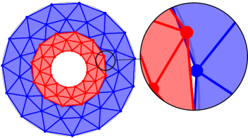
Figure 1: Schematic visualization of element mismatch at the interface between rotor (red) and stator (blue) the circular interface is not exactly represented by the mesh.

All ‘sliding’ methods share the the problem of geometric mismatch at the interface, see Figure 1. This may lead to numerical noise which is particular cumbersome when analyzing cogging torque. When using conventional finite elements this can be mitigated by mesh adaptation, see [10, Section 5.4] and similarly [5, Section 5.2.3]. The geometry error can be avoided when using Isogeometric Analysis (IGA) [11] which uses B-Splines and Non-Uniform Rational B-Splines (NURBS) for both the geometry representation (as weighting functions on a structured list of control points, defining a control mesh) and as basis functions for test-spaces and discretization. Classically, a conforming multipatch discretization is needed for IGA [12]. While IGA has been used for machine models in the past, e.g., [13, 14, 15], this paper presents the first isogeometric simulation workflow for rotating machines with focus on torque computation. To implement rotation efficiently, we extend the isogeometric mortar method from [16] and use a tree-cotree regularization [17].

The paper is structured as follows; we discuss the mathematical model in Section II and the discretization using IGA in Section III. Mortaring and tree-cotree regularization are introduced in Sections III-A and III-B, respectively. Different methods for torque computation are given in Section IV. Finally, numerical results are presented in Section V and the paper is closed by conclusions in Section VI.

II Mathematical Machine Model

The electromagnetic behavior of electric machines can be described by Maxwell’s equations. Under common assumptions, the magnetostatic approximation can be employed. Using a magnetic vector potential $\mathbf{A}$, such that $\mathbf{B}=\operatorname{curl}\mathbf{A}$, the problem in a 3D domain $\Omega$ can be written as curl(νcurl A ) = J_src + curl M , where $\nu$ is the magnetic reluctivity, $\mathbf{J}_{\mathrm{src}}$ is a source current density and $\mathbf{M}$ is the magnetization of permanent magnets. The weak formulation can be derived as: find $\mathbf{A}\in V$, s.t.

$$\aligned(\nu\operatorname{curl}\mathbf{A},\operatorname{curl}\mathbf{v})_{\Omega}-(\nu\operatorname{curl}\mathbf{A}\times\mathbf{n},\mathbf{v})_{\partial\Omega}\\ =(\mathbf{J}_{\mathrm{src}},\mathbf{v})_{\Omega}-(\mathbf{M},\operatorname{curl}\mathbf{v})_{\Omega},$$ (1)

for all basis functions $\mathbf{v}\in V$, where $V\subset{H}(\mathrm{curl};\Omega)$, fulfill the boundary conditions on $\partial\Omega$.

Let us consider the case of a circular rotating machine. We introduce a cut within the air gap $\Omega_{\mathrm{air}}$ decomposing the domain into $\Omega=\Omega_{1}\cup\Omega_{2}$ for stator/rotor. We call the interface $\Gamma_{12}=\partial\Omega_{1}\cap\partial\Omega_{2}\subset\Omega_{\mathrm{air}}$ with normal vector $\mathbf{n}_{12}$ and denote the air gap pieces by $\Omega_{\mathrm{air},i}=\Omega_{i}\cap\Omega_{\mathrm{air}}$. The angle $\alpha$ encodes the angular offset between rotor and stator due to motion. Then, we may choose any closed surface $S$ that is contained in the air gap, e.g., the lateral cylinder surface $S=\Gamma_{12}$ to compute the torque, [18, p. 55f]. It can be parametrized conveniently by a cylindrical coordinate system with (constant) radial distance $r=R$, angle $\theta\in[0,2\pi]$ and axial coordinate $z\in[0,l_{z}]$ where $l_{z}$ is the length of the machine. Now, the torque can be computed as the surface integral, see e.g. [18, eq. (121)]

$$T_{\theta}(\alpha)=\int\limits_{0}^{l_{z}}\int\limits_{0}^{2\pi}B_{r}(\alpha)H_{\theta}(\alpha)R^{2}\;\mathrm{d}\theta\;\mathrm{d}z,$$ (2)

where $B_{r}(\alpha)$ and $H_{\theta}(\alpha)$ are the radial and angular components of the magnetic flux density $\mathbf{B}$ and field strength $\mathbf{H}=\nu\mathbf{B}$ for each rotor angle $\alpha$, respectively. Note, that we dropped the spatial coordinates and transforms for readability.

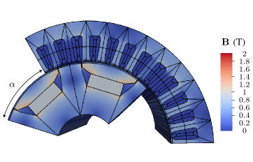
Figure 2: Magnetic flux density in two poles of a six-pole permanent magnet synchronous machine with angle $\alpha$, computed using isogeometric mortaring.

III Isogeometric Analysis

The geometry is defined by one or several trivariate B-splines or NURBS mappings [19] from a reference domain $\hat{\Omega}=(0,1)^{3}$ to the physical domain $\Omega$. For geometries which cannot be represented by a regular mapping a conforming multipatch model can be used where the geometry of each patch is defined by a separate trivariate mapping. Following the usual notation, B-splines of degree $p$ are defined from the knot vector

$$\Xi=\left[\xi_{1},\dots,\xi_{n+p+1}\right]\quad 0\leq\xi_{i}\leq\xi_{i+1}\leq 1,$$ (3)

using the Cox-De Boor recursion formula [19], where $n$ is the number of functions. Let us denote by $\hat{B}_{i}^{p}$ the $i$-th basis function of degree $p$ on the reference domain $(0,1)$ and define the trivariate space of B-splines as

$$\aligned S_{p_{1},p_{2},p_{3}}&(\Xi_{1},\Xi_{2},\Xi_{3})=\\ \mathrm{span}\left\{\prod_{k=1}^{3}\hat{B}_{i_{k}}^{p_{k}}(\Xi_{k})\;\Big{|}\;1\leq i_{k}\leq n_{k}\right\}.$$ (4)

As we need edge element basis functions for the solution of eq:weakMagnetostatic, we require a curl-conforming spline space. For simplicity we assume that the polynomial degree is the same in all parametric directions, i.e., $p=p_{1}=p_{2}=p_{3}$. Following [16], we define the corresponding spline space in the reference domain $\hat{\Omega}$ as

$$\aligned S_{p}^{1}(\hat{\Omega})&=S_{p-1,p,p}(\Xi_{1}^{\prime},\Xi_{2},\Xi_{3})\\ \times S_{p,p-1,p}(\Xi_{1},\Xi_{2}^{\prime},\Xi_{3})\\ \times S_{p,p,p-1}(\Xi_{1},\Xi_{2},\Xi_{3}^{\prime}),$$ (5)

where $\Xi_{j}^{\prime}=[\xi_{2}^{j},\dots,\xi_{n_{j}+p}^{j}]$ for $j=1,2,3$ is a modified knot vector with the first and last knot removed. This corresponds to lowering the degree and regularity of the basis functions by one in the $j$-th direction. Then, considering the geometry mappings and their Jacobians, the multipatch spline spaces in the physical domain $\Omega$ are defined by push-forwards. We obtain

$$V:=S_{p}^{1}(\Omega),\quad M_{12}:=\boldsymbol{\gamma}_{\perp,\Gamma_{12}}(S_{q}^{1}(\Omega_{1})),$$ (6)

with the trace operator $\boldsymbol{\gamma}_{\perp,\Gamma_{12}}(\mathbf{u}):=\mathbf{u}\times\mathbf{n}_{12}$ restricted to $\Gamma_{12}$. A stable mortar space $M_{12}$ for the multiplier can be easily created by lowering its degree by an odd number with respect to the edge-element space of the vector potential, e.g., $q=p-1$ by removing knots from eq:knot. Boundary conditions on $\partial\Omega$ may still be implemented. Note that these spline spaces are part of a de Rham complex [16].

III-A Mortaring

Stator $\Omega_{1}$ and rotor $\Omega_{2}$ are modeled independently and are glued for angle $\alpha$ using our isogeometric mortar method [16]. Note that we will drop the $\alpha$ dependency for readability if possible. The coupling is realized by introducing a Lagrange multiplier λ = νcurl A ×n_12, to eq:weakMagnetostatic, where $\mathbf{n}_{12}$ is the normal vector on $\Gamma_{12}$, yielding the following problem: find $\mathbf{u}\in V$, $\boldsymbol{\boldsymbol{\lambda}}\in M_{12}$ such that a(u, v)_Ω + b(v, λ)_Γ_12 &= f(v)_Ω
b(u, μ)_Γ_12 = 0 for all $\mathbf{v}\in V$ and $\boldsymbol{\mu}\in M_{12}$ and the bilinear forms a(u, v)_Ω &:= ∑_k=1^2 (νcurl u, curl v)_Ω_k,
b(u, μ)_Γ_12 := ([γ_12(u)], μ)_Γ_12 and right-hand-side f(v)_Ω := ∑_k=1^2 (J_src,v)_Ω_k - (M , curlv)_Ω_k where $\boldsymbol{\gamma}_{12}(\mathbf{u})=(\mathbf{n}_{12}\times\mathbf{u})\times\mathbf{n}_{12}$ and the brackets $[\cdot]$ denote the jump across the interface $\Gamma_{12}$.

Spectral correctness and inf-sup stability of the saddle-point problem (III-A-III-A) for adequate choices of the spaces have been recently proven in [16]. This is a significant advantage of isogeometric mortaring compared to other mortar variants, e.g., using conventional finite elements with rather complicated constructions of dual basis functions. One key issue is the construction of an intersection mesh in the reference domain $\hat{\Gamma}$ for the numerical quadrature of the integral eq:quadrature, see Fig. 3. This is also straightforward due to the tensor product structure of the spaces.

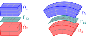
Figure 3: Schematic visualization of the mesh of the reference domains $\hat{\Omega}_{1}$, $\hat{\Omega}_{2}$ and the intersection mesh on the interface $\hat{\Gamma}_{12}$ on the left and of the physical domains ${\Omega}_{1}$, ${\Omega}_{2}$ and the intersection mesh on the interface ${\Gamma}_{12}$ on the right.

III-B Tree-Cotree Regularization

The removal of the (discrete) kernel of the curl operator is a necessary requirement for the well-posedness of formulation eq:weak1–eq:weak2. In particular, the matrix discretizing eq:curlcurl_bf will be singular on each subdomain of the domain decomposition. A popular way to amend the issue in low order FEM ($p=1$) is to set the solution a priori on the spanning tree of edges in the vertex-edge mesh graph. This works because of the discrete degrees of freedom (DoFs) correspondence to line integrals on edges of the FEM mesh, which in turn easily permits to identify the gradient subspace of $V$.

Unfortunately, in the IGA setting just as in FEM, as soon as $p>1$, the DoFs of $V$ will lose their physical interpretation. Nevertheless, as noted in the literature [20] the basis functions of the spline spaces $S_{p}^{k}(\Omega)$ in the discrete de Rham sequence can be identified with $k-$dimensional entities of the underlying piecewise affine control mesh, i.e., with vertices, edges, facets, and cells for $k=0,1,2$ and $3$, respectively. Because of these one-to-one correspondences, it suffices to apply the algorithm for the tree and cotree construction to the control mesh graph itself, and identify the corresponding B-spline functions. Very conveniently, this observation holds also for different boundary conditions and in the case of non-contractible domains. In this last case we can apply the techniques used to identify generators of cohomology groups for low order schemes in [21] to the standard tree-cotree decomposition. Finally, the extension to mortaring is described in [17].

IV Torque Calculation

In our mortaring setting, one easily verifies that the third component of the Lagrange multiplier $\lambda_{3}=-H_{\theta}$ can be identified with the (negative) angular component of the magnetic field strength. Therefore, we can immediately compute the torque by

$$T_{\theta}(\alpha)=-\int\limits_{0}^{l_{z}}\int\limits_{0}^{2\pi}B_{r}(\alpha)\lambda_{3}(\alpha)R^{2}\;\mathrm{d}\theta\;\mathrm{d}z$$ (7)

when evaluating $B_{r}=\operatorname{curl}(\mathbf{A})\cdot\mathbf{n}_{12}$ either on the boundary of $\Omega_{1}$ (stator) or $\Omega_{2}$ (rotor). Note that the corresponding numerical quadrature (on patch boundaries in the reference domain $\hat{\Omega}$) is straight forward since we are integrating on a perfect cylindrical shape. However, such direct evaluation of eq:torque is commonly considered numerically unstable [18, p. 55], i.e., the result is very sensitive with respect to the choice of the integration interface $S$. Therefore a large variety of methods and formulae to calculate the electromagnetic torque has been developed, a comprehensive literature review is given in [22]. A particular popular variant is Arkkio’s method which averages the torque over some volume, i.e.,

$$T_{\theta}(\alpha)=\int\limits_{0}^{l_{z}}\int\limits_{0}^{\delta}\int\limits_{0}^{2\pi}B_{r}(\alpha)H_{\theta}(\alpha)(R+r)^{2}\;\mathrm{d}\theta\;\mathrm{d}r\;\mathrm{d}z.$$ (8)

where we can, for example, evaluate the fields either in the air gap contained in $\Omega_{\mathrm{air},1}$ (stator) or $\Omega_{\mathrm{air},2}$ (rotor).

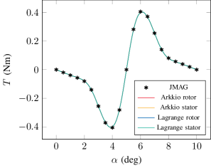
Figure 4: Torque computations via reference 2D FE solution (JMAG), Arkkio’s method (8) on rotor and stator side (Arkkio rotor/stator), Lagrange multipliers method (7) on rotor and stator side (Lagrange rotor/stator).

V Numerical Results

The isogeometric mortaring described in (III-A-III-A) is used to compute the magnetic field of a six-pole permanent magnet synchronous machine, whose details are given in [15]. Degree $p=2$ is used for the discrete edge element spaces $V$ and $q=1$ for the multiplier space $M_{12}$ which is defined on the interface mesh of $\Omega_{1}$. The rotor consists of 24 patches, resulting in 540353 cotree DoFs (and 309663 eliminated tree DoFs), the stator is given by 228 patches and 1058880 cotree DoFs (and 601392 eliminated tree DoFs), the multiplier adds another 3912 DoFs. The model and magnetic flux density in this machine can be seen in Fig. 2. The cogging torque is computed using the Lagrange multipliers (7) and Arkkio’s method (8) on $\Omega_{1}$ (stator) and $\Omega_{2}$ (rotor), respectively. In Arkkio’s method the integration volume is chosen in both cases as the whole air gap piece $\Omega_{\mathrm{air},i}$. The results are shown in Fig. 4 and compared to a 2D reference solution computed using JMAG^® with a finite element discretization of order $p=1$ with 1618173 elements. The difference between the torque computed with the IGA approaches and the JMAG reference solution is shown in Fig. 5. All approaches are in excellent agreement. We do not observe the often reported instability for surface/line evaluation of the torque. In our approach, the cylindrical shape of the machine can be exactly described and the angular component of the magnetic field can be obtained from the Lagrange multipliers alleviating the need to numerically differentiate the magnetic vector potential for this component.

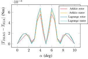
Figure 5: Absolute difference between the torque computed via reference 2D FE solution (JMAG) and the torque computed with IGA using Arkkio’s method (8) on rotor and stator side (Arkkio rotor/stator), Lagrange multipliers method (7) on rotor and stator side (Lagrange rotor/stator).

VI Conclusion

We have introduced isogeometric mortaring for rotating electric machines using a tree-cotree decomposition for the regularization of the system. Two different methods for the torque computation of electric machines have been introduced and used for the computation of the cogging torque of a 3D six-pole permanent magnet synchronous machine. Isogeometric analysis and in particular isogeometric mortaring were demonstrated to be very well suited for the torque computation. Surface and volume integration for the evaluation of the torque are in excellent agreement with a reference solution.

References

- [1] P. T. Boggs, A. Althsuler, A. R. Larzelere, E. J. Walsh, R. L. Clay, and M. F. Hardwick, “DART system analysis,” Sandia National Laboratories, Technical Report, Aug. 2005.
- [2] H. De Gersem and T. Weiland, “Harmonic weighting functions at the sliding interface of a finite-element machine model incorporating angular displacement,” IEEE Trans. Magn., vol. 40, no. 2, pp. 545–548, Mar. 2004.
- [3] B. Davat, Z. Ren, and M. Lajoie-Mazenc, “The movement in field modeling,” IEEE Trans. Magn., vol. 21, no. 6, pp. 2296–2298, Nov. 1985.
- [4] H. C. Lai, D. Rodger, and P. J. Leonard, “Coupling meshes in 3D problems involving movements,” IEEE Trans. Magn., vol. 28, no. 2, pp. 1732–1734, Mar. 1992.
- [5] G. J. Wallinger, “A method to couple non-conforming finite element meshes,” Dissertation, TU Graz, 2019.
- [6] S. Kurz, J. Fetzer, and G. Lehner, “An improved algorithm for the BEM-FEM-coupling method using domain decomposition,” IEEE Trans. Magn., vol. 31, no. 3, pp. 1737–1740, 1995.
- [7] K. Roppert, S. Schoder, F. Toth, and M. Kaltenbacher, “Non-conforming Nitsche interfaces for edge elements in curl–curl-type problems,” IEEE Trans. Magn., vol. 56, no. 5, pp. 1–7, 2020.
- [8] A. Buffa and F. Rapetti, “A sliding mesh-mortar method for a two-dimensional eddy currents model of electric engines,” M2AN, 1999.
- [9] F. Bouillault, A. Buffa, Y. Maday, and F. Rapetti, “The mortar edge element method in three dimensions: applications to magnetostatics,” SIAM J. Sci. Comput., vol. 24, no. 4, pp. 1303–1327, 2001.
- [10] E. Lange, “Numerische Werkzeuge zur Simulation von nichtsinusförmig gespeisten geregelten elektrischen Maschinen im dynamischen Betrieb,” Dissertation, RWTH Aachen, Dec. 2012.
- [11] T. J. R. Hughes, J. A. Cottrell, and Y. Bazilevs, “Isogeometric analysis: CAD, finite elements, NURBS, exact geometry and mesh refinement,” CMAME, vol. 194, pp. 4135–4195, 2005.
- [12] A. Buffa, R. H. Vázquez, G. Sangalli, and L. B. da Veiga, “Approximation estimates for isogeometric spaces in multipatch geometries,” Numer. Meth. Part. Differ. Equat., vol. 31, no. 2, pp. 422–438, 2015.
- [13] Z. Bontinck, J. Corno, S. Schöps, and H. De Gersem, “Isogeometric analysis and harmonic stator-rotor coupling for simulating electric machines,” CMAME, vol. 334, pp. 40–55, 2018.
- [14] L. A. J. Friedrich, B. L. J. Gysen, J. W. Jansen, and E. A. Lomonova, “Analysis of motional eddy currents in the slitted stator core of an axial-flux permanent-magnet machine,” IEEE Trans. Magn., vol. 56, no. 2, pp. 1–4, 2020.
- [15] M. Merkel, P. Gangl, and S. Schöps, “Shape optimization of rotating electric machines using isogeometric analysis,” IEEE Trans. Energ. Convers., Feb. 2021.
- [16] A. Buffa, J. Corno, C. de Falco, S. Schöps, and R. Vázquez, “Isogeometric mortar coupling for electromagnetic problems,” SIAM J. Sci. Comput., vol. 42, no. 1, pp. B80–B104, Jan. 2020.
- [17] B. Kapidani, M. Merkel, S. Schöps, and R. Vázquez, “Tree-cotree decomposition of isogeometric mortared spaces in h(curl) on multi-patch domains,” Cornell University, Preprint arxiv:2110.15860, 2021.
- [18] A. Arkkio, “Analysis of induction motors based on the numerical solution of the magnetic field and circuit equations,” PhD Thesis, Helsinki University of Technology, 1987.
- [19] E. Cohen, R. F. Riesenfeld, and G. Elber, Geometric Modeling with Splines: An Introduction. CRC Press, 2001.
- [20] L. Beirão da Veiga, A. Buffa, G. Sangalli, and R. Vázquez, “Mathematical analysis of variational isogeometric methods,” Acta Numerica, vol. 23, pp. 157–287, May 2014.
- [21] P. Dlotko, B. Kapidani, and R. Specogna, “Topoprocessor: An efficient computational topology toolbox for h-oriented eddy current formulations,” IEEE Trans. Magn., vol. 53, no. 6, pp. 1–4, Jun. 2017.
- [22] F. Henrotte, M. Felden, M. van der Giet, and K. Hameyer, “Electromagnetic force computation with the eggshell method,” in 14th International IGTE Symposium,2010.