Parameter uncertainty estimation for exponential semi-variogram models: Two generalized bootstrap methods with check- and quantile-based filtering

Abstract

Estimation of parameter standard errors for semi-variogram models is challenging, given the two-step process required to fit a parametric model to spatially correlated data.

Motivated by an application in social epidemiology, we focus on exponential semi-variogram models fitted to data with 500 to 2000 observations and little control over the sampling design. Previously proposed methods for the estimation of standard errors cannot be applied in this context. Approximate closed form solutions are too costly using generalized least squares in terms of memory capacities. The generalized bootstrap proposed by Olea and Pardo-Igúzquiza is nonetheless applicable with weighted instead of generalized least squares. However, the standard error estimates are hugely biased and imprecise.

Therefore, we propose to add a filter mechanism to the generalized bootstrap. The new development is presented and evaluated with a simulation study which shows that the generalized bootstrap with check-based filtering leads to massively improved results compared to the generalized bootstrap method without filtering. We provide a case study using birthweight data.

1 Introduction

1.1 Contextual background

Semi-variogram modelling is a method used in spatial statistics to model the relationship between pairwise correlation of observations and the distance between these observations. It is commonly used in fields like agriculture or ecology but has also seen applications in social epidemiology to study neighbourhood effects on health. In the latter, the estimation of exponential parametric models is of particular interest because it provides a measure of which part of the total variance is spatially structured and which local spatial scale is relevant. However, the assessment of parameter uncertainty presents some difficulties while being necessary for proper inference [1].

Contrary to some other fields of application, data in social epidemiology cannot be sampled according to a scheme designed to facilitate the estimation of parameters. On the contrary, analyses are usually based on survey data in which there are few observations at very small distances [2] - providing very few data for the estimation of the first points of the empirical semi-variogram - but with possibly large sample sizes of over 1000 - making, for instance, inverting matrices for the estimation of standard errors difficult. Exemplary applications of semi-variogram modelling in this context can be found in [2] and [3].

1.2 Technical challenges

Three characteristics of semi-variogram estimation are a source of technical difficulties for the construction of parameter estimators and, thereby, for the construction of parameter uncertainty estimators. First, the estimation of parameters associated with correlated data has to take the correlation structure into account. Consequently, the simplifying assumption of an underlying data generating process with independent and identically distributed elements is not appropriate [4, p.3]. Second, the estimation of the semi-variogram is not based on the spatial observations themselves but on their pairwise Euclidean distances [5]. Third, the fitting of a semi-variogram model requires a two-step process that includes, first, the estimation of a discrete semi-variogram and, second, based on that the fitting of a mostly continuous model. Multiple steps of transformation and estimation intuitively lead to multiple potential sources of uncertainty that influence the precision of the semi-variogram model parameters.

1.3 Existing approaches

Methods for the parameter standard error estimation have been proposed in the past.

An analytic solution was developed by Pardo-Igúzquiza and Dowd [6] for Gaussian data generating processes. Parameter estimates are obtained using the generalized least squares (GLS) estimation approach. While it leads to reliable standard error estimates for datasets with up to 100 observations, results are often not obtained for larger sample sizes of 1000 or higher due to the at least quadratically increasing amount of memory capacities required for the computation. Moreover, the theoretical statistical assumptions made in order to construct the analytic solution are often not fulfilled such that solutions, if feasible, have to be interpreted to be approximate rather than exact.

An empirical approach using the so called generalized bootstrap is provided by Olea and Pardo-Igúzquiza [7]. The reduced amount of theoretical assumptions and the use of the bootstrap approach which can be implemented quite efficiently are advantageous. However, as for the previous method, the generalized bootstrap is originally constructed with focus on data with less than 100 observations, high control over the sampling design and locations, and parameter estimates obtained with the GLS approach as is typically the case in the geological context. Larger datasets and the often conducted parameter estimation based on bootstrap samples have forced us to substitute the GLS parameter estimation by the weighted least squares (WLS) estimation procedure in order to make it computationally feasible with our data. Given these changes, the standard error estimates are highly biased upwards and very imprecise.

A more recent attempt by Saha and Datta [8] uses an approximate maximum likelihood estimation algorithm with sparse distance matrices for the parameter estimation to fasten the computation procedure of the standard error estimates via generalized bootstrap. The approach focuses on applications to very large datasets with 10000 or more data points and assumes approximate Gaussianity for the maximum likelihood estimation. Datasets with a sample size of about 1000 appear to be too small to account for the errors due to sparse computation, so that the semi-variogram parameter estimators themselves are hugely biased and therefore not an appropriate base for uncertainty estimation.

1.4 Extension of the generalized bootstrap approach

A difficulty associated with the used of bootstrap methods to estimate the uncertainty of parameter estimates is that the fitting of a parametric model to an empirical semi-variogram requires tuning of metaparameters and a visual check of the fit. The latter cannot be performed by a bootstrap and may lead to an overestimation of the the variability of estimates. It follows that estimating standard errors based on one of the existing methods does not provide satisfactory results in the data scenarios of our interest.

Focusing on typical social epidemiological data to which exponential semi-variogram models are to be fitted, we need a standard error estimation tool that

1. works under as few distributional assumptions as possible,

2. is based on the commonly used and computationally feasible WLS model fitting approach,

3. is applicable to data with sample sizes of about 500 to 2000 and little or no control over the sampling design,

4. is less biased and more stable that the methods available.

We propose to use the generalized bootstrap by Olea and Pardo-Igúzquiza [7] using WLS rather than GLS for standard error estimation. To compensate for the higher variance of the standard error estimator that is observed in simulations representing the scenarios of our interest, the generalized bootstrap procedure is extended by a filter. The filter evaluates each bootstrap estimate and excludes results of a bootstrap estimation if the semi-variogram model fitting algorithm is suspected to have not converged or provides an estimate which is a poor fit of the empirical semi-variogram. Two filter options are presented and evaluated: the check-based filtering and the quantile-based filtering.

2 Methods

2.1 Statistical model

We assume an isotropic and second-order stationary spatial process $\{Z(\mathbf{s})\mid\mathbf{s}\in D\}$ with a collection of random variables $Z(\mathbf{s})$ and a set of locations $D$. In this case, the semi-variogram of a spatial process characterizes the semi-variance structure of the process depending on the Euclidean distance $h=||\mathbf{s}-\mathbf{s}^{\prime}||$ between two subjects [9, p.135–140]. The semi-variogram is defined as

$$\gamma(h)=\frac{1}{2}Var(Z(\mathbf{s})-Z(\mathbf{s}^{\prime}))$$ (1)

for two subjects at locations $\mathbf{s}$ and $\mathbf{s}^{\prime}$ with distance $h:=||\mathbf{s}-\mathbf{s}^{\prime}||$.

Under the stated conditions the semi-variogram and the covariance function of the spatial process have the relationship:

$$C(h)=c_{0}+\sigma_{0}^{2}-\gamma(h)$$ (2)

where $c_{0}+\sigma_{0}^{2}=Var[Z(\mathbf{s})]$ is the variance of the outcome to be analysed. It is assumed to be constant over the studied surface. The summand $c_{0}$ is called nugget effect and defines the value of $\gamma(h)$ for $h$ approaching zero. The so called partial sill $\sigma_{0}^{2}$ describes the asymptotic covariance of two observations on the same location.

Given data, Matheron’s estimator provides an unbiased empirical estimate of the semi-variogram [10]. It is defined as

$$\hat{\gamma}(h)=\frac{1}{2\cdot|N(h)|}\sum_{(\mathbf{s_{i}},\mathbf{s_{j}})\in N(h)}\{Z(\mathbf{s_{i}})-Z(\mathbf{s_{j}})\}^{2},$$ (3)

where $N(h):=\{(\mathbf{s_{i}},\mathbf{s_{j}})\in D|\;\;||\mathbf{s_{i}}-\mathbf{s_{j}}||=h\}$. To guarantee a sufficient cardinality of $N(h)$ for each realized $h$, multiple lag distances are grouped into lag intervals of the form $[h-\varepsilon,h+\varepsilon]$ for a discrete number of lags $h_{1},\dots,h_{K}$.

Whereas the empirical semi-variogram provides point estimates for a finite number of lag intervals, an almost continuous model is obtained by a parametric semi-variogram model. The exponential semi-variogram model is defined as

$$\gamma_{\text{exp}}(h;c_{0},\sigma^{2}_{0},\phi)=c_{0}+\sigma_{0}^{2}\Big{\{}1-\exp\big{(}-\frac{h}{\phi}\big{)}\Big{\}}\;\; \text{for}\;\;h>0$$ (4)

and $\gamma_{\text{exp}}(h;c_{0},\sigma^{2}_{0},\phi)=0$ for $h=0$ with nugget effect $c_{0}>0$, partial sill $\sigma_{0}^{2}>0$ and range parameter $\phi>0$ [4, p.61].

2.2 Model fitting

The semi-variogram model fitting is commonly done via the method of WLS or GLS [9, p.163–166]. In both cases the parameter vector $\theta=(c_{0},\sigma_{0}^{2},\phi)^{t}$ that minimizes the loss function

$$LOSS(\theta)=[\hat{\mathbf{\gamma}}-\mathbf{\gamma_{\text{exp}}(\theta)}]^{t}\;\mathbf{\Gamma}^{-1}\;[\hat{\mathbf{\gamma}}-\mathbf{\gamma_{\text{exp}}(\theta)}]$$ (5)

is chosen. The vector $\hat{\mathbf{\gamma}}=(\hat{\gamma}(h_{1}),\dots,\hat{\gamma}(h_{K}))^{t}$ contains the empirical semi-variogram evaluated at $K$ lag distances and $\mathbf{\gamma_{\text{exp}}(\theta)}=(\gamma_{\text{exp}}(h_{1};\mathbf{\theta}),\dots,\gamma_{\text{exp}}(h_{K};\mathbf{\theta}))^{t}$ is the corresponding semi-variogram model evaluated at the same lag distances. To fit a model $\gamma_{\text{exp}}$ to the empirical semi-variogram $\hat{\gamma}$ an estimate for the covariance matrix of the empirical semi-variogram denoted by $\mathbf{\Gamma}\in\mathbb{R}^{K\times K}$ is needed.

In case of the GLS estimation method, varying variances of the lags’ semi-variogram estimates are allowed, as well as covariances between two lags. This is reflected by a $\mathbf{\Gamma}$ matrix with potentially non zero entries on the diagonal and off-diagonal [11] and can be expected to lead to very precise results. However, the computational effort regarding the memory capacities increases at minimum quadratically with the sample size $N$ since the number of pairwise distances that go into the estimation of $\mathbf{\Gamma}$ increases proportionally to $N^{2}$ making calculations for large N infeasible.

Therefore, the WLS method will be used as next best and applicable solution for the semi-variogram parameter estimation. In case of the WLS estimation method, $\mathbf{\Gamma}$ is a diagonal matrix with varying entries and thus assumes varying variances for each lag’s estimate. The covariances between two lags is preset to be zero. We choose weights depending on the number of data pairs that are considered for the estimation of the empirical semi-variogram according to Matheron’s estimator and the middle lag distance assigned to each lag interval. The covariance matrix estimate has entries $\mathbf{\Gamma}_{kk}=h^{2}_{k}/|N(h_{k})|$ on the diagonal and $\mathbf{\Gamma}_{kl}=0$ on the non-diagonal for $k,l=1,\dots,K$ and $k\not=l$. Thereby, minimizing the difference between empirical semi-variogram and model at lag distances with more information and at smaller lag distances is prioritized. The general formula of the loss function to be minimized then reduces to

$$LOSS_{\text{WLS}}(\theta)=\sum_{k=1}^{K}\frac{|N(h_{k})|}{h_{k}^{2}}\;\cdot[\hat{\gamma(h_{k})}-\gamma_{\text{exp}}(h_{k};\theta)]^{2}$$ (6)

which is implemented in the fit.variogram function from within the Rpackage gstat [12] with the default argument fit.method=7 [13].

2.3 Generalized bootstrap with filtering

The generalized bootstrap approach [7] serves as starting point, but requires modification to be applicable in the stated data framework of our interest. Each semi-variogram model is fitted using the WLS instead of the GLS method. Moreover, substantial changes are made with respect to the purpose of the bootstrap estimates. Whereas the original algorithm’s goal is the estimation of the covariance matrix and confidence bands of the empirical semi-variogram for each defined lag interval, the focus here lies on the estimation of model parameter standard errors of a fitted exponential semi-variogram model. As a completely new element, a filter within the bootstrapping process tackles the exclusion of improbable bootstrap estimates due to non-convergence of the semi-variogram model fitting algorithm.

Considering these aspects, the following algorithm was developed:

1. Exponential semi-variogram model: An empirical semi-variogram is estimated based on the original spatial dataset $\mathbf{z}=(z_{1},\dots,z_{N})^{t}$ plus the spatial coordinates $\mathbf{s}$ with $\mathbf{s_{i}}\in\mathbb{R}^{2}$ for $i=1,\dots,N$. Subsequently, an exponential semi-variogram model $\gamma_{\text{exp}}$ is fitted using the WLS method producing the parameter estimate $\mathbf{\hat{\theta}}$ for the true parameter vector $\mathbf{\theta}=(c_{0},\sigma^{2}_{0},\phi)^{t}$.

2. Normal score transformation: The data vector $\mathbf{z}$ is mapped into a Gaussian space by the empirical normal score transformation function $\varphi$ that maps the data from the attribute space into a Gaussian space. Consequently, $\mathbf{y}=\varphi(\mathbf{z})$ is a realization vector of a standard normal random variable [14, 15].

3. Exponential semi-variogram model for transformed data: An empirical semi-variogram is fitted to $\mathbf{y}$ combined with the original data coordinates. Based on that, an exponential semi-variogram model $\tilde{\gamma}_{\text{exp}}$ is fitted using the WLS method providing the parameter estimate $\mathbf{\tilde{\theta}}$.

4. Covariance estimation: Making use of the semivarigram model $\tilde{\gamma}_{\text{exp}}$, the covariance between two data points $z_{i}$ and $z_{j}$ is calculated based on their Euclidean distance $d_{ij}=d(s_{i},s_{j})$ as

   $$c_{ij}=\tilde{c_{0}}+\tilde{\sigma}_{0}^{2}-\tilde{\gamma}_{\text{exp}}(d_{ij}).$$ (7)

   The $N\times N$ covariance matrix with entries $c_{ij}$ is denoted as $\mathbf{C}$.

5. Decorrelation of the data: The decomposition of the covariance matrix $\mathbf{C}$ into the product of the lower triangular matrix $\mathbf{L}$ and its transposed is obtained by the Cholsky decomposition algorithm as

   $$\mathbf{C}=\mathbf{L}\mathbf{L}^{t}.$$ (8)

   This is possible because $\mathbf{C}$ is square symmetric and positive-definite [16]. The vector

   $$\mathbf{x}=\mathbf{L}^{-1}\mathbf{y}$$ (9)

   is a set of independent and identically distributed, hence uncorrelated values.

6. Classical bootstrap: Sampling $N$ times with replacement from $\mathbf{x}$ generates a bootstrap sample $\mathbf{x^{*}}$.

7. Recorrelation: The bootstrap sample $\mathbf{x^{*}}$ reinherits the correlation structure by applying the inverse operation of step 4, that is

   $$\mathbf{y^{*}}=\mathbf{Lx^{*}}.$$ (10)

8. Normal score back transformation: The back transformation of $\mathbf{y^{*}}$ to the attribute space through the inverse normal score function in step 1 is done by

   $$\mathbf{z^{*}}=\varphi^{-1}(\mathbf{y^{*}}).$$ (11)

9. Analysis of the bootstrap sample: An exponential semi-variogram model is estimated based on $\mathbf{z^{*}}$ combined with the original coordinates providing an estimate $\mathbf{\theta^{*}}$.

From here on, the algorithm depends on the choice of filter method. If the check-based filter is used, steps 9c, 10c and 11 are executed.

1. Check-based filtering: A test is applied to the bootstrap estimate $\theta^{*}$ to indicate whether the exponential semi-variogram fitting algorithm did converge. If the algorithm is assumed to have failed, the bootstrap estimate is discarded.

2. Repetition: The steps 5 to 9 are repeated until a set of $B$ bootstrap estimates ${\{\theta^{*}_{b}\}}_{b=1,\dots,B}$ has aggregated.

If the quantile-based filter is used, steps 9q, 10q and 11 are conducted.

1. Repetition: Given the quantile threshold $\alpha\in(0,1)$, the steps 5 to 8 are repeated $\tilde{B}=\frac{1}{\alpha}\cdot B$ times providing a set of $\theta^{*}_{b}$ for $b=1,\dots,\tilde{B}$.

2. Quantile-based filtering: The first $B$ values of the increasingly ordered set of bootstrap estimates $\theta^{*}_{b}$ is saved. This equals the set of bootstrap estimates between the minimum value and the $\alpha$-quantile.

3. Parameter standard error estimation: Based on the filtered set of bootstrap estimates $\mathbf{\theta}^{*}_{b}$ for $b=1,\dots B$ the parameter standard error estimates are defined as

   $$\widehat{\eta_{\theta_{j}}}=sd(\theta^{*}_{j})=\sqrt{\frac{1}{B-1}\sum_{b=1}^{B}\Big{\{}\theta_{bj}^{*}-\overline{\theta_{j}^{*}}\Big{\}}^{2}},$$ (12)

   for $j=1,...,3$ referring to the three parameters $c_{0},\sigma^{2}_{0},\phi$.

2.3.1 Check-based filtering

The check-based filter (steps 9c, 10c) is applied in each repetition. The bootstrap estimate $\theta^{*}$ is used to compute the corresponding overall variance according to the model as $c_{0}^{*}+\sigma_{0}^{2*}$. If

$$c_{0}^{*}+\sigma_{0}^{2*}>\tau Var(\mathbf{z})\;\;\text{or}\;\;\phi^{*}<0,$$ (13)

i.e. if the variance indicated by the model exceeds the sample variance times some threshold factor $\tau$ or the shape parameter lies outside its constraint, the bootstrap estimate $\theta^{*}$ is discarded. Experience has shown that the WLS algorithm sometimes leads to shape parameter estimates outside its constraint. Otherwise, it is retained. The size of the bootstrap sample $B$ is specified beforehand and the procedure of estimating and checking one bootstrap estimate is repeated until $B$ bootstrap estimates are accepted.

2.3.2 Quantile-based filtering

For each bootstrap estimation, we check whether the parameter constraint $\phi^{*}>0$ is complied during the WLS estimation. After the computation of all bootstrap estimates the quantile-based filter (steps 9q, 10q) is applied. Given a threshold percentile $\alpha$ all bootstrap estimates $\theta^{*}_{b}$ beyond the $\alpha\cdot 100\%$-quantile $q_{\alpha}(\theta^{*}_{j})$ for $j=1,2,3$ are discarded while all bootstrap estimates up to the $\alpha\cdot 100\%$-quantile are saved.

To make sure the set of bootstrap estimates used for the computation of the parameter standard error contains $B$ elements, the number of bootstrap samples to be generated in the first place is set to $\tilde{B}=B\cdot\frac{1}{\alpha}$.

3 Simulation study

A simulation study is conducted in order to test and evaluate the performance of the presented filter methods in various sampling frameworks and provide recommendations for meta- and tuning parameter specification. The implementation is constructed using the statistical software environment R [17]. The R package gstat [12] is used to simulate spatial data. The packages gstat [12], SpatialTools [18] and additional individual functions [15] are used for the implementation of the generalized bootstrap algorithm with each filter method. The algorithms and simulation code are stored within the Github repositories EgoCor [19] and EgoCorSim [20].

3.1 Data generating process

Data is generated based on a zero-mean Gaussian random process with an exponential semi-variogram model of the form

$$\gamma(h)=60+40\cdot\Big{\{}1-\exp\Big{(}-\frac{h}{200}\Big{)}\Big{\}}\;\; \text{for}\;\;h>0.$$ (14)

The population is located on a two-dimensional square grid $D=\{0,\dots,10000\}^{2}$. One complete realization of locations $(\mathbf{x,y})$ is generated by drawing 250000 data points using the runif command. The attribute values $z$ at each realized location are computed with the following commands.

  model = gstat::vgm(nugget = 60, psill = 40, range = 200, model = "Exp")
  true.model = gstat::gstat(formula = z~1, locations =~x+y, dummy = T,
                            beta = 0, model = model, nmax = 100)
  cr = stats::predict(true.model, newdata = xy, nsim = 1)

3.2 Sampling schemes

Samples are produced by sampling from the simulated population without replacement using the sample function. Sample scenarios vary with respect to the sample size $N$ ($500,1000,2000$) and the sampling density (low, middle, high). In case of a low density, the sampled locations are uniformly distributed over the whole grid surface. Consequently, many point pairs with similarly valued pairwise distances occur in the middle of the pairwise distances range. In comparison, a high sampling density provides more small valued pairwise distances (Figure 1).

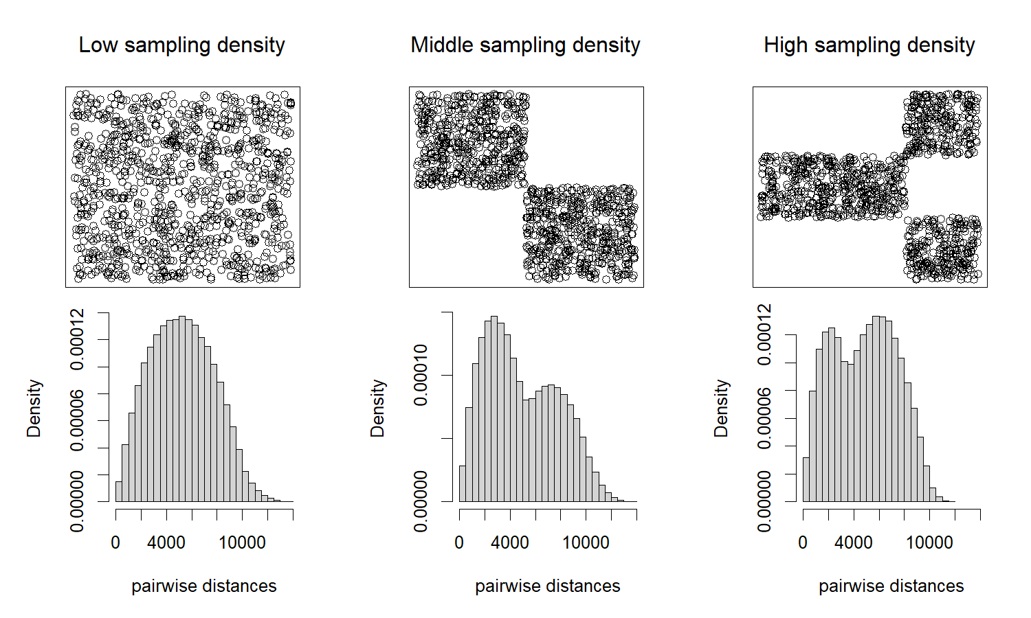
Figure 1: Example for sampling densities and resulting distribution of pairwise distances. Three subsets are sampled from the simulated population with $N=1000$ and either a low, middle or high sampling density. The upper row shows the sample locations on the map $D$ according to the sampling density schemes. The empirical distribution of the pairwise distances is provided below.

3.3 Metaparameters for the empirical semi-variogram

The maximal distance specifies the maximum value up to which pairwise distances are considered within the semi-variogram estimation process. Three values $1.1\cdot h^{*},1.5\cdot h^{*}$ and $2\cdot h^{*}$ are used. The true practical range according to the given semi-variogram model is $h^{*}=415.89$.

The number of lag intervals is chosen to be $10$. Accordingly, the range of pairwise distances from 0 to the maximal distance is divided into 10 equidistant lag intervals. For each interval, a point estimate is calculated based on all point pairs within the lag bin for the empirical semi-variogram.

3.4 Tuning parameters for the filter methods

For the check-based filter approach, the factor $\tau$ scaling the threshold of the test has to be specified. Within the frame of the simulation study, the values $1.1,1.2,1.5,2.0,2.5,3.0$ are applied.

For the quantile-based filter method, the percentage of the quantile threshold $\alpha$ has to be chosen. Values ranging from $0.75$ to $1.0$ with a step length of $0.05$ are put to the test. The value 1.0 equals the case with no filtering and serves as benchmark.

3.5 Conduction of the simulation study and elimination of ill-fitting models

Each scenario is simulated $n_{sim}=3000$ times. Very large or non-positive estimates for at least one of the semi-variogram parameters are an indicator that the algorithm did not converge in the estimation process. Only estimated models fulfilling

$$0<\hat{c_{0}}<1000\;\;\text{and}\;\;0<\hat{\sigma_{0}^{2}}<1000\;\;\text{and}\;\;0<\hat{\phi}<1000$$ (15)

are assumed to have converged and will be included into the evaluation. This leaves $\tilde{n}_{sim}<n_{sim}$ simulation runs to be analyzed. The proportion $\tilde{n}_{sim}/n_{sim}$ will be referred to as the convergence rate in section 4.

3.6 Performance measures

The performance statistics are presented as averages grouped by the sample size, the sampling density, the maximal distance factor and the tuning parameter specification for each filter method. The empirical standard deviation over the parameter estimates of all simulation runs $\eta_{\theta_{j}}=sd(\hat{\theta_{j}})$ for $j=1,2,3$ serves as approximation to the true standard error and benchmark value for our performance evaluation. Its variability is obtained by the Monte Carlo standard error estimator $se_{MC}(\eta_{\theta_{j}})=sd(\hat{\theta_{j}})/\sqrt{2(\tilde{n}_{sim}-1)}$. The performance will be evaluated in terms of the estimates’ standard deviation, bias and mean squared error.

The grouped average estimate $\overline{\widehat{\eta_{\theta_{j}}}}$ according to each grouping parameter is provided along with its grouped average of the corresponding standard deviations $sd(\widehat{\eta_{\theta_{j}}})$. For instance, the grouped average estimate given the grouping factor $N=500$ is obtained by averaging over all estimates for sampling scenarios with $N=500$ and arbitrary specification for the sampling density, maximal distance factor and tuning parameter. The standard deviations of the same scenarios are averaged to obtain the grouped average standard deviation.

The bias is defined as

$$bias(\widehat{\eta_{\theta_{j}}})=\overline{\widehat{\eta_{\theta_{j}}}}-\eta_{\theta_{j}}.$$ (16)

The overall performance is measured in terms of the mean squared error (MSE)

$$MSE(\widehat{\eta_{\theta_{j}}})=sd(\widehat{\eta_{\theta_{j}}})^{2}+bias(\widehat{\eta_{\theta_{j}}})^{2}$$ (17)

taking into account the performance in regards to both, the location of the estimated standard error and the variability described by the squared empirical standard deviation of the estimated standard error estimates.

4 Results

In the following, the simulation study results are described. Compact result tables can be found in the appendix.

4.1 Convergence rate for the estimation of the parameters

The convergence rate $\tilde{n}_{sim}/n_{sim}$ is on grouped average lowest for a sample size of 500 with $51\%$. It increases with increasing sample size leading to $76\%$ for $N=1000$ and $92\%$ for $N=2000$. An increase in the sampling density leads to a slighter increase in the convergence rate ranging from $67\%$ for a low sampling density to $78\%$ in case of middle and $95.9\%$ in case of a high sampling density. Similarly, an increase in the maximal distance factor provides a slighter increase in the convergence rate from $61\%$ for a maximal distance factor of $1.1$ over $75\%$ for a maximal distance factor of $1.5$ to $84\%$ for a maximal distance factor of $2$ (Table 3).

4.2 Performance of generalized bootstrap approach with no filter

Table 1: Generalized bootstrap method with no filter - Performance measure results for the nugget effect $c_{0}$, partial sill $\sigma_{0}^{2}$ and shape parameter $\phi$. Result statistics are rounded to the 2nd decimal point and more for numbers with more than 6 decimals.

semi-variogram parameter	$\eta_{\theta_{i}}$ ($se_{MC}(\eta_{\theta_{i}})$)	$\overline{\widehat{\eta_{\theta_{i}}}}$ ($sd(\widehat{\eta_{\theta_{i}}})$)	$bias(\widehat{\eta_{\theta_{i}}})$	$MSE(\widehat{\eta_{\theta_{i}}})$
$c_{0}$	14.95 (0.0433)	6.64          (4.21)	-8.31	86.75
$\sigma_{0}^{2}$	14.61 (0.0424)	1606.99   (55093.93)	1592.38	$3.04\cdot 10^{9}\;$
$\phi$	166.43 (0.4827)	6035.77 (184498.18)	5869.34	$3.41\cdot 10^{10}$

The standard error estimates calculated with the generalized bootstrap approach with no filter for nugget effect, partial sill and shape parameter averaged with respect to the implemented sampling schemes and metaparameters differ in the observed performance measurements (see Table 1). For nugget effect standard errors, small standard deviation and slightly negative bias is obtained. The corresponding MSE of 86.75 is relatively small. For the partial sill and shape parameter we observe a high variance and high positive bias. This results in a large MSE of more than $3\cdot 10^{9}$ for both parameters.

4.3 Performance of the check filter method

In the following, the effects of the sample size, sampling density, maximal distance and choice of threshold factor on the performance of the standard error estimation with check filtering are presented based on the grouped average outcomes. Tables containing the detailed results of the simulation study results can be found in the appendix (Tables 4, 5, 6).

Effect of sample size: A higher sample size improves all parameters’ standard error estimates. This is indicated by the decreasing MSE as overall performance measure observed for increasing sample sizes.

Effect of sampling density: For $\widehat{\eta_{c_{0}}}$ and $\widehat{\eta_{\phi}}$ all performance measurements indicate very slight improvement with increasing sampling density. For $\widehat{\eta_{\sigma_{0}^{2}}}$ the estimation is relatively worst in case of the middle sampling density, improves little in case of the high sampling density and best when using the small sampling density. It is not clear whether the small differences between low, middle and high sampling density results indicate an effect at all.

Effect of maximal distance: Specifying a higher maximal distance for the model fitting improves the standard error estimation slightly for all semi-variogram parameters. This effect is observed in all performance measurements.

Effect of tuning parameter: Although, the check filter has the expected effect of reducing the variance (or standard deviation $sd(\widehat{\eta_{\theta_{i}}})$ respectively) and the bias of the standard error estimation of all parameters, the effect on the performance and thereby the threshold factor value optimizing the estimation performance is different for each.

The standard error for the nugget effect is estimated best when using the generalized bootstrap approach with no filter. When applying the check filter, a smaller $\tau$ (equivalent to more severe filtering) leads to more underestimated standard error and thereby to a larger MSE. However, the observed effect is very small.

Adding a check filter to the partial sill standard error estimation improves the performance immensely compared to the generalized bootstrap estimation with no filtering. Among the implemented threshold factors, we observe that decreasing $\tau$ leads to better estimation results according to all three performance measures.

Similar to the partial sill, a check filter applied in the shape parameter standard error estimation leads to strongly improved estimator performance compared to the generalized bootstrap approach with no filtering. Among the implemented threshold factors, slight differences in the performance measurements are observed. While most severe filtering with $\tau=1.1$ minimizes the variance in the estimations, simultaneously, the bias is closest to zero for $\tau=3.0$. More severe filtering leads to more negative bias. According to the MSE, $\tau=1.5$ is a suitable compromise.

4.4 Performance of the quantile filter method

The effects of the sample size, sampling density, maximal distance and choice of quantile threshold value on the performance of the standard error estimation with quantile filtering are presented based on the grouped average outcomes. Tables containing the detailed simulation study results can be found in the appendix (Tables 7, 8, 9).

Effect of sample size: Increasing the sample size leads to an improvement of the standard error estimation for all three parameters according to all performance measures.

Effect of sampling density: For $\eta_{c_{0}}$, a slight improvement in the estimation performance is observed when the sampling density is higher. For $\widehat{\eta_{\sigma_{0}^{2}}}$ and $\widehat{\eta_{\phi}}$, a middle to high sampling density leads to better estimator performance compared to a low sampling density with slight preference for the middle density in all performance measures.

Effect of maximal distance: The effect of the maximal distance on the estimation performance shows the same tendencies as the effect of the maximal distance. For $\widehat{\eta_{c_{0}}}$, a slight improvement in the estimation performance is observed when the maximal distance is increased. For $\widehat{\eta_{\sigma_{0}^{2}}}$ and $\widehat{\eta_{\phi}}$, a maximal distance factor of 1.5 or 2.0 leads to better estimator performance compared to a maximal distance factor of 1.1 with slight preference for the 1.5 factor in regards to all performance measures.

Effect of tuning parameter: As expected, more severe filtering by smaller quantile threshold values $\alpha$ decreases variance and bias of the standard error estimator for each parameter. But this has different implications on the performance for each parameter.

For the nugget effect, standard error estimation using the generalized bootstrap without filter leads to slightly less negative bias than applying a filter. Comparison of the MSE as overall performance measure implicates the same: using no filter leads to the best standard error estimation for the nugget effect.

For the partial sill, using a filter improves the standard error estimation by far compared to the approach without filtering. Although the differences in performance are much smaller when comparing the results for the different implemented quantile thresholds, a slight trend toward smaller $\alpha$ values and thereby to more severe filtering within the bootstrap to improve performance according to all performance measures is observed.

For the shape parameter, the addition of the filter in the generalized bootstrap leads to immense improvement within the standard error estimation compared to the no-filter version. Although even the least severe filter with $\alpha=0.95$ leads too a small negative bias, the MSE indicates that more severe sampling improves the standard error estimation in regards to bias and variance considered together.

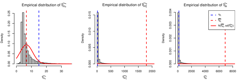
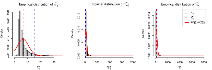
Figure 2: Empirical distribution of standard error estimates obtained with generalized bootstrap without filtering (row 1) and with check filtering with threshold value $3.0$ (row 2). Each histogram is based on all simulation results (all framework conditions). The standard deviation calculated from all simulation estimates $\eta_{\theta_{i}}$ is marked in blue. The average standard error estimate $\overline{\widehat{\eta_{\theta_{i}}}}$ with normal density based on the average standard error estimate and standard deviation of the standard error estimates are provided in red.

5 Discussion

The generalized bootstrap approach of Olea and Pardo-Igúzquiza [7] provides standard error estimates which our simulation study shows to be hugely biased upwards and rather instable as far as the standard error estimator of the partial sill and shape parameter are concerned (see Figure 2). An explanation can be found in the semi-variogram estimation in praxis:

1. The data analyst fits multiple semi-variogram models trying multiple metaparameter values, for instance for the number of bins and maximal distance.

2. The data analyst evaluates by eye how well the semi-variogram model fits the corresponding empirical semi-variogram. The best looking model is chosen for further statistical inference. The other models are discarded.

This procedure contains implicit filter mechanisms. Ill-fitting models and corresponding parameter estimates are thus discarded and we need to introduce an automated filter mechanism within each bootstrap repetition. Therefore, we developed explicit check- and quantile filter rules and tried a range of tuning alternatives within the simulation study. We selected the best alternative based on the simulation results.

The issue of ill-fitting parametric semi-variograms concern also the simulation study itself. For that reason, we implemented the heuristic filter rule stated in sec. 3.5 to identify and exclude generated data that would supposedly be discarded by a practitioner. However this method is imperfect and makes the evaluation of the "true" standard error of the semi-variogram parameters difficult.

5.1 The optimal filter

Compared to the generalized bootstrap approach without filter, all implemented filter extensions reduce the bias upwards and the instability in the standard error estimates. While applying any filter has a negligible negative effect on the performance of the nugget effect’s standard error estimator relative to the true standard error, estimates of standard errors for the partial sill and shape parameters are immensely improved by the procedure.
The check and quantile filter extension are similar in that they exclude bootstrap parameter estimates that are too high. An advantage of the check-based filter approach is the automated comparison of the spatial data variance with the variance estimated according to the semi-variogram model $c_{0}+\sigma_{0}^{2}$. Due to this dependence, the check filter is mainly regulated by the empirical variance induced by the data. The threshold factor provides an option for fine tuning and can be calibrated with the simulation results. The lack of relation between the quantile-based filter and the data context makes tuning of the corresponding tuning parameter $\alpha$ less intuitive.

5.2 Effects of simulation parameters on the standard error estimation

The effects of sample size, sampling density and maximal distance specification on the performance of the standard error estimation observed in the simulation study mirror the effect on parameter estimation of the semi-variogram itself as seen in Sauzet et al. [2]. Because of the empirical nature of the bootstrap approach, adjusting the framework parameters to improve semi-variogram modelling automatically improves the performance of the standard error estimation.

5.3 Recommendations for action

We recommend the generalized bootstrap method with check-based filtering and tuning parameter specification $\tau=3.0$. If controllable, sample size and density are preferably large in order to provide enough point pairs within the lag bins up to the practical range.

6 Case study

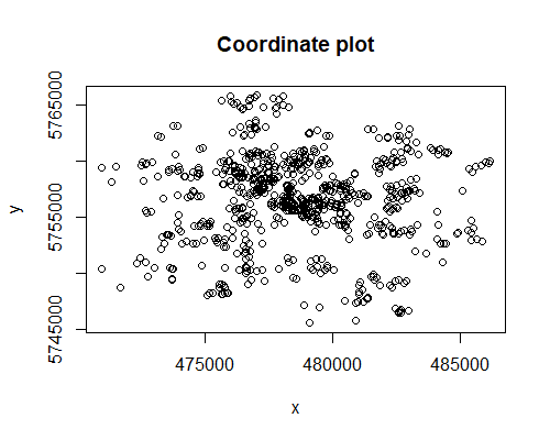
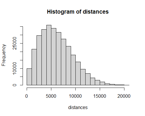
Figure 3: Plot of geo-masked coordinates (left) and a histogram of all pairwise Euclidean distances resulting from the coordinates (right).

The generalized bootstrap with check-based filtering is demonstrated on data obtained from the BaBi birth cohort study [21]. Within the study period from 2013 to 2016 information were gathered about 965 newborn babies and their families including health status attributes and household locations.

Following the same steps as in the work of Sauzet et al. we use geo-masked coordinates of the household locations to model the spatial semi-variance of birthweights [2]. Excluding subjects with incomplete information leaves 783 data points for the modelling procedure. The geo-masked locations of the households and a histogram of the pairwise distances are shown in Figure 3.

Besides the choice of the exponential semi-variogram model form, the maximal distance and number of lag intervals have to be chosen. We fit models with varying metaparameter specifications. The fit is evaluated by visual inspection and comparison of the estimated variance according to the semi-variogram model $\hat{\sigma}^{2}_{model}=\hat{c_{0}}+\hat{\sigma}_{0}^{2}$ with the sample variance $\hat{\sigma}_{sample}^{2}$ by calculating the relative bias as the ratio

$$RB=\frac{\hat{\sigma}^{2}_{model}}{\hat{\sigma}_{sample}^{2}}.$$ (18)

First, we try out a range of maximal distances $(400,500,600,700,800,900,1000)$ and one number of lags $(13)$. By looking at visualizations of the models, we tend to a maximal distance of $800$. The estimated variance is higher by a factor of $2.09\%$ than the sample variance according to the relative bias.

Given the maximal distance of $800$ we try out multiple lag bin numbers $(10,11,12,13,14,15)$. Visually, the models with 10 lags (Model 1) and 13 lags (Model 2) seem to have similarly good fit and provide the two smallest relative biases by a factor of $1.16\%$ and $2.09\%$ out of all alternative models.

We estimate the parameter standard errors using the generalized bootstrap with check-based filtering and tuning parameter $\tau=3.0$. While the parameter estimates for both models are similar, Model 2 provides smaller standard error estimates and is selected as final model (Table 2).

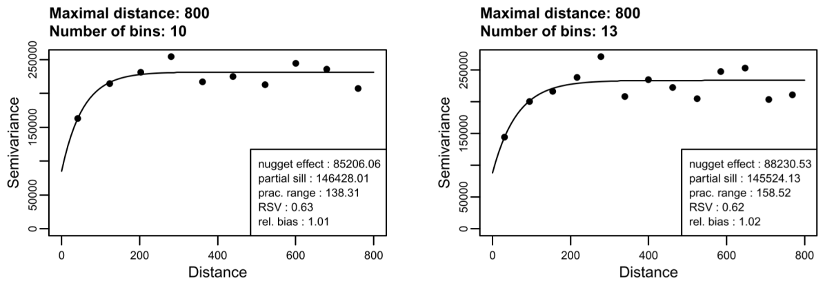
Figure 4: Semi-variogram models fitted to birthweight data with a prespecified maximal distance of 800 and 10 lag intervals (left), as well as, 13 lag intervals (right).

Table 2: Semi-variogram model parameter and standard error estimates for birthweight data. Model 1 refers to the exponential semi-variogram model with a prespecified maximal distance of 800 and 10 lag intervals. Model 2 refers tothe exponential semi-variogram model with a prespecified maximal distance of 800 and 13 lag intervals.

	Model 1		Model 2
	Parameter estimate	Standard error estimate	Parameter estimate	Standard error estimate
$\mathbf{c_{0}}$	85206.06	141638.53	88230.53	145214.64
$\mathbf{\sigma_{0}^{2}}$	146428.01	366958.70	145524.13	338533.10
$\mathbf{\phi}$	54.51	419.08	62.86	337.79

Estimates of semi-variogram parameters have very skewed distributions and the standard deviation cannot be interpreted in the usual sense. Here, the large values are to be understood as how unstable the model is and indicate that the evidence of spatial correlation in the data is rather poor. This follows from the limited number of pairs of observations at small-distances.

7 Conclusion and limits

7.1 Conclusion

Standard errors for the exponential semi-variogram model parameters provide a basis for inference and evaluation of the fitted model that exceeds subjective evaluation by eye. Existing approaches do not work reliably for typical social epidemiological spatial analyses. We developed new approaches to estimate the standard errors of the parameters of an exponential semi-variogram model: The generalized bootstrap method with either check- or quantile-based filtering. Both approaches were presented and evaluated using a simulation study considering multiple framework scenarios varying with regards to sample size, sampling density and maximal distance specifications, as well as multiple tuning alternatives for each filter option. According to the simulation study results, all implemented filter extensions lead to a massive improvement of the standard error estimator compared to the generalized bootstrap without filtering. Another pro argument for the filter extensions is the fact that the implemented filter serves as heuristic rule to approximate the implicit filter mechanism conducted during semi-variogram model fitting in practice. The check filter has a stronger relation to the data variance and is therefore believed to be more intuitive and easier to tune than the quantile filter. Based on the simulation study results and discussed thoughts, we recommend the generalized bootstrap method with check-based filtering and threshold factor $\tau=3.0$ for application.

7.2 Limits

So far, we focused on the exponential semi-variogram with nugget effect since it is of great interest in the study of neighbourhood correlation. However, the generalized bootstrap method with filtering is conceptualized for every kind of parametric semi-variogram model, such as Gaussian, Whittle or Spherical. A simulation study for these parametric model forms has to be conducted, yet.

Acknowledgments

We thank all contributors and authors of the BaBi cohort study [21] for the permission to use the dataset.

Disclosure statement(s) The authors report there are no competing interests to declare.

Data availability statement Data from the BaBi study was used for demonstration purposes. Because of ethical restrictions, the data are available only upon request.

Appendix A Simulation study results

Table 3: Percentage of averaged probable runs grouped by sample size, sample density and maximal distance factor. The number of runs per grouping parameter combination (e.g. sample size of 500, low sample density, maximal distance factor of 1.1) is $n_{sim}=3000$. The number of all executed runs per group is then $27000$ and equals 100%. Parameter estimates are obtained by the WLS approach (sec. 2.2).

grouping parameter	$n_{sim}$	$\tilde{n}_{sim}$	% probable WLS runs
$\varnothing$ by sample size
500	27000	13901	51%
1000	27000	20592	76%
2000	27000	24962	92%
$\varnothing$ by sample density
low	27000	18058	67%
middle	27000	20438	76%
high	27000	20959	78%
$\varnothing$ by maximal distance factor
1.1	27000	16488	61%
1.5	27000	20276	75%
2.0	27000	22691	84%

Table 4: Check Filter Method - Performance measure results for the nugget effect $c_{0}$ grouped by sample size, sample density, maximal distance factor and tuning parameter $\tau$.

semi-variogram parameter	$\eta_{\theta_{i}}$ ($se_{MC}(\eta_{\theta_{i}})$)	$\overline{\widehat{\eta_{\theta_{i}}}}$ ($sd(\widehat{\eta_{\theta_{i}}})$)	$bias(\widehat{\eta_{\theta_{i}}})$	$MSE(\widehat{\eta_{\theta_{i}}})$
$\varnothing$ grouped by sample size
500	19.62 (0.1177)	10.11 (5.6337)	-9.5069	122.1197
1000	15.08 (0.0743)	6.59 (3.2210)	-8.4942	82.5259
2000	8.58 (0.0384)	4.08 (1.0185)	-4.5009	21.2949
$\varnothing$ grouped by sample density
low	16.63 (0.0875)	6.87 (4.6803)	-9.7598	117.1596
middle	14.15 (0.0700)	6.10 (3.8460)	-8.0458	79.5263
high	14.01 (0.0684)	6.17 (3.7961)	-7.8395	75.8688
$\varnothing$ grouped by maximal distance factor
1.1	15.58 (0.0858)	6.22 (4.6159)	-9.3582	108.8821
1.5	14.71 (0.0731)	6.24 (4.0820)	-8.4708	88.4165
2.0	14.36 (0.0674)	6.57 (3.7317)	-7.7848	74.5286
$\varnothing$ grouped by tuning parameter $\tau$
1.1	14.95 (0.0433)	5.86 (3.8942)	-9.0828	97.6615
1.2	14.95 (0.0433)	6.17 (4.0354)	-8.7775	93.3292
1.5	14.95 (0.0433)	6.44 (4.1440)	-8.5123	89.6325
2.0	14.95 (0.0433)	6.54 (4.1768)	-8.4112	88.1942
2.5	14.95 (0.0433)	6.57 (4.1877)	-8.3764	87.7004
3.0	14.95 (0.0433)	6.59 (4.1931)	-8.3590	87.4549

Table 5: Check Filter Method - Performance measure results for the partial sill effect $\sigma^{2}_{0}$ grouped by sample size, sample density, maximal distance factor and tuning parameter $\tau$.

semi-variogram parameter	$\eta_{\theta_{i}}$ ($se_{MC}(\eta_{\theta_{i}})$)	$\overline{\widehat{\eta_{\theta_{i}}}}$ ($sd(\widehat{\eta_{\theta_{i}}})$)	$bias(\widehat{\eta_{\theta_{i}}})$	$MSE(\widehat{\eta_{\theta_{i}}})$
$\varnothing$ grouped by sample size
500	19.68 (0.1180)	30.63 (31.8383)	10.9492	1133.5601
1000	13.76 (0.0678)	26.44 (30.0340)	12.6813	1062.8580
2000	8.63 (0.0386)	23.56 (24.6203)	14.9233	828.8651
$\varnothing$ grouped by sample density
low	16.24 (0.0855)	23.03 (26.6813)	6.7810	757.8730
middle	13.84 (0.0685)	28.43 (29.7273)	14.5837	1096.3960
high	13.7 (0.0669)	26.79 (28.5118)	13.0932	984.3554
$\varnothing$ grouped by maximal distance factor
1.1	16.74 (0.0922)	30.85 (36.1504)	14.1098	1505.9402
1.5	13.86 (0.0688)	26.55 (27.9252)	12.6967	941.0220
2.0	13.14 (0.0617)	22.53 (21.2259)	9.3912	538.7330
$\varnothing$ grouped by tuning parameter $\tau$
1.1	14.61 (0.0424)	19.30 (14.4547)	4.6910	230.9429
1.2	14.61 (0.0424)	21.40 (16.4506)	6.7886	316.7075
1.5	14.61 (0.0424)	25.07 (22.3089)	10.4530	606.9529
2.0	14.61 (0.0424)	28.41 (29.7121)	13.8017	1073.2966
2.5	14.61 (0.0424)	30.65 (35.4179)	16.0411	1511.7454
3.0	14.61 (0.0424)	32.42 (40.2369)	17.8072	1936.1004

Table 6: Check Filter Method - Performance measure results for the shape effect $\phi$ grouped by sample size, sample density, maximal distance factor and tuning parameter $\tau$.

semi-variogram parameter	$\eta_{\theta_{i}}$ ($se_{MC}(\eta_{\theta_{i}})$)	$\overline{\widehat{\eta_{\theta_{i}}}}$ ($sd(\widehat{\eta_{\theta_{i}}})$)	$bias(\widehat{\eta_{\theta_{i}}})$	$MSE(\widehat{\eta_{\theta_{i}}})$
$\varnothing$ grouped by sample size
500	184.79 (1.1083)	123.30 (171.2830)	-61.4882	33118.6714
1000	177.56 (0.8750)	68.28   (94.3200)	-109.2805	20838.4870
2000	144.22 (0.6455)	43.24   (50.1536)	-100.9771	12711.7636
$\varnothing$ grouped by sample density
low	170.98 (0.8997)	76.55 (119.4568)	-94.4307	23187.0799
middle	169.24 (0.8371)	71.42 (110.4234)	-97.8230	21762.6725
high	158.86 (0.7759)	64.77   (98.4035)	-94.0835	18534.9506
$\varnothing$ grouped by maximal distance factor
1.1	183.22 (1.0090)	80.61 (132.6585)	-102.6192	28128.9708
1.5	169.41 (0.8413)	71.47 (105.7821)	-97.9494	20783.9406
2.0	149.34 (0.7010)	62.64   (91.7611)	-86.6964	15936.3747
$\varnothing$ grouped by tuning parameter $\tau$
1.1	166.43 (0.4827)	45.00   (63.9584)	-121.4394	18838.2027
1.2	166.43 (0.4827)	52.15   (69.1959)	-114.2826	17848.5779
1.5	166.43 (0.4827)	65.55   (85.7781)	-100.8865	17535.9610
2.0	166.43 (0.4827)	78.55 (111.1835)	-87.8894	20086.3245
2.5	166.43 (0.4827)	87.65 (133.4778)	-78.7840	24023.2575
3.0	166.43 (0.4827)	94.91 (152.9463)	-71.5295	28509.0593

Table 7: Quantile Filter Method - Performance measure results for the nugget effect $c_{0}$ grouped by sample size, sample density, maximal distance factor and tuning parameter $\alpha$.

semi-variogram parameter	$\eta_{\theta_{i}}$ ($se_{MC}(\eta_{\theta_{i}})$)	$\overline{\widehat{\eta_{\theta_{i}}}}$ ($sd(\widehat{\eta_{\theta_{i}}})$)	$bias(\widehat{\eta_{\theta_{i}}})$	$MSE(\widehat{\eta_{\theta_{i}}})$
$\varnothing$ grouped by sample size
500	19.62 (0.1177)	6.40 (4.9385)	-13.2174	199.0893
1000	15.08 (0.0743)	4.07 (2.7157)	-11.0151	128.7070
2000	8.58 (0.0384)	2.59 (1.1072)	-5.9969	37.1887
$\varnothing$ grouped by sample density
low	16.63 (0.0875)	4.28 (3.7703)	-12.3532	166.8155
middle	14.15 (0.0700)	3.85 (3.0847)	-10.3045	115.6991
high	14.01 (0.0684)	3.89 (3.0748)	-10.1221	111.9110
$\varnothing$ grouped by maximal distance factor
1.1	15.58 (0.0858)	3.92 (3.6811)	-11.6626	149.5658
1.5	14.71 (0.0731)	3.93 (3.2720)	-10.7813	126.9426
2.0	14.36 (0.0674)	4.1 (3.0461)	-10.2524	114.3899
$\varnothing$ grouped by tuning parameter $\alpha$
0.75	14.95 (0.0433)	2.09 (1.7179)	-12.8538	168.1719
0.80	14.95 (0.0433)	2.70 (2.0903)	-12.2452	154.3156
0.85	14.95 (0.0433)	3.36 (2.4935)	-11.5860	140.4520
0.90	14.95 (0.0433)	4.11 (2.9409)	-10.8361	126.0688
0.95	14.95 (0.0433)	5.04 (3.4667)	-9.9039	110.1047
1.00	14.95 (0.0433)	6.64 (4.2123)	-8.3068	86.7460

Table 8: Quantile Filter Method - Performance measure results for the partial sill effect $\sigma^{2}_{0}$ grouped by sample size, sample density, maximal distance factor and tuning parameter $\alpha$.

semi-variogram parameter	$\eta_{\theta_{i}}$ ($se_{MC}(\eta_{\theta_{i}})$)	$\overline{\widehat{\eta_{\theta_{i}}}}$ ($sd(\widehat{\eta_{\theta_{i}}})$)	$bias(\widehat{\eta_{\theta_{i}}})$	$MSE(\widehat{\eta_{\theta_{i}}})$
$\varnothing$ grouped by sample size
500	19.68 (0.1180)	558.20 (25208.56)	538.52	$3.36\cdot 10^{8}$
1000	13.76 (0.0678)	355.86 (28324.53)	342.10	$8.02\cdot 10^{8}$
2000	8.63 (0.0386)	77.29 (13782.64)	68.66	$1.90\cdot 10^{8}$
$\varnothing$ grouped by sample density
low	16.24 (0.0855)	350.68 (27205.76)	334.43	$7.40\cdot 10^{8}$
middle	13.84 (0.0685)	251.10 (17413.02)	237.26	$3.03\cdot 10^{8}$
high	13.7 (0.0669)	264.91 (22420.21)	251.21	$5.03\cdot 10^{8}$
$\varnothing$ grouped by maximal distance factor
1.1	16.74 (0.0922)	564.73 (30973.09)	547.99	$9.60\cdot 10^{8}$
1.5	13.86 (0.0688)	173.29 (13364.20)	159.43	$1.79\cdot 10^{8}$
2.0	13.14 (0.0617)	184.74 (21672.27)	171.59	$4.70\cdot 10^{8}$
$\varnothing$ grouped by tuning parameter $\alpha$
0.75	14.61 (0.0424)	17.72       (16.86)	3.11	293.89
0.80	14.61 (0.0424)	19.18       (19.60)	4.57	404.83
0.85	14.61 (0.0424)	21.03       (23.48)	6.42	592.40
0.90	14.61 (0.0424)	23.69       (29.86)	9.08	974.26
0.95	14.61 (0.0424)	28.65       (44.45)	14.03	2172.62
1.00	14.61 (0.0424)	1606.99 (55093.93)	1592.38	$3.04\cdot 10^{9}$

Table 9: Quantile Filter Method - Performance measure results for the shape effect $\phi$ grouped by sample size, sample density, maximal distance factor and tuning parameter $\alpha$.

semi-variogram parameter	$\eta_{\theta_{i}}$ ($se_{MC}(\eta_{\theta_{i}})$)	$\overline{\widehat{\eta_{\theta_{i}}}}$ ($sd(\widehat{\eta_{\theta_{i}}})$)	$bias(\widehat{\eta_{\theta_{i}}})$	$MSE(\widehat{\eta_{\theta_{i}}})$
$\varnothing$ grouped by sample size
500	184.79 (1.1083)	2467.08 (100233.56)	2282.29	$1.01\cdot 10^{10}$
1000	177.56 (0.875)	1173.72   (92747.11)	996.17	$8.60\cdot 10^{9}$
2000	144.22 (0.6455)	157.78   (28836.16)	13.56	$8.32\cdot 10^{8}$
$\varnothing$ grouped by sample density
low	170.98 (0.8997)	1356.23   (89648.65)	1185.25	$8.04\cdot 10^{9}$
middle	169.24 (0.8371)	859.64   (57975.26)	690.41	$3.36\cdot 10^{9}$
high	158.86 (0.7759)	970.59   (76846.18)	811.74	$5.91\cdot 10^{9}$
$\varnothing$ grouped by maximal distance factor
1.1	183.22 (1.009)	1858.85   (86269.15)	1675.63	$7.45\cdot 10^{9}$
1.5	169.41 (0.8413)	641.66   (48402.07)	472.25	$2.34\cdot 10^{9}$
2.0	149.34 (0.701)	826.04   (85884.05)	676.71	$7.38\cdot 10^{9}$
$\varnothing$ grouped by tuning parameter $\alpha$
0.75	166.43 (0.4827)	38.21         (55.50)	-128.23	19523.01
0.80	166.43 (0.4827)	42.65         (66.53)	-123.79	19749.24
0.85	166.43 (0.4827)	48.53         (82.68)	-117.91	20738.49
0.90	166.43 (0.4827)	57.37       (109.99)	-109.07	23993.38
0.95	166.43 (0.4827)	74.97       (175.01)	-91.46	38990.93
1.00	166.43 (0.4827)	6035.77 (184498.18)	5869.34	$3.41\cdot 10^{10}$

References

- \bibcommenthead
- Bard [1974] Bard, Y.: Nonlinear parameter estimation, p. 170. Academic Press, New York (1974)
- Sauzet et al. [2021] Sauzet, O., Breiding, J.H., Zolitschka, K.A., Breckenkamp, J., Razum, O.: An ego-centred approach for the evaluation of spatial effects on health in urban areas based on parametric semi-variogram models: concept and validation. BMC medical research methodology 21(1), 1–12 (2021)
- Breckenkamp et al. [2021] Breckenkamp, J., Razum, O., Spallek, J., Berger, K., Chaix, B., Sauzet, O.: A method to define the relevant ego-centred spatial scale for the assessment of neighbourhood effects: the example of cardiovascular risk factors. BMC public health 21(1), 1–7 (2021)
- Cressie [1993] Cressie, N.A.C.: Statistics for Spatial Data, Rev. ed. edn. Wiley, New York (1993). https://onlinelibrary.wiley.com/doi/book/10.1002/9781119115151
- Webster and Oliver [2007] Webster, R., Oliver, M.A.: Geostatistics for environmental scientists, 2nd ed. edn. Statistics in practice, p. 119. Wiley, Chichester and Hoboken, NJ (2007). https://doi.org/10.1002/9780470517277
- Pardo-Igúzquiza and Dowd [2001] Pardo-Igúzquiza, E., Dowd, P.: Variance-covariance matrix of the experimental variogram: Assessing variogram uncertainty. Mathematical Geology 33(4), 397–419 (2001) https://doi.org/10.1023/A:1011097228254
- Olea and Pardo-Igúzquiza [2011] Olea, R.A., Pardo-Igúzquiza, E.: Generalized bootstrap method for assessment of uncertainty in semivariogram inference. Mathematical Geosciences 43(2), 203–228 (2011) https://doi.org/10.1007/s11004-010-9269-6
- Saha and Datta [2018] Saha, A., Datta, A.: Brisc: bootstrap for rapid inference on spatial covariances. Stat 7(1), 184 (2018)
- Schabenberger and Gotway [2005] Schabenberger, O., Gotway, C.A.: Statistical Methods for Spatial Data Analysis. Texts in statistical science, p. 488. Chapman and Hall/CRC, Boca Raton [u.a.] (2005)
- Matheron [1963] Matheron, G.: Principles of geostatistics. Economic Geology 58(8), 1246–1266 (1963) https://doi.org/10.2113/gsecongeo.58.8.1246 https://pubs.geoscienceworld.org/economicgeology/article-pdf/58/8/1246/3481854/1246.pdf
- Cressie [1985] Cressie, N.: Fitting variogram models by weighted least squares. Journal of the international Association for mathematical Geology 17(5), 563–586 (1985)
- Pebesma [2004] Pebesma, E.J.: Multivariable geostatistics in s: the gstat package. Computers & geosciences 30(7), 683–691 (2004)
- Pebesma [2014] Pebesma, E.J.: Gstat User’s Manual. Dept. of Physical Geography, Utrecht University, Utrecht, The Netherlands (2014). Dept. of Physical Geography, Utrecht University. https://www.gstat.org/gstat.pdf
- Deutsch and Journel [1998] Deutsch, C.V., Journel, A.G.: V.2 Gaussian-Related Algorithms. GSLIB : geostatistical software library and user’s guide, 2nd ed. edn., pp. 141–149. New York (N.Y.) : Oxford university press, ??? (1998). http://lib.ugent.be/catalog/rug01:000429582
- Shortridge [2008] Shortridge, A.: nscore.R (2008). https://msu.edu/ashton/research/code/nscore.R
- Solow [1985] Solow, A.R.: Bootstrapping correlated data. Journal of the International Association for Mathematical Geology 17(7), 769–775 (1985) https://doi.org/10.1007/BF01031616
- R Core Team [2020] R Core Team: R: A Language and Environment for Statistical Computing. R Foundation for Statistical Computing, Vienna, Austria (2020). R Foundation for Statistical Computing. https://www.R-project.org/
- French [2018] French, J.: SpatialTools: Tools for Spatial Data Analysis. (2018). R package version 1.0.4. https://CRAN.R-project.org/package=SpatialTools
- Dyck et al. [2022] Dyck, J., Sauzet, O., Koslik, J.-O.: EgoCor: Simple Presentation of Estimated Exponential Semi-Variograms. (2022). R package version 1.0.1. https://github.com/julia-dyck/EgoCor
- Dyck et al. [2023] Dyck, J., Sauzet, O., Koslik, J.-O.: EgoCorSim: Functions for Simulation Study. (2023). R package version 0.0.1
- Spallek et al. [2017] Spallek, J., Grosser, A., Höller-Holtrichter, C., Doyle, I.-M., Breckenkamp, J., Razum, O.: Early childhood health in bielefeld, germany (babi study): study protocol of a social-epidemiological birth cohort. BMJ Open 7(8) (2017) https://doi.org/10.1136/bmjopen-2017-018398 https://bmjopen.bmj.com/content/7/8/e018398.full.pdf