Quantum phase diagram of high-pressure hydrogen

The interplay between electron correlation and nuclear quantum effects makes our understanding of elemental hydrogen a formidable challenge. Here, we present the phase diagram of hydrogen and deuterium at low temperatures and high-pressure ($P>$300\text{\,}\mathrm{GPa}$)$ by accounting for highly accurate electronic and nuclear enthalpies. We evaluated internal electronic energies by diffusion quantum Monte Carlo, while nuclear quantum motion and anharmonicity have been included by the stochastic self-consistent harmonic approximation. Our results show that the long-sought atomic metallic hydrogen, predicted to host room-temperature superconductivity, forms at $577(10)\text{\,}\mathrm{GPa}$ ($640(14)\text{\,}\mathrm{GPa}$ in deuterium). Indeed, anharmonicity pushes the stability of this phase towards pressures much larger than previous theoretical estimates or attained experimental values. Before atomization, molecular hydrogen transforms from a conductive phase III to another metallic structure that is still molecular (phase VI) at $422(40)\text{\,}\mathrm{GPa}$ ($442(30)\text{\,}\mathrm{GPa}$ in deuterium). We predict clear-cut signatures in optical spectroscopy and DC conductivity that can be used experimentally to distinguish between the two structural transitions. According to our findings, the experimental evidence of metallic hydrogen has so far been limited to molecular phases.

In 1968, Ashcroft predicted that atomic metallic hydrogen is a room temperature superconductor (?). During the last fifty years, a lot of effort was devised to synthesize atomic hydrogen in laboratory under stable conditions. Nonetheless, the challenge proved more difficult than expected. Solid hydrogen at high pressures exhibits a very rich phase diagram with the presence of five different molecular phases, labeled from I to V (?, ?, ?). Recently, a new phase transition has been observed above $420\text{\,}\mathrm{GPa}$ into a metallic state by infrared (IR) absorption measurements (?), i.e. phase VI. However, Eremets et al. (?) measured the Raman and reflectivity spectra of hydrogen up to $480\text{\,}\mathrm{GPa}$ without incurring in any evidence of a sudden change in the sample. At even larger pressures, Diaz and Silvera (?) claimed to have synthesized the atomic metallic hydrogen from reflectivity measurements at $495\text{\,}\mathrm{GPa}$, with reflectivity data in good agreement with theoretical predictions (?), although the reliability of their observation has been questioned (?, ?). Further uncertainties come from technical difficulties in determining pressure at these extreme conditions, which could lead to a mismatch of up to $80\text{\,}\mathrm{GPa}$ (?), jeopardizing the possibility to reproduce results by independent studies.

The structural characterization of these phases is challenging since both neutron and X-ray diffraction experiments require sample sizes non-compatible with pressures larger than $250\text{\,}\mathrm{GPa}$ (?) in hydrostatic conditions. Numerical ab initio simulations play consequently a crucial role in understanding the phase diagram and can in principle address the following questions: Have atomic metallic hydrogen been synthesized yet? At which pressure do we expect to stabilize it? What is the effect of isotope substitution?

Nevertheless, also ab initio approaches have been plagued so far by severe limitations. Indeed, as hydrogen is the lightest element, its nucleus is subject to huge quantum fluctuations that can largely affect its structural properties. Indeed, nuclear quantum effects have been shown to completely reshape the Born-Oppenheimer (BO) energy landscape in hydrogen-rich materials at high-pressure (?, ?, ?), invalidating the phase diagram obtained with classical simulations. Furthermore, many competing structures differ in enthalpy by less than $1\text{\,}\mathrm{meV}$ per atom in a broad range of pressures (?). This makes the identification of the ground state very sensitive to approximations, like the choice of the exchange-correlation functional in density functional theory (DFT) calculations. To overcome this issue, more sophisticated and accurate theories are required, such as the quantum Monte Carlo (QMC) methods (?). For these reasons, the establishment of theoretical calculations fully accounting for both electron correlation energy and lattice anharmonicity at the same level of accuracy is fundamental to determine the hydrogen phase diagram at such high pressure.

To answer the aforementioned questions, we performed hydrogen phase-diagram calculations at a methodological cutting edge, by combining the highly accurate description of electron correlation, within diffusion quantum Monte Carlo (DMC), and the anharmonic lattice optimization accounting for nuclear quantum effects, within the stochastic self-consistent harmonic approximation (?, ?, ?, ?) (SSCHA). DMC is a well-established framework that provides the most accurate internal energies of solid hydrogen (?, ?, ?, ?). Here, it has been coupled to SSCHA in a seamless fashion with the aim of including both electronic and nuclear contributions in a non-perturbative way. Indeed, SSCHA can outperform other approximations to compute anharmonic phase diagrams in hydrogen (?, ?, ?) thanks to its variational nature in determining free energy differences and its ability to relax atomic positions and lattice vectors. In our approach, SSCHA provides both vibrational energies and average nuclear positions (centroids), calculated from nuclear quantum fluctuations developing on the top of a DFT-BLYP (?) energy landscape. The resulting centroids crystal structure is used to compute DMC electronic internal energies, that are combined with the SSCHA zero-point energies of the anharmonic lattice.

We modeled phase III as the monoclinic C2/c-24 structure (?), which is the best representative of this phase (Fig. 1a). Indeed, not only is it the most stable in its pressure range, but also it reproduces optical transmission and reflectivity, Raman and IR experimental data (?).

Besides C2/c-24, we took into account the Cmca-12 crystalline symmetry (Fig. 1b), a new hexagonal structure with P62/c-24 symmetry (Fig. 1c), and the Cmca-4 structure (Fig. 1d) as the most promising molecular geometries for phase VI. Cmca-12 has firstly been suggested by Pickard and Needs as an alternative candidate for phase III (?), and more recently proposed as phase VI (?). Cmca-4 (?) is the ground state in the harmonic DFT phase diagram with common functionals (PBE and BLYP) over a large pressure range, but considerably disfavored by the most accurate QMC internal energies (?, ?). We discovered the new P62/c-24 structure by relaxing the symmetry constraint on the C2/c-24 with quantum anharmonic fluctuations above $320\text{\,}\mathrm{GPa}$ at the DFT-BLYP level of theory. It is made of graphene-like sheets alternating with molecular layers, conferring to the phase similar optical properties to graphite. It is a saddle-point of the BO energy landscape, stabilized by quantum fluctuations (see Supplementary Materials (SM)). However, it turns out that also this crystalline symmetry is disfavored by the QMC energies.

Finally, we simulated the atomic phase I4/amd-2, also named Cs-IV (?) (Fig. 1e). According to DFT, it is the most stable atomic symmetry beyond the molecular phases, and it is the one where room-temperature superconductivity has been predicted (?). In Figure 1, we report the centroid positions of these structures at $650\text{\,}\mathrm{GPa}$ with a visualization of the amplitude of quantum fluctuations.

Figure 1: Structures considered for the low-temperature high-pressure phase diagram of hydrogen. Colored balls are the average centroid positions, sticks represent the H2 molecules, the cloud of smaller gray balls is a set of 250 configurations that sample the quantum probability distribution at $0\text{\,}\mathrm{K}$. All structures, apart from the atomic one, are made of layers, of which we report only one. P62/c-24 is made of alternating layers, one with atoms arranged in a honeycomb lattice (panel b), the other with molecular H2 in a C2/c-24 arrangement (not reported here).

Figure 2: Phase diagram of hydrogen (H: panel a) and deuterium (D: panel b) at $T=$0\text{\,}\mathrm{K}$$. On the top we report the phase diagram obtained by neglecting nuclear zero-point energy (static lattice) and with the harmonic zero-point energy. For the final anharmonic phase diagram we explicitly report the enthalpies of different phase with respect to phase III (C2/c-24). The most stable structure is the lowest in enthalpy at a given pressure. Enthalpies are evaluated at the DMC level. Hydrogen transforms from phase-III (C2/c-24) to phase-VI (Cmca-12) at $422(40)\text{\,}\mathrm{GPa}$ ($442(30)\text{\,}\mathrm{GPa}$ for D), and then to the atomic superconductive phase (Cs-IV) at $577(10)\text{\,}\mathrm{GPa}$ ($640(14)\text{\,}\mathrm{GPa}$ for D). Anharmonicity strongly affects the transition pressures and qualitatively affects the phase diagram of hydrogen. Stochastic errors (black bars) are linearly propagated from DMC and SSCHA errors in total energy to pressure. Systematic errors (red bars) are estimated by changing the reference structure for DMC calculation (see SM for more details).

We present the complete phase diagram for hydrogen (H) and deuterium (D) in Figs. 2(a) and 2(b), respectively. On the top of Figure 2, we report also the phase diagram computed by neglecting the nuclear zero-point motion (static lattice), and the one with the harmonic zero-point energy.

Hydrogen transforms into the atomic metal at $577(15)\text{\,}\mathrm{GPa}$, much above the pressure predicted neglecting anharmonicity. The isotope shift of this transition is one of the biggest ever reported, as deuterium transits into its atomic metallic state at $640(14)\text{\,}\mathrm{GPa}$. Anharmonicity modifies the structure of all molecular phases, stretching the molecular bonds and softening the H2 molecular vibrations by about $1000\text{\,}{\mathrm{cm}}^{-1}$ (?). Thus, the relaxation of anharmonic energy strongly favors molecular phases.

Even though the anharmonic contributions significantly impact the energy difference between molecular and atomic phases, the latter turns out not to be as harmonic as suggested previously (?). Indeed, we found that Cs-IV exhibits a prominent anharmonicity in the cell shape. The only free parameter of the Cs-IV structure is the $c/a$ ratio of the tetragonal lattice. The anharmonicity increases the $c/a$ ratio by about 0.12, independently of the pressure and the level of the electronic theory employed. A recent path integral molecular dynamics calculation also showed a nontrivial anharmonicity in the Cs-IV phase (?), in agreement with us. The correct simulation of the $c/a$ structural parameter has relevant consequences on the superconducting properties: by varying the $c/a$ at a fixed volume, the Cs-IV undergoes a Lifshitz transition that enhances the density of states (DOS) at the Fermi level. Quantum anharmonic fluctuations shift $c/a$ away from the Lifshitz transition, preventing the enhancement of the superconducting critical temperature in the range of pressure where this phase is stable (see SM).

Before becoming an atomic metal, hydrogen undergoes another phase transition between two molecular phases (III$\rightarrow$ VI). This transition occurs at $422(40)\text{\,}\mathrm{GPa}$ for H ($442(30)\text{\,}\mathrm{GPa}$ for D), in agreement with the experimental results of Loubeyre et al. (?). The experimental marker of this phase transition is a sudden drop of the transmittance in the near IR region, ascribed to the closure of the direct bandgap in correspondence to a structural rearrangement. However, other experiments exploring the same pressure range observed the sample under visible light without spotting any trace of phase transition (?, ?). To investigate this situation, we computed the optical properties in the near IR and visible range for phase III (C2/c-24), and for the structure we predict to be stable above $422\text{\,}\mathrm{GPa}$, namely Cmca-12. Our calculations account for electron-phonon interaction non-perturbatively. The electronic bands are computed within the modified Becke-Jonson meta-GGA (?), which shares a similar accuracy with hybrid functionals and self-consistent GW calculations, by following the same methodology discussed in  (?). We find that the Cmca-12 structure does not transmit light in the IR around the transition pressure, in contrast with phase III (C2/c-24), as shown in Figure 3. Our data explain the drop in IR transmittance observed in the experiment (?) and, thus, support the assignment of phase VI to the Cmca-12 symmetry. Moreover, both phase III and VI display an almost identical low reflectivity in the visible window of 1.8-$3.2\text{\,}\mathrm{eV}$ (Figure 4), so they are almost indistinguishable under visible light. This explains why experiments that explored the required pressure did not observe the phase transition (?, ?). We also predict a resistance drop at the phase transition, associated with an increase of the electronic DOS at the Fermi level. Conductivity measurements on hydrogen (?) stop just before the transition pressure. The sudden rise in conductivity is an independent feature that can unambiguously prove the transition to phase VI. Our results differ from a previous theoretical work (?), which adopted a different approximation, where optical electron-hole excitations involving phonons outside the center of the Brillouin zone are not included. Interestingly, Cmca-12 is never the ground state of hydrogen with harmonic zero-point energy, and it is stabilized by anharmonicity.

Figure 3: Simulation of transmittance (upper panels) and the real part of optical conductivity (lower panels) at various pressures, comparing phase III (C2/c-24, blue solid lines) with phase VI (Cmca-12, violet dashed lines). The rainbow colors match their respective energy in the visible spectrum. The arrows highlight differences in the optical properties between the two phases. We observe the transmittance of phase VI dropping down at lower energies than phase III. This phase is already completely opaque at $355\text{\,}\mathrm{GPa}$. Also, DC conductivity is higher in phase VI than phase III. The increase of conductivity around zero energy is the Drude peak and it is a signature of the indirect band gap closure (metallicity). Reflectivity and electronic density of states are reported in SM (Figure 18).

In Figure 4, we report the reflectivity data for the phases III, VI and the atomic one as pressure increases. At each pressure, we show a photo-realistic render of high-pressure solid hydrogen sample in vacuum, simulated by solving the Fresnel equation as implemented in the Mitsuba2 software (?). Phase VI becomes gradually more reflective upon increasing pressure, until it transforms into the atomic Cs-IV at about $577\text{\,}\mathrm{GPa}$, where it becomes shiny, reflecting almost 80 % of the visible light. Despite being significantly attenuated by vibrational disorder, the sudden rise of reflectivity in the visible light is a key signature of the molecular-to-atomic transition. Together with reflectivity, also the static conductivity gradually increases upon loading pressure and jumps to higher value at the transition to the atomic Cs-IV phase (see SM). In contrast to phase VI, the atomic phase shows no significant variation of reflectivity and conductivity with pressure. Interestingly, the quantum nuclear fluctuations have an opposite effect on molecular phases, where they enhance reflectivity, than on the atomic phase, in which the reflectivity is strongly suppressed. The suppression of reflectivity in the atomic phase was already found in other works (?, ?).

Figure 4: Reflectivity (upper panels) and photo-realistic render (lower panels) of high-pressure metallic hydrogen. At the transition between phase III to phase VI there is no visible jump in the reflectivity under visible light and the metal appears almost black. As we increase the pressure, the reflectivity gradually increases until we reach the transition to the atomic phase, where we have a significant jump and the material appears shiny (bottom-right panel). In the top-right panel, we also report the reflectivity obtained without electron-phonon (el-ph) coupling (i.e. a standard static calculation). Interestingly, in molecular phases, the electron-phonon coupling enhances the reflectivity by increasing the DOS at the Fermi level, while, for atomic hydrogen, electron-phonon suppresses it. The data are calculated at the same volume for all phases. For the Cs-IV phase, the corresponding pressure is about $40\text{\,}\mathrm{GPa}$ lower than the one reported in the title (which is approximately the same for C2/c-24 and Cmca-12). The photo-realistic render of the high-pressure hydrogen in vacuum is made by feeding the Mitsuba2 (?) software with the complex refractive index of hydrogen and introducing a texture to simulate both a rough and a smooth appearance, following the methodology discussed in (?).

In conclusion, the hydrogen phase diagram based on both highly accurate electronic internal energies computed by QMC and anharmonic nuclear quantum fluctuations provided by SSCHA, confirms that hydrogen undergoes a first-order phase transition from a conductive phase III (molecular C2/c-24) to metallic phase VI (molecular Cmca-12) at $422(40)\text{\,}\mathrm{GPa}$, in accordance with experiments (?). We predict the transition towards atomic metallic hydrogen to occur at about $577\text{\,}\mathrm{GPa}$, a much larger pressure than those reached so far by experiments (?). Our results indicate that the synthesis of atomic hydrogen has still to be fulfilled.

Supplementary materials

Details on the Phase Diagram calculation and the role of anharmonicity and electronic correlations

In this Section, we describe in details how the phase diagram is computed, and discuss how it changes when we adopt a different electronic theory - density functional theory (DFT) versus diffusion quantum Monte Carlo (DMC) - with and without anharmonicity.

We relaxed each structure by including quantum fluctuations and anharmonicity through the stochastic self-consistent harmonic approximation (SSCHA), optimizing the auxiliary force constants, centroid positions, and lattice vectors within the constraints of the symmetry group, at roughly every 100 GPa (from $250\text{\,}\mathrm{GPa}$ to $650\text{\,}\mathrm{GPa}$). In the SSCHA calculations, we employed the DFT framework with the BLYP (?) exchange-correlation functional to account for electronic energy and determine the Born-Oppenheimer (BO) potential energy surface. BLYP is one of the most accurate DFT functionals for phase-diagram calculations of high-pressure hydrogen, outperforming more refined techniques such as hybrid DFT (?, ?). The full anharmonic energy is obtained within DFT, by fitting with a parabola the difference between the BO energy and the SSCHA total energy at fixed volume for each phase. Also the anharmonic stress tensor is employed in the fit to increase accuracy. We then add to the static BO energy-versus-volume curves, computed in DFT every $5\text{\,}\mathrm{GPa}$, the quantum anharmonic lattice vibrational contribution at the corresponding volume calculated from the fit. We finally perform the Legendre transform to get the enthalpy-vs-pressure curves and the resulting phase diagram.

The static phase diagram simulated within DFT-BLYP is reported in Figure 5, while in Figure 6 we show the DFT-BLYP phase diagram with harmonic zero-point energy . We included the harmonic contributions only for the most relevant phases: C2/c-24, Cmca-12 and Cs-IV. The harmonic zero-point energy leaves almost unchanged the pressure of the C2/c-24 to Cmca-12 transition (phase III to VI), while it substantially shifts the atomic transition down to pressures even lower than the Cmca-12. The results of the anharmonic phase diagram of both hydrogen (${}^{1}\text{H}$ protium or H) and deuterium (${}^{2}\text{H}$ or D) computed by DFT-BLYP and SSCHA are reported in Figure 7. It shows that anharmonicity strongly favors the molecular phases over the atomic one, shifting back the atomic transition to higher pressures. Between Cmca-12 and C2/c-24, anharmonicity favors the Cmca-12 crystal symmetry, moving the III-to-VI phase transition down by about $150\text{\,}\mathrm{GPa}$. In this case, phase VI candidates P62/c-24, Cmca-12 and Cmca-4 are almost degenerate up to $400\text{\,}\mathrm{GPa}$, where the Cmca-4 starts dominating over the other molecular phases.

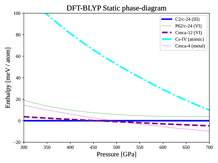
Figure 5: DFT-BLYP static enthalpies (static lattice) of high-pressure hydrogen.

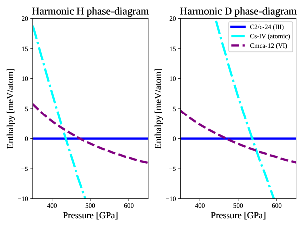
Figure 6: DFT-BLYP enthalpies including nuclear zero-point energy within the harmonic approximation for hydrogen and deuterium, shown on the left and right side, respectively.

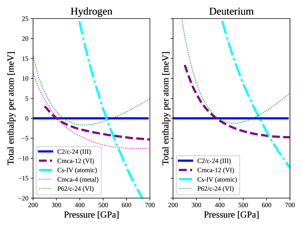
Figure 7: As in Fig. 6, but for the DFT-BLYP enthalpies including quantum anharmonic effects.

Apart from Cmca-4, the DFT-BLYP phase diagram is in qualitative agreement if compared to the one including the electron correlation treated at the quantum Monte Carlo (QMC) level.

Thanks to extensive DMC calculations performed at fixed structures for several phases and volumes, we have been able to correct the DFT-BLYP internal energies, and add the contribution coming from a nearly exact treatment of electron correlation on the top of the static, harmonic and quantum anharmonic phase diagrams previously computed at the DFT-BLYP level. DMC corrections are added on the total energy-versus-volume curves of the corresponding DFT (and DFT+SSCHA) calculations. As in the DFT case, the enthalpy-versus-pressure curves are then obtained by Legendre transform.

For the sake of completeness, we report the static DMC-corrected phase-diagram in Figure 8, the DMC-corrected enthalpies accounting for the nuclear zero-point energy within the harmonic approximation (Figure 9) and the full anharmonic enthalpies with DMC corrections (Figure 10). The latter data provide the final phase diagram reported in the main text.

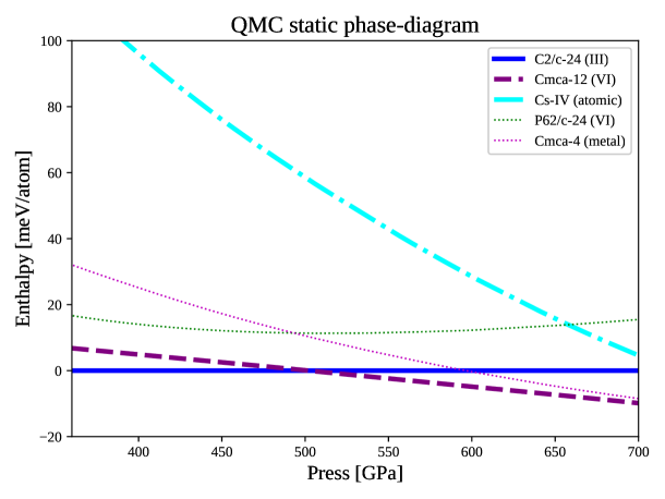
Figure 8: Diffusion QMC static enthalpies (static lattic) of high-pressure hydrogen. Based on these enthalpies, we draw the static-nuclei phase diagram reported in the main text (Figure 2).

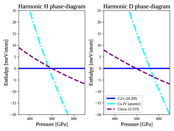
Figure 9: Diffusion QMC enthalpies including nuclear zero-point energy within the harmonic approximation for hydrogen (left panel) and deuterium (right panel). Based on these enthalpies, we draw the harmonic phase diagram reported in the main text (Figure 2). The harmonic zero-point energies are calculated at the DFT-BLYP level and then added to the DMC energies.

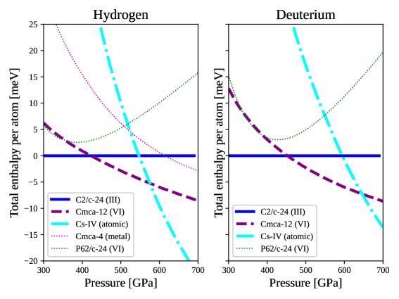
Figure 10: Diffusion QMC enthalpies, including quantum anharmonic effects for hydrogen and deuterium, shown on the left and right side, respectively. Nuclear quantum effects are added based on SSCHA calculations performed at the DFT-BLYP level. The corresponding phase diagram is reported in the main text (Figure 2).

The P62/c-24 symmetry

Among other known structures, we also simulated the new P62/c-24 symmetry we discovered through the relaxation of phase III (C2/c-24) at the anharmonic level within DFT-BLYP.

In particular, phase III becomes unstable at DFT-BLYP level after $310\text{\,}\mathrm{GPa}$, when the free energy curvature becomes negative around an IR-active nuclear vibration at $\Gamma$. In Figure 11 we report the simulation of the C2/c-24 free energy Hessian as a function of pressure along with the unstable nuclear vibration. The free energy Hessian at the SSCHA level is computed with the full expression discussed in Ref. (?), including non perturbatively both three- and four-phonon scattering vertices. Interestingly, this is a very peculiar case where the four-phonon scattering is fundamental to have a correct result, even at a qualitative level, as the C2/c-24 is unstable at all pressures if only three-phonon scattering processes are accounted for.

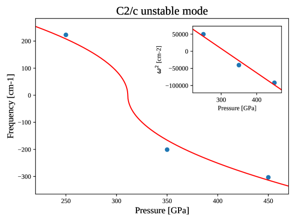
Figure 11: Frequency of the eigenvalue of the free energy Hessian along the unstable nuclear vibration, obtained with DFT-BLYP. On the negative axis we report imaginary values. Inset: the square of the frequency, which correspond to the free energy curvature. A negative value indicates an instability.

The unstable mode breaks the C2/c symmetry in a Cc group with just two symmetry operations and 24 atoms in the unit cell. We performed the full anharmonic relaxation of the new phase. The monoclinic cell becomes hexagonal, and two layers out of four in the primitive cell transform in perfectly graphene-like sheets, with alternated stacking. The other two layers keep their molecular feature, and the H2 molecule reduces its bond length with respect to the C2/c geometry. The transformation of the graphene-like layer is reported in Figure 1b. The symmetry group of the new structure is P62/c, as identified through both ISOTROPY (?) and spglib (?) software. This phase is strongly unstable at harmonic level (it has four degenerate imaginary frequencies at $\Gamma$ above $2000\text{$\mathrm{i}$}\text{\,}{\mathrm{cm}}^{-1}$) but it is stabilized by anharmonicity. As far as we know, this is the first example of a new structure discovered by a full quantum relaxation of nuclear position. This is only possible thanks to the simultaneous relaxation of auxiliary force constants, centroids, and lattice vectors.

When more accurate DMC calculations are employed to evaluate its energy, this phase becomes unfavoured. Therefore, the instability of C2/c-24 towards P62/c is an artifact of the DFT-BLYP functional.

The atomic phase

In the atomic phase, the only free parameter is the c/a ratio of the primitive lattice vectors. In the following, we will then present its main properties as a function of the c/a value.

The structure is stable at the static level, as it has a well-defined minimum. However, suppose we compute phonons at the harmonic level, and use the phonon dispersion to include the kinetic energy of ions due to the quantum zero-point motion. In that case, the total energy decreases with the c/a ratio until imaginary frequencies appear before the minimum is reached, and the system becomes unstable (see Fig. 12). The Cs-IV atomic phase is, therefore, unstable within the quasi-harmonic approximation. The SSCHA fixes this instability: the c/a increases only by about 0.2 compared to the static value. This effect is, however, strongly size-dependent, and its value becomes even smaller (c/a $\approx$ 0.12) when larger cells of 128 atoms are considered, by strengthening the outcome of our analysis.

We computed the free energy Hessian at the SSCHA-relaxed c/a value, and it is stable by a significant amount, shifting the higher energy modes down only by about $250\text{\,}{\mathrm{cm}}^{-1}$. Therefore, even if the structure itself is not so anharmonic, the stability of the structure is met only within a complete anharmonic calculation.

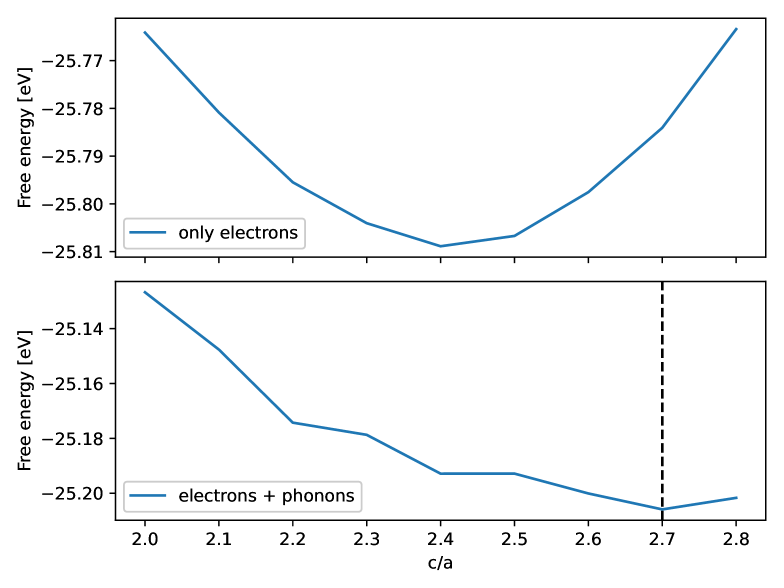
Figure 12: Free energy with static lattice (upper panel) and with harmonic lattice vibrations (lower panel) as a function of c/a. These quantities are computed with the BLYP functional at the volume of $$1.067\text{\,}\mathrm{\SIUnitSymbolAngstrom}$^{3}$ per atom. The vertical dashed line indicates the c/a value where imaginary phonons appear.

It turns out that the c/a equilibrium value is strongly functional dependent. Nevertheless, by running a SSCHA simulation either with BLYP or with PBE, we verified that the effect of the SSCHA on the c/a parameter is additive on the functional used and, thus, the shift with respect to the static equilibrium value is rather functional independent.

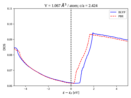
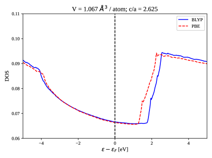
Figure 13: Electronic DOS for c/a values corresponding to BLYP static equilibrium geometry (left panel) and to BLYP equilibrium geometry including also nuclear fluctuations (right panel). The DOS increases when increasing c/a. However, we get further away from the Lifshitz transition for larger c/a values, and this happens for both BLYP (blue lines) and PBE (red lines) functionals.

Interestingly, the atomic phase is in the proximity of a Lifshitz transition, signaled by a sudden jump of the DOS, which is indeed located very close to the Fermi level ($\epsilon_{F}$). This is reported in Figure 13. In particular, although the DOS at $\epsilon_{F}$ steadily increases with c/a, the Lifshitz transition gets further away from $\epsilon_{F}$. The PBE and BLYP functionals predict the same electronic DOS at $\epsilon_{F}$ but slightly different locations for the Lifshitz transition, whose energy is systematically closer to the Fermi level in PBE. The same behavior is found also for the other volumes studied for the atomic phase, as reported in Figure 14. Only at the largest volume taken into account, i.e. V=1.259 ų/atom, the PBE functional triggers the Lifshitz transition, as shown in the bottom-left panel of Figure 14. However, the c/a value reported there corresponds to the BLYP equilibrium geometry of the static lattice. The PBE equilibrium geometry has a larger c/a value, which pushes the Lifshitz transition energy above the Fermi level.

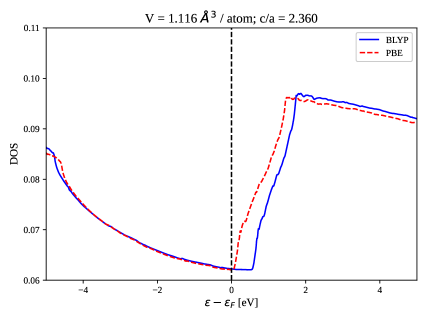
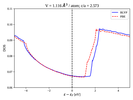
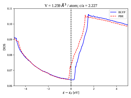
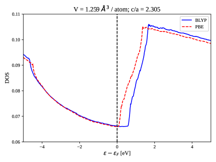
Figure 14: DOS plotted for different volumes and c/a values corresponding to the BLYP static equilibrium geometry (left-hand side), and the BLYP equilibrium geometry with nuclear fluctuations (right-hand side). For these geometries, the DOS is computed with both BLYP (blue lines) and PBE (red lines) functionals.

There is a strong linear correlation between the energy location of the Lifshitz transition and the c/a value, as revealed by plotting the distance of the Lifshitz transition energy from $\epsilon_{F}$ as a function of c/a for all volumes and functionals taken into account (Figure 15). This correlation allows us to estimate the exact c/a value at which the Lifshitz transition occurs for each volume, as obtained by fitting the results in Figure 15 and extrapolating the Lifshitz transition energy to $\epsilon_{F}$ (Figure 16).

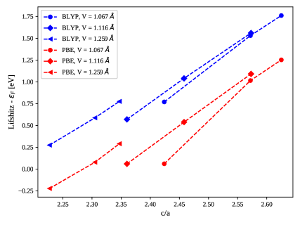
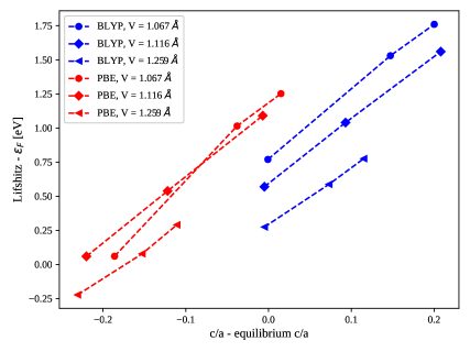
Figure 15: Distance of the Lifshitz transition from the Fermi level. In the left panel, this is plotted as a function of c/a. On the right panel, the origin of the c/a axis is set to the equilibrium value of c/a for each volume and functional. The abscissa at which the curves cross the $y=0$ line is the c/a value when the system undergoes the Lifshitz transition. This is neither volume nor functional universal.

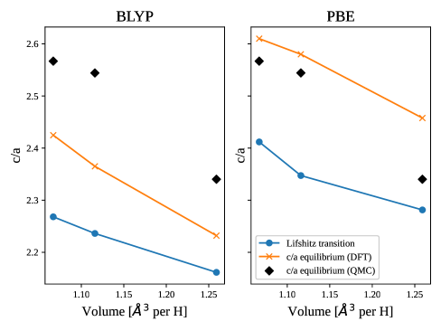
Figure 16: The c/a value at which the Lifshitz transition occurs, causing a sudden increase of the electronic DOS at the Fermi level. We compare the Lifshitz transition with the equilibrium c/a value as yielded by BLYP, PBE, and DMC. Quantum fluctuations move the equilibrium c/a ratio by about 0.1-0.2 towards larger values, independently on the choice of the DFT functional, driving the system away from the transition.

Care must be taken in evaluating the distance of the Lifshitz transition energy from the Fermi level. Indeed, the Fermi level determination could be affected by the choice of the smearing parameter. In our analysis, we employed the so-called "cold" smearing (aka the Marzari-Vanderbilt scheme). We repeated the calculation for three volumes by using the Gaussian smearing and the Fermi-Dirac smearing, and compared their outcome for the Fermi energy determination. It turns out that the difference in the Fermi level is at most $20\text{\,}\mathrm{meV}$. The data are reported in Table 1. This Fermi energy uncertainty converts into an error on the c/a value for the Lifshitz transition of 0.008, much smaller than the variations plotted in Fig. 16.

Volume per H	Marzari-Vanderbilt	Gaussian	Fermi-Dirac
$1.067\text{\,}\mathrm{\SIUnitSymbolAngstrom}^{3}$	$17.115\text{\,}\mathrm{eV}$	$17.161\text{\,}\mathrm{eV}$	$17.156\text{\,}\mathrm{eV}$
$1.116\text{\,}\mathrm{\SIUnitSymbolAngstrom}^{3}$	$16.403\text{\,}\mathrm{eV}$	$16.401\text{\,}\mathrm{eV}$	$16.387\text{\,}\mathrm{eV}$
$1.259\text{\,}\mathrm{\SIUnitSymbolAngstrom}^{3}$	$14.394\text{\,}\mathrm{eV}$	$14.402\text{\,}\mathrm{eV}$	$14.371\text{\,}\mathrm{eV}$

Table 1: Fermi level computed with different smearing schemes and volumes for the atomic Cs-IV phase. The electronic temperature is $0.03\text{\,}\mathrm{Ry}$ and a $48\times 48\times 48$ grid has been used as a k-mesh. The error on the Fermi-level that comes from the choice of the smearing scheme is lower than $0.03\text{\,}\mathrm{eV}$.

The knowledge of the actual volume dependence of the c/a equilibrium value is of paramount importance, because this could potentially have a strong impact on the electronic properties of the atomic metallic phase of hydrogen. Indeed, the sudden increase of the DOS yielded by the Lifshitz transition could affect the superconducting critical temperature. This is a fascinating scenario whose chance of occurrence needs to be addressed by a more accurate method such as QMC. With the aim of determining the exact c/a equilibrium value, we studied the c/a energy curve of BLYP, PBE, and LDA functionals, and compared them with reference results obtained by DMC calculations (Figure 17).

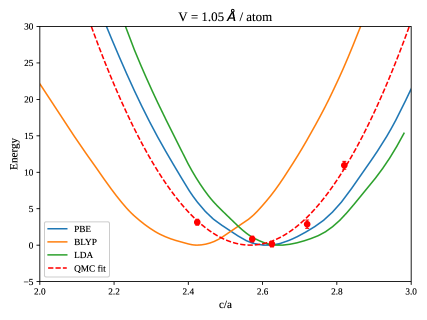
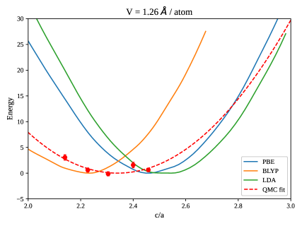
Figure 17: Energy profile as a function of the c/a parameter for different volumes and electronic theories. Three of the c/a points taken in the DMC calculations are the static equilibrium value in BLYP, the SSCHA equilibrium value for deuterium and the one for protium.

From the comparison with the DMC results, one can notice that the BLYP robustness in providing accurate equilibrium geometry deteriorates at small volumes, corresponding to pressures above 560 GPa. The PBE curves show instead the opposite behavior, as they become more and more accurate as the volume shrinks. For the smallest volumes, the PBE results are the most accurate. Therefore, by looking at the right panel of Fig. 16, which reports the PBE equilibrium c/a values compared with the critical c/a values for the Lifshitz transition, we can safely disregard the occurrence of this transition in the pressure range where the atomic metallic phase becomes favorable. Indeed, nuclear quantum effects move the atomic phase further away from the transition.

Optical properties

We report here additional information regarding the optical properties of phase III, phase VI and the atomic one.

To complete the analysis presented in the main text about the comparison between phase III and VI, in Figure 18 we show the electronic density of states (DOS) and the reflectivity of both phases. As mentioned in the main text, phases III and VI are almost indistinguishable from reflectivity measurements in the visible range, but they present differences in the IR frequency range, where reflectivity is enhanced in phase VI. Also, the DOS at the Fermi level of phase VI is higher, resulting in a better DC conductivity of this phase, as reported in Figure 3 of the main text.

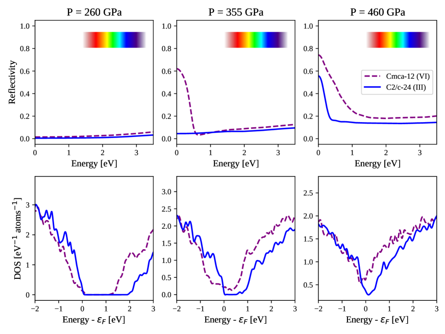
Figure 18: Reflectivity (upper row) and DOS (lower row) of phase III (C2/c-24) and phase VI (Cmca-12) at different pressures.

To compute the optical properties of phase III and VI, we used supercells containing 324 atoms, where phonons are accounted for as static disorder (adiabatic approximation). We evaluated the refractive index and the transmitted light through a $1.5\text{\,}\mathrm{\SIUnitSymbolMicro m}$ thick sample. This is the typical thickness of experimental samples at the target pressures. To avoid the systematic underestimation of the empty bands energy in the DFT calculation, we employed the modified Becke-Johnson meta-GGA exchange-correlation functional (?), which is known to perform as well as more established (and more computationally expensive) methods like the HSE06 hybrid functional or the GW calculations (?). All the calculations details, the equations employed and software used are the same as those discussed in the Methods Section of Ref.  (?).

As far as the comparison between phase IV and the atomic phase is concerned, we complement the data reported in the main text by including the optical conductivity (real and imaginary part) computed for the Cmca-12 and Cs-IV between 460 GPa and 660 GPa in Figure 19.

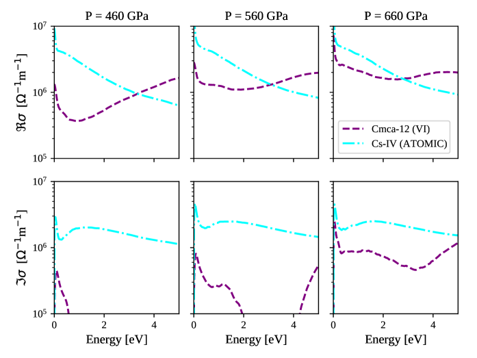
Figure 19: Real and imaginary part of the conductivity of Cmca-12 and Cs-IV phases.

As mentioned in the paper, our results on the optical properties are at variance with the ones of Ref.  (?). This could be explained by the different approach used. Indeed, in Ref.  (?) the authors computed the optical properties on a smaller cell of 96 atoms and measured the optical gap by accounting for electron-hole pair excitations at the same point in the Brillouin zone of the 12-atom cell unfolded bands. In this way, scattering processes involving phonon momenta $\textbf{q}\neq\Gamma$ are not included, where the excited electron-hole pair has a non-zero total momentum. In ordinary materials like silicon, these effects contribute as a small perturbation. However, this is not the case of hydrogen, where the electron-phonon interaction shifts the bands by $2\text{\,}\mathrm{eV}$.

We carried out a thorough study of the convergence of the Cs-IV reflectivity with respect to the number of $\mathbf{k}$-points, the smearing (Figure 20), and the electronic temperature (Figure 21). The reflectivity shown in the main text has been obtained by employing a 729 $\mathbf{k}$-mesh with a smearing of $0.05\text{\,}\mathrm{eV}$. The reflectivity depends weakly on the electronic temperature when its value is lower than the smearing. Thus, at $300\text{\,}\mathrm{K}$, the temperature used in our analysis, the reflectivity is fully converged in its temperature dependence.

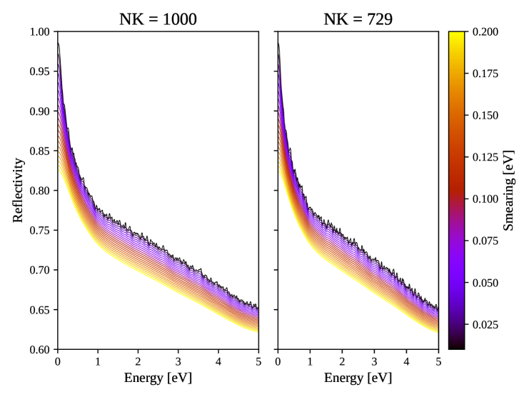
Figure 20: Convergence of the reflectivity as a function of smearing and number of k-points in the Cs-IV phase at approximately $660\text{\,}\mathrm{GPa}$.

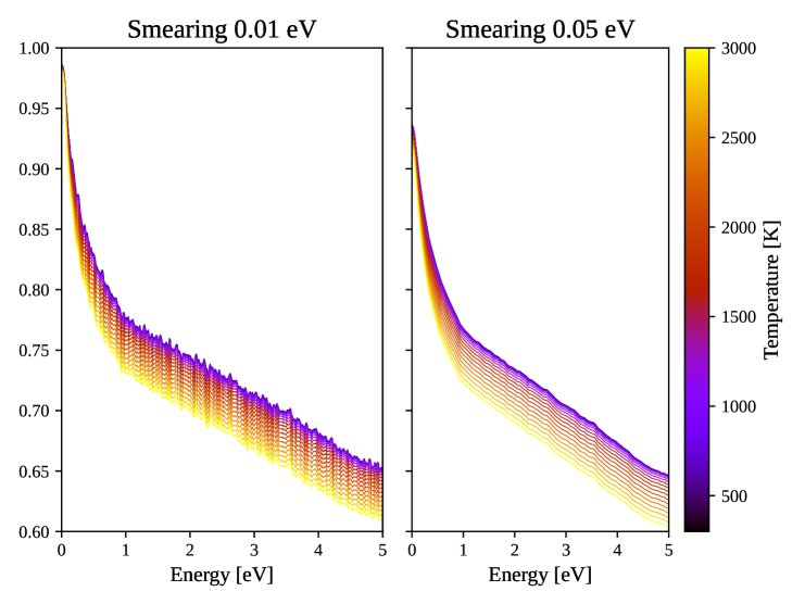
Figure 21: Convergence of the reflectivity as a function of the electronic temperature and smearing in the Cs-IV phase at approximately $660\text{\,}\mathrm{GPa}$.

The most important dependence introduced by the finite smearing is the drop of reflectivity at low frequency. This is due to the strong but trivial dependence of the Drude peak. In Figure 22 we show this effect, by plotting the real part of the conductivity as a function of smearing.

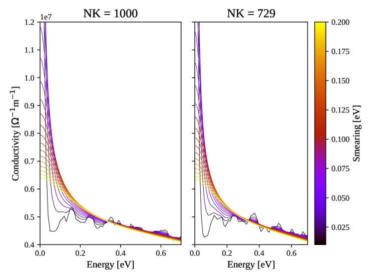
Figure 22: Convergence of the real conductivity as a function of smearing and number of k-points in the Cs-IV phase at approximately $660\text{\,}\mathrm{GPa}$.

Details on the DFT calculations

For the DFT calculations we employed the Quantum Espresso (?, ?) software suite, using a plane-wave basis set with a cutoff on the kinetic energy of $1088\text{\,}\mathrm{eV}$ ($4353\text{\,}\mathrm{eV}$ for the electronic density). We employed a norm-conserving pseudo-potential from the Pseudo Dojo library (?). To sample nuclear fluctuations within the SSCHA, the supercell contains 96 atoms for all the molecular structures (54 atoms for the atomic hydrogen with finite-size convergence checked against a 128 atoms supercell). The electronic $k$ mesh is reported for each structure in Table 2. In all cases, a Marzari-Vanderbilt smearing of $0.41\text{\,}\mathrm{eV}$ has been employed. Convergence of the energy with smearing and k-points is reported in Figure 23 and 24 for the Cmca-4 and Cs-IV structures, respectively. The Cmca-4 and Cs-IV phases are the ones with the most prominent metallic character, requiring the largest k-point sampling to converge.

	k-mesh
C2/c-24	$12\times 12\times 6$
P62/c-24	$12\times 12\times 6$
Cmca-12	$12\times 12\times 12$
Cs-IV	$48\times 48\times 48$
Cmca-4	$36\times 24\times 24$

Table 2: k-mesh employed for the DFT simulation of each phase. The Cmca-4 mesh is performed in the conventional unit cell containing 8 atoms.

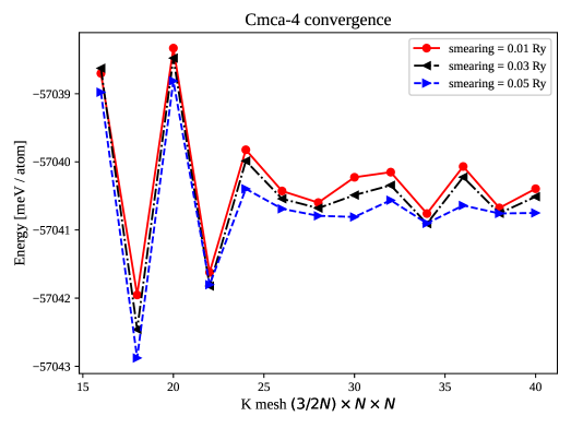
Figure 23: Molecular metallic Cmca-4 phase. DFT energy versus smearing and number of k-points in the primitive unit cell.

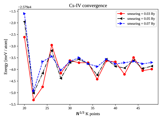
Figure 24: Atomic metallic Cs-IV phase. DFT energy versus smearing and number of k-points in the primitive unit cell.

Details on the DMC calculations

QMC calculations have been performed using the TurboRVB package (?). We carried out extensive DMC simulations in the lattice regularized DMC (LRDMC) flavor (?), to project the initial many-body wave function towards the ground state of the system within the fixed-node approximation (FNA) (?), and compute its energy.

As starting many-body state, we employed a Jastrow-Slater variational wave function $\Psi^{\textbf{k}}(\textbf{R})=\exp\{-U(\textbf{R})\}\det\{\phi^{\textbf{k}}_{j}(\textbf{r}^{\uparrow}_{i})\}\det\{\phi^{\textbf{k}}_{j}(\textbf{r}^{\downarrow}_{i})\}$ for $i,j\in\{1,\ldots,N/2\}$, where $N$ is the number of electrons in the unpolarized supercell, k is the twist belonging to a Monkhorst-Pack (MP) grid of the supercell Brillouin zone, and $\textbf{R}=\{\textbf{r}^{\uparrow}_{1},\ldots,\textbf{r}^{\uparrow}_{N/2},\textbf{r}^{\downarrow}_{1},\ldots,\textbf{r}^{\downarrow}_{N/2}\}$ is the $N$-electron coordinate.

$U$ is the Jastrow function, which is split into electron-nucleus, electron-electron, and electron-electron-nucleus parts: $U=U_{en}+U_{ee}+U_{een}$. The electron-nucleus function has an exponential decay and it reads as $U_{en}=\sum_{iI}J_{1b}(r_{iI})+U_{en}^{\textrm{no-cusp}}$, where the index $i$($I$) runs over electrons (nucleus), $r_{iI}$ is the electron-nucleus distance, and $J_{1b}(r)=\alpha(1-\exp\{-r/\alpha\})$, with $\alpha$ a variational parameter. $J_{1b}$ cures the nuclear cusp conditions, and allows the use of the bare Coulomb potential in our QMC framework. The electron-electron function has a Padé form and it reads as $U_{ee}=-\sum_{i\neq j}J_{2b}(r_{ij})$, where the indices $i$ and $j$ run over electrons, $r_{ij}$ is the electron-electron distance, and $J_{2b}(r)=0.5r/(1+\beta r)$, with $\beta$ a variational parameter. This two-body Jastrow term fulfills the cusp conditions for antiparallel electrons. The last term in the Jastrow factor is the electron-electron-nucleus function: $U_{een}=\sum_{(i\neq j)I}\sum_{\gamma\delta}M_{\gamma\delta I}\chi_{\gamma I}(r_{iI})\chi_{\delta I}(r_{jI})$, with $M_{\gamma\delta I}$ a matrix of variational parameters, and $\chi_{\gamma I}(r)$ a $(2s,2p,1d)$ Gaussian basis set, with orbital index $\gamma$, centered on the nucleus $I$. Analogously, the electron-nucleus cusp-free contribution to the Jastrow function, $U_{en}^{\textrm{no-cusp}}$, is developed on the same Gaussian basis set, such that $U_{en}^{\textrm{no-cusp}}=\sum_{iI}\sum_{\gamma}V_{\gamma I}\chi_{\gamma I}(r_{iI})$, where $V_{\gamma I}$ is a vector of parameters. The $J_{1b}$ and $J_{2b}$ Jastrow functions have been periodized using a $\textbf{r}\rightarrow\textbf{r}^{\prime}$ mapping that makes the distances diverge at the border of the unit cell, as explained in Ref  (?). For the inhomogeneous $U_{een}$ part, the Gaussian basis set $\chi$ has been made periodic by summing over replicas translated by lattice vectors.

The one-body orbitals $\phi$ are expanded on a primitive $(4s,2p,1d)$ Gaussian basis set, which we contracted into 6 hybrid orbitals, by using the geminal embedding orbitals (GEO) contraction scheme (?) at the $\Gamma$ point. $\phi$s’ are made periodic by using the same scheme as for the $\chi$s’. We verified that this basis set yields a FN-LRDMC bias in the energy differences smaller than the target error of 1 meV per atom. For each k belonging to the MP grid of a given supercell, we performed independent DFT calculations in the local density approximation (LDA) to generate $\{\phi^{\textbf{k}}_{j}\}_{j=1,\ldots,N/2}$ for all occupied states. Note that these LDA calculations are done for an ab initio Hamiltonian with bare Coulomb potential for the electron-ion interactions. This is thanks to the one-body Jastrow factor included in the DFT wave function, with $\alpha\approx 2.5$. In presence of a Coulomb divergence, fulfilling the ion cusp conditions accelerates enormously the basis set convergence already at the DFT level.

Before running LRDMC calculations, we optimized the $\alpha$, $\beta$ and $M_{\gamma\delta I}$ parameters, by minimizing the variational energy of the wave function $\Psi$ within the QMC linear optimization method (?), by keeping the orbitals $\phi^{\textbf{k}}_{i}$ fixed. All k twists belonging to the same system share the same set of optimal variational parameters for the Jastrow factor. The LRDMC projection is carried out at the lattice space $a=0.25a_{0}$, which yields converged energy differences. The projection algorithm has been implemented with a fixed population of 256 walkers per twist for the largest system sizes. The population bias, falling within the error bars, has been corrected by the “correcting factors” scheme (?).

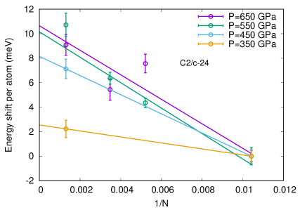
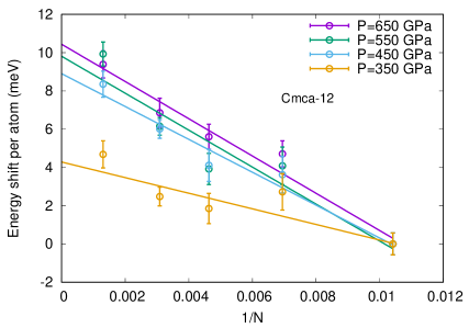
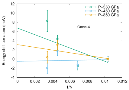
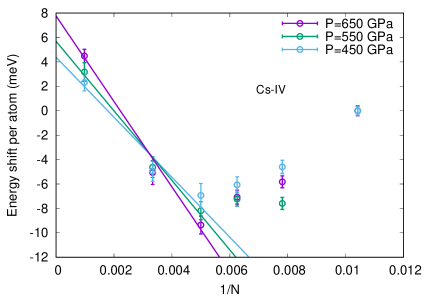
Figure 25: QMC finite-size scaling and extrapolation to the thermodynamic limit. KZK-corrected LRDMC energies for 4 crystalline symmetries (C2/c-24, Cmca-12, Cmca-4, and Cs-IV) plotted as a function of $1/N$, where $N$ is the number of atoms, with respect to their value at $N=96$, taken as reference. The energies are twisted-averaged in the canonical ensemble over a k-grid that has been rescaled according to the size of the supercell, as explained in the text. Note that despite the KZK correction and the canonical k-average, there is a residual size dependence beyond $N=96$, larger than the target accuracy of 1 meV per atom, that needs to be extrapolated. As expected, this residual dependence is stronger in the atomic metallic phase and in the molecular phases under high pressure, where the metallic character is enhanced.

For each lattice symmetry and volume $V$, we performed a size-scaling analysis to extrapolate the energies to the thermodynamic limit (see Fig. 25). Let $N_{x}\times N_{y}\times N_{z}$ be the electronic k-mesh yielding converged DFT results. In QMC, we used the same k-meshes reported in Tab. 2, except for the Cs-IV and Cmca-4 symmetries, where we used a slightly smaller $24\times 24\times 24$ and $18\times 12\times 12$ mesh, respectively. To further reduce finite-size errors, the k-mesh of the metallic Cs-IV symmetry has been centered at $(\pi,\pi,\pi)$, while the other k-grids are centred at $\Gamma$. We then took supercells with volume $V_{s}=L_{x}L_{y}L_{z}V$, where $L_{i}$ are the number of unit-cell replica in the $i$-th direction. Accordingly, the twists have been taken as belonging to the $M_{x}\times M_{y}\times M_{z}$ MP $\mathbf{k}$ mesh with $M_{i}=\textrm{int}[N_{i}/L_{i}]$, where int is the integer function. The ground state energies have been extrapolated by using supercells as large as $N=768$ for the molecular phases, while for atomic I4/amd-2 symmetry we used supercells as large as $N=1024$. The final extrapolations have been performed by a linear fitting in $1/N$, computed with Kwee-Zhang-Krakauer (KZK)-corrected energies (?).

We also investigated the role of the FNA in DMC, by exploiting the capabilities of TurboRVB for optimizing the Slater orbitals $\phi^{\textbf{k}}_{i}$. Due to the increased cost of these simulations, we performed the nodal optimization by the variational Monte Carlo energy minimization at the special k-point only (?). The corresponding DMC energies computed by projecting wave functions with relaxed nodes prove that the FN bias does not affect the relative energies between molecular phases. However, the optimization of the FNA with respect to the LDA nodes in the QMC wave function shifts the atomic-phase energy upwards by about $3\text{\,}\mathrm{meV}$ per atom (see Tab. 3), also shifting the transition pressure by $20\text{\,}\mathrm{GPa}$ towards higher pressures (the correct value is accounted for in the phase diagram of Figure 2).

symmetry	1.416 Å3	1.259 Å3	1.115 Å3
C2/c-24	6.2 ($\pm$ 1.7)	-	-
P62/c-24	6.0 ($\pm$ 1.7)	-	-
Cmca-4	5.9 ($\pm$ 1.5)	-	-
Cmca-12	7.2 ($\pm$ 1.1)	6.5 ($\pm$ 1.1)	6.1 ($\pm$ 1.0)
Cs-IV	-	3.4 ($\pm$ 0.8)	3.2 ($\pm$ 0.8)

Table 3: Fixed node LRDMC energy gain (in meV/H) at different volumes with respect to the LDA nodes after full wave function optimization at the special k point. The energy optimization has been performed at the variational Monte Carlo level for supercells up to $N=288$. It turns out that the LRDMC energy gain due to the nodal optimization has a very weak system size dependence. $N=96$ gives already converged results for the FN energy gain.

We ran all LRDMC calculations long enough to reach a stochastic error bar around the target accuracy of $1\text{\,}\mathrm{meV}$ per atom.

DMC correction of the DFT exchange-correlation energy

To correct for the DFT exchange-correlation error, we computed DMC energies at each centroids structure. For each structure, we fitted the energy difference between DFT and DMC for the same structure as a function of the density, and added it on the top of the DFT energy-volume relationship, computed on a much denser volume grid thanks to the cheaper cost of DFT. With this procedure, we do not rely on any phenomenological definition of the equation of states (EOS), such as the Birch-Murnaghan or Vinet EOS, in order to get QMC-interpolated energy-versus-volume curves. Fitting the DMC corrections with respect to an underlying ab initio theory is easier than fitting directly the DMC total energies. Indeed, total energies show a much larger dependence on the volume than energy corrections. The plot of the QMC corrections is reported in Figure 26. In this plot, the QMC corrections are obtained from DMC energies computed within the fixed-node approximation (FNA) and with DFT-LDA nodes.

Figure 26: QMC energy corrections. Electronic energy differences between DFT-BLYP and DMC calculations at hydrogen centroid positions obtained from SSCHA nuclear quantum fluctuations evaluated at the DFT-BLYP level. The DMC energies are computed within the FNA with DFT-LDA nodes. The fit is a straight line for all phases.

Fig. 26 shows that the difference between phases smears out when the density increases, pointing toward a better DFT description above densities corresponding to $800\text{\,}\mathrm{GPa}$, where the electronic behavior of the system is more similar to the jellium model. This regime, however, kicks in at pressures above the range of interest for this work. It is worth noting that the smallest absolute values of the DMC correction with respect to DFT-BLYP are found for the atomic and Cmca-4 phases. This is the reason why accounting for DMC corrections is fundamental to correctly reproduce the hydrogen atomization: all molecular phases, except for Cmca-4, are lowered in energy with a consequent shift of the atomization transition toward higher pressures.

We have mentioned that the QMC corrections reported in Figure 26 are based on DMC calculations within the FNA and with DFT-LDA nodes. As explained in the QMC calculations details, we assessed the quality of the DFT-LDA wave-function nodes that are kept fixed during the DMC projection in the FNA. This is the only bias present in the DMC energies, which would otherwise have been exact. We have been able to relax the nodes at the variational Monte Carlo level, and then use improved nodes in DMC. According to Tab. 3, a systematic gain of 3meV/H is found after nodal optimization in DMC energies for the molecular phases with respect to the atomic one. It appears that the gain is the same for all molecular structures (within the error bars) and it is volume independent in the range of pressures explored in this work. This 3meV/H shift is added to the QMC corrections in Fig. 26 to yield the final corrections, used to compute the QMC phase diagram of Figure 2. It adds up to further disfavor the atomic phase, whose stability is pushed up to higher pressures in the phase diagram.

DMC+SSCHA systematic errors

Our approach of combining DMC energy corrections and SSCHA anharmonic vibrational contributions in an additive way relies upon the hypothesis that DMC corrections depend mainly on the phase and pressure (or volume), and very weakly on the particular atomic displacement around the centroids within a given phase. To test this hypothesis and give an estimate of the systematic error introduced by this approximation, we repeated the same calculations by choosing a different reference structure to compute the DMC shifts. Therefore, we replaced the SSCHA centroids of hydrogen with those of deuterium to change reference structure, and we went again through all steps by using this time the DMC correction computed on the D centroids, for validation and error quantification.

In Figure 27, we compare the DMC corrections computed for the SSCHA centroids of H and D, respectively, employing supercells of 96 nuclei in the DMC calculations. In this way, we can check whether the DMC shifts are independent of specific ionic distortion, by retaining a dependence only on the overall arrangement, i.e. on the crystalline symmetry. The plots in panels a) and b) show that the shift between C2/c-24 and Cmca-12 depends only slightly on the centroid position, while the atomic phase is more sensitive to the choice of the centroid. This discrepancy is mainly due to the difference in the c/a equilibrium values of Cs-IV between DMC and DFT-BLYP (see Section on the Cs-IV phase).

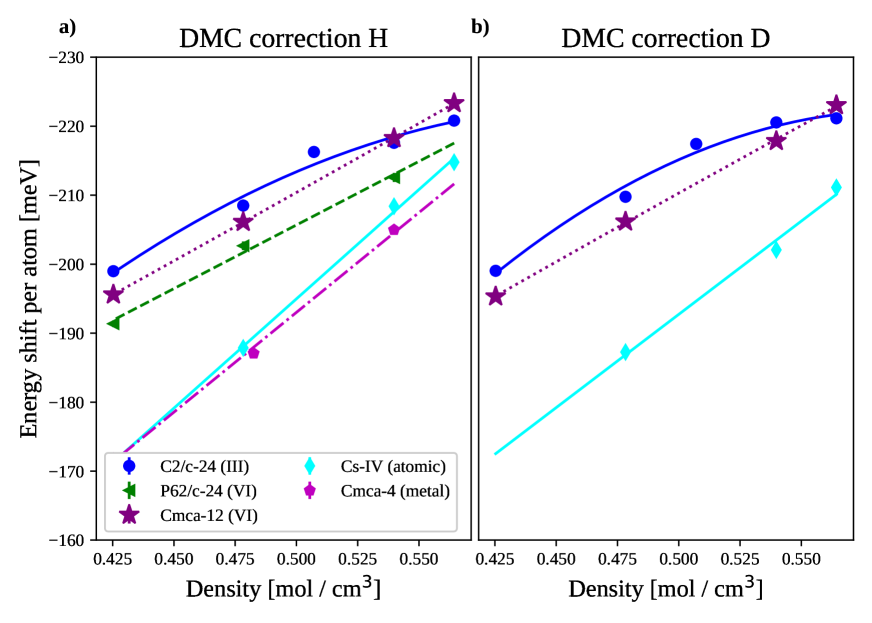
Figure 27: Electronic energy difference per atom between DMC and DFT calculations on the same BLYP structures. Here, we used the KZK-corrected LRDMC energies computed at $N=96$ for all phases reported in the plot, before full thermodynamic extrapolation. This allows for a direct comparison with deuterium, where we did not perform an explicit finite-size extrapolation as we did in hydrogen (see Fig. 25). Panel a: the energy shift per atom is computed on the SCHA centroid positions with mass equal to hydrogen. Panel b: the energy shift is computed on structures with SCHA centroid positions for deuterium.

In Figure 28, we show the phase diagram obtained by considering the DMC correction on the D centroids. Here, the DMC energies computed on the D centroids are extrapolated to the thermodynamic limit by assuming the same $1/N$ dependence as found in protium. Therefore, the most accurate DMC correction of the BLYP exchange-correlation energy is obtained for the H-centroids geometries, where an explicit and computational time-consuming extrapolation to the thermodynamic limit has been performed explicitly. Nonetheless, the phase diagram in Figure 28 is valuable for estimating the systematic errors. This can be done by direct comparison with the phase diagram drawn in Figure 10, obtained instead by relying upon the H-centroids DMC correction.

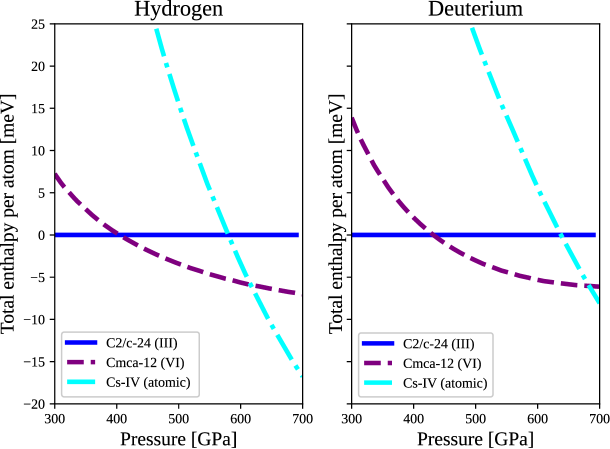
Figure 28: Full phase diagram, considering DMC corrections and nuclear quantum effects. DMC corrections are evaluated using the SSCHA centroids of deuterium.

Based on the phase diagrams plotted in Figs. 10 and 28, we report the phase-transition pressures for hydrogen and deuterium in Tabs. 4 and 5, respectively. The discrepancies between the results is used as an estimate of the systematic error in the final phase diagram, shown in Figure 2.

	III $\rightarrow$ VI	VI $\rightarrow$ ATOMIC
H-centroids DMC correction	$422\text{\,}\mathrm{GPa}$	$575\text{\,}\mathrm{GPa}$
D-centroids DMC correction	$404\text{\,}\mathrm{GPa}$	$616\text{\,}\mathrm{GPa}$

Table 4: The final phase-transition pressures for H obtained with DMC energy correction estimated based on H or D centroids. The results obtained from the H-centroids based DMC correction are taken as the most accurate in the main text. The ones obtained from the D-centroids based DMC correction provide an estimation of systematic error introduced by the approximation.

	III $\rightarrow$ VI	VI $\rightarrow$ ATOMIC
H-centroids DMC correction	$452\text{\,}\mathrm{GPa}$	$646\text{\,}\mathrm{GPa}$
D-centroids DMC correction	$432\text{\,}\mathrm{GPa}$	$683\text{\,}\mathrm{GPa}$

Table 5: Same transition pressures as in Fig. 4, but for deuterium. The results obtained from the H-centroids based DMC correction are taken as the most accurate in the main text. The ones obtained from the D-centroids based DMC correction provide an estimation of systematic error introduced by the approximation.

References

- 1. N. W. Ashcroft, Phys. Rev. Lett. 21, 1748 (1968).
- 2. H.-k. Mao, R. J. Hemley, Reviews of modern physics 66, 671 (1994).
- 3. R. T. Howie, C. L. Guillaume, T. Scheler, A. F. Goncharov, E. Gregoryanz, Physical Review Letters 108 (2012).
- 4. P. Dalladay-Simpson, R. T. Howie, E. Gregoryanz, Nature 529, 63 (2016).
- 5. P. Loubeyre, F. Occelli, P. Dumas, Nature 577, 631 (2020).
- 6. M. I. Eremets, A. P. Drozdov, P. P. Kong, H. Wang, Nature Physics (2019).
- 7. R. P. Dias, I. F. Silvera, Science 355, 715 (2017).
- 8. M. Borinaga, J. I. nez Azpiroz, A. Bergara, I. Errea, Physical Review Letters 120, 057402 (2018).
- 9. A. F. Goncharov, V. V. Struzhkin, Science 357 (2017).
- 10. I. F. Silvera, R. Dias, Science 357, eaan2671 (2017).
- 11. P. Loubeyre, F. Occelli, P. Dumas, ArXiv e-prints (2017).
- 12. C. Ji, et al., Nature 573, 558 (2019).
- 13. D. M. Straus, N. W. Ashcroft, Physical Review Letters 38, 415 (1977).
- 14. I. Errea, et al., Physical Review Letters 114 (2015).
- 15. I. Errea, et al., Nature 578, 66 (2020).
- 16. N. D. Drummond, et al., Nature Communications 6 (2015).
- 17. W. M. C. Foulkes, L. Mitas, R. J. Needs, G. Rajagopal, Reviews of Modern Physics 73, 33 (2001).
- 18. I. Errea, M. Calandra, F. Mauri, Physical Review B 89 (2014).
- 19. R. Bianco, I. Errea, L. Paulatto, M. Calandra, F. Mauri, Physical Review B 96 (2017).
- 20. L. Monacelli, I. Errea, M. Calandra, F. Mauri, Phys. Rev. B 98, 024106 (2018).
- 21. L. Monacelli, et al., Journal of Physics: Condensed Matter 33, 363001 (2021).
- 22. J. McMinis, R. C. Clay, D. Lee, M. A. Morales, Physical Review Letters 114 (2015).
- 23. S. Azadi, N. D. Drummond, W. M. C. Foulkes, Physical Review B 95 (2017).
- 24. B. Monserrat, et al., Physical Review Letters 120 (2018).
- 25. S. Azadi, B. Monserrat, W. Foulkes, R. Needs, Physical Review Letters 112 (2014).
- 26. B. Miehlich, A. Savin, H. Stoll, H. Preuss, Chemical Physics Letters 157, 200 (1989).
- 27. C. J. Pickard, R. J. Needs, Nature Physics 3, 473 (2007).
- 28. L. Monacelli, I. Errea, M. Calandra, F. Mauri, Nature Physics (2020).
- 29. M. Borinaga, I. Errea, M. Calandra, F. Mauri, A. Bergara, Phys. Rev. B 93, 174308 (2016).
- 30. T. Morresi, L. Paulatto, R. Vuilleumier, M. Casula, The Journal of Chemical Physics 154, 224108 (2021).
- 31. F. Tran, P. Blaha, Physical Review Letters 102 (2009).
- 32. V. Gorelov, M. Holzmann, D. M. Ceperley, C. Pierleoni, Phys. Rev. Lett. 124, 116401 (2020).
- 33. M. Nimier-David, D. Vicini, T. Zeltner, W. Jakob, ACM Transactions on Graphics 38, 1 (2019).
- 34. C. Zhang, et al., Physical Review B 98 (2018).
- 35. G. Prandini, G.-M. Rignanese, N. Marzari, npj Computational Materials 5 (2019).
- 36. R. C. Clay, et al., Physical Review B 89 (2014).
- 37. H. T. Stokes, D. M. Hatch, Journal of Applied Crystallography 38, 237 (2005).
- 38. A. Togo, I. Tanaka, arXiv preprint arXiv:1808.01590 (2018).
- 39. P. Borlido, et al., Journal of Chemical Theory and Computation 15, 5069 (2019).
- 40. P. Giannozzi, et al., Journal of Physics: Condensed Matter 21, 395502 (2009).
- 41. P. Giannozzi, et al., Journal of Physics: Condensed Matter 29, 465901 (2017).
- 42. D. R. Hamann, Phys. Rev. B 88, 085117 (2013).
- 43. K. Nakano, et al., The Journal of Chemical Physics 152, 204121 (2020).
- 44. M. Casula, C. Filippi, S. Sorella, Physical review letters 95, 100201 (2005).
- 45. J. B. Anderson, The Journal of Chemical Physics 65, 4121 (1976).
- 46. S. Sorella, N. Devaux, M. Dagrada, G. Mazzola, M. Casula, The Journal of chemical physics 143, 244112 (2015).
- 47. C. Umrigar, J. Toulouse, C. Filippi, S. Sorella, R. G. Hennig, Physical review letters 98, 110201 (2007).
- 48. M. C. Buonaura, S. Sorella, Physical Review B 57, 11446 (1998).
- 49. H. Kwee, S. Zhang, H. Krakauer, Physical review letters 100, 126404 (2008).
- 50. M. Dagrada, S. Karakuzu, V. L. Vildosola, M. Casula, S. Sorella, Physical Review B 94, 245108 (2016).
Acknowledgments
L.M. acknowledges CINECA under the ISCRA initiative for providing high performance computational resources employed in this work. M.C. thanks GENCI for providing computational resources under the grant number 0906493, the Grands Challenge DARI for allowing calculations on the Joliot-Curie Rome HPC cluster under the project number gch0420. M.C., K.N., and S.S. thank RIKEN for providing computational resources of the supercomputer Fugaku through the HPCI System Research Project (Project ID: hp210038). K.N. acknowledges support from the JSPS Overseas Research Fellowships, from Grant-in-Aid for Early Career Scientists (Grant No. JP21K17752), and from Grant-in-Aid for Scientific Research (Grant No. JP21K03400). S.S. acknowledges support from MIUR, PRIN-2017BZPKSZ. This work was supported by the European Centre of Excellence in Exascale Computing TREX-Targeting Real Chemical Accuracy at the Exascale. This project has received funding from the European Union’s Horizon 2020 Research and Innovation program under Grant Agreement No. 952165.