Patch-NetVLAD+: Learned patch descriptor and weighted matching strategy
for place recognition

Abstract

Visual Place Recognition (VPR) in areas with similar scenes such as urban or indoor scenarios is a major challenge. Existing VPR methods using global descriptors have difficulty capturing local specific regions (LSR) in the scene and are therefore prone to localization confusion in such scenarios. As a result, finding the LSR that are critical for location recognition becomes key. To address this challenge, we introduced Patch-NetVLAD+, which was inspired by patch-based VPR researches. Our method proposed a fine-tuning strategy with triplet loss to make NetVLAD suitable for extracting patch-level descriptors. Moreover, unlike existing methods that treat all patches in an image equally, our method extracts patches of LSR, which present less frequently throughout the dataset, and makes them play an important role in VPR by assigning proper weights to them. Experiments on Pittsburgh30k and Tokyo247 datasets show that our approach achieved up to 6.35% performance improvement than existing patch-based methods.

1 Introduction

Visual Place Recognition (VPR) is the task to estimate the location of a query image by recognizing the same place in a set of database images. VPR has achieved significant progress with the advances of convolutional neural networks (CNN) [1, 6, 8, 21]. However, VPR is still a challenging task in areas with similar scenes such as urban or indoor scenes. There are two common ways to address this challenge: improving the performance of descriptor or improving the match strategy.

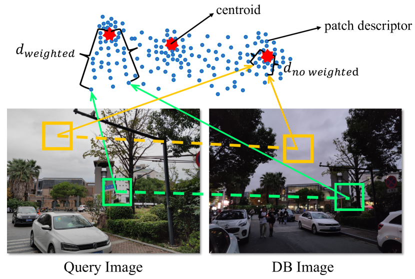
Figure 1: Comparing weighted and unweighted matching. The yellow patches located in the sky are frequently present in scenes. Therefore, they are depicted close to a centroid (red) of the description space. Therefore they should play an insignificant role in the VPR. On the contrary, patches in LSR (e.g. green patches covering the signage) appear only in a few scenes. Their descriptors are far from the centroids. We propose to assign weights to patches based on the distance between patch descriptors and centroids in the description space so that patches in LSR play an important role in image matching.

Most of the methods to improve descriptor performance design a novel CNN for extracting global descriptors. These global descriptors[1, 6, 7] which describe the whole image typically excel in terms of their robustness to appearance and illumination changes, as they are directly optimized for place recognition. However, as shown in [23, 10, 29], in areas with similar scenes, the global descriptor has difficulty distinguishing differences between local regions.

Our method takes the same strategy as Patch-NetVLAD[10], which uses a sliding window to generate patches and then derives patch descriptors from NetVLAD to achieve place recognition. However, Patch-NetVLAD extracted patch descriptors using NetVLAD trained on the whole image, which is not accurate. Inspired by SFRS[8], our method uses triplet loss fine-tune NetVLAD to make it more suitable for extracting patch-level descriptors. However, GNSS-based labels of public datasets only provide image-to-image similarities. To tackle this problem, patch-to-patch similarities and matches of local keypoint are used to select the positive and negative patch training set required by the triplet loss function.

The methods to optimize the matching strategy are mainly based on intra-set similarities[19, 22] and sequence searching [5, 17]. Unlike patch-based methods, these methods optimized the VPR by matching multiple query images, rather than improving the matching performance of a single image. Besides, these methods required multiple query images. The patch-based VPR method decomposed the image into patches, and therefore, utilized the local regions for matching. Rather than treating all the patches equally, we found that the importance of different patches in pairwise image matching varies. Therefore, it is critical to find patches in local specific regions (LSR) that are crucial for place recognition.

We propose to cluster the patch descriptors of the whole dataset in the description space, and patches far away from centroids are considered as patches in LSR as they occur less frequently in the dataset. As shown in Figure 1, patches located in the frequently present sky are closer to a centroid while patches covering the signage which appear infrequently are far from the centroids. Inspired by this, by assigning a greater weight to patches in LSR than other patches, we make them play an important role in image matching.

In summary, our contributions are summarised as follows:

1. We propose a novel method to fine-tune NetVLAD using triplet loss to make it more suitable for extracting patch-level descriptors. The positive and negative patches of triplet loss function are selected by patch-to-patch similarities and matches of local keypoint.

2. We propose to assign weights to patches in LSR based on distances of patch descriptors from the centroids in the description space throughout the dataset. The weighted patches are then used to optimize the pairwise image matching.

2 Related Work

Existing works on VPR enhancement can be grouped into descriptor-centered and strategy-centered, where the former improved the accuracy and robustness of VPR by designing a novel descriptor, while the works based on the strategy utilized inter-image relationships to optimize VPR.

2.1 Descriptor-centered Methods

Global Image Descriptor: Early global descriptor approaches focused on statistical information of the image, such as color histograms[27] and linear image features[14]. Global image descriptor can be aggregated from the local keypoint descriptor, e.g. WI-SURF[2], ERIEF-Gist[24], Bag of Words (BoW)[12], Vector of Locally Aggregated Descriptors (VLAD)[11] and Fisher Vectors (FV)[20], etc. Inspired by VLAD, [1] designed an end-to-end (CNN) architecture NetVLAD that aggregates local descriptors according to learnable centroids. Benefiting from the success of NetVLAD, Contextual Reweighting Network (CRN)[13], added a spatial attention mechanism before the VLAD layer to focus on regions that positively contribute to VPR. For the same purpose as CRN, Attention-based Pyramid Aggregation Network (APANet)[30] encode the multi-size buildings by using spatial pyramid pooling, and suppress the confusing region while highlight the discriminative region by attention block. However, both CRN and APANet require re-training on the whole dataset.

In order to deal with the problem caused by the opposite viewpoint, [6] proposed a novel image descriptor by combining semantic labels and appearance. However, [6] just encodes semantic regions in images by [15] and simply concatenates them as global descriptors. In addition, only three types of semantic regions were considered, therefore, it is not valid for images that do not contain these regions.

Patch/Region Descriptor: This kind of methods computes image descriptors only using relevant patches of an image rather than the whole image. These methods focus on the regions of interest (e.g., landmarks) of an image. Most of these methods adopt existing object proposal techniques to extract regions or patches. [23] proposed a landmark-based VPR method by combining the CNN features of landmarks detected by Edge Box[31]. Unlike [23], [4] only used CNN once to detect landmarks and extract their features. [6] retrained RefineNet[15] to get semantic regions (e.g., road, building and vegetation) and their descriptors (LoST).

[28] proposed a new landmark generation method named MSW (multi-scale sliding window). MSW performed better than object proposal techniques due to the use of the sliding window, especially when illumination or viewpoint changes. Similar to MSW, Patch-NetVLAD[10] also used the sliding window to generate multi-scale patches and obtained patch descriptors from NetVLAD residuals. However, these patches are described using NetVLAD trained on the whole image, which is not accurate.

In a general sense, for similar scenes, though the images are similar as a whole, there may still be some dissimilar regions in the images. Therefore, we also use a sliding window to acquire patches but fine-tune NetVLAD to make it more suitable for patch descriptor extraction.

2.2 Strategy-centered Methods

SeqSLAM[17] changed the VPR problem from calculating the single location globally to finding a local best candidate within each local sequence. Similar ideas were proposed in[9, 18]. However, most of these sequence-based methods are designed to improve the performance of VPR rather than to guide the single image to match correctly. [19] optimized image matching by considering the relationships within the query dataset; in detail, it inhibits multiple query descriptors that are mutually different from matching to the same database descriptor, but the method is no longer valid when there is only one query image. [29] proposed a regional relation module to model the relation information between regions of an image, although this method considers the importance of different regions in the image, the extraction and importance of regions are included in the network training, which is closely related to the training set with poor generalization performance, while our method is explicit and has little related to the training set.

Patch-NetVLAD[10] first found the candidate images using NetVLAD, and then calculated the patch match score for each pair of images to rank the candidate images and determine the best matching image. However, Patch-NetVLAD treated all patches equally when matching patches.

Different from Patch-NetVLAD, our method tried to find patches in LSR and differentiated patches according to their contributions to VPR.

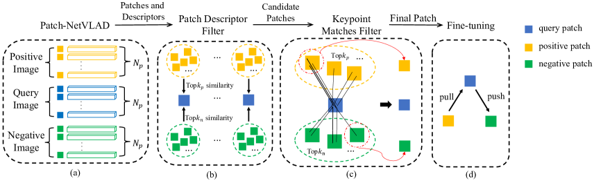
Figure 2: The pipeline of fine-tuning the NetVLAD for patches. (a) The patches are extracted in the images using a sliding window; (b) For each query patch we find $Top\ k_{p}$ similar patches in the positive image using the patch descriptors extracted from the original NetVLAD, and use these patches as the candidate positive patches; the candidate negative patches are the $Top\ k_{n}$ similar patches found from the negative image. (c) After that, the final positive patch and negative patches are chosen from candidate patches based on the result of keypoint matching. For clarity, a query image only selects one positive image and one negative image in the figure. (d) The triplet loss-based fine-tuning results in pulling the descriptors of positive patches and query patch together while pushing the descriptors of negative patches and query patch apart.

3 Methodology

In this section, we will introduce our method in detail. Our approach consists of two parts, the first part describes the extraction of patch-level descriptors; the second part describes how to find and assign weights to patches based on their descriptors, and how to make these weighted patches optimize the matching of image pairs.

The notations we will use throughout the paper are as follows: we denote $P_{i}^{source}$ as a patch $i$, and its descriptor $f_{i}^{source}$, where $source$ can be $db$ the entire database set, $q$ the query image, $p$ the positive image, $n$ the negative image, and $r$ the reference image. $N_{p}^{source}$ represents the number of patches in the $source$.

3.1 Patch-level Descriptor

3.1.1 Patch and patch descriptor

Similar to [10], we use a sliding window to extract square patches from the feature map (conv5 layer for VGG16) $F\in\mathbb{R}^{H\times W\times D}$. For each image, we can obtain a total of $N_{p}$ patches$\{P_{i}\in\mathbb{R}^{(d_{p}\times d_{p})\times D}\}_{i=1}^{N_{p}}$, and

$$N_{p}=\left\lfloor\frac{H-d_{p}}{s_{p}}+1\right\rfloor\times\left\lfloor\frac{W-d_{p}}{s_{p}}+1\right\rfloor,d_{p}\leqslant min(H,W)$$ (1)

where $d_{p}$ is the side length of the square patch, $s_{p}$ is the stride of the sliding window.

For each patch, we extract its descriptor $\{f_{i}\in\mathbb{R}^{1\times D_{pca}}\}_{i=1}^{N_{p}}$ by using a VLAD aggregation layer followed by a projection layer and principle component analysis (PCA). Concretely, the VLAD aggregation layer $l_{VLAD}$ aggregates the $(d_{p}\times d_{p})\times D$-dimensional features into a $K\times D$-dimensional matrix by applying a weighted sum soft-assignment to the residuals between each feature and K learned centroids. Then, the projection layer $l_{proj}$ reshapes the resultant matrix into a vector by applying intra-normalization in its column followed by L2-normalization in its whole. And finally, PCA $l_{pca}$ with whitening is applied to reduce the dimension of the output descriptor. More details can be found in [1] [10].

3.1.2 The selection of positive and negative patches

Accurate extraction of positive and negative patches is the key to patch descriptor fine-tuning, and the pipeline is shown in Figure 2 (a)-(c).

We first use the weak GPS labels provided by the dataset to find the positive image and the negative image. Subsequently, patches $\{P_{i}^{q}\}_{i=1}^{N_{p}}$ ($\{P_{i}^{p}\}_{i=1}^{N_{p}}$,$\{P_{i}^{n}\}_{i=1}^{N_{p}}$) and their descriptors$\{f_{i}^{q}\}_{i=1}^{N_{p}}$ ($\{f_{i}^{p}\}_{i=1}^{N_{p}}$,$\{f_{i}^{n}\}_{i=1}^{N_{p}}$) are extracted from the query image, positive image, negative image respectively as labels for training (Figure 2 (a)).

As shown in Figure 2 (b), each patch located in the query image is regarded as a candidate query patch $\{P_{i}^{q}\}_{i=1}^{N_{p}}$. For each candidate query patch, the most $k_{p}$ similar patches from the positive image are selected as the candidate positive patches $\{P_{i}^{p}\}_{i=1}^{k_{p}}$ using the Cosine distance of their descriptors. Similarly, the most $k_{n}$ similar patches from the negative image are selected as the candidate negative patches $\{P_{i}^{n}\}_{i=1}^{k_{n}}$.

However, the selected candidate patches are not accurate yet because the descriptors were derived from the original NetVLAD. Therefore, we extract dense keypoints [16] in the images and match between the query image and its corresponding positive and negative candidate images, followed by GCRANSAC[3] filtering. Then, we keep the patches with matching keypoints as the final query patches $\{P_{i}^{q\_f}\}$. The one with the most matching keypoints from the candidate positive patches is selected as the final positive patch $\{P_{i}^{p\_f}\}$, and the one with the least number of matched keypoints from the candidate negative patches is selected as the final negative patches $\{P_{i}^{n\_f}\}$.This is demonstrated in Figure 2 (c).

3.1.3 Fine-tune the NetVLAD

The query patch $\{P_{i}^{q\_f}\}$ and the corresponding positive patch $\{P_{i}^{p\_f}\}$ and negative patches $\{P_{i}^{n\_f}\}$ are used to fine-tune the original NetVLAD with a triplet loss. Triplet loss for patches is defined as:

$$loss=\sum_{j}l\bigg{(}\min_{i}\big{(}d_{cos}(P^{q},P_{i}^{p})\big{)}+m-d_{cos}(P^{q},P_{j}^{n})\bigg{)}$$ (2)

where $l$ is the hinge loss $l(x)=\max(x,0)$, and $m$ is a constant parameter giving the margin.

The triplet loss pulls the positive patches and query patch together, i.e. reducing their Cosine distance, while pushes the negative patches and query patch apart, i.e. increase their Cosine distances (Figure 2 (d)).

3.2 Weighted patch-based matching

3.2.1 Patch weightings

We aim to find patches in LSR and assign weights to patches according to their contributions in VPR. A fact is that patches with few occurrences in the DB can be considered as special patches, and a large weight can be assigned to these patches to make them play a major role in VPR. However, even with a fine-tuned descriptor, it is not able to assess the occurrence of a patch. Therefore, our approach measures patch specificity by computing the distance between the patch and the dataset, and more specifically, the distance between the patch and the centroids of the DB dataset.

We first extract a patch descriptors set $\{f_{i}^{db}\in\mathbb{R}^{1\times D_{pca}}\}_{i=1}^{N_{p}^{db}}$ from the images of the entire DB dataset. Then, K-means is employed to cluster these patch descriptors to obtain K centroids $\{f_{i}^{c}\in\mathbb{R}^{1\times D_{pca}}\}_{i=1}^{k}$, and these centroids represent the distribution of similar patch descriptors in the description space.

The distances between a patch descriptor and centroids can be computed using the Cosine distance. The patches that far away from most of the centroids are considered as special patch, so we define the weighting as following:

$$w(f)=\sum_{i}^{\alpha}\{d_{cos}(f,f_{i}^{c})\}_{\min_{\alpha}}$$ (3)

where $f$ is the descriptor of the patch that needs to be weighted, $\{\}_{\min_{\alpha}}$ represent a subset of $\alpha$ smallest items.

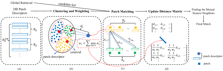
Figure 3: The weighted matching strategy. (a)(b) Using K-means to cluster the patch descriptors of the whole DB dataset, patches are weighted according to the distances between the patch descriptors and centroids. (c) The distance matrix is derived by exhaustively matching the patches of image pairs. (d) The distance matrix is updated by multiplying the weights of the corresponding patches, the mutual nearest neighbors Equation 4 is optimized based on the updated distance matrix.

3.2.2 Image pair matching

[10] proposed a hierarchical strategy to find the best matching image of a query image. First, it used the original NetVLAD description to retrieve the top100 images that are most similar to the query image. Then, it computed the patch descriptors and perform patch-level matching by finding the mutual nearest neighbors $\mathcal{P}$ by Equation 4:

$$\mathcal{P}=\{(i,j):i=NN_{r}(f_{j}^{q}),j=NN_{q}(f_{i}^{r})\}$$ (4)

where $NN_{r}(f)=argmin_{i}\big{(}d_{cos}(f,f_{i}^{r})\big{)}$ and $NN_{q}(f)=argmin_{j}\big{(}d_{cos}(f,f_{j}^{q})\big{)}$ retrieve the nearest neighbors descriptor match with respect to Cosine distance within the query and reference image. According to the matched patches, the spatial matching score was computed to rank the top100 images, and the final image retrieval results are obtained.

Similarly, our method also ranks the initial retrieval image set by a similarity score between a pair of images.

Let the image pair list $L$ be:

$$L={(I_{q},I_{r})}$$ (5)

where $I_{q}$ is the query image, $I_{r}$ is a candidate image obtained by original NetVLAD. For each image pair in $L$, the patch descriptors are extracted and their distances are calculated to generate the distance matrix $\mathcal{D}$:

$$\mathcal{D}=\begin{bmatrix}d_{cos}(f_{1}^{q},f_{1}^{r})&d_{cos}(f_{1}^{q},f_{2}^{r})&\cdots\\ d_{cos}(f_{2}^{q},f_{1}^{r})&d_{cos}(f_{2}^{q},f_{2}^{r})&\cdots\\ \vdots&\vdots&\ddots\end{bmatrix}$$ (6)

In order to make the higher weighted patches located in the LSR play a bigger role in matching, we weighted the distance matrix to update $\mathcal{D}$. The weighted distance matrix is given by:

$$weighted\ \mathcal{D}=\\ \begin{bmatrix}\frac{1}{w(f_{1}^{q})}\frac{1}{w(f_{1}^{r})}&\frac{1}{w(f_{1}^{q})}\frac{1}{w(f_{2}^{r})}&\cdots\\ \frac{1}{w(f_{2}^{q})}\frac{1}{w(f_{1}^{r})}&\frac{1}{w(f_{1}^{q})}\frac{1}{w(f_{2}^{r})}&\cdots\\ \vdots&\vdots&\ddots\end{bmatrix}\circ\mathcal{D}$$ (7)

where $\circ$ means Hadamard product. By this means, patches with large weights can be matched easily, because their values in the distance matrix become smaller, while those with small weights are hardly matched.

4 Experiments

4.1 Experiment setup

We use two benchmark datasets to evaluate our method: Pittsburgh30k [26] and Tokyo247 [25]. Both datasets are captured at large-scale scenes that contain many similar scenes. Pittsburgh30k benchmark consists of three parts: train-set, val-set and test-set. The train-set contains 7416 queries and 10000 reference images; the val-set contains 7608 queries and 10000 reference images; the test-set contains 6818 queries and 10000 reference images. Tokyo247 consists of 315 queries and 75984 reference images. For a fair comparison, we follow the experiment settings of [10] and choose same queries as [10] of Pittsburgh30k and Tokyo247. In our experiment, we adopt the square patch with side length $d_{p}=5$ on feature map (the output of conv5 layer for VGG16) and Rapid Spatial Scoring proposed by [10].

During fine-tuning the NetVLAD, the training parameters are the same as [1]. We utilize the train-set of Pittsburgh30k for fine-tuning the original NetVLAD and the best model that achieves optimal performance on val-set is selected.

The original NetVLAD is used to extract the patch descriptors to find the candidate positive patches and negative patches. ASLFeat[16] is used to detect the keypoints on the image, after detecting keypoints, KNN match ($k=2$) is used to match keypoints followed by GCRANSAC[3] to remove the outlier match.

During weighted matching, we set the stride of the sliding window to $s_{p}=d_{p}=5$, i.e. there is no overlap between patches, the number of centroids is set to $k=16$ and $\alpha=10$ in Equation 3.

All datasets are evaluated using Recall@N metric, i.e. a query image is successfully retrieved from $topN$ if at least one of the $topN$ images is within 25 meters.

4.2 Comparison with the State-of-the-art

Table 1: Quantitative results

Method	Pittsburgh30k			Tokyo247
	R@1	R@5	R@10	R@1	R@5	R@10
NetVLAD[1]	83.66	91.77	94.04	66.89	78.10	80.95
Patch-NetVLAD[10]	87.40	93.66	95.36	77.14	84.44	86.98
Ours	88.50	94.47	95.79	83.49	87.94	90.16

$\begin{array}[]{cc}\includegraphics[width=216.81pt]{Comparison_pitts_top20.pdf}&\includegraphics[width=216.81pt]{Comparison_tokyo_top20.pdf}\\ \mbox{(a) Pittsburgh30k}&\mbox{(b) Tokyo247}\end{array}$

Figure 4: Comparison with the State-of-the-art. We show the comparison of the Recall@N performances with state-of-the-art methods NetVLAD[1] and Patch-NetVLAD[10] on Pittsburgh30k and Tokyo247. Our method is only fine-tuned on Pittsburgh30k.

Figure 5: Qualitative results. (a) and (c) are successfully retrieved by all methods, where green lines represent the matched patches. (b) and (d) are successfully retrieved by Patch-NetVLAD+ while NetVLAD and Patch-NetVLAD produce an incorrect result. It can be seen that Patch-NetVLAD+ is capable to match patches in LSR of the image, such as buildings and billboards.

We compare with classic NetVLAD[1] and state-of-the-art patch-based VPR methods Patch-NetVLAD[10] in the test-set of Pittsburgh30k and Tokyo247 in this experiment. Our method is only fine-tuned on the Pittsburgh30k train-set. In pairwise image matching, we use the same $k=100$ candidate images for Patch-NetVLAD and Patch-NetVLAD+.

Quantitative comparisons of NetVLAD, Patch-NetVLAD and Patch-NetVLAD+ are shown in Table 1. Patch-NetVLAD+ achieves 88.50% in Recall@1 on Pittsburgh30k, better than the 87.40% achieved by Patch-NetVLAD with an improvement of 1.1%, and our method outperforms NetVLAD by 4.84%. The difference is particularly noticeable in the challenging Tokyo247 dataset, where the Recall@1 of our method is significantly improved to 83.49% compared to 77.14% achieved by Patch-NetVLAD. And our method achieves up to 16.51% performance improvement against NetVLAD. In addition to Recall@1, our method outperforms the baseline on both Recall@5 and Recall@10.

Furthermore, the descriptor dimension can be reduced using PCA. We experimented in both 512 and 4096 dimensions (i.e., $D_{pca}=512,4096$). The results obtained are consistent. As shown in Figure 4, for both the Tokyo247 dataset and the Pittsburgh30k dataset, our method outperformed the baseline methods for different recall rates, and in particular, on the Tokyo247 dataset, our method is substantially ahead of baseline methods.

The quantitative comparison of our method with baseline is shown in Figure 5. In Figure 5(a)(c) all three methods were successed. However, Patch-NetVLAD shows many mismatched patches that are located in non-LSR of the image, such as the sky. Our method produced much fewer mismatched patches due to the weighted matching strategy, and most of the matched patches were located in the LSR of the image, such as buildings and billboards. As seen in Figure 5(b)(d), in difficult scenes, our method can still successfully retrieve the correct results by matching patches the in LSR of the image. Such performance validates the effectiveness of the fine-tuning strategy and the weighted matching strategy.

4.3 Ablation Studies

Table 2: Ablation studies

Method ($D_{pca}=4096$)	Pittsburgh30k			Tokyo247
	R@1	R@5	R@10	R@1	R@5	R@10
Baseline (Patch-NetVLAD[10])	87.40	93.66	95.36	77.14	84.44	86.98
Ours w/o fine-tune	87.19	93.78	95.63	81.90	86.35	88.25
Ours w/o weighted match	88.45	94.32	95.73	79.05	87.30	89.52
Ours	88.50	94.47	95.79	83.49	87.94	90.16

$\begin{array}[]{cc}\includegraphics[width=216.81pt]{Ablation_pitts_top20.pdf}&\includegraphics[width=216.81pt]{Ablation_tokyo_top20.pdf}\\ \mbox{(a) Pittsburgh30k}&\mbox{(b) Tokyo247}\end{array}$

Figure 6: Ablation Studies. We show the Recall@N performs of ablation studies on Pittsburgh30k and Tokyo247. (1) Baseline: Patch-NetVLAD; (2) Ours w/o fine-tune: Patch-NetVLAD+ without fine-tuning strategy; (3) Ours w/o weighted: Patch-NetVLAD+ without weighed matching strategy; (4) Ours:Patch-NetVLAD+ with fine-tuning strategy and weighed matching strategy.

We conducted ablation studies on Pittsburgh30k and Tokyo247 to analyze the effectiveness of the fine-tuning strategy and the weighed matching strategy. In the ablation studies, the baseline is Patch-NetVLAD with patch size $=5$ and Rapid Spatial Scoring, all methods use 4096-dimensional descriptors. We set up a total of four methods: (1) Baseline: Patch-NetVLAD; (2) Ours w/o fine-tune: Patch-NetVLAD+ without fine-tuning strategy; (3) Ours w/o weighted: Patch-NetVLAD+ without weighed matching strategy; (4) Ours: Patch-NetVLAD+ with fine-tuning strategy and weighed matching strategy.

4.3.1 Effectiveness of fine-tuning the NetVLAD

The baseline method directly utilized the original NetVLAD, which was trained using the whole images of Pittsburgh30k to extract descriptors for patches. Our method uses the Pittsburgh30k dataset to fine-tune the original NetVLAD to enable it to extract patch-level descriptors. As shown in Table 2, in the Pittsburgh30k dataset, our method achieves 1.05% (Recall@1) improvement with the fine-tuning strategy compared to the baseline, and a 1.31% (Recall@1) decrease after removing the fine-tuning. The effect of the fine-tuning strategy was more pronounced in the Tokyo247 dataset, where the changes expanded to 1.91% and 1.59% respectively. The results of the two comparison experiments clearly show the effectiveness of the fine-tuning strategy.

4.3.2 Effectiveness of weighted matching strategy

Our approach assigns weights to patches and updates the distance matrix of pairwise matching by the weights of patches to implement the weighted matching strategy. As a result, patches in LSR play a greater role in matching. In the Pittsburgh30k dataset, the role of the weighted matching strategy is not obvious in Recall@1, leading the baseline approach in Recall@5 and Recall@10, as shown in Table 2 and Figure 6 (a). In the Tokyo247 dataset, the weighted matching strategy was effective. In (Baseline vs Ours w/o fine-tune) comparison, Recall@1 is improved by 4.76% and in (Ours w/o weighted match vs Ours) comparison, Recall@1 is improved by 4.44%.

As shown in Figure 6, the result curves of the Baseline are both lower than the result curves of Ours without fine-tuning (green) and Ours without weighting (yellow), illustrating the effectiveness of the fine-tuning and the weighted matching strategies.

5 Conclusion

In this paper, we propose a novel patch-based VPR method named Patch-NetVLAD+ which consists of a fine-tuning strategy and a weighted matching strategy. The fine-tuning strategy is used to make original NetVLAD more suitable for extracting patch-level descriptors. The weighted matching strategy is used to find patches in LSR and make these patches easy to match by assigning a large weight to them. Quantitative and Qualitative experiments conducted on Pittsburgh30k and Tokyo247 have demonstrated the excellent performance of our method. In the future, we intend to aggregate patch descriptors with the semantic contextual information as a global descriptor that can retrieve results with stable multiple local regions.

References

- [1] Relja Arandjelovic, Petr Gronat, Akihiko Torii, Tomas Pajdla, and Josef Sivic. Netvlad: Cnn architecture for weakly supervised place recognition. In Proceedings of the IEEE conference on computer vision and pattern recognition, pages 5297–5307, 2016.
- [2] Hernán Badino, Daniel Huber, and Takeo Kanade. Real-time topometric localization. In 2012 IEEE International conference on robotics and automation, pages 1635–1642. IEEE, 2012.
- [3] Daniel Barath and Jiri Matas. Graph-cut RANSAC. In Conference on Computer Vision and Pattern Recognition, 2018.
- [4] Zetao Chen, Fabiola Maffra, Inkyu Sa, and Margarita Chli. Only look once, mining distinctive landmarks from convnet for visual place recognition. In 2017 IEEE/RSJ International Conference on Intelligent Robots and Systems (IROS), pages 9–16. IEEE, 2017.
- [5] Sourav Garg and Michael Milford. Seqnet: Learning descriptors for sequence-based hierarchical place recognition. IEEE Robotics and Automation Letters, 6(3):4305–4312, 2021.
- [6] Sourav Garg, Niko Suenderhauf, and Michael Milford. Lost? appearance-invariant place recognition for opposite viewpoints using visual semantics. Proceedings of Robotics: Science and Systems XIV, 2018.
- [7] Sourav Garg, Niko Suenderhauf, and Michael Milford. Semantic–geometric visual place recognition: a new perspective for reconciling opposing views. The International Journal of Robotics Research, page 0278364919839761, 2019.
- [8] Yixiao Ge, Haibo Wang, Feng Zhu, Rui Zhao, and Hongsheng Li. Self-supervising fine-grained region similarities for large-scale image localization. In European Conference on Computer Vision, pages 369–386. Springer, 2020.
- [9] Peter Hansen and Brett Browning. Visual place recognition using hmm sequence matching. In 2014 IEEE/RSJ International Conference on Intelligent Robots and Systems, pages 4549–4555. IEEE, 2014.
- [10] Stephen Hausler, Sourav Garg, Ming Xu, Michael Milford, and Tobias Fischer. Patch-netvlad: Multi-scale fusion of locally-global descriptors for place recognition. In Proceedings of the IEEE/CVF Conference on Computer Vision and Pattern Recognition, pages 14141–14152, 2021.
- [11] Hervé Jégou, Matthijs Douze, Cordelia Schmid, and Patrick Pérez. Aggregating local descriptors into a compact image representation. In 2010 IEEE computer society conference on computer vision and pattern recognition, pages 3304–3311. IEEE, 2010.
- [12] Hervé Jégou, Florent Perronnin, Matthijs Douze, Jorge Sánchez, Patrick Pérez, and Cordelia Schmid. Aggregating local image descriptors into compact codes. IEEE transactions on pattern analysis and machine intelligence, 34(9):1704–1716, 2011.
- [13] Hyo Jin Kim, Enrique Dunn, and Jan-Michael Frahm. Learned contextual feature reweighting for image geo-localization. In 2017 IEEE Conference on Computer Vision and Pattern Recognition (CVPR), pages 3251–3260. IEEE, 2017.
- [14] Ben JA Kröse, Nikos Vlassis, Roland Bunschoten, and Yoichi Motomura. A probabilistic model for appearance-based robot localization. Image and Vision Computing, 19(6):381–391, 2001.
- [15] Guosheng Lin, Anton Milan, Chunhua Shen, and Ian Reid. Refinenet: Multi-path refinement networks for high-resolution semantic segmentation. In Proceedings of the IEEE conference on computer vision and pattern recognition, pages 1925–1934, 2017.
- [16] Zixin Luo, Lei Zhou, Xuyang Bai, Hongkai Chen, Jiahui Zhang, Yao Yao, Shiwei Li, Tian Fang, and Long Quan. Aslfeat: Learning local features of accurate shape and localization. In Proceedings of the IEEE/CVF Conference on Computer Vision and Pattern Recognition (CVPR), June 2020.
- [17] Michael J Milford and Gordon F Wyeth. Seqslam: Visual route-based navigation for sunny summer days and stormy winter nights. In 2012 IEEE international conference on robotics and automation, pages 1643–1649. IEEE, 2012.
- [18] Peer Neubert, Stefan Schubert, and Peter Protzel. A neurologically inspired sequence processing model for mobile robot place recognition. IEEE Robotics and Automation Letters, 4(4):3200–3207, 2019.
- [19] Peer Neubert, Stefan Schubert, and Peter Protzel. Resolving place recognition inconsistencies using intra-set similarities. IEEE Robotics and Automation Letters, 6(2):2084–2090, 2021.
- [20] Jorge Sánchez, Florent Perronnin, Thomas Mensink, and Jakob Verbeek. Image classification with the fisher vector: Theory and practice. International journal of computer vision, 105(3):222–245, 2013.
- [21] Paul-Edouard Sarlin, Cesar Cadena, Roland Siegwart, and Marcin Dymczyk. From coarse to fine: Robust hierarchical localization at large scale. In Proceedings of the IEEE/CVF Conference on Computer Vision and Pattern Recognition, pages 12716–12725, 2019.
- [22] Stefan Schubert, Peer Neubert, and Peter Protzel. Beyond ann: Exploiting structural knowledge for efficient place recognition. In 2021 IEEE International Conference on Robotics and Automation (ICRA), pages 5861–5867, 2021.
- [23] Niko Suenderhauf, Sareh Shirazi, Adam Jacobson, Feras Dayoub, Edward Pepperell, Ben Upcroft, and Michael Milford. Place recognition with convnet landmarks: Viewpoint-robust, condition-robust, training-free. In Robotics: Science and Systems XI. Robotics: Science and Systems Conference, 2015.
- [24] Niko Sünderhauf and Peter Protzel. Brief-gist-closing the loop by simple means. In 2011 IEEE/RSJ International Conference on Intelligent Robots and Systems, pages 1234–1241. IEEE, 2011.
- [25] Akihiko Torii, Relja Arandjelovic, Josef Sivic, Masatoshi Okutomi, and Tomas Pajdla. 24/7 place recognition by view synthesis. In Proceedings of the IEEE Conference on Computer Vision and Pattern Recognition, pages 1808–1817, 2015.
- [26] Akihiko Torii, Josef Sivic, Tomas Pajdla, and Masatoshi Okutomi. Visual place recognition with repetitive structures. In Proceedings of the IEEE conference on computer vision and pattern recognition, pages 883–890, 2013.
- [27] Iwan Ulrich and Illah Nourbakhsh. Appearance-based place recognition for topological localization. In Proceedings 2000 ICRA. Millennium Conference. IEEE International Conference on Robotics and Automation. Symposia Proceedings (Cat. No. 00CH37065), volume 2, pages 1023–1029. Ieee, 2000.
- [28] Bo Yang, Xiaosu Xu, Jun Li, and Hong Zhang. Landmark generation in visual place recognition using multi-scale sliding window for robotics. Applied Sciences, 9(15):3146, 2019.
- [29] Yingying Zhu, Biao Li, Jiong Wang, and Zhou Zhao. Regional relation modeling for visual place recognition. In Proceedings of the 43rd International ACM SIGIR Conference on Research and Development in Information Retrieval, pages 821–830, 2020.
- [30] Yingying Zhu, Jiong Wang, Lingxi Xie, and Liang Zheng. Attention-based pyramid aggregation network for visual place recognition. In Proceedings of the 26th ACM international conference on Multimedia, pages 99–107, 2018.
- [31] C Lawrence Zitnick and Piotr Dollár. Edge boxes: Locating object proposals from edges. In European conference on computer vision, pages 391–405. Springer, 2014.