An assessment of implicit-explicit time integrators for the pseudo-spectral approximation of Boussinesq thermal convection in an annulus

Abstract

We analyze the behaviour of an ensemble of time integrators applied to the semi-discrete problem resulting from the spectral discretization of the equations describing Boussinesq thermal convection in a cylindrical annulus. The equations are cast in their vorticity-streamfunction formulation that yields a differential algebraic equation (DAE). The ensemble comprises 28 members: 4 implicit-explicit multistep schemes, 22 implicit-explicit Runge-Kutta (IMEX-RK) schemes, and 2 fully explicit schemes used for reference. The schemes whose theoretical order varies from 2 to 5 are assessed for 11 different physical setups that cover laminar and turbulent regimes. Multistep and order 2 IMEX-RK methods exhibit their expected order of convergence under all circumstances. IMEX-RK methods of higher-order show occasional order reduction that impacts both algebraic and differential field variables. We ascribe the order reduction to the stiffness of the problem at hand and, to a larger extent, the presence of the DAE. Using the popular Crank-Nicolson Adams-Bashforth of order 2 (CNAB2) integrator as reference, performance is defined by the ratio of maximum admissible time step to the cost of performing one iteration; the maximum admissible time step is determined by inspection of the time series of viscous dissipation within the system, which guarantees a physically acceptable solution. Relative performance is bounded between 0.5 and 1.5 across all studied configurations. Considering accuracy jointly with performance, we find that 6 schemes consistently outperform CNAB2, meaning that in addition to allowing for a more efficient calculation, the accuracy that they achieve at their operational, dissipation-based limit of stability yields a lower error. In our most turbulent setup, where the behaviour of the methods is almost entirely dictated by their explicit component, 13 IMEX-RK integrators outperform CNAB2 in terms of accuracy and efficiency.

1 Introduction

This study is concerned with the evaluation of implicit-explicit (IMEX) time marching methods applied to the numerical simulation of thermal convection for geophysical or astrophysical bodies. Thermal convection is an ubiquitous process in natural systems of large size; it drives the internal and external evolution of planets and stars as they receive and shed heat from and to outer space. In the case of Earth’s internal dynamics, two envelopes undergo convection: the rocky mantle and the liquid outer core underneath it, which is essentially composed of an Iron-Nickel alloy. Both systems host vigorous time-dependent convective currents, over vastly different time scales, since the mantle turnover time, $\mathcal{O}(10^{8})$ years, is a million times larger than that of the core, $\mathcal{O}(10^{2})$ years.

Numerical models of mantle convection appeared in the nineteen-seventies (e.g. McKenzie et al., 1974; Sato and Thompson, 1976; Kopitzke, 1979; Jarvis, 1984) and have grown steadily in size and complexity since (see e.g. Zhong et al., 2015, for a review). Efforts have been carried out in view of handling both complex geometries and rheologies, in order for instance to simulate plate tectonics in an inertialess framework that necessitates the solve of a modified Stokes problem for the flow. This led to the development of multilevel elliptic solvers and the implementation of adaptive mesh refinement techniques. The design of high-order integration schemes has logically not been the focus of attention, since the priority was to design methods able in particular to cope with viscosity contrasts spanning several decades. Two freely available codes whose development continues today and used to simulate mantle convection in two or three dimensions are fluidity (Davies et al., 2011) and ASPECT (Kronbichler et al., 2012). With regard to the advection-diffusion of temperature anomalies, fluidity resorts to an implicit $\theta$-method (Canuto et al., 2006, §D.2.3) for the diffusive and advective terms, and has $\theta=1/2$, which corresponds to the second-order Crank-Nicolson (CN henceforth) method. The ASPECT code opted for a compromise between stability and accuracy in choosing a backward-difference formula of second order (BDF2, e.g., Canuto et al., 2006, §D.2.4). BDF2 was also praised by these authors on the account of its “efficiency of implementation (higher-order schemes often become unwieldy as they require complicated initialization during the first few time steps, and require the storage of many solution vectors from previous time steps)” (Kronbichler et al., 2012). This statement does not consider high-order self-restart time integration methods of the implicit-explicit Runge -Kutta (IMEX-RK henceforth) type, to be discussed below.

In contrast, self-consistent models of core dynamics, which comprise in their full form an electromagnetic component responsible for the generation of the geomagnetic field by dynamo action, involve a Newtonian fluid of constant viscosity whose dynamics is strongly affected by planetary rotation. Their complexity lies in their inherent three-dimensional, global character and in the nonlinear coupling between field variables (velocity, pressure, temperature, magnetic field). These models came to the fore in the nineteen-nineties (Glatzmaier and Roberts, 1995; Kageyama and Sato, 1995), in the wake of the pioneering work of Glatzmaier (1984) on the solar dynamo. Most codes to date are part of Glatzmaier’s legacy; they rely in the horizontal directions on a spectral representation of field variables using spherical harmonics. Nonlinear terms are computed in physical space, which requires forward and inverse spherical harmonic transforms to be performed at each time step. This step represents the most expensive computation of three-dimensional spherical simulations. Efforts to improve code performances focused on increasing the efficiency of spectral transforms by parallelization, using strategies based either on distributed-memory (Clune et al., 1999) or shared-memory (Schaeffer, 2013). In comparison, little work was devoted to reducing the time-to-solution using efficient time integration schemes. The performance benchmark by Matsui et al. (2016) offers an interesting perspective on this state of affairs, as it reports the performance of $13$ spectral codes on various laminar test problems (the study also includes two finite element codes). All spectral codes rely on a implicit-explicit scheme that treats linear terms, at the exception of the Coriolis force, implicitly, and nonlinear terms explicitly. The majority of codes resort to a $\theta$-method for the linear term and have the Crank-Nicolson value $\theta=1/2$, (although some may use the stabler first-order $\theta=0.6$, see e.g. Hollerbach, 2000, around Eq. (21)). Nonlinear and Coriolis terms are evaluated in $9$ instances out of $13$ with a second-order Adams-Bashforth (AB2 henceforth) method. Most codes combine CN for the implicit part with AB2 for the explicit part, forming what will we refer to in the following the traditional CNAB2 method. This popularity appears at odds with the flaws of the CNAB2 method, reported for instance by Tilgner (1999) in his analysis of time integrators for fluid flow problems in spherical shell geometry: there may exist circumstances under which “the unreasonably popular CNAB2 ” (Ascher et al., 1997) may not damp oscillatory modes at the expected physical rate (meaning they are not damped enough), which can then lead to a global instability if non-linearities are present (see also the discussions in Ascher et al., 1995; Canuto et al., 2006, , §D.2.2.). An alternative consists of a second-order predictor-corrector approach, with the predictor and corrector stages based on AB2 and CN, respectively (as used in the Leeds code, see  Willis et al., 2007). The focus of the study by Matsui et al. (2016) is the scalability of codes towards using petascale computers, based on the assessment of the efficiency of the various spatial parallelization strategies followed by the various contributors to the performance benchmark. It is intriguing to note that the paper does not even mention the benefit (in terms of efficiency and also accuracy, in view of performing turbulent simulations using spectral methods in space) that one could potentially gain from using more accurate and stabler time-schemes, on the condition that the gain compensates the extra cost.

A survey of literature reveals that alternatives to CNAB2 were considered occasionally in the past, for three-dimensional Boussinesq thermal convection in axisymmetric (cylindrical or spherical) domains (Fournier et al., 2005, where a BDF2/AB3 IMEX scheme was used), convection-driven dynamo action in Cartesian domains (Stellmach and Hansen, 2008, where the SBDF2, sometimes called extended Gear of order 2, combination was employed), or rotating convection under the anelastic approximation in 2-D and 3-D Cartesian domains (Verhoeven and Stellmach, 2014, where SBDF3 was used). The influence of the chosen time integrator on the accuracy of the solution was also recently put forward by Lecoanet et al. (2019). Comparing CNAB2 and SBDF4, they showed that using the latter fourth order scheme allowed to assess a refined convergence of the reference values for benchmarks of convection and dynamo action in full spheres (Marti et al., 2014) up to ten decimal places. Following up on the investigation of Tilgner (1999), Livermore (2007) analyzed the performance of second-order exponential time differencing (ETD) applied to dynamo action in spherical geometry, finding that for order 2, ETD methods were not to be preferred over the traditional CNAB2, given that their performance was similar, and the implementation of the latter much easier. Livermore (2007) also noted that the situation may become different would one resort to higher-order schemes. Such an endeavor was undertaken by Garcia et al. (2014) in the context of three-dimensional rotating convection. A comparison was made between exponential integrators and multistep IMEX schemes that had been previously investigated by Garcia et al. (2010). Based on the investigation of moderately supercritical configurations, the authors concluded on the superior accuracy of exponential integrators, at the expense of a larger cost.

In this study, the emphasis is set on the accuracy and efficiency of multistage IMEX-RK methods, which are compared with some multistep IMEX methods of order 2, 3 and 4. IMEX-RK methods have been almost ignored by the core dynamics community. Interestingly, however, Glatzmaier and Roberts (1996) implemented early on the IMEX-RK method proposed by Spalart et al. (1991) to three-dimensional dynamo modeling in spherical geometry. This scheme, which will be evaluated in this study, combines a third-order explicit component with a second-order implicit component. To our knowledge, no subsequent usage of that specific scheme was reported in the planetary core dynamics / dynamo community until a few years ago. It recently resurfaced in the study of magneto-convection in Cartesian geometry by Yan et al. (2019). Aside from the scheme by Spalart et al. (1991), we note that Hollerbach (2000) defined a second order IMEX-RK scheme assembled from an explicit RK2 for its explicit part and a Crank-Nicolson for its implicit component. More recently, Marti et al. (2016) tested several of the IMEX-RK schemes proposed by Cavaglieri and Bewley (2015) of second, third and fourth order applied to standard core dynamics problems in a spherical shell geometry, with a focus on the impact of the implicit or explicit treatment of the linear Coriolis force on the efficiency of their code. IMEX-RK methods were also investigated by one of us in the context of two-dimensional quasi-geostrophic spherical convection (Gastine, 2019). It was noted that of the three third-order schemes that were tested, the multistep SBDF3 by Ascher et al. (1995) and the IMEX-RK BPR353 by Boscarino et al. (2013) (both of which will also be evaluated in this paper) had a similar efficiency in a rapidly-rotating, moderately turbulent configuration. The latter IMEX-RK scheme was recently employed by Tassin et al. (2021) to obtain turbulent double diffusive geodynamo models of higher accuracy.

Grooms and Julien (2011) performed a thorough and inspiring comparison of IMEX-BDF, IMEX-RK and exponential integrators applied to a variety a problems, including the two-dimensional stratified Boussinesq equations and the quasigeostrophic equation , both in a periodic Cartesian domain. (The 6 IMEX-RK schemes that they analyzed are part of the 22 IMEX-RK schemes analyzed in this work.) Their conclusions can be tentatively summarized as follows: in the setups that they considered, exponential integrators are vastly superiors in terms of accuracy to multistep and multistage methods, even if some IMEX-RK schemes, such as the BHR553 scheme of Boscarino and Russo (2009), may display a convergence rate better than the nominal third order. The exact treatment of linear diffusive terms enabled by exponential integrators is key in the moderately nonlinear setups they considered, and Grooms and Julien (2011) stressed that IMEX scheme could prove superior to exponential integrators when nonlinearities play a more sizeable role in the dynamics. In passing, Grooms and Julien (2011) also noted that for the 2D stratified Boussinesq equations, IMEX-RK methods “all displayed the disturbing ability to produce stable but inaccurate results at large step sizes” (their Fig. 9). We shall come back to this observation in our own analysis.

Owing in part to the ease of their implementation and interchangeability in modern computing frameworks (e.g. Vos et al., 2011) IMEX-RK recently received attention in atmosphere and climate modeling (Giraldo et al., 2013; Gardner et al., 2018; Vogl et al., 2019). These studies looked into the possibility of using such schemes to overcome the severe limitations of pure explicit time marching that arise in nonhydrostatic models of the atmosphere which host acoustic waves propagating in the vertical direction. The smallness of the propagation time of those waves compared with the characteristic time of convective transport makes the problem stiff, and calls for an implicit treatment of those terms responsible for wave propagation. Using a testbed consisting of a gravity wave test and a baroclinic instability test from the 2012 dynamical core model intercomparison project (Ullrich et al., 2012), Gardner et al. (2018) implemented an anisotropic splitting strategy, termed HEVI, for horizontally explicit – vertically implicit, implemented on 21 IMEX-RK schemes of order 2, 3, 4 and 5 (see their section 3.2.1 for their description). Likewise, a comprehensive comparative study of 27 IMEX-RK schemes led Vogl et al. (2019) to recommend 5 schemes that consistently perform better than the rest of the pack for the same two test cases (their Table 6).

With the aim of applying this systematic methodology to a problem relevant to the dynamics of planetary interiors, we focus here on 2D Boussinesq convection in a cylindrical annulus, in the absence of background rotation. This setup is admittedly simpler than some problems recently reported in the literature. Yet, its modest size allows us to cover a relatively broad range of behaviors including turbulent solutions and to perform a comprehensive investigation of 22 IMEX-RK schemes, in addition to 4 IMEX multistep schemes and two fully explicit schemes.

The outline of the paper is the following: we present the physical model and its numerical approximation in section 2. Results follow in section 3, where accuracy, order reduction, and computational efficiency are investigated and discussed for 11 different dynamical setups. We next summarize our findings and conclude in section 4 with some tentative recommendations for subsequent use of IMEX-RK schemes in the context of three-dimensional dynamo simulations in spherical geometry.

2 The model and its numerical approximation

2.1 Governing equations

Let us operate in cylindrical coordinates $(s,\varphi,z)$ with local unit vectors $\hat{s}$, $\hat{\varphi}$ and $\hat{z}$. We consider a Newtonian fluid contained in a flat annulus of outer radius $s_{o}$ and inner radius $s_{i}$. The fluid is subjected to a uniform inward radial gravity field of amplitude $g_{0}$. The outer and inner cylindrical walls are maintained at uniform temperatures $T_{o}$ and $T_{i}$, respectively. The temperature contrast $\Delta T\equiv T_{i}-T_{o}$ is positive and gives rise to convective flow when it exceeds a critical value.

The primitive state variables describing the fluid are its velocity $\mathbf{u}=\left(u_{s},u_{\varphi}\right)$, pressure $p$ and temperature $T$. The material properties of the fluid relevant for the problem of interest here are its density $\rho$, kinematic viscosity $\nu$, thermal diffusivity $\kappa$ and thermal expansion coefficient $\alpha$. The equation of state that relates changes in temperature $\delta T$ to changes in density $\delta\rho$ is

$$\delta\rho=-\alpha\rho\delta T.$$

Under the Boussinesq approximation, the properties of the fluid are homogeneous, save for density that can vary with the local temperature according to the previous law when (and only when) the gravitational force is computed. The basic state about which convection can take place is the motionless hydrostatic conducting state. The conducting temperature profile is axisymmetric,

$$T_{c}(s,\varphi)=T_{c}(s)=\Delta T\frac{\log(s/s_{i})}{\log(s_{i}/s_{o})}+T_{i}.$$ (1)

We scale length, time, and temperature by the gap width $(D=s_{o}-s_{i})$, the viscous diffusion time $D^{2}/\nu$, and $\Delta T$, respectively. We also choose pressure, $p$, to be scaled by $\rho_{o}{\nu}^{2}/D^{2}$, where, $\rho_{o}$ is the background density. Conservation of mass, momentum and energy results in the following set of equations

$$\bm{\nabla}\cdot\mathbf{u} = 0,$$ (2)

$$\frac{\partial\mathbf{u}}{\partial t} = -\bm{\nabla}\cdot(\mathbf{u}\otimes\mathbf{u})-\bm{\nabla}p+\frac{\mathrm{Ra}}{\mathrm{Pr}}T{\hat{s}}+{\nabla}^{2}\mathbf{u},$$ (3)

$$\frac{\partial T}{\partial t} = -\bm{\nabla}\cdot(\mathbf{u}T)+\frac{1}{Pr}\nabla^{2}T,$$ (4)

to be complemented with initial and boundary conditions (see below).

The dimensionless control numbers are the Rayleigh number $\mathrm{Ra}$ and the Prandtl number $\mathrm{Pr}$, defined by

$$\mathrm{Ra}=\frac{g_{o}\alpha\Delta TD^{3}}{\nu\kappa},$$ (5)

and

$$\mathrm{Pr}=\frac{\nu}{\kappa}.$$ (6)

The two-dimensional nature of the problem and the incompressibility constraint prompt us to resort to a vorticity-streamfunction formulation, see e.g. Glatzmaier (2013), §2.1 or Peyret (2002), §II.6. Let the symbol overbar denote the azimuthal averaging operator,

$$\overline{f}=\frac{1}{2\pi}\int_{0}^{2\pi}f(\varphi)\mathrm{d}\varphi.$$

We introduce a streamfunction $\psi$ such that

$$\begin{aligned} u_{s}=\frac{1}{s}\frac{\partial\psi}{\partial\varphi},\end{aligned}$$ (7a)

$$\begin{aligned} u_{\varphi}=\overline{u_{\varphi}}-\frac{\partial\psi}{\partial s}.\end{aligned}$$ (7b)

Given the periodicity of the domain in the azimuthal direction, the decomposition of the azimuthal flow into a mean component $\overline{u_{\varphi}}$ and a non-zonal component $-\partial\psi/\partial s$ ensures the periodicity of pressure in the azimuthal direction (e. g. Plaut and Busse, 2002, §2). The evolution of the mean component is governed by the azimuthal average of Eq. (3). The axial vorticity $\bm{\omega}=\omega\hat{z}$ is given by

$$\omega=\frac{1}{s}\frac{\partial(s\overline{u_{\varphi}})}{\partial s}-{\nabla}^{2}\psi,$$ (8)

and its time-dependency is controlled by the axial component of the curl of the momentum equation Eq. (3). In summary, the set of dimensionless equations to solve in the vorticity-streamfunction formulation reads

$$\frac{\partial\overline{u_{\varphi}}}{\partial t} = -\overline{u_{s}\omega}+\tilde{\Delta}\overline{u_{\varphi}},$$ (9a)

$$\frac{\partial\omega}{\partial t} = -\bm{\nabla}\cdot\left(\mathbf{u}\omega\right)+\nabla^{2}\omega-\frac{\mathrm{Ra}}{\mathrm{Pr}}\frac{1}{s}\frac{\partial T}{\partial\varphi},$$ (9b)

$$\frac{\partial T}{\partial t} = -\bm{\nabla}\cdot(\mathbf{u}T)+\frac{1}{Pr}\nabla^{2}T,$$ (9c)

$$\omega = \frac{1}{s}\frac{\partial(s\overline{u_{\varphi}})}{\partial s}-{\nabla}^{2}\psi,$$ (9d)

$$\mathbf{u} = \overline{u_{\varphi}}+\bm{\nabla}\times(\psi\hat{z}),$$ (9e)

where the modified Laplacian operator $\tilde{\Delta}=\partial_{s}(\partial_{s}+1/s)$.

2.2 Boundary conditions

Regarding the mechanical boundary conditions for the annulus, we shall assume throughout a no-slip boundary condition $u_{\varphi}=0$ along the curved inner and outer boundary walls, together with with the impermeable condition $u_{s}=0$. The latter condition implies that

$$\psi=0\ \text{at}\ s=s_{i},\ s_{o}.$$ (10)

The no-slip boundary condition implies

$$\frac{\partial\psi}{\partial s}=\overline{u_{\varphi}}=0\text{ at}\ s=s_{i},\ s_{o},$$ (11)

which results in vorticity at the boundaries to be

$$\omega=-\frac{\partial^{2}\psi}{\partial s^{2}}\text{ at}\ s=s_{i},\ s_{o}.$$ (12)

Thus, we have four boundary conditions on $\psi$ and two for $\overline{u_{\varphi}}$. For the temperature, the dimensionless boundary conditions are

$$\begin{aligned} T&=1\ \text{at}\ s=s_{i},\end{aligned}$$ (13a)

$$\begin{aligned} T&=0\ \text{at}\ s=s_{o}.\end{aligned}$$ (13b)

2.3 Diagnostics

Before dealing with the numerical approximation of the problem, let us introduce a few diagnostics to obtain useful information and to check solution correctness. In the following, we denote the spatial average over the area $A$ of the annulus by a double overbar and time average by angular brackets $\langle\cdots\rangle$ . For a field $f(s,\varphi)$,

$$\overline{\overline{f}}=\frac{1}{A}\iint_{A}f(s,\varphi)s\text{d}s\text{d}\varphi.$$ (14)

where, $A=\pi(s_{o}^{2}-s_{i}^{2})$ is the area of the annulus. We compute the kinetic energy $E_{k}$ at specified times of the simulation. At a given instant in time, it is given by

$$E_{k}(t)=\frac{1}{2}\overline{\overline{\left(u_{s}^{2}+u_{\varphi}^{2}\right)}}(t).$$ (15)

The Nusselt number $\mathrm{Nu}$ quantifies the ratio of total heat flux to the reference heat flux carried by conduction alone. We define it at the inner and outer boundaries by considering the time and azimuthal averages of the temperature, e.g.

$$\mathrm{Nu}_{o}=\left(\frac{\text{d}\langle\overline{T}\rangle}{\text{d}s}\right)_{s=s_{o}}/\left({\frac{\text{d}{T_{c}}}{\text{d}s}}\right)_{s=s_{o}}=\left(\frac{\text{d}\langle\overline{T}\rangle}{\text{d}s}\right)_{s=s_{o}}s_{o}\log\frac{s_{o}}{s_{i}},$$ (16)

for the outer boundary; the expression for $\mathrm{Nu}_{i}$ being obtained upon substituting the $s_{o}$ factor by $s_{i}$ in this equation. The balance of inner and outer Nusselt numbers (incoming and outgoing heat fluxes) indicates that thermal relaxation has been reached and it is a good indicator for convergence of the solution. Now, we define the Reynolds number $\mathrm{Re}$ which measures the ratio of inertial to viscous forces. With our choice of scales, it is given as the time-averaged root-mean-square magnitude of the velocity

$$\mathrm{Re}=\bigg{\langle}\left(\overline{\overline{u_{s}^{2}+u_{\varphi}^{2}}}\right)^{1/2}\bigg{\rangle}=\bigg{\langle}\sqrt{2E_{k}}\bigg{\rangle}.$$ (17)

The next diagnostic quantity we compute from the solution at specified time intervals is the power balance. From the solution, we check if heat loss by viscous dissipation balances on average the buoyancy input power (e.g. King et al., 2012). The expression for viscous dissipation is given as

$$D_{\nu}(t)=\overline{\overline{\mathbf{u}\cdot\nabla^{2}\mathbf{u}}}(t).$$ (18)

Using the vector identity $\bm{\nabla}\times\bm{\nabla}\times\mathbf{u}=\bm{\nabla}(\bm{\nabla}\cdot\mathbf{u})-\nabla^{2}\mathbf{u}$, the definition of vorticity $\omega$ and the incompressibility i constraint, the viscous dissipation term becomes

$$D_{\nu}(t)=-\overline{\overline{[\mathbf{u}\cdot(\bm{\nabla}\times\bm{\omega})]}}(t).$$ (19)

When no-slip boundary conditions are prescribed, it further simplifies to

$$D_{\nu}(t)=-\overline{\overline{\omega^{2}}}(t).$$ (20)

The buoyancy input power $\mathrm{P}$ reads

$$\mathrm{P}(t)=\frac{\mathrm{Ra}}{\mathrm{Pr}}\overline{\overline{u_{s}T}}(t).$$ (21)

On time average, we expect the solution to satisfy

$$\langle\mathrm{P}\rangle=-\langle D_{\nu}\rangle.$$ (22)

2.4 Spatial discretization

We apply a Fourier-collocation approach to discretize Eqs. (9a-9e) in space. The Fourier expansion is performed along the azimuthal direction which is naturally periodic and a Chebyshev collocation method is employed along the radial direction, see e.g. Glatzmaier (2013). The truncated Fourier expansions of field variables with a dependency on the azimuthal angle read

(23a)

(23b)

where $N_{m}$ is the maximum order of the truncation, and consequently the number of Fourier modes is $N_{m}+1$, $\Re\left[f\right]$ is the real part of a complex-valued function $f$ and the single prime on the summation symbol means that the $m=0$ term in the series is multiplied by $1/2$.

Substituting these expressions into Eq. (9) results in the following set of nondimensional equations

(23xa)

(23xb)

(23xc)

where the Fourier mode-dependent divergence and Laplacian operators read $\bm{\nabla}_{m}\cdot\mathbf{a}=(1/s)\partial_{s}(sa_{s})+(im/s)a_{\varphi}$ and $\nabla^{2}_{m}=\partial^{2}_{s}+(1/s)\partial_{s}-(m^{2}/s^{2})$, respectively. The notation $(\cdots)_{m}$ refers to the $m^{\text{th}}$ Fourier mode of the term inside the brackets. In the following, we shall refer to the previous formulation as the $s-m$ formulation.

We proceed with a radial approximation based on Chebyshev polynomials $C_{n}$ up to degree $N_{s}-1$. Each field variable $g_{m}(s,t)$ appearing in the previous system is expanded according to

$$g_{m}(s,t)\approx\left(\frac{2}{N_{s}-1}\right)^{1/2}\sideset{}{{}^{\prime\prime}}{\sum}^{N_{s}-1}_{n=0}\widehat{g}_{mn}(t)C_{n}[x(s)],$$ (23xy)

where the double quote implies that the first and last terms are multiplied by $1/2$. The cylindrical radius $s$ is mapped into coordinate $x$ by

$$x=\frac{2s-s_{o}-s_{i}}{s_{o}-s_{i}}=2s-s_{o}-s_{i}$$ (23xz)

in order to use the Chebyshev–Gauss–Lobatto points defined by

$$x_{k}=\cos\frac{k\pi}{N_{s}-1}$$ (23xaa)

with $k=0$ to $N_{s}-1$. The discrete Chebyshev expansion evaluates $g_{m}(s=s_{k},t)$ such that

$$s_{k}=\frac{s_{o}-s_{i}}{2}x_{k}+\frac{s_{o}+s_{i}}{2}.$$ (23xab)

Conversely,

$$\widehat{g}_{mn}(t)=\left(\frac{2}{N_{s}-1}\right)^{1/2}\sideset{}{{}^{\prime\prime}}{\sum}^{N_{s}-1}_{k=0}g(s_{k},t)C_{n}(x_{k}),$$ (23xac)

in which

$$C_{n}(x_{k})=\cos({n\arccos x_{k}})=\cos\frac{n\pi k}{N_{s}-1}.$$

In practice, our unknowns consist of the $\widehat{g}_{mn}$. The radial approximation of Eqs. 23x leads to the following semi-discrete problem

$$\begin{aligned} \frac{\mathrm{d}}{\mathrm{d}t}\mathbf{M}\widehat{\mathsf{\overline{{u}_{\varphi}}}}={\mathcal{N}}_{\overline{u_{\varphi}}}+\mathbf{L}_{\overline{u_{\varphi}}}\widehat{\mathsf{\overline{{u}_{\varphi}}}},&\end{aligned}$$ (23xada)

$$\begin{aligned} \frac{\mathrm{d}}{\mathrm{d}t}\mathbf{M}\widehat{{\omega}_{m}}={\mathcal{N}}_{\omega,m}+\mathbf{L}_{\omega,m}\widehat{\mathsf{\omega}_{m}}+\mathbf{B}_{m}\widehat{\mathsf{T}_{m}}&\quad\text{ for }m>0,\end{aligned}$$ (23xadb)

$$\begin{aligned} \frac{\mathrm{d}}{\mathrm{d}t}\mathbf{M}\widehat{\mathsf{T}_{m}}={\mathcal{N}}_{T,m}+\mathbf{L}_{T,m}\widehat{\mathsf{T}_{m}}&\quad\text{ for }m\geq 0,\end{aligned}$$ (23xadc)

$$\begin{aligned} \mathbf{M}\widehat{\mathsf{\omega}_{0}}=\mathbf{L}_{0}\widehat{\mathsf{\overline{{u}_{\varphi}}}},\quad\mathbf{M}\widehat{\mathsf{\omega}_{m}}=\mathbf{L}_{\omega\psi,m}\widehat{\mathsf{\psi}_{m}}\quad\text{for }m\geq 0,\end{aligned}$$ (23xadd)

$$\begin{aligned} \mathbf{M}\widehat{\mathsf{u}_{s,m}}&=\mathbf{L}_{u_{s}\psi,m}\ \widehat{\mathsf{\psi}_{m}},\ \text{for}\ m>0,\quad\\ \mathbf{M}\widehat{\mathsf{u}_{\varphi,0}}&=\widehat{\overline{\mathsf{u}_{\varphi}}},\quad\mathbf{M}\widehat{\mathsf{u}_{\varphi,m}}=\mathbf{L}_{u_{\varphi}\psi,m}\ \widehat{\mathsf{\psi}_{m}},\ \text{for}\ m>0.\end{aligned}$$ (23xade)

We have omitted the remaining dependency to time for the sake of conciseness. Bold capital letters refer to matrices acting upon column vectors of the kind $\widehat{\mathsf{g}_{m}}$, that contain the $N_{s}$ coefficients of the expansion of $g_{m}(s)$ on Chebyshev polynomials as given by Eq. (23xy) above,

$$\widehat{\mathsf{g}_{m}}=\left[g_{m0},\dots,g_{m\ N_{s}-1}\right]^{T},$$ (23xae)

where ^T means transposition without conjugation. The $\mathbf{M}$ matrix on the left-hand side of Eqs. 23xada–23xade is a $N_{s}\times N_{s}$ square matrix that converts modal values to gridpoint values, since the equalities 23xada–23xade are prescribed at the $N_{s}$ collocation points $s_{k}$, with $k\in 0,\dots,N_{s}-1$. Its $k$-th row reads

$$\gamma\mbox{\rotatebox[origin={c}]{90.0}{${\dabar@\dabar@\dabar@\dabar@}$}}C_{0}(x_{k})/2,C_{1}(x_{k}),\dots,C_{N_{s}-2}(x_{k}),C_{N_{s}-1}(x_{k})/2\mbox{\rotatebox[origin={c}]{90.0}{${\dabar@\dabar@\dabar@\dabar@}$}},$$ (23xaf)

where the constant $\gamma=[2/(N_{s}-1)]^{1/2}$.

The right-hand side of Eqs. 23xada–23xadc comprises nonlinear and linear terms. The nonlinear terms are vectors of size $N_{s}$ denoted by $\mathcal{N}$; ${\mathcal{N}}_{\overline{u_{\varphi}}},\ {\mathcal{N}}_{\omega,m},$ and ${\mathcal{N}}_{T,m}$ respectively contain the values of $-\overline{u_{s}\omega}$, $-\bm{\nabla}_{m}\cdot(\mathbf{u}\omega)_{m}$ and $-\bm{\nabla}_{m}\cdot(\mathbf{u}T)_{m}$ for each collocation grid point $s_{k}$. For instance,

$${\mathcal{N}}_{T,m}=-\left[\bm{\nabla}_{m}\cdot(\mathbf{u}T)_{m}(s_{0}),\bm{\nabla}_{m}\cdot(\mathbf{u}T)_{m}(s_{1}),\dots,\bm{\nabla}_{m}\cdot(\mathbf{u}T)_{m}(s_{N_{s}-2}),\bm{\nabla}_{m}\cdot(\mathbf{u}T)_{m}(s_{N_{s}-1})\right]^{T}.$$

We resort to a pseudo-spectral approach: Nonlinear terms are evaluated on the physical grid, prior to being transformed back to spectral space. For instance, in the previous equation, the product $\mathbf{u}T$ is computed on the $s-\varphi$ grid and transformed back to Fourier space using a Fast Fourier transform; a discrete cosine transform (Press et al., 2007, 12.4.2) is next used to transform quantities from the $s-m$ space to the $n-m$ space. The divergence is computed using the appropriate three-term recurrence relation for Chebyshev polynomials (e.g. Canuto et al., 2006, §2.4.2).

Linear terms in the system 23xad are cast in terms of matrix-vector products; they appear in the algebraic equations Eqs. 23xadd–23xade, in addition to the right-hand side of differential Eqs. 23xada–23xadc. The matrices are all $N_{s}\times N_{s}$, and they possibly involve derivatives of the Chebyshev polynomials, $C^{\prime}$, $C^{\prime\prime}$, etc. For instance, the $k$-th row of matrix $\mathbf{L}_{\omega,m}$ reads

$$\gamma {\mbox{\scalebox{2.0}{\rotatebox[origin={c}]{90.0}{${\dabar@\dabar@\dabar@\dabar@}$}}}}\frac{1}{2}\left[C^{\prime\prime}_{0}(x_{k})+\frac{1}{s_{k}}C^{\prime}_{0}(x_{k})-\frac{m^{2}}{s_{k}^{2}}C_{0}(x_{k})\right],C^{\prime\prime}_{1}(x_{k})+\frac{1}{s_{k}}C^{\prime}_{1}(x_{k})-\frac{m^{2}}{s_{k}^{2}}C_{1}(x_{k}),\dots,$$

$$C^{\prime\prime}_{N_{s}-2}(x_{k})+\frac{1}{s_{k}}C^{\prime}_{N_{s}-2}(x_{k})-\frac{m^{2}}{s_{k}^{2}}C_{N_{s}-2}(x_{k}),\frac{1}{2}\left[C^{\prime\prime}_{N_{s}-1}(x_{k})+\frac{1}{s_{k}}C^{\prime}_{N_{s}-1}(x_{k})-\frac{m^{2}}{s_{k}^{2}}C_{N_{s}-1}(x_{k})\right]{\mbox{\scalebox{2.0}{\rotatebox[origin={c}]{90.0}{${\dabar@\dabar@\dabar@\dabar@}$}}}},$$

while the $k$-th row of the $\mathbf{B}_{m}$ buoyancy matrix reads

$$-\frac{\mathrm{Ra}}{\mathrm{Pr}}\frac{im\gamma}{s_{k}}{\mbox{\scalebox{1.0}{\rotatebox[origin={c}]{90.0}{${\dabar@\dabar@\dabar@\dabar@}$}}}}C_{0}(x_{k})/2,C_{1}(x_{k}),\dots,C_{N_{s}-2}(x_{k}),C_{N_{s}-1}(x_{k})/2{\mbox{\scalebox{1.0}{\rotatebox[origin={c}]{90.0}{${\dabar@\dabar@\dabar@\dabar@}$}}}}.$$

Boundary conditions are prescribed through the appropriate modification of some of the matrices entering Eq. (23xad). We shall get back to this shortly.

2.5 Time discretization

The Chebyshev–Fourier collocation method leads to a semi-discrete set of differential algebraic equations (DAE) of the generic form

$$\frac{\mathrm{d}\mathbf{x}}{\mathrm{d}t} =\mathcal{N}(\mathbf{x},\mathbf{z})+\mathcal{L}\mathbf{x},$$ (23xaga)

$$\mathbf{0} =\mathcal{G}(\mathbf{x},\mathbf{z}),$$ (23xagb)

where $\mathcal{N}$ is the nonlinear operator acting on the differential state vector $\mathbf{x}=\left[\overline{u_{\varphi}},\omega,T\right]$ and the algebraic state vector $\mathbf{z}=\left[\psi,\mathbf{u}\right]$, $\mathcal{L}$ is the linear operator acting upon $\mathbf{x}$ and $\mathcal{G}$ is the linear operator relating $\mathbf{x}$ and $\mathbf{z}$. According to Ascher and Petzold (1998) this defines a semi-explicit DAE of order $1$. We will solve it in time using methods developed for ordinary differential equations (ODEs), ensuring that constraint (23xagb) is satisfied through a standard solution technique to be detailed below.

We resort to implicit–explicit methods that treat $\mathcal{L}\mathbf{x}$ and $\mathcal{N}(\mathbf{x},\mathbf{z})$ implicitly and explicitly, respectively. There are different families of IMEX methods, and here we are interested in both IMEX multistep and IMEX multistage methods (Hairer et al., 1993; Ascher et al., 1995; Hairer and Wanner, 1996; Ascher et al., 1997; Kennedy and Carpenter, 2003).

2.5.1 Solution technique

Before we get to the details of the multistep and multistage methods, let us describe the backbone of our solution technique, in particular how we deal with boundary conditions and the DAE when advancing in time. The former are enforced through the implicit solves, while the latter is taken care of by means of a block-matrix solve.

To update the field values and advance in time, our approach is the following: the equations for mean flow (23xada) and temperature (23xadc) are solved first, as their implicit components are not coupled with the vorticity or the streamfunction equations (Eq. (23xadb) and Eq. (23xadd)). This comes down to inverting a linear system of the form

$$\left(\alpha\mathbf{M}-\beta\mathbf{L}\right)\mathtt{y}=\text{ r.h.s.}$$

where the coefficients $\alpha$ and $\beta$ are both positive real numbers that depend on the time integrator, $\mathtt{y}$ stands for the vector containing the $N_{s}$ coefficients of the Chebyshev expansion of mean flow or temperature, and the right-hand side r.h.s contains a mix of linear and nonlinear components. The first and last rows of the $N_{s}\times N_{s}$ matrix to invert, $\alpha\mathbf{M}-\beta\mathbf{L}$, are modified in order to enforce the two boundary conditions that apply either on temperature or on the mean flow at $s=s_{i}$ and $s=s_{o}$, respectively (see e.g. Julien and Watson, 2009, Table 4). The corresponding entries of the r.h.s vector are modified accordingly and set to $0$ or $1$, depending on the boundary condition.

Next, we update the vorticity and the non-zonal streamfunction, Eq. (23xadb) and Eq. (23xadd), for each Fourier mode $m>0$. We do so by inverting the following $2N_{s}\times 2N_{s}$ block-matrix,

$$\left[\begin{array}[]{cc}\alpha\mathbf{M}-\beta\mathbf{L}_{\omega,m}&0\\ \mathbf{M}&-\mathbf{L}_{\omega\psi,m}\end{array}\right]\left[\begin{array}[]{c}\mathsf{y}_{\omega,m}\\ \mathsf{y}_{\psi,m}\end{array}\right]=\left[\begin{array}[]{c}\text{r.h.s.}_{\omega}\\ 0\end{array}\right]$$

The first half of the vector $[\mathsf{y}_{\omega,m},\mathsf{y}_{\psi,m}]^{T}$, $\mathsf{y}_{\omega,m}$, is the updated vorticity, while its second half is the updated streamfunction, $\mathsf{y}_{\psi,m}$. Each quadrant in the above equation has size $N_{s}\times N_{s}$. The top-left quadrant originates from the time discretization of the vorticity equation. The right-hand side $\text{r.h.s}_{\omega}$ contains a mix of linear and nonlinear components, including the contribution of the updated temperature field via the buoyancy term. The constraint (23xadd) is enforced by means of the second row of the block-matrix system. The boundary conditions are enforced for the streamfunction, by modifying the first, $N_{s}$-th, $N_{s}+1$-th and last row of the block matrix (Glatzmaier, 2013, §10.3.2). The first $N_{s}$ entries of these rows are set to $0$, while the remaining $N_{s}$ entries are modified in order enforce the homogeneous Dirichlet and Neumann conditions for the streamfunction, see e.g. Table 4 in Julien and Watson (2009). Accordingly, the first, $N_{s}$-th, $N_{s}+1$-th and last entry of the right-hand side vector $[\text{r.h.s.}_{\omega},0]^{T}$ are set to 0. See also (Gastine, 2019, his Fig. 1a,) for a graphical illustration of this implementation.

Finally, the updated mean flow and non-zonal streamfunction (which satisfy their respective boundary conditions, given by Eqs. (10-11), allow us to evaluate the velocity components (Eq. (23xade)), thereby permitting the evaluation of the nonlinear terms $\mathcal{N}(\mathbf{x})$ necessary for the next update.

We shall now describe the multistep and multistage time discretization methods.

2.5.2 IMEX multistep methods

Multistep methods rely on a polynomial interpolation in time. Let $K$ be the number of steps of an IMEX multistep method, with $K\geq 1$. Let $\Delta t$ denote the timestep size and $\mathbf{x}_{i}$ denote the approximate solution for the differential state vector at time $t_{i}=i\Delta t$, leaving aside the algebraic $\mathbf{z}$, which is updated alongside $\mathbf{x}$ following the solution technique detailed above. Then, for fixed $\Delta t$, following Ascher et al. (1995), a general linear multistep IMEX method applied to Eq. (23xaga) can be written as

$$\left(1-\Delta tc_{-1}\mathcal{L}\right)\mathbf{x}_{i+1}=\sum^{K-1}_{j=0}\left[a_{j}\mathbf{x}_{i-j}+\Delta tb_{j}\mathcal{N}(\mathbf{x}_{i-j})+\Delta tc_{j}\mathcal{L}\mathbf{x}_{i-j}\right],$$ (23xan)

where $c_{-1}\neq 0$. It is noteworthy that a $K$-step IMEX method cannot have order of accuracy greater than $K$ (Ascher et al., 1995). The IMEX multistep methods we use for this study have the same order as the number of steps $K$.

In this work we shall consider multistep methods of order 2, 3 and 4: the popular Crank-Nicolson Adams-Bashforth method of order 2 (CNAB2) already seen in the introduction, and the semi-implicit BDF (SBDF) schemes given e.g. in Ascher et al. (1995) of order 2, 3 and 4. The three SBDF schemes apply a backward differentiation formula to the implicit part, and an extrapolation formula to the explicit part.

In our convergence analysis, $\Delta t$ will remain fixed. We shall activate variable time-step for the equilibrated regime of the most turbulent of our reference cases to be reached (section 3.1), and for the stability analysis of section 3.6. The vectors of coefficients $\mathbf{a},$ $\mathbf{b}$ and $\mathbf{c}$ for the four selected schemes are given in A.

2.5.3 IMEX multistage methods

IMEX multistage methods rely on quadrature rules to evaluate intermediate stages of $\mathbf{x}$ (and $\mathbf{z}$) between discrete times $t_{i}$ and $t_{i+1}$. The multistage methods of interest for this work are often referred to as IMEX-RK (for IMEX Runge–Kutta) methods, which indicates that they involve a diagonally implicit Runge-Kutta (DIRK) and an explicit Runge-Kutta (ERK) schemes (Ascher et al., 1997). Unlike multistep methods, their stability region can increase slightly with their order.

Let $K$ denote the number of internal stages of an IMEX-RK method. At each substage $k\in\{1,\dots,K\}$ of an IMEX-RK scheme applied to Eq. (23xaga), one has

$$(1-\Delta ta_{kk}^{I}\mathcal{L})\mathbf{y}_{k}=\mathbf{x}_{i}+\Delta t\sum_{j=1}^{k-1}a^{E}_{kj}\mathcal{N}(\mathbf{y}_{j})+\Delta t\sum_{j=1}^{k-1}a^{I}_{kj}\mathcal{L}\mathbf{y}_{j},$$ (23xao)

where the coefficients $a^{I}_{kj}$ and $a^{E}_{kj}$ define two matrices for the DIRK and ERK schemes, $\mathbf{A}^{I}$ and $\mathbf{A}^{E}$, respectively. The first stage is defined by $\mathbf{y}_{1}=\mathbf{x}_{i}$. At each stage, the algebraic variables $\mathbf{z}$ are updated alongside the differential variables following the strategy detailed in section 2.5.1.

The DIRK and ERK components can be independently summarized using Butcher tableaux (Hairer et al., 1993, § II.1)

$$\begin{array}[]{c|cccc}0&0&&&\\ c_{2}^{E}&a^{E}_{21}&0&&\\ \vdots&\vdots&\ddots&\ddots&\\ c_{K}^{E}&a^{E}_{K1}&\cdots&a^{E}_{KK-1}&0\\ \hline\cr&b^{E}_{1}&\cdots&\cdots&b^{E}_{K}\end{array},\quad\quad\begin{array}[]{c|cccc}0&0&&&\\ c_{2}^{I}&a^{I}_{21}&a^{I}_{22}&&\\ \vdots&\vdots&\ddots&\ddots&\\ c_{K}^{I}&a^{I}_{K1}&\cdots&a^{I}_{KK-1}&a^{I}_{KK}\\ \hline\cr&b^{I}_{1}&\cdots&\cdots&b^{I}_{K}\end{array}.$$ (23xaz)

The design of an IMEX-RK method implies a set of constraints on the coefficients $\mathbf{A}^{I}$, $\mathbf{b}^{I}$, $\mathbf{c}^{I}$, $\mathbf{A}^{E}$, $\mathbf{b}^{E}$, $\mathbf{c}^{E}$, the number of which depends on the sought order of accuracy. Extra constraints can be added to accommodate discrete algebraic equations (Boscarino and Russo, 2009). According to the classification by Boscarino (2007), the schemes considered in this study belong to the CK type, as the first row of the implicit matrix $\mathbf{A}^{I}$ contains zeros. There exists schemes that have non-zero entries in this row, which belong to the so-called type A (Boscarino, 2007), the first examples of which were introduced by Pareschi and Russo (2005); we do not investigate such schemes in this study.

In addition, all the schemes considered in this work have $\mathbf{c}^{E}=\mathbf{c}^{I}$, which is why $c_{1}^{E}=c_{1}^{I}=a_{11}^{I}=0$ above. Also, note that in practice, $\mathbf{c}^{E}$ and $\mathbf{c}^{I}$ are not required for thermal convection which has no explicit time-dependent forcing and is therefore an autonomous process.

In spite of what Eq. (23xao) suggests, the IMEX-RK methods we analyze in this study do not necessarily comprise the same number of implicit and explicit stages, $K^{I}$ and $K^{E}$. This is handled by setting the appropriate columns of $\mathbf{A}^{I},$ and entries of $\mathbf{b}^{I}$ (or of $\mathbf{A}^{E}$ and $\mathbf{b}^{E}$) to zero. The number of linear inversions per time step, $n^{I}$, is equal to $K^{I}$ provided $a_{k1}^{I}=0,\forall k\in{1,\dots,K^{I}}$.

DIRK schemes are called “stiffly accurate” if

$${\mathbf{b}^{I}}^{T}=\mathbf{e}_{K}^{T}\mathbf{A}^{I},$$ (23xba)

where $\mathbf{e}_{K}=[0,\dots,0,1]^{T}$. Following Boscarino et al. (2013), we say that a IMEX-RK scheme is globally stiffly accurate (GSA) if ${\mathbf{b}^{I}}^{T}=\mathbf{e}_{K}^{T}\mathbf{A}^{I}$ and ${\mathbf{b}^{E}}^{T}=\mathbf{e}_{K}^{T}\mathbf{A}^{E}$, and $c_{K}^{I}=c_{K}^{E}$, which implies that the updated state vector is identical to the last internal stage value of the scheme. For non-GSA schemes, the updated differential state vector is assembled as

$$\mathbf{x}_{i+1}=\mathbf{x}_{i}+\Delta t\sum_{j=1}^{K}b_{j}^{E}\mathcal{N}(\mathbf{y}_{j})+\Delta t\sum_{j=1}^{K}b_{j}^{I}\mathcal{L}\mathbf{y}_{j}.$$ (23xbb)

If the chosen scheme requires such an assembly then further work is needed to ensure that the updated vorticity meets condition (12) , see section 2.5.4 below.

We follow e.g. Boscarino et al. (2013) and identify each IMEX-RK scheme by the initials of the authors (if they are no more than 3), and three numbers ($K^{I}$, $K^{E}$, $r$) denoting, respectively, the number of implicit and explicit stages, and the theoretical order of accuracy. Exceptions to this rule are DBM553 from Vogl et al. (2019) and BHR553 from Boscarino and Russo (2009) where we kept the initials of the original name; and PC432 which is a second order three stage predictor/corrector scheme constructed using the explicit scheme by Jameson et al. (1981) for its explicit component and a Crank-Nicolson for its implicit counterpart (see B for details of its Butcher tableaux).

In this work we investigate the properties of 22 IMEX-RK schemes, whose properties are summarized in Table 1.

Table 1: Multistage IMEX-RK methods used in this study. The leftmost “Scheme” column defines the scheme notation, as used in the main text, tables and figures. $K^{I}$ is the number of stages of the diagonally implicit Runge–Kutta (DIRK) component. $K^{E}$ is the number of stages of the explicit Runge–Kutta (ERK) component. The next column contains the expected order of accuracy $o$ of the combined IMEX-RK scheme. $n^{I}$ is the number of linear solves for each time-step, which differs from $K^{I}$ if $a_{k1}^{I}\neq 0\ \forall k$. The star indicates that the scheme involves several matrices because of the changes on the diagonal of the implicit Butcher table (non S-DIRK schemes). S. A. indicates whether the ERK or DIRK part of the method is stiffly accurate, and $\mathbf{b}^{I}=\mathbf{b}^{E}$ indicates if the DIRK and ERK methods have the same solution weights to compute the assembly. Storage denotes the number of state vectors that need to be stored simultaneously for the time advance of one physical quantity. The last column provides the relevant reference augmented with a section or paragraph number, and possibly the name of the scheme as it appears in the reference.

Scheme	$K^{I}$	$K^{E}$	$o$	$n^{I}$	S. A.	S. A.	$\mathbf{b}^{I}=\mathbf{b}^{E}$	storage	Reference
					DIRK	ERK
ARS222	2	2	2	2	✓	✓	X	4	Ascher et al. (1997), §2.6
ARS232	2	3	2	2	✓	X	✓	6	Ascher et al. (1997), §2.5
BPR442	4	4	2	4	✓	✓	X	8	Boscarino et al. (2017), Eq. (76)
PC432	4	3	2	3	✓	✓	X	7	Jameson et al. (1981), Eq. (4.18); Schaeffer (priv. comm.)
SMR432	4	3	2	3⋆	✓	✓	X	7	Spalart et al. (1991), App. A
ARS233	2	3	3	2	X	X	✓	6	Ascher et al. (1997), §2.4
ARS343	3	4	3	3	✓	X	✓	8	Ascher et al. (1997), §2.7
ARS443	4	4	3	4	✓	✓	X	8	Ascher et al. (1997), §2.8
BHR553	5	5	3	4	✓	X	✓	11	Boscarino and Russo (2009), App. 1, BHR(5,5,3)
BPR533	5	3	3	4	✓	✓	X	8	Boscarino et al. (2013), §8.3, BPR(3,5,3)
BR343	3	4	3	3	✓	X	✓	8	Boscarino and Russo (2007), §3, MARS(3,4,3)
CB443	4	4	3	3⋆	✓	X	✓	9	Cavaglieri and Bewley (2015), §4, IMEXRKCB3f
CFN343	3	4	3	3	✓	X	✓	8	Calvo et al. (2001), Eq. (8) and (10)
DBM553	5	5	3	4	✓	X	✓	11	Vogl et al. (2019), App. A, DBM453; Kinnmark and Gray (1984)
KC443	4	4	3	3	✓	X	✓	9	Kennedy and Carpenter (2003), App. C, ARK3(2)4L[2]SA
LZ543	5	4	3	4⋆	✓	✓	X	9	Liu and Zou (2006), §6, RK.3.L.1
CB664	6	6	4	5⋆	✓	X	✓	13	Cavaglieri and Bewley (2015), §5, IMEXRKCB4
CFN564	5	6	4	5	✓	X	✓	12	Calvo et al. (2001), Eq. (14); Hairer and Wanner (1996), Eq. (6.16)
KC664	6	6	4	5	✓	X	✓	13	Kennedy and Carpenter (2003), App. C, ARK4(3)6L[2]SA
KC774	7	7	4	6	✓	X	✓	15	Kennedy and Carpenter (2019), App. A, ARK4(3)7L[2]SA1
LZ764	7	6	4	6⋆	✓	✓	✓	13	Liu and Zou (2006), §6, RK.4.A.1
KC885	8	8	5	7	✓	X	✓	17	Kennedy and Carpenter (2019), App. A, ARK5(4)8L[2]SA2

2.5.4 Treatment of IMEX-RK methods with an assembly stage

IMEX-RK methods which are not stiffly accurate require the assembly stage Eq. (23xbb) to be performed. The assembly of the temperature and mean flow is straightforward, as it is a linear combination of nonlinear and linear terms evaluated at the substages. Applying the same linear combination for the vorticity, however, does not guarantee that the boundary conditions (12) are properly enforced. Indeed, the assembly stage does not lend itself to the solution method outlined in section 2.5.1 for the vorticity and streamfunction, which allows one to bypass the explicit enforcement of the boundary conditions on vorticity.

To make sure that the vorticity built at the assembly stage is consistent with the boundary conditions, we follow the strategy outlined by Johnston and Doering (2009).

We begin by assembling a first guess of the final vorticity $\mathsf{y}^{\star}_{\omega,m}$ for each mode $m>0$ by means of Eq. (23xbb). Using that intermediate value, we compute $\mathsf{y}_{\psi,m}$ by inverting

$$\mathbf{L}_{\omega\psi,m}\mathsf{y}_{\psi,m}=\mathbf{M}\mathsf{y}^{\star}_{\omega,m},$$ (23xca)

having modified the first and last lines of $\mathbf{L}_{\omega\psi,m}$ so that $\psi_{m}=0$ at $s=s_{i}$ and $s=s_{o}$.

The knowledge of $\mathsf{y}_{\psi,m}$ makes it possible to construct a local interpolant in the vicinity of the two walls, $L_{w}$, that is constrained by the values of $\psi_{m}$ at the first $J+1$, say, Chebyshev-Gauss-Lobatto points, $\psi_{m}^{j}$ (that include the point on the wall) and the extra requirement that $\partial\psi_{m}/\partial s=0$ on the wall as well. For the inner wall, $s=s_{i}$, the interpolant reads

$$L_{w}(s)=\sum_{j=0}^{J}\psi_{m}^{j}\ell_{j}(s)-(s-s_{i})\ell_{0}(s)\left[\sum_{j=0}^{J}\psi_{m}^{j}\ell_{j}^{\prime}(s_{i})\right],$$ (23xcb)

with a similar expression for the outer wall. In this expression, $\ell_{j}$ is the Lagrange polynomial attached to the $j$-th point away from the wall, and $\ell_{j}^{\prime}$ is its first derivative. This local interpolant allows us to compute the vorticity on the inner and outer walls,

$$\omega_{m}(s_{i}) = \left.-\frac{\mathrm{d}^{2}L_{w}}{\mathrm{d}s^{2}}\right|_{s=s_{i}}=-\sum_{j=0}^{J}\psi_{m}^{j}\left[\ell_{j}^{\prime\prime}(s_{i})-2\ell_{j}^{\prime}(s_{i})\ell_{0}^{\prime}(s_{i})\right],$$ (23xcc)

$$\omega_{m}(s_{o}) = \left.-\frac{\mathrm{d}^{2}L_{w}}{\mathrm{d}s^{2}}\right|_{s=s_{o}}=-\sum_{j=0}^{J}\psi_{m}^{j}\left[\ell_{j}^{\prime\prime}(s_{o})-2\ell_{j}^{\prime}(s_{o})\ell_{0}^{\prime}(s_{o})\right],$$ (23xcd)

where $\ell^{\prime\prime}_{j}$ denotes the second derivative of $\ell_{j}$. We form a vector of nodal values of vorticity whose interior values are based on $\mathsf{y}^{\star}_{\omega,m}$ and whose boundary values are the ones we just computed based on the local interpolant $L_{w}$. We finally determine $\mathsf{y}_{\omega,m}$ by applying the inverse of $\mathbf{M}$ to this vector of nodal values. In our experiments, we set the value of $J$ to $14$.

2.5.5 Fully explicit RK methods

In addition to the IMEX multistep and IMEX-RK multistage techniques detailed above, we found it useful sometimes to consider two well-known fully explicit methods, the explicit Runge-Kutta methods of order 2 and 4, RK2 and RK4 (e.g. Canuto et al., 2006, Eqs. D.2.15 and D.2.17). The solution technique that these methods imply is based on the technique laid out for IMEX-RK methods (no linear solve, except at the assembly stage).

2.6 Implementation and validation

The code for solving the problem using the aforementioned pseudospectral methods and time-stepping strategies was written from scratch in the Fortran programming language. The code contains several modules and subroutines where each module has specific dependencies. The fast Fourier and discrete cosine transforms resort to the FFTW3 library (Frigo and Johnson, 2005). The matrix equations are solved using standard matrix solvers available in the LAPACK routines dgetrf and dgetrs (Anderson et al., 1999). The dgetrf routine is used for computing the LU factorization and the dgetrs routine is used for solving the system using the factored matrix obtained by using the dgetrf routine.

To benchmark the code against peer-reviewed results, we compare it with a reference solution obtained by Alonso et al. (2000). They performed their numerical simulations using spectral methods with a fixed radius ratio $s_{i}/s_{o}=0.3$ and Prandtl number $\mathrm{Pr}=0.025$ (which corresponds to liquid Mercury Hg), and the second-order stiffly stable time integrator by Karniadakis et al. (1991). In table 2 we list the dependency of the equilibrated Nusselt number $\mathrm{Nu}=\mathrm{Nu}_{o}=\mathrm{Nu}_{i}$ to the Rayleigh number reported by Alonso et al. (2000) and obtained here using the ARS443 IMEX-RK time integrator, together with $N_{s}=32$ and $N_{m}=192$. Furthermore, for the range of Rayleigh numbers shown in table 2, we observe an oscillation of the solution about the periodic azimuthal direction, which is a characteristic of low Prandtl number fluids. For $\mathrm{Ra}=6500$, the frequency of oscillation we find is $f=5.15$ which exactly matches value published by Alonso et al. (2000). Thus we ascertain that the code was benchmarked and ready to be used for the study of various time integration methods.

$\mathrm{Ra}$	$\mathrm{Nu}-1$	$\mathrm{Nu}-1$
	(ref.)	(this study)
1892	0.005	0.005
2510	0.163	0.162
3268	0.383	0.383
4013	0.544	0.544
4106	0.562	0.561
4500	0.617	0.618
5000	0.679	0.678
5500	0.733	0.733
6000	0.783	0.783
6500	0.827	0.827
7000	0.871	0.869

Table 2: Nusselt number $\mathrm{Nu}$ obtained for $\mathrm{Pr}=0.025$, $s_{i}/s_{o}=0.3$ and an increasing Rayleigh number $\mathrm{Ra}$, by Alonso et al. (2000) (the reference) and with the code developed for this study.

3 Results

We begin by a presentation of the 11 cases studied in this work, followed by the analysis of the convergence properties of the time schemes we investigated. We investigate the likely causes of the order reduction observed for some configurations, and finally weigh these findings against a more practical estimate of the computational efficiency.

3.1 Cases studied

All cases considered have a radius ratio $s_{i}/s_{o}$ set to 0.35. They are initialized with a temperature perturbation of localized compact support as introduced by Gaspari and Cohn (1999), of width $0.1/\sqrt{2}$ and amplitude $10^{-4}$. The properties of the cases are summarized in table 3. This table comprises the input control parameters $\mathrm{Pr}$ and $\mathrm{Ra}$, the Reynolds number $\mathrm{Re}$ (Eq. (17)), Nusselt number at the outer boundary (Eq. (16)) and the temporal averages of the buoyancy input power (Eq. (21)), and heat loss by viscous dissipation (Eq. (20)). In addition, we provide in this table the spatial discretization parameters $N_{s}$ and $N_{m}$ introduced in the previous section. Unless otherwise stated, a given case was always run for the same $(N_{s},N_{m})$ pair. That pair was chosen to make spatial discretization error negligible against temporal discretization error. We chose to run 3 cases with a Prandtl number equal to $0.025$, which corresponds to liquid metals, 7 cases with $\mathrm{Pr}$ equal to 1, which corresponds to a commonly taken value in numerical simulations, and one case with $\mathrm{Pr}=40$, to have at least one situation in the large $\mathrm{Pr}$ limit. The numbering in table 3 was adopted to follow the increase of the Reynolds number. Case 0 is extremely laminar, while case 10 is our most turbulent case with $\mathrm{Re}>10^{4}$. Our goal is to exercise the time schemes over a broad range of regimes.

Table 3: Properties of the 11 convection cases investigated in this study. From left to right: Case number, Prandtl number (input), Rayleigh number (input), Reynolds number (output), Nusselt number at the outer boundary (output), time average buoyancy input power (output), time average heat loss by viscous dissipation (output), and spatial resolution used.

Case	$\mathrm{Pr}$	$\mathrm{Ra}$	$\mathrm{Re}$	$\mathrm{Nu}_{o}$	$\langle\mathrm{P}\rangle$	$\langle D_{\nu}\rangle$	$(N_{s},N_{m})$
0	1	2 $\times 10^{3}$	$2.87$	$1.16$	$2.03\times 10^{3}$	$-2.03\times 10^{3}$	$(36,36)$
1	1	1 $\times 10^{4}$	$18.85$	$2.51$	$9.29\times 10^{4}$	$-9.29\times 10^{4}$	$(48,48)$
2	40	1 $\times 10^{7}$	$26.00$	$12.63$	$4.39\times 10^{5}$	$-4.39\times 10^{5}$	$(256,256)$
3	1	1 $\times 10^{5}$	$77.33$	$4.64$	$2.22\times 10^{6}$	$-2.22\times 10^{6}$	$(64,64)$
4	1	1 $\times 10^{6}$	$279.76$	$7.70$	$4.06\times 10^{7}$	$-4.06\times 10^{7}$	$(96,128)$
5	0.025	1 $\times 10^{4}$	$513.44$	$2.07$	$1.07\times 10^{8}$	$-1.07\times 10^{8}$	$(64,192)$
6	1	1 $\times 10^{7}$	$943.12$	$13.17$	$7.33\times 10^{8}$	$-7.33\times 10^{8}$	$(128,160)$
7	0.025	1 $\times 10^{5}$	$2023.52$	$3.97$	$2.89\times 10^{9}$	$-2.89\times 10^{9}$	$(128,320)$
8	1	1 $\times 10^{8}$	$3462.47$	$23.30$	$1.34\times 10^{10}$	$-1.34\times 10^{10}$	$(256,256)$
9	0.025	1 $\times 10^{6}$	$6835.69$	$6.56$	$5.36\times 10^{10}$	$-5.37\times 10^{10}$	$(160,384)$
10	1	1 $\times 10^{9}$	$13320.12$	$44.22$	$2.60\times 10^{11}$	$-2.60\times 10^{11}$	$(384,384)$

For this radius ratio, and regardless of the value of the Prandtl number considered ($0.025,1,40$), the most unstable convective mode has a threefold symmetry in the periodic azimuthal direction, that is to say that the value of the critical wavenumber $m_{\mbox{\footnotesize crit}}=3$. The corresponding value of the critical Rayleigh number is $\mathrm{Ra}_{\mbox{\footnotesize crit}}=1768$. In the range of forcing that we cover, the threefold symmetry is a persisting feature. When increasing the level of turbulence, the energy found in other wavenumbers increases, by virtue of the larger importance taken by turbulent transport of momentum and heat. This is shown in Figure 2, which displays the time averaged kinetic energy spectra of the 11 cases. The kinetic energy in each Fourier mode $m$ is given by

$$E_{k}(m=0) = \pi\int_{s_{i}}^{s_{o}}\overline{u_{\varphi}}^{2}s\mathrm{d}s,$$

$$E_{k}(m>0) = 2\pi\int_{s_{i}}^{s_{o}}\left(|u_{sm}|^{2}+|u_{\varphi m}|^{2}\right)s\mathrm{d}s.$$

Note that for case 10 (the most turbulent case) the azimuthal truncation (the value of $N_{m}$) chosen enables a $10^{6}$ factor to be achieved between the highest energy level (for $m=3$) and the lowest energy level (around $m=N_{m}$). We use a similar criterion to set the truncation in radius, $N_{s}$. How stiff are these cases numerically? We shall see below that stiffness, as measured by the disparity between linear and nonlinear time scales, remains moderate across the region of parameter space explored by the cases, with a stiffness parameter that varies between $10^{-3}$ and $10^{-5}$ (see section 3.5 and Table 4 below for more details).

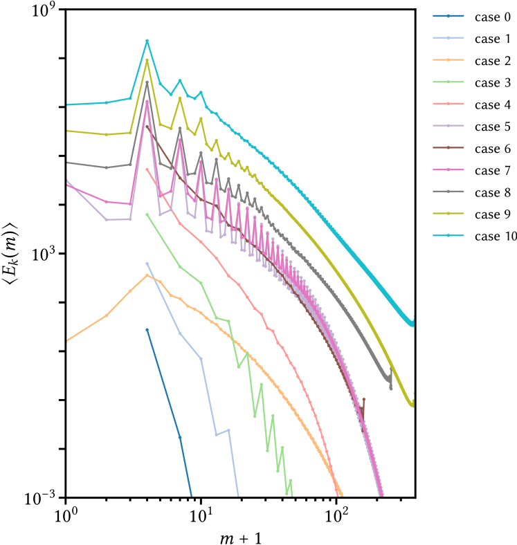
Figure 1: Time averaged kinetic energy versus azimuthal wavenumber $m$ for the 11 configurations considered in this study. Every third mode shown for clarity ($m=0,3,6,\dots$) for cases 0, 1, 3, 4 and 6. The scale on both axes is logarithmic. Note that cases 0, 1 and 3 have zero energy in the axisymmetric $m=0$ mode.

(a) Case 2, vorticity $\omega$

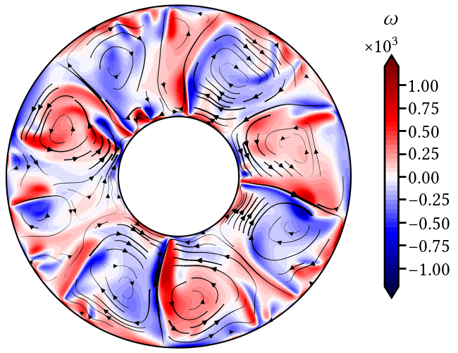
(b) Case 2, temperature $T$

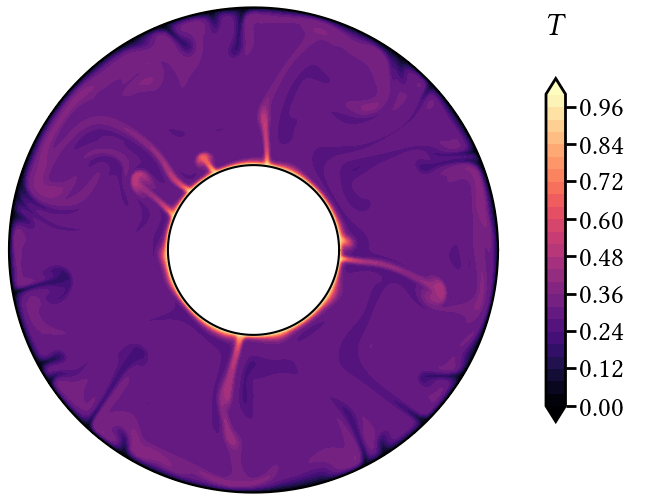
(c) Case 10, vorticity $\omega$

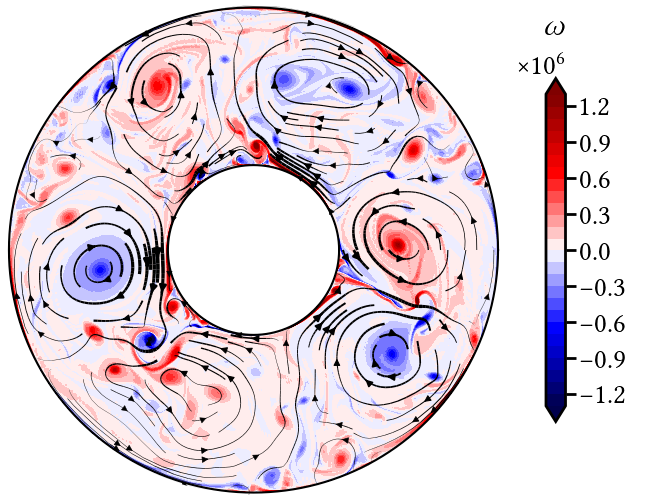
(d) Case 10, temperature $T$

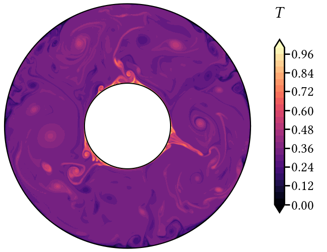
Figure 2: Solution snapshots. a: vorticity field, with superimposed velocity streamlines, for case 2 ($\mathrm{Ra}=10^{7}$, $\mathrm{Pr}=40$). b: temperature field, for case 2 and at the same discrete time. c: vorticity field, with superimposed velocity streamlines, for case 10 ($\mathrm{Ra}=10^{9}$, $\mathrm{Pr}=1$). d: temperature field, for case 10 and at the same discrete time.

We now consider in Fig. 2 a snapshot of the solution obtained for cases 2 and 10. In the latter case, the temperature field (Fig. 2d) shows three major plumes originating from the hot inner boundary, which reflect the maximum energy at $m=3$ shown in Fig. 2. Accordingly, the vorticity in Fig. 2c exhibits a large scale $m=3$ overturning circulation, with pockets of intense vorticity found in the eyes of the large-scale circulation. Note that in this set-up the plumes are anchored at the inner boundary, and that time-dependency appears mostly in the form of undulations occurring at their tip. In contrast, case 2, which corresponds to a more viscous fluid, and a lower level of forcing, is more laminar; its vorticity is notably concentrated along the edges of the large-scale convective cells (Fig. 2a). The temperature field shown in Fig. 2b appears symmetrical with regard to the top and bottom boundary layers, which are destabilized by similar cold or hot plumes displaying a mushroom head on top of a thin conduit.

3.2 Convergence analysis

Our analysis of the convergence of the 26 schemes of interest in this study follows this procedure: for each case, we compute a reference simulation using the 4th order SBDF4 IMEX multistep scheme, using a time-step size $\Delta t^{r}$ small enough in order to enable a convergence analysis that spans two orders of magnitude in terms of $\Delta t$. To equilibrate the solution prior to using $\Delta t^{r}$, we activated the possibility of a variable $\Delta t$ for the high-resolution cases. We select a time window $[t_{s},t_{e}]$ that typically covers a sizeable fraction of a convective turnover time. The reference state vector at $t=t_{s}$ is taken as the initial condition for the forward integration up to $t=t_{e}$, performed with each of the 26 schemes. The accuracy of the solution at $t=t_{e}$ is assessed using the $\mathcal{L}^{2}$ norm. For instance, the error in $\omega$ is given by

$$e_{\omega}=\sqrt{\iint_{A}[\omega(s,\varphi,t_{e})-\omega^{r}(s,\varphi,t_{e})]^{2}s\mathrm{d}s\mathrm{d}\varphi},$$

where the superscript $r$ corresponds to the reference solution. In the following, unless otherwise stated, we will systematically use this absolute definition of error.

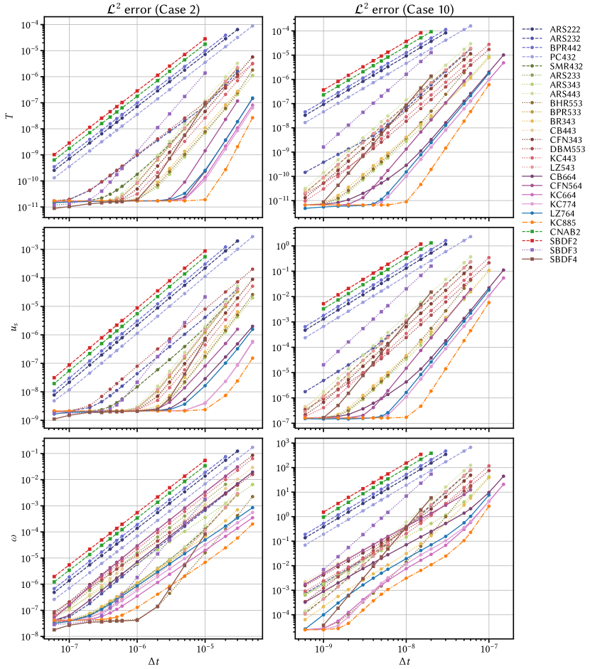
Figure 3: Convergence of the $\mathcal{L}^{2}$ error for the temperature field (top panels), the cylindrical radial velocity $u_{s}$ (middle panels) and the vorticity $\omega$ (bottom panels) for Case 2 (left column) and Case 10 (right column) as a function of the timestep size $\Delta t$. The markers correspond to the class of IMEX, with squares denoting IMEX multistep and circles IMEX-RK multistage schemes. The linestyles highlight the theoretical order with dashed lines for second order, dotted lines for third order, solid lines for fourth order and dash-dotted lines for fifth order.

We begin by a global inspection of the error behavior for the two cases we already looked at, cases 2 and cases 10, whose convergence results are shown in Figure 3. As explained above, we tried to assess the convergence properties by having at least two orders of magnitude in the range of $\Delta t$; this is sometimes barely achieved, in particular for IMEX multistep methods SBDF3 and SBDF4 whose stability domain is narrower than IMEX-RK schemes of the same order. Schemes of nominal order 2 systematically display a higher error level than schemes of order 3 and beyond, and never reach the plateau of numerical roundoff error in the range of time step sizes that we considered. Two exceptions are the ARS232 scheme by Ascher et al. (1997) and SMR432 scheme by Spalart et al. (1991) that exhibit a higher convergence rate; their convergence curves are in fact mixed with those of the schemes of nominal order 3. These schemes aside, we also note that at any given $\Delta t$ there can be a factor of $10$ difference between the worst (in this sense) order 2 scheme and the best one - PC432 is more accurate by one order of magnitude than SBDF2 or CNAB2. Order 3 schemes find themselves sandwiched between order 2 and order 4 schemes. Their convergence rate is such that the roundoff error plateau is reached for some schemes, for all fields ($T$, $u_{s}$ and $\omega$) for case 2 and all fields but the vorticity for case 10. BR343, BHR553 and ARS343 appear as the most accurate third-order IMEX-RK schemes, especially in the turbulent case 10. For the latter (ARS343) this makes sense as its explicit component is designed to match the stability properties of the RK4 scheme (Ascher et al., 1997, §2.7); see also D. For case 2, comparison of the behavior of $e_{u_{s}}$ of IMEX-RK schemes of theoretical order $3$ with that of SBDF3 highlights that some do not exhibit third-order accuracy. The 4th-order IMEX-RK schemes display overall similar error levels, below the lowest level attained by third-order schemes, this being marginally true for CFN564. For a given $\Delta t$, if one considers the temperature $T$ (Figure 3, top panel) 4th-order IMEX-RK schemes are more accurate by two orders of magnitude than the SBDF4 multistep scheme. The situation is not so clear when one considers the error in the vorticity. There SBDF4 displays a high convergence rate towards the plateau, whereas $4$th order IMEX-RK schemes do not show a clear trend. In fact, the sole scheme that appears to compete with SBDF4 is BHR553. We will return to this later. For now, we complete this preliminary overview by noting that our sole $5$th order scheme, KC885, is as expected more accurate than any other scheme considered, with the exception of SBDF4 and BHR553 being more accurate with regard to the vorticity for case $2$, over a limited range of $\Delta t$. Note finally that the fully explicit schemes that we have at our disposal (RK2 and RK4) are unstable over the range of $\Delta t$ investigated here for cases 2 and 10. This is due to the stricter limits imposed on $\Delta t$, which are such that stability coincides with reaching the numerical roundoff error plateau. Case 3 provides a configuration for which fully explicit schemes can be studied; the corresponding convergence curves are provided in C).

In summary, multistep schemes display the expected convergence rate, and an error level overall higher than IMEX-RK schemes of the same order. To get a better understanding of the error behavior across the 11 cases, we now show in Fig 4 how it evolves for the IMEX-RK KC664 scheme of Kennedy and Carpenter (2003) and the two multistep schemes SBDF2 and SBDF4. Despite the fact that the error level and admissible time step values vary across the 11 cases, we collapse the information by normalizing the error of a given scheme for a given case by its maximum value, and the timestep $\Delta t$ by the value it has when this maximum value is obtained. In addition symbols are represented such that the darker the symbol, the larger the case number. Note also that prior to collapsing the data, we got rid of those unwanted points located on a plateau, such as those present in Fig. 3 for cases 2 and 10. In the log-log representation of Fig. 4, we first observe that the behavior of SBDF2 and SBDF4 is well captured across the cases by two straight lines, of slopes 2 and 4, respectively, for the three fields of interest, $T$, $u_{s}$ and $\omega$. This illustrates nicely that they indeed conform to their expected convergence rate over the range of regimes studied. KC664, on the contrary, displays some scatter, lighter symbols (laminar cases) being overall further apart from the 4th order reference defined by SBDF4 than darker symbols (turbulent cases). This is particularly striking for the vorticity field, more moderate for $u_{s}$, and even less pronounced for $T$. For cases 9 and 10 (darker symbols) the vorticity appears to transition from 4th order to 2nd order as the value of the normalized time step decreases.

This is evidence of order reduction, to an extent that depends strongly on the regime considered.

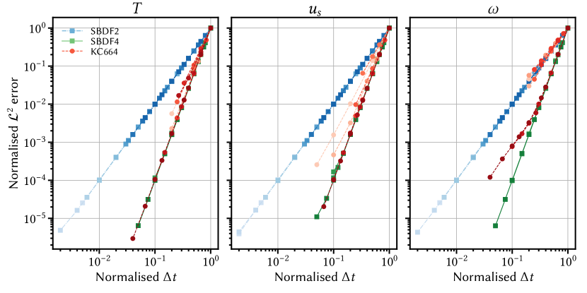
Figure 4: $\mathcal{L}^{2}$ error for $(T,u_{s},\omega)$ normalized by its maximum value (for a given case) as a function of $\Delta t$ normalized by its maximum value (for a given case too). Three schemes are considered: SBDF2, SBDF4 and KC664. The darker the color of a symbol, the higher the case number.

3.3 Order reduction

We now quantify order reduction for all cases and the 22 IMEX-RK schemes considered. To assess the order of convergence of a scheme $\mu$, we consider the two largest values of $\Delta t$ used in the convergence analysis and seek a fit for the error of the form

$$e(\Delta t)\propto\Delta t^{\,\mu},$$

with $\mu$ the sought order, that depends on the scheme and the case, and the field of interest ($T$, $u_{s}$ and $\omega$). The two largest values of $\Delta t$ are admittedly not representative of the asymptotic behavior of a scheme when $\Delta t\rightarrow 0$. Several methods display more than one scaling through the range of tested time step sizes (recall Fig. 4 above), which makes it difficult to correctly define the order of convergence. This definition of the order is not perfect, as it is biased towards runs that favor the largest integration length over accuracy, for a given number of time steps performed. The $726$ values of $\mu$ that we estimated are displayed in Figure 6.

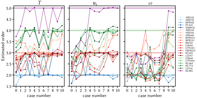
Figure 5: Measured order of convergence for the 11 cases and 22 IMEX-RK time integrators, based on the error impacting the temperature $T$ (left panel), cylindrical radial velocity $u_{s}$ (middle panel) and vorticity $\omega$ (right panel). Thick horizontal lines highlight integer values of $2$, $3$, $4$ and $5$. The 22 schemes are listed to the right, and their color reflects the theoretical order of convergence.

Figure 6: $\chi^{2}$ measure of order reduction for the 22 IMEX-RK schemes, for the temperature $T$ (left panel), cylindrical radial velocity $u_{s}$ (middle panel), and vorticity $\omega$ (right panel). A value of $0$ means no order reduction over all cases considered in this study.

To try and synthesize the information, we additionally introduce a $\chi^{2}$ measure of order reduction, defined by

$$\chi^{2}=\sum_{\mbox{\scriptsize cases}}\left(\frac{\mu^{m}-\mu^{t}}{\mu^{t}}\right)^{2},$$

where the measured order $\mu^{m}$ is set to the theoretical order $\mu^{t}$ when superconvergence is observed, i.e. when the measured order exceeds the theoretical order. Values of $\chi^{2}$ are reported in Figure 6. Figure 6 reveals that order reduction, when it affects a scheme, is more severe for $\omega$ than it is for $u_{s}$, which is itself more severe than the order reduction that impacts $T$, if it impacts $T$ at all.

Overall, we observe in Fig. 6 that IMEX-RK order 2 schemes are immune to order reduction, with SMR432 and ARS232 showing superconvergence, in particular for high Reynolds number cases. Third-order schemes show a variety of behaviors. Two schemes stand out as being particularly impacted by order reduction: CB443 and DBM553. On the contrary, BHR553 is immune to order reduction, and occasionally superconverges, as also reported by e.g. Grooms and Julien (2011). Fourth-order schemes are all prone to order reduction, especially CB664. Order reduction manifests itself mostly for our most laminar cases, from $0$ to $5$, and appears to be stronger in the most laminar cases. This phenomenon is a well-known issue that can arise due to two factors: the discrete algebraic equation (Eq. (23xag)), and the stiffness of the problem (consult Boscarino, 2007, for a thorough theoretical investigation of this issue). As previously noticed by e.g. Kennedy and Carpenter (2003) in their analysis of order reduction in a convection-diffusion-reaction problem, both differential variables ($T$, $\omega$ here) and algebraic variables ($u_{s}$ here) are impacted.

3.4 An attempt to assess the impact of the DAE on order reduction

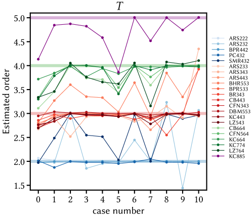
Figure 7: Measured order of convergence for the 11 cases and 22 IMEX-RK time integrators, for the simplified advection-diffusion problem whose only time-dependent variable is temperature $T$. Thick horizontal lines highlight integer values of $2$, $3$, $4$ and $5$. The 22 schemes are listed to the right, and their color reflects the theoretical order of convergence.

We try to estimate to which extent order reduction can be ascribed to the DAE by considering the reduced advection-diffusion problem

$$\frac{\partial T}{\partial t}=-\bm{\nabla}\cdot(\mathbf{u}T)+\frac{1}{Pr}\nabla^{2}T,$$ (23xdd)

subject to the same boundary conditions for temperature, and the same procedure for spatial discretization as detailed above. To cover the 11 cases investigated, we specify $\mathbf{u}$ by extracting the velocity from a random snapshot of the full problem for each case, and take the temperature field from that snapshot as the initial condition. We use this strategy in order to retain the physical properties of the solution to the full problem (in particular the level of turbulent transport) while getting rid of its algebraic component. Reference solutions to this reduced problem are produced via its time integration with the SBDF4 scheme using, again, a time step size small enough to allow convergence properties to be determined over two orders of magnitude, for each case. The temperature field $T$ is the only field that remains to evaluate accuracy and convergence properties. Estimated orders are now presented in Figure 7, noting that the findings that we present are not sensitive to the randomly chosen snapshot. Inspection of Figures 7 reveals that order reduction persists, but to a much lesser extent; there is less scatter in Fig. 7 than in the left panel of Fig. 6. In fact order reduction is now restricted to well-identified cases, namely cases 0, 5 and 7, for which the curves of Fig. 7 tend to globally dip. Schemes that exhibit occasional superconvergence (SMR432, BHR553, ARS232) do not superconverge for those cases. Schemes of order 3 and 4 that underperform for the full problem (most notably CB443, DBM553 and CB664) are now on par with other schemes of order 3 and 4. In summary, using this heuristic method of comparing orders of convergence estimated for a simplified, DAE-free problem against the full problem, we find that a significant fraction of the order reduction that impacts both differential and algebraic variables can be ascribed to the DAE.

3.5 An attempt to assess stiffness and its relationship with the observed order reduction

We now try to assess the level of stiffness of the problem we are interested in. As opposed to standard systems of ODEs for which the stiffness is set by means of an input control parameter, such as those analyzed e.g. by Boscarino and Russo (2009), in our case it is the combination of the physical control parameters ($\mathrm{Ra}$,$\mathrm{Pr}$) and the spatial properties of the 2D mesh that sets the level of stiffness, and makes its definition less straightforward.

As seen above, the differential component of the problem at hand reads schematically

$$\frac{\mathrm{d}\mathbf{x}}{\mathrm{d}t}=\mathcal{N}(\mathbf{x},\mathbf{z})+\mathcal{L}\mathbf{x},$$ (23xde)

where $\mathbf{x}$ is the differential state vector, and $\mathcal{N}$ and $\mathcal{L}$ are the nonlinear and linear operators, respectively. To estimate the stiffness we consider the ratio

$${{\color[rgb]{1,1,1}}}{\color[rgb]{0,0,0}\epsilon(t)}=\frac{\tau_{\mbox{\scriptsize L}}}{\tau_{\mbox{\scriptsize N}}(t)},$$ (23xdf)

where $\tau_{\mbox{\scriptsize N}}$ and $\tau_{\mbox{\scriptsize L}}$ are the smallest time scales associated with the nonlinear and linear terms, respectively. For Boussinesq thermal convection, nonlinearities reflect the transport of momentum and heat by fluid flow, while linearities arise from the diffusion of those same fields. The nonlinear time scale $\tau_{\mbox{\scriptsize N}}$ varies along the dynamical trajectory $\mathbf{x}(t)$. On the contrary, the linear time scale $\tau_{\mbox{\scriptsize L}}$ corresponds to the most negative real eigenvalue of $\mathcal{L}$, and is set once and for all upon prescription of the Prandtl number and the grid properties. A stiff situation occurs when $\tau_{\mbox{\scriptsize L}}\ll\tau_{\mbox{\scriptsize N}}$, or $\epsilon\ll 1$, which is a strong incentive for an implicit treatment of the linear term $\mathcal{L}\mathbf{x}$.

A first option to estimate $\tau_{\mbox{\scriptsize N}}$ and $\tau_{\mbox{\scriptsize L}}$ is to follow the logic of e.g. Grooms and Julien (2011) by writing in dimensionless form

$$\tau_{\mbox{\scriptsize N}} = \min_{\mbox{\scriptsize grid}}\left\{\frac{h_{s}}{|u_{s}|},\frac{h_{\varphi}}{|u_{\varphi}|}\right\},$$ (23xdg)

$$\tau_{\mbox{\scriptsize L}} = \frac{\mathrm{Pr}}{1+\mathrm{Pr}}\min_{\mbox{\scriptsize grid}}\left\{h_{s}^{2},h_{\varphi}^{2}\right\},$$ (23xdh)

where $\min_{\mbox{\scriptsize grid}}$ is the minimum over the physical $s-\varphi$ grid, and $h_{s}$ and $h_{\varphi}$ are the space-varying grid spacings in the $s$ and $\varphi$ directions, respectively. The nonlinear time scale is estimated based on a local measure of transport in the two directions of space, while the linear time scale assumes that the most negative eigenvalues of the linear operator correspond to an effective diffusivity equal to $\kappa+\nu$, as suggested by Eq.(24) of Grooms and Julien (2011).

We list the nonlinear and linear time scales determined for the 11 cases in the leftmost two columns of Table 4, noting that the value of $\tau_{\mbox{\scriptsize N}}$ is, for each case, the average value of $\tau_{\mbox{\scriptsize N}}(t)$ found for $5$ independent snapshots. The corresponding stiffness parameter, $\epsilon_{\tau}$, spans a moderate range of two decades. The increase of turbulence and reduction of $\tau_{\mbox{\scriptsize N}}$ goes alongside an increase in the resolution that induces a concomitant decrease of $\tau_{\mbox{\scriptsize L}}$. We are in what authors currently refer to as an intermediate range of stiffness (Kennedy and Carpenter, 2019), that can indeed be detrimental to the order of convergence of some IMEX-RK methods.

Case	$\tau_{\mbox{\scriptsize N}}$	$\tau_{\mbox{\scriptsize L}}$	$\epsilon_{\tau}$	$\epsilon_{\Delta t}$	$\epsilon_{\lambda}$	$\epsilon_{\lambda}$ (red.)
0	9.14 $10^{-3}$	2.06 $10^{-6}$	2.22 $10^{-4}$	1.97 $10^{-4}$	2.84 $10^{-4}$	2.92 $\mathbf{10^{-4}}$
1	8.92 $10^{-4}$	6.23 $10^{-7}$	6.99 $10^{-4}$	8.14 $10^{-4}$	1.69 $10^{-3}$	1.05 $10^{-3}$
2	5.99 $10^{-5}$	1.40 $10^{-9}$	2.34 $\mathbf{10^{-5}}$	3.66 $\mathbf{10^{-5}}$	3.50 $\mathbf{10^{-5}}$	1.40 $10^{-3}$
3	1.55 $10^{-4}$	1.93 $10^{-7}$	1.25 $10^{-3}$	2.99 $10^{-3}$	4.28 $10^{-3}$	2.65 $10^{-3}$
4	1.85 $10^{-5}$	3.74 $10^{-8}$	2.02 $10^{-3}$	3.59 $10^{-3}$	5.93 $10^{-3}$	4.97 $10^{-3}$
5	1.07 $10^{-5}$	9.42 $10^{-9}$	8.78 $10^{-4}$	7.94 $10^{-4}$	1.36 $10^{-3}$	4.27 $10^{-4}$
6	4.10 $10^{-6}$	1.17 $10^{-8}$	2.86 $\mathbf{10^{-3}}$	6.13 $\mathbf{10^{-3}}$	9.18 $\mathbf{10^{-3}}$	7.99 $\mathbf{10^{-3}}$
7	1.39 $10^{-6}$	5.71 $10^{-10}$	4.10 $10^{-4}$	6.87 $10^{-4}$	6.98 $10^{-4}$	2.80 $10^{-4}$
8	7.42 $10^{-7}$	7.20 $10^{-10}$	9.71 $10^{-4}$	3.04 $10^{-3}$	3.54 $10^{-3}$	3.47 $10^{-3}$
9	2.26 $10^{-7}$	2.32 $10^{-10}$	1.03 $10^{-3}$	2.05 $10^{-3}$	1.78 $10^{-3}$	1.06 $10^{-3}$
10	1.35 $10^{-7}$	1.41 $10^{-10}$	1.05 $10^{-3}$	1.57 $10^{-3}$	3.82 $10^{-3}$	4.14 $10^{-3}$

Table 4: Three different estimates of the stiffness of the problem at hand, for all cases considered in this study. The rightmost column gives an estimate of stiffness for the problem reduced to the advection–diffusion equation for temperature. Bold face fonts used for largest and smallest values. See text for details.

Our second estimate of stiffness compares the maximum time-step allowed for stable computation using the ARS343 IMEX-RK method, $\Delta t_{\mbox{\scriptsize max}}^{{\mbox{\scriptsize imex}}}$, with the maximum time step $\Delta t_{\mbox{\scriptsize max}}^{{\mbox{\scriptsize expl}}}$ allowed if one resorts to the fully explicit RK4 integrator. By considering the ratio

$$\epsilon_{\Delta t}=\frac{\Delta t_{\mbox{\scriptsize max}}^{{\mbox{\scriptsize expl}}}}{\Delta t_{\mbox{\scriptsize max}}^{{\mbox{\scriptsize imex}}}},$$

we have an estimate of the stiffness based on an indirect probing of the stability regions of the timeschemes considered. As a matter of fact, the IMEX-RK scheme chosen here is ARS343 because the stability region of its explicit component matches by design that of RK4 (Ascher et al., 1997, §2.7); therefore we should not expect an offset of $\epsilon_{\Delta t}$ by an unwanted factor. Values of $\epsilon_{\Delta t}$ are tabulated alongside values of $\epsilon_{\tau}$ in Table 4. They fall within a factor of $3$ within the values of $\epsilon_{\tau}$, in a non-systematic way.

The third and final option we consider is to investigate directly the eigenvalues of the operators at hand. In the vicinity of a point $\mathbf{x}^{\star}(t^{\star})$, we approximate $\mathcal{N}$ by its tangent linear operator $\mathcal{N}^{\prime}$ such that

$$\mathcal{N}(\mathbf{x}^{\star}+\delta\mathbf{x})=\mathcal{N}(\mathbf{x}^{\star})+\mathcal{N}^{\prime}(\mathbf{x}^{\star})\delta\mathbf{x}.$$ (23xdu)

Under these circumstances, if we define $\mathcal{Q}(\mathbf{x}^{\star})=\mathcal{N}^{\prime}(\mathbf{x}^{\star})+\mathcal{L}$, the behavior of the solution in the vicinity of $\mathbf{x}^{\star}$ obeys

$$\frac{\mathrm{d}\delta\mathbf{x}}{\mathrm{d}t}=\mathcal{Q}(\mathbf{x}^{\star})\delta\mathbf{x}.$$ (23xdv)

For each case, we constructed a two-dimensional, second-order finite-difference approximation of $\mathcal{Q}(\mathbf{x}^{\star})$, upon the Chebyshev–Fourier grid used in our spatial approximation. We did so in order to obtain a sparse, 2D, operator amenable to eigenvalue analysis for both full and reduced problems. The full problem, though, was approximated using a formulation based on the streamfunction alone (see e.g. Canuto et al., 2007, §1.4), in order to facilitate its implementation. We benchmarked our finite difference approximation by computing the critical parameters for convection, with a critical wavenumber $m_{\mbox{\footnotesize crit}}=3$ and Rayleign number $\mathrm{Ra}_{{\mbox{\footnotesize crit}}}=1768$ (recall section 3.1). To obtain the eigenvalues of $\mathcal{Q}(\mathbf{x}^{\star})$, we resorted to the sparse library of the scientific python package Scipy (Virtanen et al., 2020), in conjunction with the SLEPc toolbox for python (Hernandez et al., 2005; Dalcin et al., 2011). Cases of modest resolution lend themselves to the full calculation of the spectrum, and the example of case 3 is given in Figure 8. We observe that the distribution of eigenvalues is symmetrical with respect to the real axis, and that eigenvalues are concentrated in the vicinity of the origin, at the exception of a few purely real values that are quite distant, and correspond to the inverse value of the diffusive time scale on the smallest grid spacing, of non-dimensional value ${\pi^{2}/N_{s}^{4}}$. These negative eigenvalues of large magnitude are due to the linear component of the problem at hand, and the ones responsible for stiffness. We associate the eigenvalues of largest imaginary part with the advective component of $\mathcal{Q}$, and therefore the reciprocal value of $\tau_{\mbox{\scriptsize N}}$.

Figure 8: Eigenvalues $\lambda$ of the tangent linear operator computed for case 3, for the full problem and the reduced problem restricted to the heat equation considered alone. Left: full spectrum. Right: zoom in the vicinity of the origin, in the region of the complex plane defined by the dashed rectangle in the left panel.

For cases of larger size (for case 10 the size of the sparse matrix to deal with is $878206\times 878206$) we computed only the 100 eigenvalues of largest negative real parts, $\lambda^{r}$, and 100 eigenvalues of largest imaginary parts, $\lambda^{i}$. Our estimate of stiffness is given by

$$\epsilon_{\lambda}=\frac{\max{\Im({\lambda^{i}})}}{\max{|\Re({\lambda^{r}})|}},$$ (23xdw)

in which $\Im()$ is the imaginary part. For this calculation, we used the same 5 independent snapshots for each case as the ones used to estimate $\epsilon_{\tau}$. Results are listed in Table 4, and are in agreement, again within a factor of $3$ with estimates based on $\epsilon_{\tau}$ and $\epsilon_{\Delta t}$. The three estimates of $\epsilon$ point to case 6 as being the least stiff, even though the stiffness parameter does not exceed $10^{-2}$. Case 6 had a Prandtl number of unity, which implies that the diffusivities of heat and momentum are equal. The stiffest case is case 2, which has $\mathrm{Pr}=40$. For case 2, a relatively large resolution is needed to resolve the small-scale temperature anomalies within a pretty laminar flow (recall Figures 2a and 2b). Table 4 also comprises values of $\epsilon_{\lambda}$ computed for the reduced problem (advection-diffusion equation of temperature with a prescribed flow), that we used previously to try and assess the impact of the DAE on the observed order reductions. The values of $\epsilon_{\lambda}$ for the reduced problem are consistent with those found for the complete problem, with one exception. In this simplified system, case 6 remains the least stiff case, and it is now the barely supercritical case 0 that is the stiffest case. Case 2 ceases to be the stiffest case, since its most negative eigenvalues are associated with the diffusion of momentum, not heat. Accordingly, the value of $\epsilon_{\lambda}$ we find for the reduced case 2 is precisely multiplied by a factor of $\mathrm{Pr}=40$, compared with the value found for the full problem. This increase is not seen in the three cases that have $\mathrm{Pr}$ below unity (5, 7 and 9), for which the largest negative eigenvalues remain connected with the diffusion of heat.

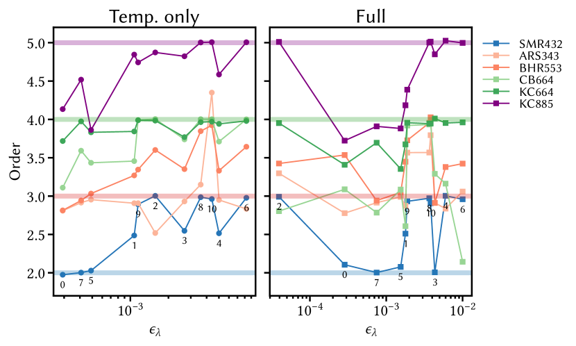
Figure 9: Order of convergence for the temperature field $T$, in the reduced problem set-up (left panel), and for the full problem (right panel), as a function of the stiffness parameter $\epsilon_{\lambda}$ estimated for each problem for all 11 cases and for some selected time schemes. See text for details. $\epsilon_{\lambda}$ sur

We conclude the analysis of the impact of stiffness by showing the measured order of convergence for the reduced, DAE-free, and full problems against the corresponding values of $\epsilon_{\lambda}$ in figure 9, with the hope that this representation will get rid of the jaggedness of figures 6 (left panel) and  7. Within the modest range of $\epsilon_{\lambda}$ that our investigations enabled, we observe in Fig. 9, left panel, that for the reduced problem, KC774, CB664 and KC885 are close to meeting their expected order of convergence for $\epsilon_{\lambda}\gtrsim 10^{-3}$. SMR432 exhibits an order of convergence larger than 2 for $\epsilon_{\lambda}\gtrsim 10^{-3}$ as well. ARS343 superconverges only for case 10, while BHR553 superconverges for all cases but case 0. This scheme is by design supposed to be immune to order reductions caused by stiffness and the DAE (Boscarino and Russo, 2009). For the full problem, the range of $\epsilon_{\lambda}$ covered is a bit broader, and we find it noteworthy that for the stiffest case 2, order is restored. In fact, the curves we obtain in particular for schemes KC774 and KC885 show a reasonable similarity with the curves obtained for those same schemes applied to Kap’s problem by their genitors Kennedy and Carpenter (2019).

In summary, we think that the stiffness of the cases we considered in this study covers a moderate, intermediate range of values spanning slightly less than two decades for the reduced problem and two and a half decades for the full Boussinesq convection problem. We find that even if stiffness has an impact on the convergence of some schemes over a limited range, typically $10^{{\color[rgb]{0,0,0}-4}}\lesssim\epsilon_{\lambda}\lesssim 10^{-3}$ for the stiffness parameter we determined, it is mostly the DAE that causes the degradation of convergence. The reduction in order affects both differential and algebraic variables, probably by virtue of the coupling induced by the equations of the problem at hand. Yet, schemes of theoretical order 2 are not affected by order reduction. Higher-order time integrators that are by design immune to such problems, such as BHR553 or the IMEX multistage methods, may appear as the schemes of choice.

This statement remains to be weighted against a measure of the stability and computational efficiency of those schemes, which is the topic of the next subsection.

3.6 Stability and computational efficiency

The explicit treatment of nonlinearities imposes a restriction on the available time step that is subject to a time-dependent Courant-Friedrich-Levy condition

$$\Delta t\leq\alpha_{\mbox{\scriptsize\sc cfl}}\min_{\mbox{\scriptsize grid}}\left\{\frac{h_{s}}{|u_{s}|},\frac{h_{\varphi}}{|u_{\varphi}|}\right\},$$

where the $\mathcal{O}(1)$ prefactor $\alpha_{\mbox{\scriptsize\sc cfl}}$ depends on the time integrator and the case considered. In order to determine empirically the maximum admissible value of $\alpha_{\mbox{\scriptsize\sc cfl}}$, $\alpha^{\mbox{\scriptsize\sc max}}_{\mbox{\scriptsize\sc cfl}}$, for the $11\times 26$ combinations of this study, we followed Gastine (2019) and inspected the timeseries of viscous dissipation $D_{\nu}(t)$ and its fluctuations for different values of $\alpha_{\mbox{\scriptsize\sc cfl}}$. The maximum admissible value of $\alpha_{\mbox{\scriptsize\sc cfl}}$, $\alpha^{\mbox{\scriptsize\sc max}}_{\mbox{\scriptsize\sc cfl}}$ is determined to $0.02$ accuracy by requesting that the timeseries of $D_{\nu}(t)$ does not exhibit any flagrant spike, over a time window of width roughly equal to 5 convective turnover times; the time window is case-dependent, but for a given case, it is the same for all time integrators. Figure 10a illustrates this methodology for case 9 and the ARS343 scheme, a configuration for which we find $\alpha^{\mbox{\scriptsize\sc max}}_{\mbox{\scriptsize\sc cfl}}=1.10$. This arguably tedious methodology is meant at preserving the accuracy of the solution, and can not lead to the disturbing occurrence of stable yet inaccurate IMEX-RK schemes reported by Grooms and Julien (2011), and mentioned in the introduction. In this regard, our estimate of $\alpha^{\mbox{\scriptsize\sc max}}_{\mbox{\scriptsize\sc cfl}}$ is conservative. We refer readers interested in a more standard assessment of stability and efficiency to appendix E, where we report accuracy versus runtime for cases 2 and 10.

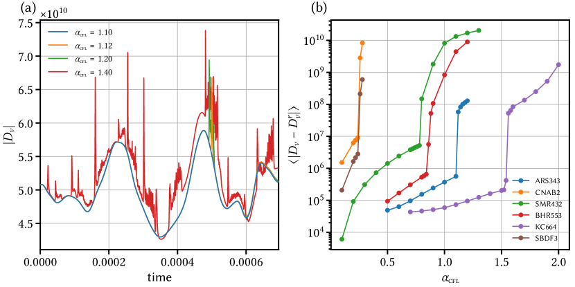
Figure 10: a: Time series of viscous dissipation $|D_{\nu}|$ for case 9 advanced with the ARS343 IMEX-RK scheme, considering various values of $\alpha_{\mbox{\scriptsize\sc cfl}}$. The highest admissible value we find in this setup is $\alpha_{\mbox{\scriptsize\sc cfl}}=1.10$. b: Time average of $|D_{\nu}-D_{\nu}^{r}|$ as a function of $\alpha_{\mbox{\scriptsize\sc cfl}}$ for case 9 and 6 time integrators. $D_{\nu}^{r}(t)$ is a reference time series for viscous dissipation obtained with the SBDF4 time scheme. Note that the scale on the $y$-axis is logarithmic. For a scheme, the maximum admissible value of $\alpha_{\mbox{\scriptsize\sc cfl}}$ is the largest one that precedes the steep increase in the curve.

We now propose an automated way of reaching the same conclusions. We begin by establishing a master curve for $D_{\nu}(t)$ over the interval of interest using the SBDF4 time scheme and the smallest $\alpha_{\mbox{\scriptsize\sc cfl}}$. This master curve is denoted by $D_{\nu}^{r}(t)$ where again, the superscript $r$ stands for reference. Given the $D_{\nu}(t)$ computed for an integrator and a value of $\alpha_{\mbox{\scriptsize\sc cfl}}$, we evaluate the time average of $|D_{\nu}-D_{\nu}^{r}|$ over the window of interest using splines for the numerical integration. As an example, we show $\langle|D_{\nu}-D_{\nu}^{r}|\rangle$ in Figure 10b for case 9 and 6 schemes. We observe a sharp transition in the behavior of this quantity, for relatively low values of $\alpha_{\mbox{\scriptsize\sc cfl}}$ for the two multistep schemes (CNAB2 and SBDF3) and larger values for the IMEX-RK schemes. The largest value of $\alpha_{\mbox{\scriptsize\sc cfl}}$ before the transition matches the $\alpha^{\mbox{\scriptsize\sc max}}_{\mbox{\scriptsize\sc cfl}}$ obtained by visual inspection of the timeseries of $D_{\nu}(t)$.

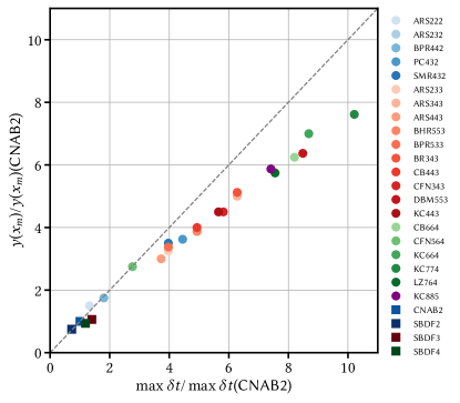
Figure 11: Ratio of the maximum ordinate of the stability curve of the explicit component of a time integrator to that of the CNAB2 scheme as a function of the ratio of the maximum timestep size admissible to the maximum time step admissible for CNAB2. The case considered is case 10 ($\mathrm{Re}=13320$, stiffness parameter $\epsilon\sim 3\times 10^{-3}$). The dashed grey line is the prediction based on Eq. (23xdy).

The value of $\alpha^{\mbox{\scriptsize\sc max}}_{\mbox{\scriptsize\sc cfl}}$ can be converted into a maximum attainable value of the time step size, $\Delta t^{\mbox{\scriptsize\sc max}}$: we take it to be the average $\Delta t$ obtained in the same setups that led to the determination of $\alpha^{\mbox{\scriptsize\sc max}}_{\mbox{\scriptsize\sc cfl}}$, meaning that we find $26$ values of $\Delta t^{\mbox{\scriptsize\sc max}}$ (one per scheme) per case. In those cases where nonlinearities dominate, with stiffness parameters $\epsilon$ of the order of $10^{-2}$ (recall Table 4 above), it is actually possible to make a decent guess of $\Delta t^{\mbox{\scriptsize\sc max}}$ based on the boundary of the stability region of the explicit component of the scheme under scrutiny. This stability region is bounded by a curve that mostly lies in the left hand side of the complex plane, that of negative real parts. We anticipate that in moderately stiff situations where nonlinearities play a major part in the dynamics, it is this curve that will control the stability of the implicit explicit scheme, even if it does not correspond to the stability curve of the combined scheme, as studied by e.g. Karniadakis et al. (1991) and Izzo and Jackiewicz (2017) for test problems. As discussed above in our analysis of stiffness, transport will effectively probe the eigenvalues of the semi-discrete tangent linear operator with the largest imaginary parts (in absolute value). Let $\lambda_{m}$ denote the eigenvalue of largest imaginary part. As a rule of thumb we want $\lambda_{m}\Delta t$ to be close to the stability curve. For transport-dominated physics, we thus make the tentative prediction that for any scheme

$$\Delta t^{\mbox{\scriptsize\sc max}}\mbox{ (scheme) }=f\times y(x_{m})\mbox{ (scheme) },$$ (23xdx)

where the factor $f$ is a function of the spatial discretization only, $x_{m}=\Re({\lambda_{m}}\Delta t)$ and the ordinate $y(x_{m})$ on the stability curve can be determined numerically. These curves are provided in D for completeness. If this equality holds, provided we know $\Delta t^{\mbox{\scriptsize\sc max}}$ of a case for one scheme (CNAB2, say) we may expect that

$$\Delta t^{\mbox{\scriptsize\sc max}}\mbox{ (scheme) }=\frac{y(x_{m})\mbox{(scheme)}}{{y(x_{m})\mbox{(CNAB2)}}}\,\,\Delta t^{\mbox{\scriptsize\sc max}}\mbox{ (CNAB2) }.$$ (23xdy)

The relevance of this line of reasoning is shown in Figure 11 where this empirical prediction is compared with the measured value for case 10, our most turbulent case. We find that the overall trend is that the prediction slightly overestimates the actual value, typically by within 10 to 20 %. Figure 11 highlights the fact that the most stable order 3 scheme is DBM553, a result that can be understood by inspection of the stability region of its explicit component given in Figure 15, middle panel. Of all the third order schemes we considered, DBM553 has the most elongated region of stability in the vicinity of the $y$-axis of the complex plane. In fact, it was designed for the very purpose of accommodating the constraint on the available time step size arising from the location of eigenvalues of the explicit component of a model being located along the imaginary axis (Kinnmark and Gray, 1984). A closer inspection of the IMEX-RK schemes which share the same stability domain for their explicit component reveals very similar CFL coefficients for case 10 with for instance $\alpha^{\mbox{\scriptsize\sc max}}_{\mbox{\scriptsize\sc cfl}}(\text{ARS232})=0.54$ and $\alpha^{\mbox{\scriptsize\sc max}}_{\mbox{\scriptsize\sc cfl}}(\text{SMR432})=0.56$; or $\alpha^{\mbox{\scriptsize\sc max}}_{\mbox{\scriptsize\sc cfl}}(\text{ARS343})=0.8$ and $\alpha^{\mbox{\scriptsize\sc max}}_{\mbox{\scriptsize\sc cfl}}(\text{BR343})=0.82$. This is another indication that the stability domain of the explicit part only provides a decent estimate of the actual stability of an IMEX-RK scheme in the limit of advection-dominated flows. To conclude this paragraph, we note that for cases of more dramatic stiffness, one should probably consider the stability region of the complete IMEX scheme, an endeavor that we did not pursue.

To evaluate the efficiency of a given scheme, we consider the following ratio

$$\mbox{eff}=\frac{\alpha^{\mbox{\scriptsize\sc max}}_{\mbox{\scriptsize\sc cfl}}}{\mbox{cost}},$$ (23xdz)

where cost refers to the amount of work required to advance the solution by one time step $\Delta t$. In practice cost is the average cpu time measured over $1000$ iterations using reproducible runtime conditions (same compute nodes, exclusive access to the compute node, one single OpenMP thread). Note that the linear matrix solves amount for the majority of the walltime, and hence the number of solves per iteration $n^{I}$ in Table 1 provides a decent estimate of the actual relative walltime. We evaluated the efficiency of the 26 schemes considering the 11 cases. We investigate how the gain one may obtain in terms of a larger $\alpha^{\mbox{\scriptsize\sc max}}_{\mbox{\scriptsize\sc cfl}}$ using an IMEX-RK scheme trades off with the extra operations that are needed. (Again, at this stage, we do not consider the benefit in terms of accuracy.) Given the popularity of the CNAB2 integrator in our community, we normalize the efficiency by the efficiency of CNAB2. Results are displayed in Figure 13 for cases, 2, 5 and 10 that have $\mathrm{Re}=26$, $513$ and $13320$, respectively, and whose stiffness parameter $\epsilon$ we estimated in section 3.5 to be $\sim 3\times 10^{-5}$, $\sim 10^{-3}$ and $\sim 3\times 10^{-3}$, respectively.

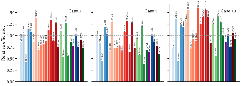
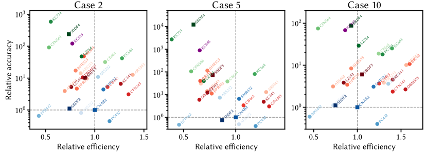
Figure 12: Efficiency of the time integrators relative to the efficiency of CNAB2 for cases 2, 5 and 10 from left to right. Horizontal dashed lines correspond to a value of unity. See text for details.

Figure 13: Efficiency and accuracy of the time integrators relative to the efficiency and accuracy of CNAB2 for cases 2, 5 and 10 from left to right. The scale on the $y$-axis is logarithmic. See text for details. Horizontal and vertical dashed lines correspond to a value of unity.

Relative efficiency is in all cases bounded between $0.5$ and $1.50$. We observe that the number of IMEX-RK schemes that outperform CNAB2 increases dramatically with the Reynolds number from 5 for Case 2 to 14 for case 10. For the latter, the 14 schemes comprise 3, 7 and 4 schemes of order 2, 3 and 4, respectively. This indicates that the gain in stability in transport-dominated regimes outweigh the increase in the number of operations as the resolution increases. For case 10, we note a relative grouping of multistep schemes around 1, with SBDF3 being slight more efficient than CNAB2, in agreement with its more elongated stability domain close to the imaginary axis (D). A scheme that appears to be consistently efficient across the 3 cases is ARS343. The DBM553 scheme by Vogl et al. (2019) and the BR343 scheme by Boscarino and Russo (2007) transition from a poor efficiency in the laminar case 2 to an excellent one in the turbulent case 10.

3.7 Trade-off between accuracy and efficiency

We now weigh efficiency and accuracy for recommendations to be made to the practitioner. The accuracy is characterized by the error one expects for a simulation performed at the maximum available time step size, $\Delta t^{\mbox{\scriptsize\sc max}}$, as defined in the previous section. This error is computed based on the scaling of the error on temperature with $\Delta t$ that can be obtained for the various convergence curves introduced in section 3.2 above, by taking $\Delta t=\Delta t^{\mbox{\scriptsize\sc max}}$. Therefore, our target practitioner wishes to integrate the solution for the longest time span possible given his/her computing resources with the hope that the error will remain as small as possible. We normalize the error with the error estimated for CNAB2 and show in Figure 13 where the various schemes considered in this work are located in the (relative efficiency, relative error) plane for cases 2, 5 and 10 again.

Schemes located in the top right quadrant of each panel are more accurate and yet more efficient than CNAB2. Six IMEX-RK schemes are systematically located in this quadrant, one scheme of order 2, SMR432 (Spalart et al., 1991), four schemes of order 3, ARS343 (Ascher et al., 1997), CB443 (Cavaglieri and Bewley, 2015), CFN343 (Calvo et al., 2001), KC443 (Kennedy and Carpenter, 2003) and one scheme of order 4, KC664 (Kennedy and Carpenter, 2003). At the operational, dissipation-based limit of stability, it is remarkable to note that ARS343 and KC664 enable a significant improvement of accuracy at a lower cost, regardless of the configuration. In the turbulent regime, where the explicit components of time integrators prevail, CNAB2 is outperformed by no less than 14 schemes, which include 2 schemes of order 2, 8 schemes of order 3 (including SBDF3), and 4 schemes of order 4.

4 Summary and recommendations

We have applied 22 multistage, 4 multistep implicit-explicit, and 2 fully explicit integrators to the problem of Boussinesq thermal convection in a two-dimensional cylindrical annulus, over a broad range of regimes whose exploration was made possible by the definition of 11 different physical setups. Our spatial discretization rests on a pseudo-spectral collocation method applied to the vorticity streamfunction formulation of the problem. We summarize our findings as follows:

• Over the range of cases considered, IMEX multistep methods exhibit their expected order of convergence. IMEX-RK methods of second order also show the expected convergence. Some IMEX-RK methods of order 3 and 4 show order reduction, that affect both the algebraic and differential variables of the chosen formulation.

• We have attempted to evaluate the stiffness of the cases using three different strategies that lead to the same conclusion: the small parameter that quantifies stiffness, $\epsilon$, covers a moderate and intermediate range of values spanning two and a half decades for the full Boussinesq convection problem, between $3\times 10^{-5}$ and $10^{-2}$.

• We find that even if stiffness has an impact on the convergence of some schemes over a limited range of $\epsilon$, typically $10^{-4}\lesssim\epsilon\lesssim 10^{-3}$, it is mostly the discrete algebraic equation that causes the degradation of convergence. The reduction in order affects both differential and algebraic variables, probably by virtue of the coupling induced by the equations of the problem at hand.

• IMEX-RK time integrators that are by design immune to such problems, such as BHR553 (Boscarino and Russo, 2009), exhibit nominal convergence properties, or even better-than-nominal properties in the least stiff (transport-dominated) situations.

• We have defined the efficiency of a scheme by the ratio of the maximum admissible value of the Courant number, $\alpha^{\mbox{\scriptsize\sc max}}_{\mbox{\scriptsize\sc cfl}}$, divided by the cost of performing one time step. By maximum admissible value we understand a value that generates a smooth timeseries of viscous dissipation within the system. Viscous dissipation is a demanding quantity, whose behavior help us define an acceptable (or not acceptable) solution. With this at hand, we have reported the efficiency of the schemes relative to the popular CNAB2 for 3 cases that we consider representative. We found that the relative efficiency was bounded between $0.5$ and $1.5$. Also, CNAB2 is not the method of choice when going to transport-dominated cases, as no less than 14 schemes are more efficient than CNAB2 for our most turbulent case.

• This last statement becomes even stronger when relative accuracy is added to the analysis. By relative accuracy here we mean the ratio of the error anticipated for a scheme running at the operational, dissipation-based limit of stability, whose expected error can be estimated based on the convergence analysis, to the same error anticipated for CNAB2 at its limit of stability (and that for each case). For the same three representative cases, we find that $6$ schemes combine the assets of being less expensive and more accurate than CNAB2: SMR432 (Spalart et al., 1991), CFN343 (Calvo et al., 2001), ARS343 (Ascher et al., 1997), CB443 (Cavaglieri and Bewley, 2015), KC443 and KC664 (Kennedy and Carpenter, 2003).

• For the problem of thermal convection in a cylindrical annulus with a spectral discretization in space, it appears that the default integrator should be the third-order ARS343, or possibly KC664 if higher accuracy is sought.

For turbulent cases, or in more general terms, transport-dominated cases, the performance of an implicit-explicit scheme is dictated by its explicit component, as the part treated explicitly here is purely advective. The previous general recommendation can be amended on a case-by-case basis: for instance the third-order scheme  DBM553 proposed by Vogl et al. (2019) may well prove superior to any third-order scheme for turbulent transport-dominated 2D problems reaching $\mathrm{Re}\sim 10^{5}$ and beyond. In fact, on this path, provided $\epsilon\sim 1$ is reached, RK4 may well prove competitive, even more so if a regridding is performed to alleviate the stringent time step limitations due to the clustering of grid points near the boundaries, as done e.g. by Johnston and Doering (2009) using the mapping proposed by Kosloff and Tal-Ezer (1993).

Before discussing a tentative extrapolation of our results to three-dimensional geometry, we should add the following important caveat: stiffness in our setup is controlled by the most negative real eigenvalues of the linear part that is treated implicitly, and our recommendations may not be suited for those problems where stiffness comes from fast waves, i.e. large imaginary eigenvalues of the linear terms.

Three-dimensional problems concerned with the modeling of planetary interiors in global spherical geometry are nowhere near reaching values of $\mathrm{Re}$ as extreme as $10^{6}$. Recent parametric studies of convection-driven dynamo in a spherical shell geometry by Schwaiger et al. (2019), Gastine et al. (2020) and Tassin et al. (2021) have values of $\mathrm{Re}$ in the range $100-3000$, while single-case, rapidly-rotating trophy studies by Schaeffer et al. (2017); Sheyko et al. (2018) (DNS) and Aubert (2019) (LES) report $\mathrm{Re}\sim 5000$ and $\mathrm{Re}\sim 20000$ for the DNS and LES, respectively. We may wonder how our findings can carry over to these simulations. In F, we attempt to convert our 2D tradeoff diagrams into their 3D counterparts, by making the strong assumptions that accuracy and stability remain the same, i.e. that the convergence properties and values of $\alpha^{\mbox{\scriptsize\sc max}}_{\mbox{\scriptsize\sc cfl}}$ are not affected. The sole impact of the change of geometry that factor in the analysis lies in the cost, where we acknowledge that in a three-dimensional pseudo-spectral code of planetary core dynamics, explicit stages are the most expensive steps in a calculation, as there is no efficient equivalent of the fast Fourier transform for the Legendre transform. Taking this into account, non globally stiffly accurate IMEX-RK schemes, that require an extra assembly stage, are penalized compared with stiffly accurate ones.

For the range of $\mathrm{Re}$ typical of recent parametric studies, and under the strong assumptions that we made, we predict that the schemes of choice for $\mathrm{Re}\sim 1000$ in three dimensions should be PC432 (order 2), ARS343 and BPR533 (order 3) and KC664 (order 4). Relative to the classic CNAB2, these schemes should yield a reduction of the time to solution while enabling more accurate solutions. This analysis ignores the memory imprint of the schemes (recall Tab. 1) , as the codes in question are massively parallel and should be immune to this issue, at least for the level of $\mathrm{Re}$ considered. If the level of turbulence should increase for 3D simulations, then we anticipate again that it is the robustness and efficiency of the explicit component of IMEX schemes that will matter. Also, depending on the problem studied, hybrid splitting strategies, that would treat explicitly some linear terms with the aim of increasing the efficiency of the calculation, look like an interesting avenue for investigation, especially in turbulent situations. Also worth investigating are the IMEX general linear method (GLM) that have recently come to the fore. They appear to overcome some of the inherent limitations of IMEX-RK schemes, such as order reduction. Zhang et al. (2016) for instance explored several IMEX strategies to compute 2-D and 3-D simulations of thermal rising bubbles (Giraldo and Restelli, 2008) and showed that the IMEX-GLM were immune to order reduction and exhibited the best accuracy/efficiency tradeoff among the tested schemes (see their Fig. 10). We conclude by hoping that our findings will serve as an incentive for the community of stars and planetary fluid interiors modelers to transition towards IMEX-RK integrators, which possess the extra convenient property of being self-restarting (their initialization only requires knowledge of the current state vector), regardless of their order of accuracy.

Appendix A Multistep schemes

We provide the reader with the vectors of coefficients $\mathbf{a}$, $\mathbf{b}$ and $\mathbf{c}$ for CNAB2, SBDF2, SBDF3 and SBDF4. These vectors define a linear multistep method with $K$ steps according to

$$\left(1-\Delta tc_{-1}\mathcal{L}\right)\mathbf{x}_{i+1}=\sum^{K-1}_{j=0}\left[a_{j}\mathbf{x}_{i-j}+\Delta tb_{j}\mathcal{N}(\mathbf{x}_{i-j})+\Delta tc_{j}\mathcal{L}\mathbf{x}_{i-j}\right],$$ (23xea)

where $c_{-1}\neq 0$. Table 5 enlists these three vectors when a fixed time step size $\Delta t$ is used (see e.g. Peyret, 2002, Table 4.4).

Table 5: Coefficients of the multistep schemes considered in this study when a fixed time step size $\Delta t$ is employed.

method	$K$	$\mathbf{a}$	$\mathbf{b}$	$\mathbf{c}$
CNAB2	2		$[3/2,-1/2]$	$[1/2,1/2,0]$
SBDF2	2	$[4/3,-1/3]$	$[4/3,-2/3]$	$[2/3,0,0]$
SBDF3	3	$[18/11,-9/11,2/11]$	$[18/11,-18/11,6/11]$	$[6/11,0,0,0]$
SBDF4	4	$[48/25,-36/25,16/25,-3/25]$	$[48/25,-72/25,48/25,-12/25]$	$[12/25,0,0,0,0]$

Following Wang and Ruuth (2008), those vectors can be generalised to the case of variable time step sizes. In the following, we define

$$\Delta t_{i}=t_{i}-t_{i-1},$$

and the ratio

$$\delta_{i}=\dfrac{\Delta t_{i}}{\Delta t_{i-1}}\,.$$

For the different IMEX multistep schemes considered here, we then obtain:

• CNAB2

  $$\mathbf{b}=\left[1+\dfrac{1}{2}\delta_{i},-\dfrac{1}{2}\delta_{i}\right],\ \mathbf{c}=\left[\dfrac{1}{2},\dfrac{1}{2}\right],$$

• SBDF2

  $$\mathbf{a}=\left[\dfrac{(1+\delta_{i})^{2}}{1+2\delta_{i}},-\dfrac{\delta_{i}^{2}}{1+2\delta_{i}}\right],\ \mathbf{b}=\left[\dfrac{(1+\delta_{i})^{2}}{1+2\delta_{i}},-\dfrac{(1+\delta_{i})\delta_{i}}{1+2\delta_{i}}\right],\ \mathbf{c}=\left[\dfrac{1+\delta_{i}}{1+2\delta_{i}},0,0\right],$$

• SBDF3

  $$\mathbf{a} =\dfrac{1}{\alpha}\left[\dfrac{(1+\delta_{i})(1+\delta_{i}+\delta_{i-1})}{\delta_{i}(\delta_{i}+\delta_{i-1})},-\dfrac{1+\delta_{i}+\delta_{i-1}}{\delta_{i}\delta_{i-1}(1+\delta_{i})},\dfrac{1+\delta_{i}}{\delta_{i-1}(\delta_{i}+\delta_{i-1})(1+\delta_{i}+\delta_{i-1})}\right],$$

  $$\mathbf{b} =\dfrac{1}{\alpha}\left[\dfrac{(1+\delta_{i})(1+\delta_{i}+\delta_{i-1})}{\delta_{i}(\delta_{i}+\delta_{i-1})},-\dfrac{1+\delta_{i}+\delta_{i-1}}{\delta_{i}\delta_{i-1}},\dfrac{1+\delta_{i}}{\delta_{i-1}(\delta_{i}+\delta_{i-1})}\right],$$

  $$\mathbf{c} =\left[\dfrac{1}{\alpha},0,0,0\right],\quad\text{with}\quad\alpha=1+\dfrac{1}{1+\delta_{i}}+\dfrac{1}{1+\delta_{i}+\delta_{i-1}},$$

• SBDF4

  $$\mathbf{a}= \dfrac{1}{\alpha}\left[1+\delta_{i}\left(1+\dfrac{\delta_{i-1}(1+\delta_{i})(1+\delta_{i-2}c_{2}/c_{1})}{1+\delta_{i-1}}\right),-\delta_{i}\left(\dfrac{\delta_{i}}{1+\delta_{i}}+\dfrac{\delta_{i-1}\delta_{i}(c_{3}+\delta_{i-2})}{1+\delta_{i-2}}\right),\right.$$

  $$\left.\delta_{i-1}^{3}\delta_{i}^{2}\dfrac{1+\delta_{i}}{1+\delta_{i-1}}\dfrac{c_{3}}{c_{2}},-\dfrac{1+\delta_{i}}{1+\delta_{i-2}}\dfrac{c_{2}}{c_{1}c_{3}}\delta_{i-2}^{4}\delta_{i-1}^{3}\delta_{i}^{2}\right],$$

  $$\mathbf{b}= \dfrac{1}{\alpha}\left[\delta_{i-1}\dfrac{1+\delta_{i}}{1+\delta_{i-1}}\dfrac{(1+\delta_{i})(c_{3}+\delta_{i-2})+(1+\delta_{i-2})/\delta_{i-1}}{c_{1}},-c_{2}c_{3}\dfrac{\delta_{i}}{1+\delta_{i-2}},c_{3}\delta_{i-1}^{2}\delta_{i}\dfrac{1+\delta_{i}}{1+\delta_{i-1}},\right.$$

  $$\left.-\delta_{i-2}^{3}\delta_{i-1}^{2}\delta_{i}\dfrac{1+\delta_{i}}{1+\delta_{i-2}}\dfrac{c_{2}}{c_{1}}\right],$$

  $$\mathbf{c}= \left[\dfrac{1}{\alpha},0,0,0,0\right],\quad\text{with}\quad\alpha=1+\dfrac{\delta_{i}}{1+\delta_{i}}+\dfrac{\delta_{i-1}\delta_{i}}{c_{2}}+\dfrac{\delta_{i-2}\delta_{i-1}\delta_{i}}{c_{3}},$$

  where the three constants $c_{1}$, $c_{2}$ and $c_{3}$ are expressed by

  $$c_{1}=1+\delta_{i-2}(1+\delta_{i-1}),\ c_{2}=1+\delta_{i-1}(1+\delta_{i}),\ c_{3}=1+\delta_{i-2}c_{2}\,.$$

Appendix B Butcher tableaux of PC432

The PC432 time scheme is assembled using the explicit scheme from Jameson et al. (1981) for its explicit component and a Crank-Nicolson scheme for its implicit part. This is a stiffly accurate second order three stage scheme and its Butcher tableaux read

$$\begin{array}[]{c|c}\mathbf{c}^{E}&\mathbf{A}^{E}\\ \hline\cr&\mathbf{b}^{E}\end{array}=\begin{array}[]{c|cccc}0&0&&&\\ 1&1&0&&\\ 1&1/2&1/2&0&\\ 1&1/2&0&1/2&0\\ \hline\cr&1/2&0&1/2&0\end{array},\quad\begin{array}[]{c|c}\mathbf{c}^{I}&\mathbf{A}^{I}\\ \hline\cr&\mathbf{b}^{I}\end{array}=\begin{array}[]{c|cccc}0&0&&&\\ 1&1/2&1/2&&\\ 1&1/2&0&1/2&\\ 1&1/2&0&0&1/2\\ \hline\cr&1/2&0&0&1/2\end{array}.$$ (23xeu)

Appendix C Convergence of explicit Runge–Kutta schemes

Our software can also operate in a fully explicit fashion. Convergence results obtained for case 3 that feature the RK2 and RK4 schemes are shown in Figure 14, using large triangles located in the bottom left corner of each panel. For these schemes, the more stringent stability requirements due to the explicit treatment of the diffusion terms imply that the convergence curves directly land on the roundoff error level plateau. It is hence not possible to assess their convergence rates. We finally note that RK4 allows larger values of the time step size $\Delta t$ than RK2.

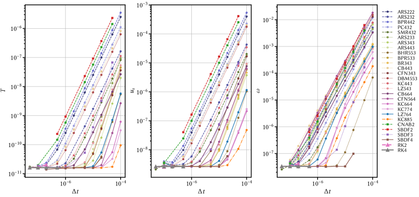
Figure 14: Convergence of the $\mathcal{L}^{2}$ error for the temperature field (left panel), the cylindrical radial velocity $u_{s}$ (middle panel) and the vorticity $\omega$ (right panel) for Case 3. In addition to the usual 26 IMEX schemes, this figure also features the fully explicit RK2 and RK4 methods, whose error levels are marked by large triangles which appear in the bottom left corner of each panel.

Appendix D Stability regions

In this section we give for completeness the stability regions of the explicit components of the 22 implicit explicit Runge–Kutta schemes, of the 4 IMEX multistep and of the two fully explicit schemes considered in this study. For an easier visual inspection of the stability domains, Fig. 15 has been split in three panels which gather the different expected orders of convergence of the combined IMEX schemes.

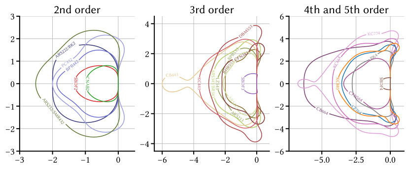
Figure 15: Stability regions of the explicit components of the 22 IMEX-RK, the 4 multistep and the 2 fully explicit schemes analyzed in this study. Schemes are stable inside the domains of the complex plane delimited by the curves. Left panel: order 2 schemes. Middle panel: order 3 schemes. Right panel: schemes of order 4 and 5. Order refers to the expected order of convergence of the combined IMEX schemes. Note that several schemes share the same stability domain for their explicit component: namely ARS222 and RK2; ARS232 and SMR432; ARS343, BR343 and RK4; AR233, BPR533 and LZ543.

Appendix E Error as a function of time to solution for cases 2 and 10

We provide in this appendix additional elements to assess the efficiency of the 26 schemes of interest in this study, providing metrics that may be more general than the dissipation-based efficiency introduced in Section 3.6. Figure 16 shows error against runtime for cases 2 and 10, whose convergence is analyzed in Section 3.2. This figure complements Figure 3 that displays error versus time step size $\Delta t$. Without getting into too much detail, we can stress that ARS343 appears as a good choice for case 2 and case 10. To obtain higher accuracy with a concomittent moderate increase in the computational cost, SBDF4 (for case 2) and KC664 (for case 10) should be preferred.

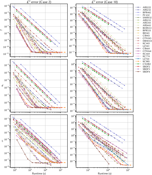
Figure 16: Convergence of the $\mathcal{L}^{2}$ error for the temperature field (top panels), the cylindrical radial velocity $u_{s}$ (middle panels) and the vorticity $\omega$ (bottom panels) for Case 2 (left column) and Case 10 (right column) as a function of total runtime expressed in seconds. The markers correspond to the class of IMEX, with squares denoting IMEX multistep and circles IMEX-RK multistage schemes. The total runtime is the product of the number of iterations times the average walltime, and ignores the initial computation and factorization of the requisite matrices.

Appendix F Expected behaviour of schemes for three dimensional simulations of planetary core dynamics

In this Appendix, we provide the reader with a conjectured efficiency that the considered time integrators could possibly have in 3-D spherical shell pseudo-spectral codes. In contrast with the current work where the linear solves are taking the largest amount of the walltimes, spherical harmonics transforms involved in the computation of the explicit terms are by a large margin the dominant player of spherical shell code algorithms. As such, under the asssumption that the CFL coefficients $\alpha^{\mbox{\scriptsize\sc max}}_{\mbox{\scriptsize\sc cfl}}$ are the same in 3-D, the conjectured efficiency of an individual time integrator for 3-D computations can be estimated using the number of explicit stages $n^{E}$

$$\mbox{eff}^{\text{3D}}=\frac{\alpha^{\mbox{\scriptsize\sc max}}_{\mbox{\scriptsize\sc cfl}}}{n^{E}}\,.$$ (23xev)

Figure 18 shows the conjectured efficiency in 3-D models relative to the efficiency of CNAB2. Compared to Fig. 13, all the schemes which necessitate an assembly stage have been penalized by the cost of the extra evaluation of an explicit state, with respect to the stiffly-accurate schemes. In contrast, the schemes with a lower number of explicit stages, such as BPR533, present an enhanced efficiency compared to the 2-D computations. PC432 stands out as the most efficient scheme for cases 2 and 5, while ARS343, BR343 and DBM553 become more efficient in the least stiff case 10. We anticipate that the overall gain in terms of efficiency compared to the CNAB2 method for 3-D calculations will be smaller than for our 2-D models, bounded to values between 20 and 30%.

Figure 18 shows the conjectured efficiency and accuracy in 3-D relative to CNAB2. This figure was obtained making the additional assumption that the 3-D computations would have similar errors than our 2-D computations. Focusing our attention on the upper right quadrant, one second order scheme (SMR432), three third order schemes (ARS343, BPR533 and CFN343) and one fourth order scheme (KC664) are always more efficient and more accurate than CNAB2 at the stability limit.

We stress that the reasoning put forward in this Appendix heavily relies on the assumptions that both the stability coefficients and the convergence curves are weakly affected by the change from 2-D to 3-D models. While this is a plausible hypothesis when considering the same physical phenomenon (i.e. non-rotating convection), the incorporation of additional physical effects such as rotation or a magnetic field is likely to significantly impact the convergence and the stability properties of the time integrators.

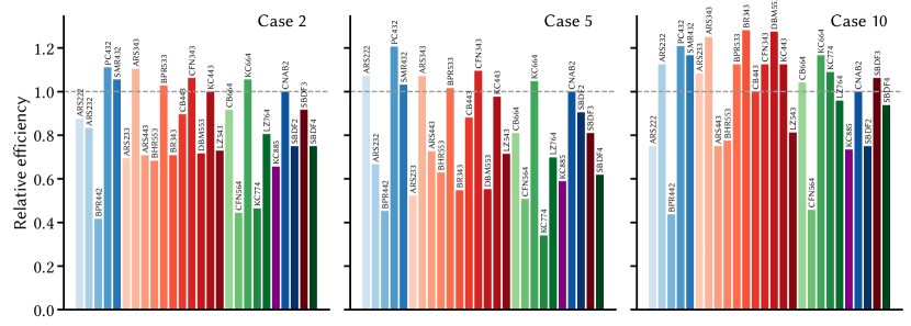
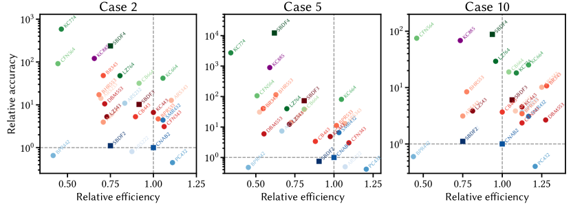
Figure 17: Conjectured efficiency in three-dimensions of the time integrators relative to the efficiency of CNAB2 for cases 2, 5 and 10 from left to right. Horizontal dashed lines correspond to a value of unity. See text for details.

Figure 18: Conjectured efficiency and accuracy in three-dimensions of the time integrators relative to the efficiency and accuracy of CNAB2 for cases 2, 5 and 10 from left to right. The scale on the $y$-axis is logarithmic. See text for details. Horizontal and vertical dashed lines correspond to a value of unity.

References

- McKenzie et al. (1974) D. P. McKenzie, J. M. Roberts, N. O. Weiss, Convection in the Earth’s mantle: towards a numerical simulation, Journal of Fluid Mechanics 62 (1974) 465–538.
- Sato and Thompson (1976) A. Sato, E. G. Thompson, Finite element models for creeping convection, Journal of Computational Physics 22 (1976) 229–244.
- Kopitzke (1979) U. Kopitzke, Finite element convection models: comparison of shallow and deep mantle convection, and temperatures in the mantle, Journal of Geophysics 46 (1979) 97–121.
- Jarvis (1984) G. T. Jarvis, Time-dependent convection in the Earth’s mantle, Physics of the Earth and Planetary Interiors 36 (1984) 305 – 327.
- Zhong et al. (2015) S. J. Zhong, D. A. Yuen, L. N. Moresi, M. G. Knepley, Numerical methods for mantle convection, in: G. Schubert (Ed.), Treatise on Geophysics, second edition ed., Elsevier, Oxford, 2015, pp. 197–222. URL: http://www.sciencedirect.com/science/article/pii/B9780444538024001305. doi:10.1016/B978-0-444-53802-4.00130-5.
- Davies et al. (2011) D. R. Davies, C. R. Wilson, S. C. Kramer, Fluidity: A fully unstructured anisotropic adaptive mesh computational modeling framework for geodynamics, Geochemistry, Geophysics, Geosystems 12 (2011) Q06001.
- Kronbichler et al. (2012) M. Kronbichler, T. Heister, W. Bangerth, High accuracy mantle convection simulation through modern numerical methods, Geophysical Journal International 191 (2012) 12–29.
- Canuto et al. (2006) C. Canuto, M. Y. Hussaini, A. Quarteroni, T. A. Zang, Spectral methods: Fundamentals in Single Domains, Scientific Computation, Springer, Berlin Heidelberg, 2006.
- Glatzmaier and Roberts (1995) G. A. Glatzmaier, P. H. Roberts, A three-dimensional convective dynamo solution with rotating and finitely conducting inner core and mantle, Physics of the Earth and Planetary Interiors 91 (1995) 63–75.
- Kageyama and Sato (1995) A. Kageyama, T. Sato, Computer simulation of a magnetohydrodynamic dynamo. II, Physics of Plasmas 2 (1995) 1421–1431.
- Glatzmaier (1984) G. A. Glatzmaier, Numerical simulations of stellar convective dynamos. I- The model and method, Journal of Computational Physics 55 (1984) 461–484.
- Clune et al. (1999) T. Clune, J. Elliott, M. Miesch, J. Toomre, G. Glatzmaier, Computational aspects of a code to study rotating turbulent convection in spherical shells, Parallel Computing 25 (1999) 361–380.
- Schaeffer (2013) N. Schaeffer, Efficient spherical harmonic transforms aimed at pseudospectral numerical simulations, Geochemistry, Geophysics, Geosystems 14 (2013) 751–758.
- Matsui et al. (2016) H. Matsui, E. Heien, J. Aubert, J. M. Aurnou, M. Avery, B. Brown, B. A. Buffett, F. Busse, U. R. Christensen, C. J. Davies, N. Featherstone, T. Gastine, G. A. Glatzmaier, D. Gubbins, J.-L. Guermond, Y.-Y. Hayashi, R. Hollerbach, L. J. Hwang, A. Jackson, C. A. Jones, W. Jiang, L. H. Kellogg, W. Kuang, M. Landeau, P. Marti, P. Olson, A. Ribeiro, Y. Sasaki, N. Schaeffer, R. D. Simitev, A. Sheyko, L. Silva, S. Stanley, F. Takahashi, S.-i. Takehiro, J. Wicht, A. P. Willis, Performance benchmarks for a next generation numerical dynamo model, Geochemistry, Geophysics, Geosystems 17 (2016) 1586–1607.
- Hollerbach (2000) R. Hollerbach, A spectral solution of the magneto-convection equations in spherical geometry, International Journal for Numerical Methods in Fluids 32 (2000) 773–797.
- Tilgner (1999) A. Tilgner, Spectral methods for the simulation of incompressible flows in spherical shells, International Journal for Numerical Methods in Fluids 30 (1999) 713–724.
- Ascher et al. (1997) U. M. Ascher, S. J. Ruuth, R. J. Spiteri, Implicit-explicit Runge–Kutta methods for time-dependent partial differential equations, Applied Numerical Mathematics 25 (1997) 151–167.
- Ascher et al. (1995) U. M. Ascher, S. J. Ruuth, B. T. R. Wetton, Implicit-explicit methods for time-dependent partial differential equations, SIAM Journal on Numerical Analysis 32 (1995) 797–823.
- Willis et al. (2007) A. P. Willis, B. Sreenivasan, D. Gubbins, Thermal core–mantle interaction: Exploring regimes for “locked” dynamo action, Physics of the Earth and Planetary Interiors 165 (2007) 83–92.
- Fournier et al. (2005) A. Fournier, H.-P. Bunge, R. Hollerbach, J.-P. Vilotte, A Fourier-spectral element algorithm for thermal convection in rotating axisymmetric containers, Journal of Computational Physics 204 (2005) 462–489.
- Stellmach and Hansen (2008) S. Stellmach, U. Hansen, An efficient spectral method for the simulation of dynamos in Cartesian geometry and its implementation on massively parallel computers, Geochemistry, Geophysics, Geosystems 9 (2008) Q05003.
- Verhoeven and Stellmach (2014) J. Verhoeven, S. Stellmach, The compressional beta effect: A source of zonal winds in planets?, Icarus 237 (2014) 143–158.
- Lecoanet et al. (2019) D. Lecoanet, G. M. Vasil, K. J. Burns, B. P. Brown, J. S. Oishi, Tensor calculus in spherical coordinates using Jacobi polynomials. part-II: Implementation and examples, Journal of Computational Physics: X 3 (2019) 100012.
- Marti et al. (2014) P. Marti, N. Schaeffer, R. Hollerbach, D. Cébron, C. Nore, F. Luddens, J. L. Guermond, J. Aubert, S. Takehiro, Y. Sasaki, Y. Y. Hayashi, R. Simitev, F. Busse, S. Vantieghem, A. Jackson, Full sphere hydrodynamic and dynamo benchmarks, Geophysical Journal International 197 (2014) 119–134.
- Livermore (2007) P. W. Livermore, An implementation of the exponential time differencing scheme to the magnetohydrodynamic equations in a spherical shell, Journal of Computational Physics 220 (2007) 824–838.
- Garcia et al. (2014) F. Garcia, L. Bonaventura, M. Net, J. Sánchez, Exponential versus IMEX high-order time integrators for thermal convection in rotating spherical shells, Journal of Computational Physics 264 (2014) 41–54.
- Garcia et al. (2010) F. Garcia, M. Net, B. García-Archilla, J. Sánchez, A comparison of high-order time integrators for thermal convection in rotating spherical shells, Journal of Computational Physics 129 (2010) 7997–8010.
- Glatzmaier and Roberts (1996) G. A. Glatzmaier, P. H. Roberts, An anelastic evolutionary geodynamo simulation driven by compositional and thermal convection, Physica D: Nonlinear Phenomena 97 (1996) 81–94.
- Spalart et al. (1991) P. R. Spalart, R. D. Moser, M. M. Rogers, Spectral methods for the Navier-Stokes equations with one infinite and two periodic directions, Journal of Computational Physics 96 (1991) 297–324.
- Yan et al. (2019) M. Yan, M. A. Calkins, S. Maffei, K. Julien, S. M. Tobias, P. Marti, Heat transfer and flow regimes in quasi-static magnetoconvection with a vertical magnetic field, Journal of Fluid Mechanics 877 (2019) 1186–1206.
- Marti et al. (2016) P. Marti, M. A. Calkins, K. Julien, A computationally efficient spectral method for modeling core dynamics, Geochemistry, Geophysics, Geosystems 17 (2016) 3031–3053.
- Cavaglieri and Bewley (2015) D. Cavaglieri, T. Bewley, Low-storage implicit/explicit Runge-Kutta schemes for the simulation of stiff high-dimensional ODE systems, Journal of Computational Physics 286 (2015) 172–193.
- Gastine (2019) T. Gastine, pizza: an open-source pseudo-spectral code for spherical quasi-geostrophic convection, Geophysical Journal International 217 (2019) 1558–1576.
- Boscarino et al. (2013) S. Boscarino, L. Pareschi, G. Russo, Implicit-explicit Runge–Kutta schemes for hyperbolic systems and kinetic equations in the diffusion limit, SIAM Journal on Scientific Computing 35 (2013) A22–A51.
- Tassin et al. (2021) T. Tassin, T. Gastine, A. Fournier, Geomagnetic semblance and dipolar-multipolar transition in top-heavy double-diffusive geodynamo models, Geophysical Journal International 226 (2021) 1897–1919.
- Grooms and Julien (2011) I. Grooms, K. Julien, Linearly implicit methods for nonlinear PDEs with linear dispersion and dissipation, Journal of Computational Physics 230 (2011) 3630–3650.
- Boscarino and Russo (2009) S. Boscarino, G. Russo, On a class of uniformly accurate IMEX Runge–Kutta schemes and applications to hyperbolic systems with relaxation, SIAM Journal on Scientific Computing 31 (2009) 1926–1945.
- Vos et al. (2011) P. E. Vos, C. Eskilsson, A. Bolis, S. Chun, R. M. Kirby, S. J. Sherwin, A generic framework for time-stepping partial differential equations (PDEs): general linear methods, object-oriented implementation and application to fluid problems, International Journal of Computational Fluid Dynamics 25 (2011) 107–125.
- Giraldo et al. (2013) F. X. Giraldo, J. F. Kelly, E. M. Constantinescu, Implicit-explicit formulations of a three-dimensional nonhydrostatic unified model of the atmosphere (NUMA), SIAM Journal on Scientific Computing 35 (2013) B1162–B1194.
- Gardner et al. (2018) D. J. Gardner, J. E. Guerra, F. P. Hamon, D. R. Reynolds, P. A. Ullrich, C. S. Woodward, Implicit–explicit (IMEX) Runge–Kutta methods for non-hydrostatic atmospheric models, Geoscientific Model Development 11 (2018) 1497–1515.
- Vogl et al. (2019) C. J. Vogl, A. Steyer, D. R. Reynolds, P. A. Ullrich, C. S. Woodward, Evaluation of implicit-explicit additive Runge-Kutta integrators for the HOMME-NH dynamical core, Journal of Advances in Modeling Earth Systems 11 (2019) 4228–4244.
- Ullrich et al. (2012) P. A. Ullrich, C. Jablonowski, J. Kent, P. H. Lauritzen, R. D. Nair, M. A. Taylor, Dynamical core model intercomparison project (DCMIP) test case document, DCMIP Summer School 83 (2012).
- Glatzmaier (2013) G. A. Glatzmaier, Introduction to Modeling Convection in Planets and Stars: Magnetic Field, Density Stratification, Rotation, Princeton University Press, 2013.
- Peyret (2002) R. Peyret, Spectral Methods for Incompressible Viscous Flow, Springer New York, 2002. URL: http://dx.doi.org/10.1007/978-1-4757-6557-1. doi:10.1007/978-1-4757-6557-1.
- Plaut and Busse (2002) E. Plaut, F. H. Busse, Low-Prandtl-number convection in a rotating cylindrical annulus, Journal of Fluid Mechanics 464 (2002) 345–363.
- King et al. (2012) E. M. King, S. Stellmach, J. M. Aurnou, Heat transfer by rapidly rotating Rayleigh–Bénard convection, Journal of Fluid Mechanics 691 (2012) 568–582.
- Press et al. (2007) W. H. Press, S. A. Teukolsky, W. T. Vetterling, B. P. Flannery, Numerical recipes: The art of scientific computing, 3 ed., Cambridge university press, 2007.
- Ascher and Petzold (1998) U. M. Ascher, L. R. Petzold, Computer Methods for Ordinary Differential Equations and Differential-Algebraic Equations, 1st ed., Society for Industrial and Applied Mathematics, USA, 1998.
- Hairer et al. (1993) E. Hairer, S. P. Nørsett, G. Wanner, Solving Ordinary Differential Equations I, volume 8 of Springer Series in Computational Mathematics, 2 ed., Springer-Verlag Berlin Heidelberg, 1993. doi:10.1007/978-3-540-78862-1.
- Hairer and Wanner (1996) E. Hairer, G. Wanner, Solving Ordinary Differential Equations II, volume 14 of Springer Series in Computational Mathematics, 2 ed., Springer-Verlag Berlin Heidelberg, 1996. doi:10.1007/978-3-642-05221-7.
- Kennedy and Carpenter (2003) C. A. Kennedy, M. H. Carpenter, Additive Runge–Kutta schemes for convection–diffusion–reaction equations, Applied Numerical Mathematics 44 (2003) 139–181.
- Julien and Watson (2009) K. Julien, M. Watson, Efficient multi-dimensional solution of PDEs using Chebyshev spectral methods, Journal of Computational Physics 228 (2009) 1480–1503.
- Boscarino (2007) S. Boscarino, Error analysis of imex runge–kutta methods derived from differential-algebraic systems, SIAM Journal on Numerical Analysis 45 (2007) 1600–1621.
- Pareschi and Russo (2005) L. Pareschi, G. Russo, Implicit–explicit runge–kutta schemes and applications to hyperbolic systems with relaxation, Journal of Scientific Computing 25 (2005) 129–155.
- Jameson et al. (1981) A. Jameson, W. Schmidt, E. Turkel, Numerical solution of the Euler equations by finite volume methods using Runge Kutta time stepping schemes, 1981. URL: https://arc.aiaa.org/doi/abs/10.2514/6.1981-1259. doi:10.2514/6.1981-1259. arXiv:https://arc.aiaa.org/doi/pdf/10.2514/6.1981-1259.
- Boscarino et al. (2017) S. Boscarino, L. Pareschi, G. Russo, A unified IMEX Runge--Kutta approach for hyperbolic systems with multiscale relaxation, SIAM Journal on Numerical Analysis 55 (2017) 2085--2109.
- Boscarino and Russo (2007) S. Boscarino, G. Russo, On the uniform accuracy of IMEX Runge-Kutta schemes and applications to hyperbolic systems with relaxation, in: Proceedings of SIMAI2006 VIII Convegno SIMAI Ragusa (Italy), May 2006, Communications to SIMAI Conferences, Society for Industrial and Applied Mathematics, Philadelphia, PA, 2007. doi:10.1685/CSC06028.
- Calvo et al. (2001) M. P. Calvo, J. de Frutos, J. Novo, Linearly implicit Runge--Kutta methods for advection--reaction--diffusion equations, Applied Numerical Mathematics 37 (2001) 535--549.
- Kinnmark and Gray (1984) I. P. Kinnmark, W. G. Gray, One step integration methods of third-fourth order accuracy with large hyperbolic stability limits, Mathematics and Computers in Simulation 26 (1984) 181–188.
- Liu and Zou (2006) H. Liu, J. Zou, Some new additive Runge–Kutta methods and their applications, Journal of Computational and Applied Mathematics 190 (2006) 74 -- 98. Special Issue: International Conference on Mathematics and its Application.
- Kennedy and Carpenter (2019) C. A. Kennedy, M. H. Carpenter, Higher-order additive Runge--Kutta schemes for ordinary differential equations, Applied Numerical Mathematics 136 (2019) 183--205.
- Johnston and Doering (2009) H. Johnston, C. R. Doering, Comparison of turbulent thermal convection between conditions of constant temperature and constant flux, Physical review letters 102 (2009) 064501.
- Frigo and Johnson (2005) M. Frigo, S. G. Johnson, The design and implementation of fftw3, Proceedings of the IEEE 93 (2005) 216--231.
- Anderson et al. (1999) E. Anderson, Z. Bai, C. Bischof, S. Blackford, J. D. J. Dongarra, J. D. Croz, A. Greenbaum, S. Hammarling, A. McKenney, D. Sorensen, LAPACK Users’ Guide, third ed., SIAM, Philadelphia, Pennsylvania, USA, 1999.
- Alonso et al. (2000) A. Alonso, J. Sánchez, M. Net, Transition to temporal chaos in an -symmetric convective system for low Prandtl numbers, Progress of Theoretical Physics Supplement 139 (2000) 315--324.
- Karniadakis et al. (1991) G. E. Karniadakis, M. Israeli, S. A. Orszag, High-order splitting methods for the incompressible Navier-Stokes equations, Journal of Computational Physics 97 (1991) 414–443.
- Gaspari and Cohn (1999) G. Gaspari, S. E. Cohn, Construction of correlation functions in two and three dimensions, Quarterly Journal of the Royal Meteorological Society 125 (1999) 723--757.
- Canuto et al. (2007) C. Canuto, M. Y. Hussaini, A. Quarteroni, T. A. Zang, Spectral methods: Evolution to Complex Geometries and Applications to Fluid Dynamics, Scientific Computation, Springer, Berlin Heidelberg, 2007.
- Virtanen et al. (2020) P. Virtanen, R. Gommers, T. E. Oliphant, M. Haberland, T. Reddy, D. Cournapeau, E. Burovski, P. Peterson, W. Weckesser, J. Bright, et al., SciPy 1.0: fundamental algorithms for scientific computing in python, Nature methods 17 (2020) 261--272.
- Hernandez et al. (2005) V. Hernandez, J. E. Roman, V. Vidal, SLEPc: A scalable and flexible toolkit for the solution of eigenvalue problems, ACM Trans. Math. Softw. 31 (2005) 351–362.
- Dalcin et al. (2011) L. D. Dalcin, R. R. Paz, P. A. Kler, A. Cosimo, Parallel distributed computing using Python, Advances in Water Resources 34 (2011) 1124--1139. New Computational Methods and Software Tools.
- Izzo and Jackiewicz (2017) G. Izzo, Z. Jackiewicz, Highly stable implicit–explicit Runge–Kutta methods, Applied Numerical Mathematics 113 (2017) 71–92.
- Kosloff and Tal-Ezer (1993) D. Kosloff, H. Tal-Ezer, A modified Chebyshev pseudospectral method with an time step restriction, Journal of Computational Physics 104 (1993) 457–469.
- Schwaiger et al. (2019) T. Schwaiger, T. Gastine, J. Aubert, Force balance in numerical geodynamo simulations: a systematic study, Geophysical Journal International 219 (2019) S101--S114.
- Gastine et al. (2020) T. Gastine, J. Aubert, A. Fournier, Dynamo-based limit to the extent of a stable layer atop Earth’s core, Geophysical Journal International 222 (2020) 1433--1448.
- Schaeffer et al. (2017) N. Schaeffer, D. Jault, H.-C. Nataf, A. Fournier, Turbulent geodynamo simulations: a leap towards Earth’s core, Geophysical Journal International 211 (2017) 1--29.
- Sheyko et al. (2018) A. Sheyko, C. Finlay, J. Favre, A. Jackson, Scale separated low viscosity dynamos and dissipation within the Earth’s core, Scientific Reports 8 (2018).
- Aubert (2019) J. Aubert, Approaching Earth’s core conditions in high-resolution geodynamo simulations, Geophysical Journal International 219 (2019) S137–S151.
- Zhang et al. (2016) H. Zhang, A. Sandu, S. Blaise, High order implicit-explicit general linear methods with optimized stability regions, SIAM Journal on Scientific Computing 38 (2016) 1430--1453.
- Giraldo and Restelli (2008) F. X. Giraldo, M. Restelli, A study of spectral element and discontinuous Galerkin methods for the Navier–Stokes equations in nonhydrostatic mesoscale atmospheric modeling: Equation sets and test cases, Journal of Computational Physics 227 (2008) 3849–3877.
- Wang and Ruuth (2008) D. Wang, S. J. Ruuth, Variable step-size implicit-explicit linear multistep methods for time-dependent partial differential equations, Journal of Computational Mathematics 26 (2008) 838--855.