Stable approximation of Helmholtz solutions in the disk
by evanescent plane waves

Abstract

Superpositions of plane waves are known to approximate well the solutions of the Helmholtz equation. Their use in discretizations is typical of Trefftz methods for Helmholtz problems, aiming to achieve high accuracy with a small number of degrees of freedom. However, Trefftz methods lead to ill-conditioned linear systems, and it is often impossible to obtain the desired accuracy in floating-point arithmetic. In this paper we show that a judicious choice of plane waves can ensure high-accuracy solutions in a numerically stable way, in spite of having to solve such ill-conditioned systems.

Numerical accuracy of plane wave methods is linked not only to the approximation space, but also to the size of the coefficients in the plane wave expansion. We show that the use of plane waves can lead to exponentially large coefficients, regardless of the orientations and the number of plane waves, and this causes numerical instability. We prove that all Helmholtz fields are continuous superposition of evanescent plane waves, i.e., plane waves with complex propagation vectors associated with exponential decay, and show that this leads to bounded representations. We provide a constructive scheme to select a set of real and complex-valued propagation vectors numerically. This results in an explicit selection of plane waves and an associated Trefftz method that achieves accuracy and stability.

The theoretical analysis is provided for a two-dimensional domain with circular shape. However, the principles are general and we conclude the paper with a numerical experiment demonstrating practical applicability also for polygonal domains.

Keywords: Helmholtz equation, Plane waves, Evanescent waves, Trefftz method, Stable approximation, Sampling, Frames, Reproducing kernel Hilbert spaces, Herglotz representation

AMS subject classification: 35J05, 41A30, 42C15, 44A15.

1 Introduction

The space dependence of time-harmonic solutions $U(\mathbf{x},t)=\Re\{e^{-\imath\omega t}u(\mathbf{x})\}$ of the scalar wave equation $\frac{1}{c^{2}}\frac{\partial^{2}U}{\partial t^{2}}-\Delta U=0$ is characterized by the homogeneous Helmholtz equation

$$-\Delta u-\kappa^{2}u=0.$$ (1.1)

The wavenumber is $\kappa:=\omega/c>0$, with $c$ the wave speed and $\omega$ the time frequency. Solutions of boundary value problems for the Helmholtz equation are oscillatory, making their numerical approximation notoriously computationally expensive at high frequencies, namely when the wavelength $\lambda:=2\pi/\kappa$ is much smaller than the characteristic length of the domain.

A well-studied way to efficiently represent Helmholtz solutions in a domain of $\mathbb{R}^{n}$ is to approximate them with linear combinations of propagative plane waves $\mathbf{x}\mapsto e^{\imath\kappa\mathbf{d}\cdot\mathbf{x}}$, which are particular solutions of (1.1) if the propagation direction $\mathbf{d}\in\mathbb{R}^{n}$ satisfies $\mathbf{d}\cdot\mathbf{d}=1$. Plane waves indeed offer better accuracy for fewer degrees of freedom compared to polynomial spaces, as supported by the theory developed in [30], building on previous results in [28, Sec. 8.4] and [9, Sec. 3.3.5]. Approximation by plane waves has been extensively used in the context of Trefftz schemes for the Helmholtz equation, a class of methods that use trial and test functions satisfying (1.1) locally on each element of a mesh, see [22] for a comprehensive survey. The simple expression of plane waves allows for very cheap implementations; for instance, integrals of products of these functions can be computed in closed form with wavenumber-independent effort, see [22, Sec. 4.1]. A second widespread use of plane wave approximation is the reconstruction of sound fields from point measurements (representing microphones) in experimental acoustics, see [11, 25, 34, 20].

The computation of plane wave approximations is however known to be numerically unstable, imposing strong limits to the achievable accuracy [33, 6]. This issue is often understood as an effect of the ill-conditioning of the linear system that is solved [22, Sec. 4.3], which inevitably arises from the almost-linear dependence of plane waves with similar propagation directions. Different techniques have been proposed to overcome this instability, e.g. [3, 15, 6]. A well-known recommendation suggests using not more than a prescribed number of waves in elements of a given size, e.g. [23, Eq. (14)]: this keeps the instability at bay but limits the achievable accuracy.

The first purpose of this paper is to shed a new light on the numerical instability experienced with propagative plane waves and explain the fundamental mathematical reasons for their limitations as described above. The second objective is to propose a practical remedy, in the form of including evanescent plane waves, which may decay exponentially in one direction, and using which one can achieve arbitrary accuracy in a numerically stable way. The approach is substantiated by theoretical analysis in combination with numerical evidence. As a first step in this direction, we focus mainly on the model approximation problem of Helmholtz solutions in the unit disk, using the modal analysis tools described in Section 2.

A new point of view on plane wave instability.

Recent advances in approximation theory, in particular based on the theory of frames and overcomplete bases [12], have shown that in the presence of ill-conditioning it is not sufficient to study best approximation errors in order to obtain accurate results in floating-point arithmetic [1, 2]. Rather, one is led to study the approximation error in relation to the coefficient norm, i.e., the norm of the coefficients in the expansion. The former depends solely on the approximation space, but the coefficient norm also depends on its chosen representation (i.e. on the spanning set used). We formalize this in Section 3 with the notion of stable approximation in Definition 3.1. The corresponding error analysis in Section 3.4, based largely on results in [1, 2], allows us to conclude in Section 4 that the set of propagative plane waves does not yield stable approximations. That is, we can formally state that there exist Helmholtz solutions, with relatively high Fourier frequency components in the angular coordinate, that are well approximated in the approximation space, but are nevertheless not numerically computable, see Theorem 4.3. In the terminology of approximation theory, no countable set of propagative plane waves is a frame for the space of Helmholtz solutions. (We recall that a frame of a Hilbert space is a natural generalization of a basis that allows for redundancy, see [12, 1].) In particular, it lacks a so-called lower frame bound which is the property that ensures that bounded functions can be represented with bounded coefficients. This point of view is reminiscent of a similar work in the context of the Method of Fundamental Solutions [5], which pre-dates the stability analysis from frame theory.

Unfortunately, while the theory in [1, 2] allows to identify this problem, it offers no concrete suggestions as to how it can be remedied. If the approximation space remains unchanged, a lower frame bound can only be established through a change of basis, such as orthogonalization as in [3, 15, 8]. However, that changes the representation: the solution would no longer be represented in the simple form of an expansion in plane waves, which is a key feature we would like to retain. Moreover, it may not be straightforward to ensure that the orthogonalization process itself is numerically stable.

The evanescent plane wave remedy.

To obtain stable representations, we propose to enrich the approximation space with evanescent plane waves, i.e. plane waves whose direction vectors are complex-valued, $\mathbf{d}\in\mathbb{C}^{n}$, as defined in Section 5. The Helmholtz equation is still satisfied provided $\mathbf{d}\cdot\mathbf{d}=1$ and, importantly, the expression remains simple and cheap to use in numerical schemes. Since their modulus decays exponentially in the direction $\Im[\mathbf{d}]$, evanescent plane waves are localized in bounded physical domains but also in the Fourier domain, hence are natural candidates for the approximation of the high frequency Fourier content exhibited by certain Helmholtz solutions. This idea is already present in the Wave Based Method, a special class of Trefftz schemes, see e.g. [17] for a survey. Evanescent plane waves also proved particularly effective in the approximation of interface problems in Trefftz methods, e.g. [27], and the approximation of integral kernels in some versions of the Fast Multipole Method [10].

To support the use of evanescent plane wave, we prove in Section 6 our main positive result, Theorem 6.7, which states that any Helmholtz solution in the unit disk can be uniquely represented in the form of a continuous superposition of evanescent plane waves. This integral representation has the key property of being stable, i.e. it features a provably bounded density (in a weighted $L^{2}$ space), and it can be seen as a generalization of the classical Herglotz representation, see e.g. [14, 35]. This result implies that evanescent plane waves form a continuous frame for the space of Helmholtz solutions, see Theorem 6.10. While this is stated at the continuous level, such a property paves the way for successful stable discrete expansions. Indeed, from the stability of the representation one may expect that discretizations exist with bounded coefficient norms, thereby solving the main issue with propagative plane waves.

A practical numerical recipe.

In view of practical implementations, we investigate the non-trivial task of identifying suitable sets of evanescent plane waves which deliver controllable accuracy in combination with stability. A heuristic choice for a set of complex directions $\mathbf{d}$ is suggested in [17, Sec. 3.2] (see also [22, Sec. 3.2]), but no mathematical justification is provided.

A first idea to obtain stable discrete representations (i.e. with bounded coefficients) would be to discretize the continous frame, but unfortunately, our setting does not fall within the assumptions of existing results (e.g. the boundedness assumption of [18, Th. 1.3] is not satisfied). Instead, the construction of approximation sets described in Section 7 is largely based on the optimal sampling procedure for weighted least-squares recently described by Cohen and Migliorati [13] (see also [21]) and subsequently used in [29], and it is illustrated with numerical experiments in Section 8. The strategy employed can be interpreted as the construction of a quadrature rule in the two-dimensional unbounded parametric domain of the integral representation. In practice, the recipe consists in drawing the quadrature points (i.e. select the directions of the plane waves) according to an explicit probability density function (7.7) which is a generalization to the multivariate setting of the Christoffel function density, The latter is sometimes called spectral function. While the rigorous numerical analysis of the above approach is thus far incomplete, we conjecture that such a construction provides stable discrete representations, see Conjecture 7.1. In fact, the experimental results in Section 8 show that the resulting approximations are both controllably accurate and numerically stable, provided one uses sufficient oversampling and regularization.

Although the recipe is derived from the analysis on the disk, we include numerical results on a triangular cell showing that it appears to be effective also for other shapes. Approximation and stability properties of evanescent plane waves in more general domains and their use in mesh-based Trefftz methods (e.g. the Trefftz-Discontinuous Galerkin method [22, Sec. 2.2]) will be considered in future publications (see [19] for the extension of the theory of this paper to three-dimensional problems).

2 Helmholtz equation in circular geometry

We first present the setting of the paper and introduce notation. The proofs of the statements follow standard arguments and are collected in Appendix A.

2.1 Circular waves

In this paper we only consider circular two-dimensional geometries. Without loss of generality, we assume that the domain is the open unit disk, henceforth denoted $B_{1}:=\{\mathbf{x}\in\mathbb{R}^{2}|\;\|\mathbf{x}\|<1\}$. The circular geometry enables modal analysis via separation of variables. The circular waves are the bounded solutions of the Helmholtz equation in the unit disk that are separable in polar coordinates. They are sometimes also referred to as Fourier–Bessel functions or as Generalized Harmonic Polynomials [28].

The results of this paper are fomulated most concisely using the following $\kappa$-dependent scalar product and norm: for any $u,v\in H^{1}(B_{1})$,

$$\left(u,\,v\right)_{\mathcal{B}}:=\left(u,\,v\right)_{L^{2}(B_{1})}+\kappa^{-2}\left(\nabla u,\,\nabla v\right)_{L^{2}(B_{1})},\qquad\qquad\|u\|_{\mathcal{B}}^{2}:=\left(u,\,u\right)_{\mathcal{B}}.$$ (2.1)

Definition 2.1 (Circular waves).

We define, for any $p\in\mathbb{Z}$

$$\begin{cases}\tilde{b}_{p}(\mathbf{x}):=J_{p}(\kappa r)e^{\imath p\theta},\quad\forall\mathbf{x}=\left(r,\,\theta\right)\in B_{1},\\ b_{p}:=\beta_{p}\tilde{b}_{p},\quad\text{where}\quad\beta_{p}:=\|\tilde{b}_{p}\|_{\mathcal{B}}^{-1},\end{cases}\quad\text{and}\qquad\mathcal{B}:=\overline{\operatorname{span}\left\{{b}_{p}\right\}_{p\in\mathbb{Z}}}^{\|\cdot\|_{\mathcal{B}}}\subsetneq H^{1}(B_{1}).$$ (2.2)

In this definition, $J_{p}$ is the usual Bessel function of the first kind [31, Eq. (10.2.2)] and $\imath$ the imaginary unit $\imath^{2}=-1$. The space $\mathcal{B}$ is a strict subspace of $H^{1}(B_{1})$, whose elements are solutions of the Helmholtz equation, see Lemma 2.3 below. A representation of the real part of some circular waves is given in Figure 1. We will refer to the circular waves with mode number $|p|<\kappa$ as propagative modes. The ‘energy’ of such modes is distributed in the bulk of the domain. On the contrary, for $|p|\gg\kappa$, the circular waves are termed evanescent. Their ‘energy’ is concentrated near the boundary of the domain. In between, the waves such that $|p|\approx\kappa$ are called grazing modes.

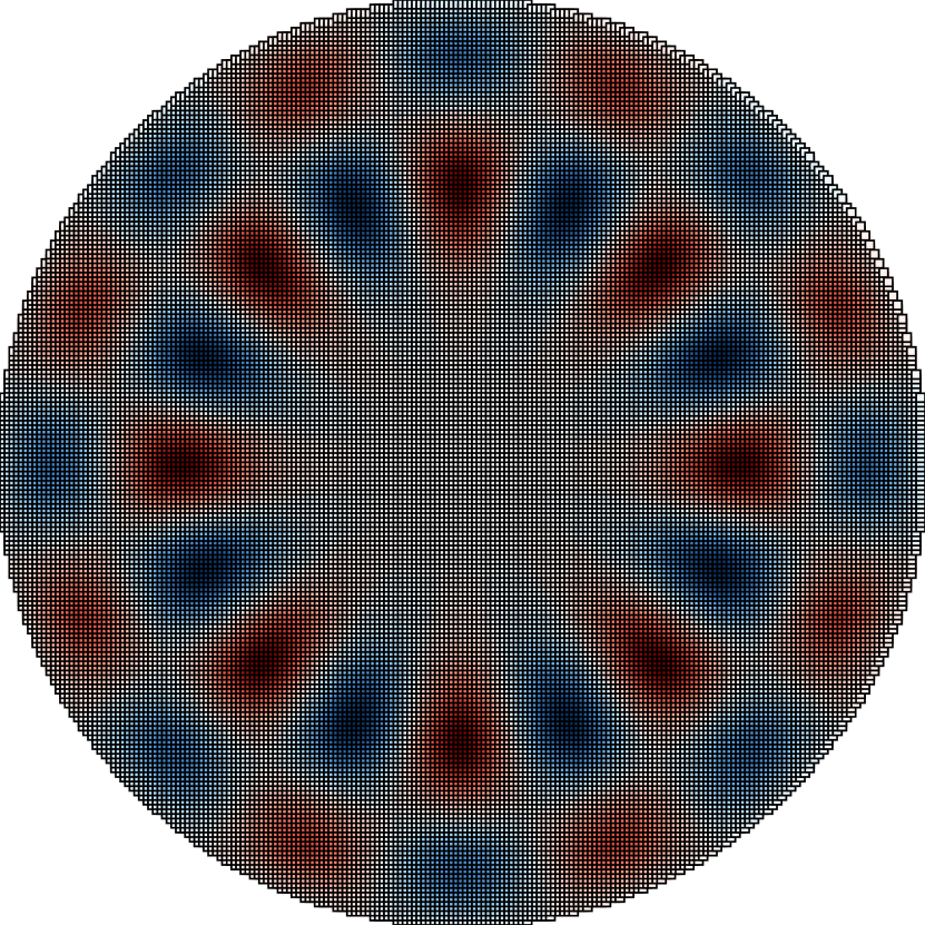
(a) Propagative $p=8$.

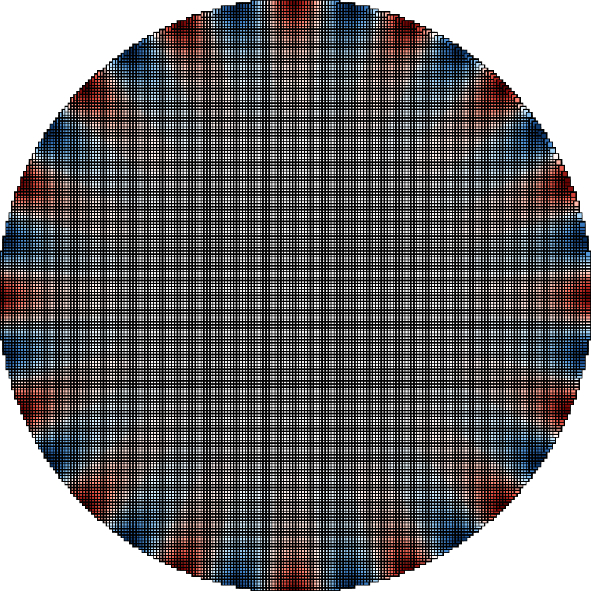
(b) Grazing $p=16$.

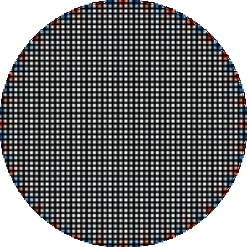
(c) Evanescent $p=32$.

Figure 1: Real part of the circular waves $\tilde{b}_{p}$ for three different modes (wavenumber $\kappa=16$).

Lemma 2.2.

The space $\left(\mathcal{B},\,\|\cdot\|_{\mathcal{B}}\right)$ is a Hilbert space and the family $\{b_{p}\}_{p\in\mathbb{Z}}$ is a Hilbert basis (i.e. an orthonormal basis):

$$\left(b_{p},\,b_{q}\right)_{\mathcal{B}}=\delta_{pq},\qquad\forall p,q\in\mathbb{Z},\qquad\text{and}\qquad u=\sum_{p\in\mathbb{Z}}\left(u,\,b_{p}\right)_{\mathcal{B}}b_{p},\qquad\forall u\in\mathcal{B}.$$ (2.3)

The main reason for introducing circular waves is the possibility to use them to expand any Helmholtz solution on the disk, as we show in the next lemma. Related results for more general domains and different norms are available, see e.g. [22, Sec. 3.1].

Lemma 2.3.

$u\in H^{1}(B_{1})$ satisfies the Helmholtz equation (1.1) if and only if $u\in\mathcal{B}$.

Circular and spherical waves have been used as basis functions in many Trefftz schemes, see [22, Sec. 3.1] and the references therein. An interesting feature of such waves is that the approximation sets are naturally hierarchical.

2.2 Asymptotics of normalization coefficients

The normalization coefficients $\beta_{p}$ in (2.2) grow super-exponentially with $|p|$ after a pre-asymptotic regime up to $|p|\approx\kappa$. The precise asymptotic behavior is given by the following lemma.

Lemma 2.4.

For all $p\in\mathbb{Z}$,

$$\beta_{p}=\left(2\pi\left[J_{p}^{2}(\kappa)-J_{p-1}(\kappa)J_{p+1}(\kappa)+J_{p}^{\prime}(\kappa)J_{p}(\kappa)/\kappa\right]\right)^{-1/2}\underset{|p|\to+\infty}{\sim}\kappa\left(\frac{2}{e\kappa}\right)^{|p|}\;|p|^{|p|}.$$ (2.4)

Remark 2.5.

The circular waves are normalized using the rather natural $\mathcal{B}$ norm (2.1), i.e. the wavenumber-weighted $H^{1}(B_{1})$ norm. The use of $L^{2}(B_{1})$ or other Sobolev norms in the definition of $\beta_{p}$ would not modify the exponential dependence on $|p|$ of the asymptotics (2.4), but it does introduce an additional moderate power of $|p|$, as is visible in the proof in Appendix A.

3 Stable numerical approximation

The purpose of this section is to explain the crucial notion of stable approximation, which we could informally call “approximation with small coefficients”, and to clarify how it enables accurate numerical computations. Our approach builds on the results in [1, 2] which highlight the importance for stability of having representations with bounded coefficients. We also describe the practical procedure, a regularized sampling method, that we use to investigate the existence of stable numerical approximations of Helmholtz solutions in this paper. An error bound is formulated in Proposition 3.2.

3.1 The notion of stable approximation

Let us consider a sequence of finite approximation sets in $\mathcal{B}$

$$\boldsymbol{\Phi}:=\{\boldsymbol{\Phi}_{k}\}_{k\in\mathbb{N}}\qquad\text{where}\qquad\boldsymbol{\Phi}_{k}:=\{\phi_{k,l}\}_{l},\quad|\boldsymbol{\Phi}_{k}|<\infty,\quad\forall k\in\mathbb{N},$$ (3.1)

and for each $k,l$, $\phi_{k,l}\in\mathcal{B}$ is a solution of the Helmholtz equation (1.1) in the unit disk. These sets need not be nested. When the $\{\phi_{k,l}\}_{l}$ are linearly independent, $\boldsymbol{\Phi}_{k}$ is a basis of the approximation space used for numerical computations. However, more generally, we also allow for linearly dependent sets. Associated to any set $\boldsymbol{\Phi}_{k}$ for some $k\in\mathbb{N}$, we define the synthesis operator

$$\mathcal{T}_{\boldsymbol{\Phi}_{k}}\;:\;\mathbb{C}^{|\boldsymbol{\Phi}_{k}|}\to\mathcal{B},\ \boldsymbol{\mu}=\{\mu_{l}\}_{l}\mapsto\sum_{l}\mu_{l}\phi_{k,l}.$$ (3.2)

Here and in the following, we use the notation $|X|$ to indicate the cardinality of the set $X$. We are now ready to define a notion of stable approximation, which is at the heart of this paper.

Definition 3.1 (Stable approximation).

The sequence $\boldsymbol{\Phi}$ of approximation sets (3.1) is said to be a stable approximation for $\mathcal{B}$ if, for any tolerance $\eta>0$, there exist a stability exponent $s\geq 0$ and a stability constant $C_{\mathrm{stb}}\geq 0$ such that

$$\forall u\in\mathcal{B},\ \exists\,\boldsymbol{\Phi}_{k}\in\boldsymbol{\Phi},\ \boldsymbol{\mu}\in\mathbb{C}^{|\boldsymbol{\Phi}_{k}|}\quad\text{such that}\quad\begin{cases}\|u-\mathcal{T}_{\boldsymbol{\Phi}_{k}}{\boldsymbol{\mu}}\|_{\mathcal{B}}\leq\eta\|u\|_{\mathcal{B}}\quad\text{and}\\[2.84526pt] \|\boldsymbol{\mu}\|_{\ell^{2}}\leq C_{\mathrm{stb}}|\boldsymbol{\Phi}_{k}|^{s}\|u\|_{\mathcal{B}}.\end{cases}$$ (3.3)

Having a sequence of stable approximation sets means that one can approximate any Helmholtz solution to a given accuracy in the form of a finite expansion $\mathcal{T}_{\boldsymbol{\Phi}_{k}}{\boldsymbol{\mu}}$ where the coefficients $\boldsymbol{\mu}$ have bounded $\ell^{2}$-norm. This bound on the coefficients admits a polynomial growth in the number $|\boldsymbol{\Phi}_{k}|$ of terms in the expansion, but not an exponential growth. The stability exponent $s\geq 0$ of a stable approximation sequence controls the growth of the coefficient norm $\|\mu\|_{\ell^{2}}$: the smaller $s$ the more stable the sequence. This notion of stability is not related to a space but rather to a particular sequence of sets that are used to represent the numerical approximation. In practice the computation of approximations using stable sequences may lead to ill-conditioned linear systems if there is redundancy in the approximation sets. The rest of this section shows that, in spite of possible ill-conditioning, stable sequences lead to accurate approximations, thanks to the boundedness of the expansion coefficients.

The simplest stable approximation is provided by the truncation of any orthonormal basis of $\mathcal{B}$, in which case $s=0$ and $C_{\mathrm{stb}}=1$, e.g. the circular waves $\boldsymbol{\Phi}_{k}=\{b_{p}\}_{|p|\leq k}$. However, in view of the application to Trefftz methods on polygonal meshes, we describe two examples of approximations sets of the type of (3.1): propagative plane waves (PPWs) in (4.2) and evanescent plane waves (EPWs) in (7.11). They exhibit different stability properties. In Theorem 4.3 we prove rigorously that PPWs are necessarily unstable. In contrast, numerical evidence from Section 8 indicates that the sets of EPWs constructed following the numerical recipe that we propose in Section 7.3 are stable.

3.2 Boundary sampling method

We explain how we compute the coefficients in practice, which builts on results in [24]. All the numerical results obtained in this paper are obtained using the method described here.

Let us introduce a ‘trace operator’ $\gamma$, namely a (continuous) linear operator defined on $H^{1}(B_{1})$ such that the following problem is well-posed: find $u\in H^{1}(B_{1})$ such that

$$-\Delta u-\kappa^{2}u=0,\quad\text{in}\ B_{1},\qquad\text{and}\qquad\gamma u=g,\quad\text{on}\ \partial B_{1},$$ (3.4)

for some suitable boundary data $g$. Examples of such a trace operator $\gamma$ are: the Dirichlet trace operator, extension to $H^{1}(B_{1})$ of $u\mapsto u|_{\partial B_{1}}$, when $\kappa^{2}$ is not an eigenvalue of the Dirichlet Laplacian; the Neumann trace operator, extension to $H^{1}(B_{1})$ of $u\mapsto\partial_{\mathbf{n}}u$, when $\kappa^{2}$ is not an eigenvalue of the Neumann Laplacian; the Robin trace operator, extension to $H^{1}(B_{1})$ of $u\mapsto\partial_{\mathbf{n}}u-\imath\kappa u|_{\partial B_{1}}$ (without assumptions on the wavenumber $\kappa$).

We aim at reconstructing a solution $u\in\mathcal{B}$ having access to its trace $\gamma u$ on the boundary for such a ‘good’ trace operator $\gamma$. For simplicity, we use the Dirichlet trace operator and therefore assume that $\kappa^{2}$ is away from the eigenvalues of the Dirichlet Laplacian. Further we will assume that $u\in\mathcal{B}\cap C^{0}(\overline{B_{1}})$, so that it makes sense to consider point evaluations of the Dirichlet trace.

The reconstruction process is not the main subject of the paper and we stress that we make these two assumptions mainly for convenience and definiteness (in particular for the numerical experiments). One can consider alternative reconstruction procedures using other types of data, such as point evaluation in the bulk of the domain or by taking inner product of the solution with suitable test functions. See [11] for a more general discussion on the subject of reconstructing Helmholtz solutions from point evaluations.

Let $u\in\mathcal{B}\cap C^{0}(\overline{B_{1}})$ be the target of the approximation problem. We look for a set of coefficients $\boldsymbol{\xi}\in\mathbb{C}^{|\boldsymbol{\Phi}_{k}|}$ for a given approximation set $\boldsymbol{\Phi}_{k}$ (introduced in (3.1)) such that $\mathcal{T}_{\boldsymbol{\Phi}_{k}}\boldsymbol{\xi}\approx u$. We also assume that for any $l$, $\phi_{k,l}\in\mathcal{B}\cap C^{0}(\overline{B_{1}})$. Define the set of $S\geq|\boldsymbol{\Phi}_{k}|$ sampling points $\{\mathbf{x}_{s}\}_{s=1}^{S}$ on the unit circle parametrized by the angle

$$\theta_{s}:=\frac{2\pi s}{S},\qquad 1\leq s\leq S.$$ (3.5)

Let us introduce the matrix $A=(A_{s,l})_{s,l}\in\mathbb{C}^{S\times|\boldsymbol{\Phi}_{k}|}$ and the vector $\mathbf{b}=(\mathbf{b}_{s})_{s}\in\mathbb{C}^{S}$ such that

$$A_{s,l}=\gamma(\phi_{k,l})(\mathbf{x}_{s}),\quad\mathbf{b}_{s}=(\gamma u)(\mathbf{x}_{s}),\qquad\qquad 1\leq l\leq|\boldsymbol{\Phi}_{k}|,\ 1\leq s\leq S.$$ (3.6)

The sampling method then consists in approximately solving the rectangular linear system

$$A\boldsymbol{\xi}=\mathbf{b}.$$ (3.7)

3.3 Regularization

It often happens that the matrix $A$ is ill-conditioned (see Section 4.3). In finite precision arithmetic, severe ill-conditioning may prevent us from obtaining accurate approximations. However, the type of ill-conditioning encountered here is benign if it arises only from the redundancy of the approximating functions. In that case, ill-conditioning is associated with the numerical non-uniqueness of the solution of the linear system, yet all associated expansions may approximate the target to similar accuracy. If among those expansions there exist some with small coefficient norms, then it is possible to numerically compute an accurate approximation. To this aim, we rely on the combination of oversampling and regularization techniques developed in [1, 2]. Alternative techniques to curb ill-conditioning can be found in the literature, see [3] where a suitable change of basis is used that works well for circular geometries, [15] which uses orthogonalization, and [6, 24] in the context of Trefftz methods.

The first step is to compute the Singular Value Decomposition (SVD) of the matrix $A$, namely

$$A=U\Sigma V^{*}.$$ (3.8)

Let us denote by $(\sigma_{m})_{m}$ for $m=1,\dots,|\boldsymbol{\Phi}_{k}|$ the singular values of $A$, assumed to be sorted in descending order. For notational clarity, the largest singular value is renamed $\sigma_{\max}:=\sigma_{1}$. Then, the regularization amounts to trimming the tail of relatively small singular values, which are approximated by zero. Let $\epsilon\in(0,1]$ be a chosen threshold, we denote by $\Sigma_{\epsilon}$ the approximation of the diagonal matrix $\Sigma$ where all diagonal elements $\sigma_{m}$ such that $\sigma_{m}<\epsilon\sigma_{\max}$ are replaced by zero. This leads to the approximate factorization

$$A_{S,\epsilon}:=U\Sigma_{\epsilon}V^{*},$$ (3.9)

of the matrix $A$. An approximate solution to (3.7) is then obtained by

$$\boldsymbol{\xi}_{S,\epsilon}:=A_{S,\epsilon}^{\dagger}\mathbf{b}=V\Sigma_{\epsilon}^{\dagger}U^{*}\,\mathbf{b}.$$ (3.10)

Here $\Sigma_{\epsilon}^{\dagger}$ denotes the pseudo-inverse of the matrix $\Sigma_{\epsilon}$, namely the diagonal matrix with $(\Sigma_{\epsilon}^{\dagger})_{j,j}=(\Sigma_{j,j})^{-1}$ if $\Sigma_{j,j}\geq\epsilon\sigma_{\max}$ and $(\Sigma_{\epsilon}^{\dagger})_{j,j}=0$ otherwise. Robust computation of $\boldsymbol{\xi}_{S,\epsilon}$ requires to compute the right-hand-side of (3.10) from right to left, namely $\boldsymbol{\xi}_{S,\epsilon}:=V\left(\Sigma_{\epsilon}^{\dagger}\left(U^{*}\,\mathbf{b}\right)\right)$, in order to avoid mixing small and large values on the diagonal of $\Sigma_{\epsilon}^{\dagger}$.

3.4 Error estimates for the sampling method with regularization

With the regularization technique described above together with oversampling, i.e., $S$ larger than $|\boldsymbol{\Phi}_{k}|$, accurate approximations can be effectively computed, provided the set sequence is a stable approximation in the sense of Definition 3.1. This broad statement is the main message of [1, Th. 5.3] and [2, Th. 1.3 and 3.7], and is the starting point of our quest of stable approximation sets for Helmholtz solutions. More precisely, the following proposition is a rewording of [2, Th. 3.7] from the context of generalized sampling to our setting, with the notations just introduced. See Appendix B for the proof.

Proposition 3.2.

Let $\gamma$ be the Dirichlet trace operator and $u\in\mathcal{B}\cap C^{0}(\overline{B_{1}})$. Given some approximation set $\boldsymbol{\Phi}_{k}$ ($k\in\mathbb{N}$ fixed) such that for any $l$, $\phi_{k,l}\in\mathcal{B}\cap C^{0}(\overline{B_{1}})$; a sampling set of size $S\in\mathbb{N}$ as described in (3.5) and some regularization parameter $\epsilon\in(0,1]$, we consider the approximate solution of the linear system (3.7), namely $\boldsymbol{\xi}_{S,\epsilon}\in\mathbb{C}^{|\boldsymbol{\Phi}_{k}|}$ as defined in (3.10). Then

$$\forall\boldsymbol{\mu}\in\mathbb{C}^{|\boldsymbol{\Phi}_{k}|},\,\exists S_{0}>0,\forall S\geq S_{0},$$ (3.11)

$$\|\gamma(u-\mathcal{T}_{\boldsymbol{\Phi}_{k}}\boldsymbol{\xi}_{S,\epsilon})\|_{L^{2}(\partial B_{1})}\leq 3\|\gamma(u-\mathcal{T}_{\boldsymbol{\Phi}_{k}}\boldsymbol{\mu})\|_{L^{2}(\partial B_{1})}+2\sqrt{\pi}\,\frac{\epsilon\,\sigma_{\max}}{\sqrt{S}}\|\boldsymbol{\mu}\|_{\ell^{2}}.$$

Assume moreover that $\kappa^{2}$ is not an eigenvalue of the Dirichlet Laplacian in $B_{1}$. Then, there exists a constant $C_{\mathrm{err}}$ independent of $u$ and $\boldsymbol{\Phi}_{k}$, such that

$$\forall\boldsymbol{\mu}\in\mathbb{C}^{|\boldsymbol{\Phi}_{k}|},\,\exists S_{0}>0,\ \forall S\geq S_{0},$$ (3.12)

$$\|u-\mathcal{T}_{\boldsymbol{\Phi}_{k}}\boldsymbol{\xi}_{S,\epsilon}\|_{L^{2}(B_{1})}\leq C_{\mathrm{err}}\Big{(}\|u-\mathcal{T}_{\boldsymbol{\Phi}_{k}}\boldsymbol{\mu}\|_{\mathcal{B}}+\frac{\epsilon\,\sigma_{\max}}{\sqrt{S}}\|\boldsymbol{\mu}\|_{\ell^{2}}\Big{)}.$$

Proposition 3.2 shows that having stable approximation sets in the sense of Definition 3.1 is a sufficient condition for the accurate reconstruction of a Helmholtz solution from its samples on the boundary of the disk, provided enough sampling points $S$ and a sufficiently small regularization parameter $\epsilon$ are used. This is summed up in the following result, see Appendix B for its proof.

Corollary 3.3.

Let $\delta>0$. We assume to have a sequence of approximation sets $\{\boldsymbol{\Phi}_{k}\}_{k\in\mathbb{N}}$ that is stable in the sense of Definition 3.1. Assume also that $\kappa^{2}$ is not a Dirichlet eigenvalue in $B_{1}$. Then,

$$\forall u\in\mathcal{B}\cap C^{0}(\overline{B_{1}}),\ \exists\boldsymbol{\Phi}_{k},\ S_{0}>0,\ \epsilon_{0}\in(0,1],\quad\text{such that}\quad$$ (3.13)

$$\forall S\geq S_{0},\epsilon\in(0,\epsilon_{0}],\qquad\|u-\mathcal{T}_{\boldsymbol{\Phi}_{k}}\boldsymbol{\xi}_{S,\epsilon}\|_{L^{2}(B_{1})}\leq\delta\|u\|_{\mathcal{B}},$$

where $\boldsymbol{\xi}_{S,\epsilon}\in\mathbb{C}^{|\boldsymbol{\Phi}_{k}|}$ is defined in (3.10). Moreover, we can take the regularization parameter $\epsilon$ as large as

$$\epsilon_{0}=\frac{\delta\;\sqrt{S}}{2C_{\mathrm{err}}\sigma_{\max}C_{\mathrm{stb}}|\boldsymbol{\Phi}_{k}|^{s}}.$$ (3.14)

The point of Corollary 3.3 is not only that the solution of the regularized SVD problem provides an accurate approximation of $u$, but also that it is numerically computable. This is in contrast with the classical theory for the approximation by PPWs, e.g. [30], which provides rigorous best-approximation error bounds that often can not be attained numerically, precisely because accurate approximations require large coefficients and cancellation, so exact-arithmetic results cannot be reflected by floating-point computations.

The assumption on the eigenvalues in Corollary 3.3 can be lifted if in (3.13) the $L^{2}(B_{1})$ norm is replaced by $L^{2}(\partial B_{1})$. Moreover, in this case, the constant $C_{\mathrm{err}}$ at the right-hand side of (3.14) can be dropped. Finally, the largest singular value $\sigma_{\max}$ of the matrix $A$ appears in the above results: in our numerical experiments $\sigma_{\max}$ is moderate, see Figure 10.

In the following, it will be convenient to measure the approximation error by the relative residual

$$\mathcal{E}=\mathcal{E}(u,\boldsymbol{\Phi}_{k},S,\epsilon):=\frac{\|A\boldsymbol{\xi}_{S,\epsilon}-\mathbf{b}\|_{\ell^{2}}}{\|\mathbf{b}\|_{\ell^{2}}},$$ (3.15)

where $\boldsymbol{\xi}_{S,\epsilon}$ is the solution (3.10) of the regularized linear system. Arguing as in the proof of Proposition 3.2, (see Appendix B) for sufficiently large $S$, the quantity $\mathcal{E}$ satisfies (for a constant $\tilde{C}$ independent of $u$, $\boldsymbol{\Phi}_{k}$, $S$)

$$\|u-\mathcal{T}_{\boldsymbol{\Phi}_{k}}\boldsymbol{\xi}_{S,\epsilon}\|_{L^{2}(B_{1})}\leq\tilde{C}\|u\|_{\mathcal{B}}\;\mathcal{E}.$$ (3.16)

4 Instability of propagative plane wave sets

The purpose of this section is to present the pitfalls encountered when using propagative plane waves (PPW) to approximate Helmholtz solutions in the unit disk. In particular, we show that PPWs with equispaced angles in general fail to yield stable approximations. This implies that problems can not be solved numerically to arbitrary accuracy or, in some cases, to any accuracy at all. The main effort is to show that PPW approximations lead to large expansion coefficients and that this problem can not be avoided using PPWs alone.

4.1 Propagative plane waves and Jacobi–Anger identity

We introduce the notion of a propagative plane wave. The adjective propagative is not customary in the literature, but serves to distinguish the following definition with the notion of evanescent plane waves (EPWs) that will be introduced in Definition 5.1.

Definition 4.1 (Propagative plane wave).

For any angle $\varphi\in[0,2\pi)$, we let

$$\mathrm{PW}_{\varphi}(\mathbf{x}):=e^{\imath\kappa\mathbf{d}(\varphi)\cdot\mathbf{x}},\ \forall\mathbf{x}\in\mathbb{R}^{2},\quad\text{where}\quad\mathbf{d}(\varphi):=\left(\cos\varphi,\,\sin\varphi\right)\in\mathbb{R}^{2}.$$ (4.1)

All PPWs satisfy the homogeneous Helmholtz equation (1.1) since $\mathbf{d}(\varphi)\cdot\mathbf{d}(\varphi)=1$ for any angle $\varphi\in[0,2\pi)$.

Propagative plane waves are a common choice in Trefftz schemes, see [22, Sec. 3.2] and the references therein. In 2D, isotropic approximations are obtained by using equispaced angles: for some $M\in\mathbb{N}$, the approximation set is defined as

$$\boldsymbol{\Phi}_{M}:=\{M^{-1/2}\,\mathrm{PW}_{\varphi_{M,m}}\}_{m=1}^{M},\quad\text{where}\quad\varphi_{M,m}:=\frac{2\pi m}{M},\qquad 1\leq m\leq M.$$ (4.2)

In contrast to circular waves, the approximation sets based on such PPWs are in general not hierarchical. Plane waves spaces have been studied in the literature, in particular explicit $hp$-estimates in suitable Sobolev semi-norms are available for general domains, see [30, Th. 5.2 and 5.3]. These results ensure more than exponential convergence (with respect to the number of plane waves used) of the approximation of homogeneous Helmholtz solutions by a finite superposition of PPWs. Therefore, at least in principle, PPWs are well-suited for Trefftz approximations.

The Jacobi–Anger identity [31, Eq. (10.12.1)] provides a link between plane waves and circular waves and is ubiquitous in the analysis that follows:

$$\mathrm{PW}_{\varphi}(r,\theta)=e^{\imath\kappa\mathbf{d}(\varphi)\cdot\mathbf{x}}=\sum_{p\in\mathbb{Z}}\imath^{p}J_{p}(\kappa r)e^{\imath p(\theta-\varphi)},\qquad\forall\mathbf{x}=(r,\theta)\in B_{1},\ \varphi\in[0,2\pi).$$ (4.3)

4.2 Herglotz representation

We recall the so-called Herglotz functions. They are defined for any $v\in L^{2}([0,2\pi])$ as

$$u(\mathbf{x};v):=\int_{0}^{2\pi}v(\varphi)\mathrm{PW}_{\varphi}(\mathbf{x})\;\mathrm{d}\varphi,\qquad\forall\mathbf{x}\in\mathbb{R}^{2},$$ (4.4)

see [14, Eq. (1.1)], [35, Eq. (6)] and [16, Def. 3.18]. Such an expression is termed Herglotz representation. The function $v$ is called Herglotz kernel or density. These functions $u(\cdot;v)\in C^{\infty}(\mathbb{R}^{2})$ are entire solutions of the Helmholtz equation and can be seen as a continuous superposition of PPWs, weighted according to $v$. To see that $u(\cdot,v)\in\mathcal{B}$, let $v\in L^{2}([0,2\pi])$, which we write as a Fourier expansion

$$v(\varphi)=\frac{1}{2\pi}\sum_{p\in\mathbb{Z}}\hat{v}_{p}e^{\imath p\varphi},\qquad\forall\varphi\in[0,2\pi],$$ (4.5)

for a sequence of coefficients $(\hat{v}_{p})_{p\in\mathbb{Z}}\in\ell^{2}(\mathbb{Z})$. Plugging this expression into (4.4) and using the Jacobi–Anger expansion (4.3) together with the orthogonality of the complex exponentials $\{\theta\mapsto e^{\imath p\theta}\}_{p\in\mathbb{Z}}$, we obtain, for any $\mathbf{x}=(r,\theta)\in\mathbb{R}^{2}$,

$$u(\mathbf{x};v)=\int_{0}^{2\pi}v(\varphi)\mathrm{PW}_{\varphi}(\mathbf{x})\;\mathrm{d}\varphi=\sum_{p\in\mathbb{Z}}\imath^{p}\hat{v}_{p}J_{p}(\kappa r)e^{\imath p\theta}=\sum_{p\in\mathbb{Z}}\frac{\imath^{p}\hat{v}_{p}}{\beta_{p}}\,b_{p}(\mathbf{x})\in\mathcal{B},$$ (4.6)

thanks to the super-exponential growth of the coefficients $\{\beta_{p}\}_{p\in\mathbb{Z}}$ shown in Lemma 2.4.

While circular waves do have a Herglotz representation, their Herglotz densities are not bounded uniformly with respect to the index $p$. For any $p\in\mathbb{Z}$ and $\mathbf{x}=(r,\theta)\in B_{1}$, using once again Jacobi–Anger expansion (4.3) together with the orthogonality of the complex exponentials, we have

$$\int_{0}^{2\pi}e^{\imath p\varphi}\mathrm{PW}_{\varphi}(\mathbf{x})\;\mathrm{d}\varphi=\int_{0}^{2\pi}e^{\imath p\varphi}\sum_{q\in\mathbb{Z}}\imath^{q}J_{q}(\kappa r)e^{\imath p(\theta-\varphi)}\;\mathrm{d}\varphi=2\pi\imath^{p}J_{q}(\kappa r)e^{\imath p\theta}.$$ (4.7)

Hence, we obtain the Herglotz representation of the circular waves,

$$b_{p}(\mathbf{x})=\int_{0}^{2\pi}\left[\frac{\beta_{p}}{2\pi\imath^{p}}e^{\imath p\varphi}\right]\mathrm{PW}_{\varphi}(\mathbf{x})\;\mathrm{d}\varphi,$$ (4.8)

sometimes referred to as Bessel’s first integral identity [33, Eq. (6)]. The associated Herglotz density, $\varphi\mapsto\beta_{p}(2\pi)^{-1}\imath^{-p}e^{\imath p\varphi}$, is clearly not bounded uniformly with respect to the mode number $p$, as a consequence of Lemma 2.4. As a result, the discretization of this exact integral representation (e.g. by the trapezoidal rule), cannot yield approximate discrete representations with bounded coefficients, as we establish next.

Moreover, several solutions of the Helmholtz equation can not be represented in the form (4.4) for any $v\in L^{2}([0,2\pi])$. For any sequence $(\hat{u}_{p})_{p\in\mathbb{Z}}\in\ell^{2}(\mathbb{Z})$, the function $u=\sum_{p\in\mathbb{Z}}\hat{u}_{p}b_{p}$ belongs to $\mathcal{B}$, because $\{b_{p}\}_{p\in\mathbb{Z}}$ is a Hilbert basis. If this $u$ admits a Herglotz representation in the form (4.4) then the coefficients $\{\hat{v}_{p}\}_{p\in\mathbb{Z}}$ of the Fourier expansion (4.5) of the density $v$ satisfy the relation $\hat{v}_{p}=\imath^{-p}\beta_{p}\hat{u}_{p}$ for all $p\in\mathbb{Z}$. For $v$ to belong to $L^{2}([0,2\pi])$, these coefficients would need to belong to $\ell^{2}(\mathbb{Z})$. This is only possible if the coefficients $\{\hat{u}_{p}\}_{p\in\mathbb{Z}}$ decay super-exponentially, to compensate for the growth of $\{\beta_{p}\}_{p\in\mathbb{Z}}$, again by Lemma (2.4). For instance, the PPWs themselves are not Herglotz functions, because their Fourier coefficients do not decay sufficiently fast, as can be readily seen from the Jacobi–Anger identity (4.3) (in particular, for a PPW $|\imath^{-p}\beta_{p}\hat{u}_{p}|=1$ for all $p$). In fact, the density $v$ for a PPW would need to be a generalized function, the Dirac distribution.

4.3 Propagative plane waves do not give stable approximations

We investigate the approximation of a circular wave $b_{p}$ for some $p\in\mathbb{Z}$ by a generic sequence of approximation sets made of PPWs. It is shown that the two conditions in (3.3), namely accurate approximation and bounded coefficients, are mutually exclusive. Thus, stable approximations with PPWs are not possible.

Lemma 4.2.

Recall the definition of $b_{p}$ and $\beta_{p}$ in (2.2). Let $p\in\mathbb{Z}$ and some tolerance $1\geq\eta>0$ be given. For all $M\in\mathbb{N}$, any approximation set $\boldsymbol{\Phi}_{M}:=\{M^{-1/2}\,\mathrm{PW}_{\varphi_{m}}\}_{m=1}^{M}$ made of PPWs with any distribution of angles $\{\varphi_{m}\}_{m=1}^{M}\subset[0,2\pi)$, satisfies

$$\forall\boldsymbol{\mu}\in\mathbb{C}^{M},\qquad\|b_{p}-\mathcal{T}_{\boldsymbol{\Phi}_{M}}\boldsymbol{\mu}\|_{\mathcal{B}}\leq\eta\|b_{p}\|_{\mathcal{B}}\quad\Rightarrow\quad\|\boldsymbol{\mu}\|_{\ell^{2}}\geq(1-\eta)\beta_{p}\|b_{p}\|_{\mathcal{B}}.$$ (4.9)

Proof.

Let $M\in\mathbb{N}$ and $\boldsymbol{\mu}:=\{\mu_{m}\}_{m=1}^{M}\in\mathbb{C}^{M}$. Using the Jacobi–Anger identity (4.3) we obtain at $\mathbf{x}=(r,\theta)\in B_{1}$

$$\sqrt{M}(\mathcal{T}_{\boldsymbol{\Phi}_{M}}\boldsymbol{\mu})(r,\theta)=\sum_{1\leq m\leq M}\mu_{m}\sum_{q\in\mathbb{Z}}\imath^{q}J_{q}(\kappa r)e^{\imath q(\theta-\varphi_{m})}=\sum_{q\in\mathbb{Z}}\Big{(}\imath^{q}\sum_{1\leq m\leq M}\mu_{m}\;e^{-\imath q\varphi_{m}}\Big{)}J_{q}(\kappa r)e^{\imath q\theta},$$ (4.10)

so that $\mathcal{T}_{\boldsymbol{\Phi}_{M}}\boldsymbol{\mu}=\sum_{q\in\mathbb{Z}}c_{q}\tilde{b}_{p}$, where the coefficients $c_{q}:=\imath^{q}/\sqrt{M}\sum_{1\leq m\leq M}\mu_{m}\;e^{-\imath q\varphi_{m}}$ satisfy

$$\left|c_{q}\right|=M^{-1/2}\Big{|}\imath^{q}\sum_{1\leq m\leq M}\mu_{m}\;e^{-\imath q\varphi_{m}}\Big{|}\leq M^{-1/2}\sum_{1\leq m\leq M}\left|\mu_{m}\right|=M^{-1/2}\|\boldsymbol{\mu}\|_{\ell^{1}}\leq\|\boldsymbol{\mu}\|_{\ell^{2}},\qquad\forall q\in\mathbb{Z}.$$ (4.11)

To ensure that the approximation error $\|b_{p}-\mathcal{T}_{\boldsymbol{\Phi}_{M}}\boldsymbol{\mu}\|_{\mathcal{B}}=(\sum_{q\in\mathbb{Z}}|\delta_{pq}-c_{q}\beta_{q}^{-1}|^{2})^{1/2}$ is below the tolerance $\eta>0$, we need at least $|\delta_{pq}-c_{q}\beta_{q}^{-1}|<\eta$, $\forall q\in\mathbb{Z}$. For $q=p$ this reads

$$\eta>\left|1-c_{p}\beta_{p}^{-1}\right|\geq 1-|c_{p}|\beta_{p}^{-1}\geq 1-\|\boldsymbol{\mu}\|_{\ell^{2}}\;\beta_{p}^{-1},$$ (4.12)

which can be rewritten as (4.9), recalling that $\|b_{p}\|_{\mathcal{B}}=1$. ∎

This bound means that if one approximates circular waves $b_{p}$ in the form of PPW expansions $\mathcal{T}_{\boldsymbol{\Phi}_{M}}\boldsymbol{\mu}$ with a given accuracy (i.e. small $\eta>0$), then the norms of the coefficients $\|\boldsymbol{\mu}\|_{\ell^{2}}$ need to increase at least like the normalization constant $\beta_{p}$, i.e. super-exponentially fast in $|p|$, see Lemma 2.4. This is a clear example of accuracy and stability properties being opposite to each other. We state this important conclusion as a theorem to stress the message.

Theorem 4.3.

There does not exist a sequence of approximation sets made of PPWs that is a stable approximation for the space of Helmholtz solutions on the disk.

Proof.

Lemma 4.2 exhibits a particular sequence, the sequence of circular waves $\{b_{p}\}_{p\in\mathbb{Z}}$, for which any generic sequence of PPW approximation sets $\{\boldsymbol{\Phi}_{M}\}_{M\in\mathbb{N}}$ does not provide stable approximations. Indeed, let $p\in\mathbb{Z}$ and suppose there exist $M\in\mathbb{N}$ and $\boldsymbol{\mu}\in\mathbb{C}^{M}$ such that $\|b_{p}-\mathcal{T}_{\boldsymbol{\Phi}_{M}}\boldsymbol{\mu}\|_{\mathcal{B}}\leq\eta\|b_{p}\|_{\mathcal{B}}$ for some $\eta\in(0,1)$. Then $\|\boldsymbol{\mu}\|_{\ell^{2}}\geq(1-\eta)\beta_{p}\|b_{p}\|_{\mathcal{B}}$, which implies that $\|\boldsymbol{\mu}\|_{\ell^{2}}$ cannot be bounded uniformly with respect to $p$ in virtue of Lemma 2.4. The stability condition (3.3) is not satisfied and we conclude that any sequence of PPW approximation sets $\{\boldsymbol{\Phi}_{M}\}_{M\in\mathbb{N}}$ is unstable in the sense of Definition 3.1. ∎

More generally, this statement has implications for other Trefftz methods as well. It is not sufficient to study the best approximation error in a space spanned by Trefftz elements. If one is interested in numerical methods, one has to study approximation properties in relation to coefficient norm, and the latter depends not only on the approximation space but also on its chosen representation, i.e. the approximation set.

In the context of the Method of Fundamental Solutions (MFS), similar instability results (exponential growth of the coefficient size) are obtained if the analytic extension of the Helmholtz solution presents a singularity closer to the boundary than the MFS charge points [5, Th. 7].

Modal analysis of a propagative plane wave.

Another point of view on the same issue is directly given by the Jacobi–Anger identity (4.3). This identity allows us to get quantitative insight into the modal content of PPWs. For any $\mathbf{x}=(r,\theta)\in B_{1}$ and $\varphi\in[0,2\pi)$, we have

$$e^{\imath\kappa\mathbf{d}(\varphi)\cdot\mathbf{x}}=\sum_{p\in\mathbb{Z}}\left(\imath^{p}e^{-\imath p\varphi}J_{p}(\kappa r)\right)e^{\imath p\theta}=\sum_{p\in\mathbb{Z}}\left(\imath^{p}e^{-\imath p\varphi}\beta_{p}^{-1}\right)b_{p}(r,\theta).$$ (4.13)

The modulus of the coefficients $\imath^{p}e^{-\imath p\varphi}\beta_{p}^{-1}$ in the expansion as a function of $p$ can be directly deduced from Lemma 2.4 (for large $|p|$) and is reported in Figure 3 (left). This quantity does not depend on the propagation angle $\varphi$ which parametrizes the PPW.

These coefficients decay super-exponentially fast in modulus in the evanescent regime $|p|\geq\kappa$. Recalling Remark 2.5, the coefficients with respect to a normalization in alternative sensible norms ($L^{2}(B_{1})$, $L^{2}(\partial B_{1})$ or $L^{\infty}(\partial B_{1})$ for instance) modify the decay only by some moderate powers of $|p|$. This does not come as a surprise, since PPWs are entire functions. Yet, the modal content of any PPW is fixed and low-frequency. The direct implication is that they are not suited for approximating Helmholtz solutions with a high-frequency modal content (large $|p|$).

5 Evanescent plane waves

The goal of this section is to introduce evanescent plane waves (EPWs) with a complex-valued direction vector $\mathbf{d}\in\mathbb{C}^{2}$, as opposed to propagative ones with $\mathbf{d}\in\mathbb{R}^{2}$, and to provide intuitive reasons for their better stability properties. PPWs and EPWs are sometimes respectively called homogeneous and inhomogeneous plane waves, since only the former have constant amplitude. Combinations of PPWs and EPWs have already been used to approximate Helmholtz solutions, e.g. in the Wave Base Method [17], and Laplace eigenfunctions, e.g. in [4, §6.1.3].

5.1 Definition

Definition 5.1 (Evanescent plane wave).

For any parameter $\mathbf{y}:=(\varphi,\zeta)\in[0,2\pi)\times\mathbb{R}$, we let

$$\mathrm{EW}_{\mathbf{y}}(\mathbf{x})=\mathrm{EW}_{\varphi,\zeta}(\mathbf{x}):=e^{\imath\kappa\mathbf{d}({\mathbf{y}})\cdot\mathbf{x}},\ \forall\mathbf{x}\in\mathbb{R}^{2},\quad\text{where}\quad\mathbf{d}({\mathbf{y}}):=\big{(}\cos(\varphi+\imath\zeta),\,\sin(\varphi+\imath\zeta)\big{)}\in\mathbb{C}^{2}.$$ (5.1)

EPWs are solutions of the homogeneous Helmholtz equation (1.1) since $\mathbf{d}({\mathbf{y}})\cdot\mathbf{d}({\mathbf{y}})=1$ for any ${\mathbf{y}}\in[0,2\pi)\times\mathbb{R}$. A number of EPWs are illustrated in Figure 2. EPWs can be seen as standard plane waves after the ‘complexification’ of the angle $\varphi\in\mathbb{R}$ into $\varphi+\imath\zeta\in\mathbb{C}$. For $\mathbf{y}=\left(\varphi,0\right)$ (i.e. setting $\zeta=0$), we recover the usual PPW of Definition 4.1, whose direction is defined solely by the angle $\varphi$: $\mathrm{EW}_{\varphi,0}=\mathrm{PW}_{\varphi}$.

Since the angle is complex, the behavior of the “wave” might be unclear. Two more explicit expressions of EPWs are, for $\mathbf{x}=(r,\theta)\in\mathbb{R}^{2}$:

$$\mathrm{EW}_{\varphi,\zeta}(\mathbf{x})=e^{\imath\kappa(\cosh\zeta)\mathbf{x}\cdot\mathbf{d}(\varphi)}\;e^{-\kappa(\sinh\zeta)\mathbf{x}\cdot\mathbf{d}^{\perp}(\varphi)},\qquad\text{where}\qquad\mathbf{d}^{\perp}(\varphi):=\left(-\sin\varphi,\,\cos\varphi\right),$$ (5.2)

and $$\mathrm{EW}_{\varphi,\zeta}(\mathbf{x})=e^{\imath\kappa r(\cosh\zeta)\cos\left(\varphi-\theta\right)}\;e^{\kappa r(\sinh\zeta)\sin\left(\varphi-\theta\right)}.$$

We see from these formulas that the wave oscillates with apparent wavenumber $\kappa\cosh\zeta\geq\kappa$ in the direction of $\mathbf{d}(\varphi):=\left(\cos\varphi,\,\sin\varphi\right)$, which was defined in (4.1) and is parallel to $\Re[\mathbf{d}(\mathbf{y})]$. In addition, the wave decays exponentially with rate $\kappa\sinh\zeta$ in the orthogonal direction $\mathbf{d}(\varphi)^{\perp}$, which is parallel to $\Im[\mathbf{d}(\mathbf{y})]$. This justifies naming the new parameter $\zeta\in\mathbb{R}$, which controls the imaginary part of the angle, the evanescence parameter.

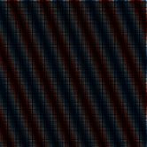
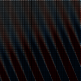
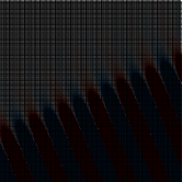
Figure 2: Real part of $\mathrm{EW}_{\varphi,\zeta}$ with $\varphi=\pi/8$, $\zeta\in\{0,1/10,1/2\}$ (left to right) and $\kappa=16$.

5.2 Modal analysis of evanescent plane waves

The Jacobi–Anger expansion (4.3) extends to complex $\mathbf{d}$, i.e. to EPWs, see [31, Eq. (10.12.1), (10.11.1)]: for any $\mathbf{x}=(r,\theta)\in B_{1}$ and $\mathbf{y}=(\varphi,\zeta)\in[0,2\pi)\times\mathbb{R}$,

$$\mathrm{EW}_{\mathbf{y}}(\mathbf{x})=e^{\imath\kappa\mathbf{d}(\mathbf{y})\cdot\mathbf{x}}=\sum_{p\in\mathbb{Z}}\imath^{p}J_{p}(\kappa r)e^{\imath p(\theta-[\varphi+\imath\zeta])}=\sum_{p\in\mathbb{Z}}\left(\imath^{p}e^{-\imath p\varphi}e^{p\zeta}\beta_{p}^{-1}\right)b_{p}(r,\theta).$$ (5.3)

The modulus of the coefficients $\imath^{p}e^{-\imath p\varphi}e^{p\zeta}\beta_{p}^{-1}$ in the modal expansion are reported in Figure 3 (right) as functions of $p$. On this graph, we have conveniently normalized the coefficients according to a normalization factor (depending only on $\zeta$) which is described in the following sections, see (7.11). We see that by tuning the evanescence parameter $\zeta$ we are able to shift the modal content of the plane waves to higher-frequency regimes. As a result, we expect EPWs to be able to capture well the higher-frequency modes of Helmholtz solutions that are less regular. These may arise, for instance, in the presence of close-by singularities. The difficulty then is to properly choose suitable values for this new evanescence parameter $\zeta$ in order to build approximation spaces that are reasonable in size. This will be the main objective of the remainder of this paper.

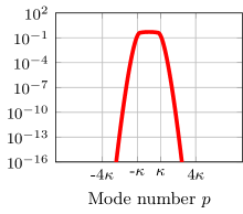
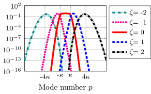
Figure 3: Modal analysis computed using Jacobi–Anger identity (5.3) of $\mathrm{PW}_{\varphi}$ (left) and $\mathrm{EW}_{\varphi,\zeta}$ after normalization (right). In both cases, the absolute values of the coefficients of the expansion of the plane wave in the basis $\{b_{p}\}_{p\in\mathbb{Z}}$ is represented against the mode number $p$. Wavenumber $\kappa=16$. Modifying $\varphi$ has no influence, modifying $\zeta$ shifts the modal content in the Fourier space.

6 Mapping Herglotz densities to Helmholtz solutions

In this section we introduce an integral transform between a space of functions defined on the parametric domain $[0,2\pi)\times\mathbb{R}$ and the space of Helmholtz solutions in the unit disk $\mathcal{B}$.

6.1 Space of Herglotz densities

To shorten notations we denote the parametric domain as the cylinder

$$Y:=[0,2\pi)\times\mathbb{R}.$$ (6.1)

We introduce a weighted $L^{2}$ space defined on $Y$. The weight function is (the square of)

$$w_{z}(\mathbf{y})=w_{z}(\zeta):=e^{-\kappa\sinh|\zeta|+z|\zeta|},\qquad\forall\mathbf{y}=(\varphi,\zeta)\in Y,$$ (6.2)

for some $z\in\mathbb{R}$. In this section, the parameter $z$ is temporarily not specified, although the following analysis shows that it cannot be chosen freely and should take the specific value $z=1/4$, see (6.13). We stress that $w_{z}$ does not depend on the angle $\varphi$. The weighted scalar product and associated norm are then defined by:

$$\left(u,\,v\right)_{\mathcal{A}}:=\int_{Y}u(\mathbf{y})\overline{v(\mathbf{y})}\;w_{z}^{2}(\mathbf{y})\mathrm{d}\mathbf{y},\qquad\qquad\|u\|_{\mathcal{A}}^{2}:=\left(u,\,u\right)_{\mathcal{A}}.$$ (6.3)

We now introduce a subspace of $L^{2}(Y;w_{z}^{2})$ which we call space of Herglotz densities for reasons that will be clear in the following.

Definition 6.1 (Herglotz density).

We define, for any $p\in\mathbb{Z}$,

$$\begin{cases}\tilde{a}_{p}(\mathbf{y}):=e^{p\zeta}e^{\imath p\varphi},\quad\forall\mathbf{y}=\left(\varphi,\zeta\right)\in Y,\\ a_{p}:=\alpha_{p}\tilde{a}_{p},\quad\text{where}\quad\alpha_{p}:=\|\tilde{a}_{p}\|_{\mathcal{A}}^{-1},\end{cases}\quad\text{and}\qquad\mathcal{A}:=\overline{\operatorname{span}\left\{{a}_{p}\right\}_{p\in\mathbb{Z}}}^{\|\cdot\|_{\mathcal{A}}}\subsetneq L^{2}(Y;w_{z}^{2}).$$ (6.4)

The wavenumber $\kappa$ appears explicitly in the weight function $w_{z}$. Therefore, each $a_{p}$ for $p\in\mathbb{Z}$ has an implicit dependence in the wavenumber $\kappa$ through the normalization factor $\alpha_{p}$. Some functions $a_{p}$, weighted by $w_{1/4}$ (see (6.13)), are represented in Figure 4.

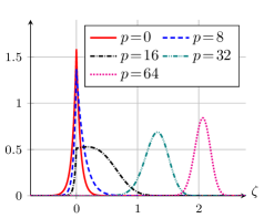
Figure 4: Representation of $\zeta\mapsto|w_{1/4}(\zeta)a_{p}(\zeta,\cdot)|$, which is independent of the second argument of the function $a_{p}$, for mode number $p\in\{0,\kappa/2,\kappa,2\kappa,4\kappa\}$ and wavenumber $\kappa=16$.

For any $p\in\mathbb{Z}$, the complex-valued function $(\zeta+\imath\varphi)\mapsto a_{p}(\varphi,\zeta)$ is a holomorphic function of the complex variable $\zeta+\imath\varphi\in\mathbb{C}$ for any $(\varphi,\zeta)\in Y$. It follows that its real and imaginary parts are harmonic functions on the cylinder $Y$.

Lemma 6.2.

The space $\left(\mathcal{A},\,\|\cdot\|_{\mathcal{A}}\right)$ is a Hilbert space and the family $\{a_{p}\}_{p\in\mathbb{Z}}$ is a Hilbert basis:

$$\left(a_{p},\,a_{q}\right)_{\mathcal{A}}=\delta_{pq},\qquad\forall p,q\in\mathbb{Z},\qquad\text{and}\qquad v=\sum_{p\in\mathbb{Z}}\left(v,\,a_{p}\right)_{\mathcal{A}}a_{p},\qquad\forall v\in\mathcal{A}.$$ (6.5)

The coefficients $\alpha_{p}$ defined in (6.4) decay super-exponentially with $|p|$ after a pre-asymptotic regime up to $|p|\approx\kappa$. The precise asymptotic behavior is given by the following lemma.

Lemma 6.3.

For a constant $c(\kappa)$ only depending on $\kappa$, we have

$$\alpha_{p}\sim c(\kappa)\;\left(\frac{e\kappa}{2}\right)^{|p|}|p|^{1/4-z-|p|}\qquad\text{as}\ |p|\to+\infty.$$ (6.6)

Proof.

It is clear that $\alpha_{-p}=\alpha_{p}$ for all $p\in\mathbb{Z}$. Let $p\in\mathbb{N}$, we have

$$2\pi\int_{-\infty}^{+\infty}e^{2p\zeta+2z|\zeta|}e^{-2\kappa\sinh\left|\zeta\right|}\;\mathrm{d}\zeta =\|\tilde{a}_{p}\|_{\mathcal{A}}^{2} \leq 2\pi\int_{-\infty}^{+\infty}e^{2p|\zeta|+2z|\zeta|}e^{-2\kappa\sinh\left|\zeta\right|}\;\mathrm{d}\zeta,$$ (6.7)

$$2\pi\int_{0}^{+\infty}e^{2(p+z)\zeta}e^{-2\kappa\sinh\zeta}\;\mathrm{d}\zeta \leq\|\tilde{a}_{p}\|_{\mathcal{A}}^{2} \leq 4\pi\int_{0}^{+\infty}e^{2(p+z)\zeta}e^{-2\kappa\sinh\zeta}\;\mathrm{d}\zeta,$$

$$2\pi\kappa^{-m}\int_{\kappa}^{+\infty}\eta^{m-1}e^{-\eta+\frac{\kappa^{2}}{\eta}}\;\mathrm{d}\eta \leq\|\tilde{a}_{p}\|_{\mathcal{A}}^{2} \leq 4\pi\kappa^{-m}\int_{\kappa}^{+\infty}\eta^{m-1}e^{-\eta+\frac{\kappa^{2}}{\eta}}\;\mathrm{d}\eta,$$

$$2\pi\kappa^{-m}\int_{\kappa}^{+\infty}\eta^{m-1}e^{-\eta}\;\mathrm{d}\eta \leq\|\tilde{a}_{p}\|_{\mathcal{A}}^{2} \leq 4\pi e^{\kappa}\kappa^{-m}\int_{\kappa}^{+\infty}\eta^{m-1}e^{-\eta}\;\mathrm{d}\eta,$$

$$2\pi\kappa^{-m}\Gamma(m,\kappa) \leq\|\tilde{a}_{p}\|_{\mathcal{A}}^{2} \leq 4\pi e^{\kappa}\kappa^{-m}\Gamma(m,\kappa),$$

where we used the change of variable $\eta={\kappa}e^{\zeta}$, introduced $m=2(p+z)$ and used the upper incomplete Gamma function defined in [31, Eq. (8.2.2)]. The Gamma function $\Gamma(m)$ and the upper incomplete counterpart $\Gamma(m,\kappa)$ have the same asymptotic behavior for a fixed $\kappa$ when $m$ goes to infinity, see [31, Eq. (8.11.5)] which gives the asymptotic behavior of $1-\Gamma(m,\kappa)/\Gamma(m)$. Using [31, Eq. (5.11.3)] we get $\Gamma(m,\kappa)\sim\Gamma(m)\sim\sqrt{2\pi}e^{-m}m^{m-1/2}$, as $m\to\infty$. We obtain

$$\kappa^{-2(p+z)}\Gamma\big{(}2(p+z),\kappa\big{)}\sim\sqrt{\pi}\left(\frac{2}{e\kappa}\right)^{2(p+z)}\;p^{2(p+z)-1/2}\left(1+\frac{z}{p}\right)^{2(p+z)-1/2}\quad\text{as }p\to+\infty,$$ (6.8)

and the last term is in fact equivalent to $e^{2z}$ at infinity; the claimed result follows. ∎

Using our definitions, the Jacobi–Anger expansion (5.3) takes the simple form

$${\mathrm{EW}_{\mathbf{y}}(\mathbf{x})=\sum_{p\in\mathbb{Z}}\imath^{p}\;\overline{\tilde{a}_{p}(\mathbf{y})}\;\tilde{b}_{p}(\mathbf{x})=\sum_{p\in\mathbb{Z}}\tau_{p}\;\overline{a_{p}(\mathbf{y})}\;b_{p}(\mathbf{x}),\qquad\forall(\mathbf{x},\,\mathbf{y})\in B_{1}\times Y,}$$ (6.9)

where we introduced

$$\tau_{p}:=\imath^{p}\left(\alpha_{p}\beta_{p}\right)^{-1},\qquad\forall p\in\mathbb{Z}.$$ (6.10)

Formula (6.9) relates the basis $\{a_{p}\}_{p\in\mathbb{Z}}$ of the space $\mathcal{A}$ to EPWs $\mathrm{EW}_{\mathbf{y}}$ and circular waves $b_{p}$ on $B_{1}$ and is the key reason for introducing the space $\mathcal{A}$. The behavior of $|\tau_{p}|$ is of crucial importance in the following analysis and is given in Figure 5 for various wavenumber $\kappa$. From the asymptotics given in Lemma 2.4 and Lemma 6.3 we deduce the following result.

Lemma 6.4.

We have

$$|\tau_{p}|\sim c(\kappa)\;|p|^{z-1/4}\qquad\text{as}\ |p|\to+\infty,$$ (6.11)

where the constant $c(\kappa)$ only depends on $\kappa$. Hence, choosing $z=1/4$, we get

$$\tau_{-}:=\inf_{p\in\mathbb{Z}}|\tau_{p}|>0,\qquad\text{and}\qquad\tau_{+}:=\sup_{p\in\mathbb{Z}}|\tau_{p}|<\infty.$$ (6.12)

It is clear that the uniform bounds for $|\tau_{p}|$ are possible only for a precise pair of norms for the space of Helmholtz solutions and the space of Herglotz densities. The bounds $\tau_{\pm}$ depend implicitly on the wavenumber $\kappa$, see Figure 5.

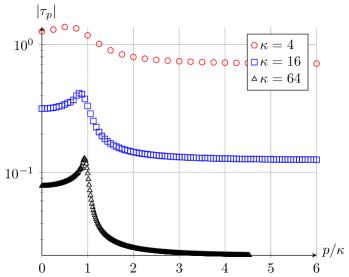
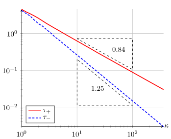
Figure 5: Left: dependence of $|\tau_{p}|$ defined in (6.10) on the mode number $p$ for various wavenumber $\kappa$ and $z=1/4$. Right: dependence of $\tau_{\pm}$ defined in (6.12) on the wavenumber $\kappa$.

The uniform boundedness of $\tau_{p}$ is the key to the following analysis. In the remainder of the paper, we set $z=1/4$ in (6.2) and we let

$$w:=w_{1/4}.$$ (6.13)

We conclude this subsection with a lemma that will be useful in the following.

Lemma 6.5.

For any $\mathbf{x}\in B_{1}$, $\mathbf{y}\mapsto\overline{\mathrm{EW}_{\mathbf{y}}(\mathbf{x})}\in\mathcal{A}$.

Proof.

Let $\mathbf{x}\in B_{1}$ and define $v_{\mathbf{x}}:\mathbf{y}\mapsto\overline{\mathrm{EW}_{\mathbf{y}}(\mathbf{x})}$. The Jacobi–Anger identity (6.9) reads $v_{\mathbf{x}}(\mathbf{y})=\sum_{p\in\mathbb{Z}}\overline{\tau_{p}}\;\overline{b_{p}(\mathbf{x})}\;a_{p}(\mathbf{y})$ for all $\mathbf{y}\in Y$. Since $\{a_{p}\}_{p\in\mathbb{Z}}$ is a Hilbert basis for $\mathcal{A}$, if we write $\mathbf{x}=(r,\theta)\in[0,1)\times[0,2\pi)$, we get

$$\|v_{\mathbf{x}}\|_{\mathcal{A}}^{2}=\sum_{p\in\mathbb{Z}}|\tau_{p}b_{p}(\mathbf{x})|^{2}\leq\tau_{+}^{2}\sum_{p\in\mathbb{Z}}\beta_{p}^{2}|J_{p}(\kappa r)|^{2}.$$ (6.14)

Using the estimates (2.4) and (A.10) from the proof of Lemma 2.4, we get

$$\beta_{p}^{2}|J_{p}(\kappa r)|^{2}\sim\frac{\kappa^{2}}{2\pi}\frac{r^{2|p|}}{|p|},\qquad\text{as}\ |p|\to+\infty,$$ (6.15)

from which we conclude that $\|v_{\mathbf{x}}\|_{\mathcal{A}}<\infty$. ∎

If $\mathbf{x}\in\partial B_{1}$, so that $r=|\mathbf{x}|=1$, then $\mathbf{y}\mapsto\overline{\mathrm{EW}_{\mathbf{y}}(\mathbf{x})}$ does not belong to $\mathcal{A}$, as is readily seen from the proof of Lemma 6.5.

6.2 Herglotz transform

We introduce an integral operator $T$ that allows to write every Helmholtz solution in $\mathcal{B}$ as a continuous linear combination of EPWs weighted by an element of $\mathcal{A}$. We also describe its adjoint operator $T^{*}$, the corresponding frame and Gram operators $S$ and $G$, and prove some of their properties. The terminology of this section is borrowed from Frame Theory, see [12] for a reference on this field.

Synthesis operator.

The first and most important definition concerns the transform that maps Herglotz densities to Helmholtz solutions as we prove next.

Definition 6.6.

Using the weight (6.13), we introduce the Herglotz transform $T$: for any $v\in\mathcal{A}$,

$$\boxed{(Tv)(\mathbf{x}):=\int_{Y}v(\mathbf{y})\mathrm{EW}_{\mathbf{y}}(\mathbf{x})\;w^{2}(\mathbf{y})\mathrm{d}\mathbf{y},\qquad\forall\mathbf{x}\in B_{1}.}$$ (6.16)

This operator is well-defined on $\mathcal{A}$ thanks to Lemma 6.5. In the setting of continuous-frame theory, see e.g. [12, Eq. (5.27)], this operator is called synthesis operator.

The Herglotz transform $T$ is bounded and invertible between the space of Herglotz densities $\mathcal{A}$ and the space of Helmholtz solutions $\mathcal{B}$.

Theorem 6.7.

The operator $T$ is bounded and invertible from $\mathcal{A}$ to $\mathcal{B}$:

$$T\;:\;\mathcal{A}\to\mathcal{B},\quad v\mapsto\sum_{p\in\mathbb{Z}}\tau_{p}\left(v,\,a_{p}\right)_{\mathcal{A}}b_{p},\\ \quad\text{and}\quad\tau_{-}\|v\|_{\mathcal{A}}\leq\|Tv\|_{\mathcal{B}}\leq\tau_{+}\|v\|_{\mathcal{A}}\ \forall v\in\mathcal{A}.$$ (6.17)

Moreover, $Ta_{p}=\tau_{p}b_{p}$ for all $p\in\mathbb{Z}$.

Proof.

Using the Jacobi–Anger formula (6.9), for any $v\in\mathcal{A}$ and $\mathbf{x}\in B_{1}$ we get

$$(Tv)(\mathbf{x}) =\int_{Y}\mathrm{EW}_{\mathbf{y}}(\mathbf{x})v(\mathbf{y})\;w^{2}(\mathbf{y})\mathrm{d}\mathbf{y}=\int_{Y}\left(\sum_{p\in\mathbb{Z}}\tau_{p}\;b_{p}(\mathbf{x})\overline{a_{p}(\mathbf{y})}\right)\;v(\mathbf{y})\;w^{2}(\mathbf{y})\mathrm{d}\mathbf{y}$$ (6.18)

$$=\sum_{p\in\mathbb{Z}}\tau_{p}\int_{Y}\overline{a_{p}(\mathbf{y})}\;v(\mathbf{y})\;w^{2}(\mathbf{y})\mathrm{d}\mathbf{y}\;b_{p}(\mathbf{x})=\sum_{p\in\mathbb{Z}}\tau_{p}\left(v,\,a_{p}\right)_{\mathcal{A}}b_{p}(\mathbf{x}).$$

Hence, from Lemma 2.2, $\|Tv\|_{\mathcal{B}}^{2}=\sum_{p\in\mathbb{Z}}|\tau_{p}|^{2}|\left(v,\,a_{p}\right)_{\mathcal{A}}|^{2},$ and the result (6.17) follows from Lemma 6.2 and Lemma 6.4. It is readily checked that the inverse is given, for any $u\in\mathcal{B}$, by

$$T^{-1}u=\sum_{p\in\mathbb{Z}}\tau_{p}^{-1}\left(u,\,b_{p}\right)_{\mathcal{B}}a_{p}.$$ (6.19)

∎

From (6.19), the inverse operator $T^{-1}$ can also be written as an integral operator: for $u\in\mathcal{B}$,

$$(T^{-1}u)(\mathbf{y})= \int_{B_{1}}u(\mathbf{x})\Psi(\mathbf{x},\mathbf{y})\;\mathrm{d}\mathbf{x}+\kappa^{-2}\int_{B_{1}}\nabla u(\mathbf{x})\cdot\nabla\Psi(\mathbf{x},\mathbf{y})\;\mathrm{d}\mathbf{x},\qquad\forall\mathbf{y}\in Y,$$

$$\text{where }\;\Psi(\mathbf{x},\mathbf{y}):= \sum_{p\in\mathbb{Z}}\tau_{p}^{-1}a_{p}(\mathbf{y})\overline{b_{p}(\mathbf{x})}\qquad\forall\mathbf{x}\in B_{1},\;\mathbf{y}\in Y.$$

The integral representation $Tv$ in (6.16) is similar to the Herglotz representation (4.4). This is the reason why we refer to elements of $\mathcal{A}$ as Herglotz densities. For any $p\in\mathbb{Z}$, the Herglotz densities $\tau_{p}^{-1}a_{p}$ of the circular waves $b_{p}$ are bounded in the $\mathcal{A}$-norm by $\tau_{-}^{-1}$, hence uniformly with respect to the index $p$. This should be contrasted with the standard Herglotz representation (4.8) using only PPWs, where the associated Herglotz densities cannot be bounded uniformly with respect to the index $p$ in $L^{2}([0,2\pi])$. As we explained in Section 4.2, not all Helmholtz solutions admit a bounded Herglotz representation that uses only PPWs (4.4) (with density $v\in L^{2}([0,2\pi])$). In contrast, using EPWs the generalized Herglotz representation (6.16) can represent any Helmholtz solution. Indeed, since $T$ is an isomorphism between $\mathcal{A}$ and $\mathcal{B}$, for any $u\in\mathcal{B}$, there exists a unique $v\in\mathcal{A}$ such that $u=Tv$. The price to pay for this result is the need for a two-dimensional parameter domain, the cylinder $Y$, in place of a one-dimensional one, the interval $[0,2\pi)$, and thus of a double integral; the added dimension corresponds to the evanescence parameter $\zeta$.

Theorem 6.7 is a stability result stated at the continuous level. Next, we aim to obtain a discrete version of this integral representation.

Analysis operator.

In the continuous-frame setting, see [12, Eq. (5.28)], the adjoint operator $T^{*}$ of $T$ is called analysis operator.

Lemma 6.8.

The adjoint $T^{*}$ of $T$ is given for any $u\in\mathcal{B}$ by $(T^{*}u)(\mathbf{y}):=\left(u,\,\mathrm{EW}_{\mathbf{y}}\right)_{\mathcal{B}}$, $\forall\mathbf{y}\in Y$. The operator $T^{*}$ is bounded and invertible on $\mathcal{B}$:

$$T^{*}\;:\;\mathcal{B}\to\mathcal{A},\ u\mapsto\sum_{p\in\mathbb{Z}}\overline{\tau_{p}}\left(u,\,b_{p}\right)_{\mathcal{B}}a_{p},\quad\text{and}\quad\tau_{-}\|u\|_{\mathcal{B}}\leq\|T^{*}u\|_{\mathcal{A}}\leq\tau_{+}\|u\|_{\mathcal{B}},\quad\forall u\in\mathcal{B}.$$ (6.20)

Proof.

We have, for any $v\in\mathcal{A}$ and $u\in\mathcal{B}$

$$\left(Tv,\,u\right)_{\mathcal{B}} =\left(\int_{Y}\mathrm{EW}_{\mathbf{y}}v(\mathbf{y})\;w^{2}(\mathbf{y})\mathrm{d}\mathbf{y},\,u\right)_{\mathcal{B}}=\int_{Y}v(\mathbf{y})\left(\mathrm{EW}_{\mathbf{y}},\,u\right)_{\mathcal{B}}\;w^{2}(\mathbf{y})\mathrm{d}\mathbf{y}$$ (6.21)

$$=\left(v,\,\overline{\left(\mathrm{EW}_{\mathbf{y}},\,u\right)_{\mathcal{B}}}\right)_{\mathcal{A}}=\left(v,\,\left(u,\,\mathrm{EW}_{\mathbf{y}}\right)_{\mathcal{B}}\right)_{\mathcal{A}}.$$

In addition, using the Jacobi–Anger formula (6.9), for any $u\in\mathcal{B}$ and $\mathbf{y}\in Y$

$$(T^{*}u)(\mathbf{y})=\left(u,\,\mathrm{EW}_{\mathbf{y}}\right)_{\mathcal{B}}=\bigg{(}u,\,\sum_{p\in\mathbb{Z}}{\tau_{p}}\;\overline{a_{p}(\mathbf{y})}{b_{p}}\bigg{)}_{\mathcal{B}}=\sum_{p\in\mathbb{Z}}\overline{\tau_{p}}\left(u,\,b_{p}\right)_{\mathcal{B}}a_{p}(\mathbf{y}).$$ (6.22)

From Lemma 2.2, $\|T^{*}u\|_{\mathcal{A}}^{2}=\sum_{p\in\mathbb{Z}}|\tau_{p}|^{2}|\left(u,\,b_{p}\right)_{\mathcal{B}}|^{2},$ and the result follows from Lemma 6.4. ∎

Frame and Gram operators.

We introduce two other important operators in Frame Theory.

Corollary 6.9.

The frame operator $S:=TT^{*}$ and the Gram operator $G:=T^{*}T$ are bounded, invertible, self-adjoint and positive operators:

$$S:=TT^{*}\;:\;\mathcal{B}\to\mathcal{B},\ u\mapsto\sum_{p\in\mathbb{Z}}|\tau_{p}|^{2}\left(u,\,b_{p}\right)_{\mathcal{B}}b_{p},\quad\text{and}\quad\tau_{-}^{2}\|u\|_{\mathcal{B}}\leq\|Su\|_{\mathcal{B}}\leq\tau_{+}^{2}\|u\|_{\mathcal{B}},\ \forall u\in\mathcal{B},$$ (6.23)

$$G:=T^{*}T\;:\;\mathcal{A}\to\mathcal{A},\ v\mapsto\sum_{p\in\mathbb{Z}}|\tau_{p}|^{2}\left(v,\,a_{p}\right)_{\mathcal{A}}a_{p},\quad\text{and}\quad\tau_{-}^{2}\|v\|_{\mathcal{A}}\leq\|Gv\|_{\mathcal{A}}\leq\tau_{+}^{2}\|v\|_{\mathcal{A}},\ \forall v\in\mathcal{A}.$$

Proof.

This result stems directly from Theorem 6.7 and Lemma 6.8. ∎

The frame operator admits the more explicit formula: for any $u\in\mathcal{B}$,

$$Su(\mathbf{x})=\int_{Y}\left(u,\,\mathrm{EW}_{\mathbf{y}}\right)_{\mathcal{B}}\mathrm{EW}_{\mathbf{y}}(\mathbf{x})\;w^{2}(\mathbf{y})\mathrm{d}\mathbf{y},\qquad\forall\mathbf{x}\in B_{1}.$$ (6.24)

A continuous frame result.

We are now ready to prove that EPWs form a continuous frame for the space of Helmholtz solutions in the unit disk. We recall [12, Def. 5.6.1]: given a complex Hilbert space $\mathcal{H}$ and a measure space $M$ with positive measure $\mu$, a family $\{f_{k}\}_{k\in M}\subset\mathcal{H}$ is called “continuous frame” if, $\forall f\in\mathcal{H}$, $k\mapsto\langle f,f_{k}\rangle$ is measurable in $M$, and $\exists A,B>0$ such that $A\|f\|^{2}\leq\int_{M}|\langle f,f_{k}\rangle|^{2}\mathrm{d}\mu(k)\leq B\|f\|^{2}$.

Theorem 6.10.

The family $\left\{\mathrm{EW}_{\mathbf{y}}\right\}_{\mathbf{y}\in Y}$ is a continuous frame for $\mathcal{B}$. Besides, the optimal frame bounds are $A=\tau_{-}^{2}$ and $B=\tau_{+}^{2}$.

Proof.

We need to verify the definition of a continuous frame, see [12, Def. 5.6.1]. For any $u\in\mathcal{B}$, the measurability of $\mathbf{y}\mapsto\left(u,\mathrm{EW}_{\mathbf{y}}\right)_{\mathcal{B}}=(T^{*}u)(\mathbf{y})$, stems from $T^{*}u\in\mathcal{A}$ according to Lemma 6.8 and $\mathcal{A}\subset L^{2}(Y;w^{2})$. The frame condition, namely

$$A\|u\|_{\mathcal{B}}^{2}\leq\int_{Y}|\left(u,\,\mathrm{EW}_{\mathbf{y}}\right)_{\mathcal{B}}|^{2}\;w^{2}(\mathbf{y})\mathrm{d}\mathbf{y}\leq B\|u\|_{\mathcal{B}}^{2},\qquad\forall u\in\mathcal{B},$$ (6.25)

for some constants $A$ and $B$ is a consequence of the boundedness and positivity of the frame operator $S$ which was established in Corollary 6.9. Indeed, for any $u\in\mathcal{B}$, we have

$$\int_{Y}|\left(u,\,\mathrm{EW}_{\mathbf{y}}\right)_{\mathcal{B}}|^{2}\;w^{2}(\mathbf{y})\mathrm{d}\mathbf{y}=\left(Su,\,u\right)_{\mathcal{B}}=\sum_{p\in\mathbb{Z}}|\tau_{p}|^{2}|\left(u,\,b_{p}\right)_{\mathcal{B}}|^{2},$$ (6.26)

which also establishes the optimality of the claimed frame bounds. ∎

6.3 The reproducing kernel property

The continuous frame result implies additional structure on the Herglotz density space $\mathcal{A}$, which then allows to characterize the preimages of the EPWs under the integral transform $T$. For a general reference on Reproducing Kernel Hilbert Spaces (RKHS), we refer to [32].

Lemma 6.11.

The range of the analysis operator $T^{*}$, i.e. the space $\mathcal{A}$ defined in (6.4), has the reproducing kernel property. The reproducing kernel is given by

$$K(\mathbf{z},\mathbf{y})=K_{\mathbf{y}}(\mathbf{z})=\left(K_{\mathbf{y}},\,K_{\mathbf{z}}\right)_{\mathcal{A}}=\sum_{p\in\mathbb{Z}}\overline{a_{p}(\mathbf{y})}a_{p}(\mathbf{z}),\qquad\forall\mathbf{y},\mathbf{z}\in Y,$$ (6.27)

with pointwise convergence of the series and where $K_{\mathbf{y}}\in\mathcal{A}$ is the (unique) Riesz representation of the evaluation functional at $\mathbf{y}\in Y$, namely

$$v(\mathbf{y})=\left(v,K_{\mathbf{y}}\right)_{\mathcal{A}},\qquad\forall v\in\mathcal{A}.$$ (6.28)

Proof.

Take any $v\in\mathcal{A}$ and let $u\in\mathcal{B}$ such that $v=T^{*}u$, which exists thanks to Lemma 6.8. From Corollary 6.9, we have

$$u=S^{-1}Su=\int_{Y}\left(u,\,\mathrm{EW}_{\mathbf{z}}\right)_{\mathcal{B}}S^{-1}\mathrm{EW}_{\mathbf{z}}\;w^{2}(\mathbf{z})\mathrm{d}\mathbf{z}.$$ (6.29)

Then we obtain the reproducing identity, for any $\mathbf{y}\in Y$

$$v(\mathbf{y}) =(T^{*}u)(\mathbf{y})=\left(u,\,\mathrm{EW}_{\mathbf{y}}\right)_{\mathcal{B}}=\int_{Y}\left(u,\,\mathrm{EW}_{\mathbf{z}}\right)_{\mathcal{B}}\left(S^{-1}\mathrm{EW}_{\mathbf{z}},\,\mathrm{EW}_{\mathbf{y}}\right)_{\mathcal{B}}\;w^{2}(\mathbf{z})\mathrm{d}\mathbf{z}$$ (6.30)

$$=\int_{Y}v(\mathbf{z})\left(S^{-1}\mathrm{EW}_{\mathbf{z}},\,\mathrm{EW}_{\mathbf{y}}\right)_{\mathcal{B}}\;w^{2}(\mathbf{z})\mathrm{d}\mathbf{z}=\left(v,\,K_{\mathbf{y}}\right)_{\mathcal{A}},$$

where we introduced (the Riesz representation of) the evaluation functional at the point $\mathbf{y}$ defined as $K_{\mathbf{y}}(\mathbf{z}):=\left(\mathrm{EW}_{\mathbf{y}},\,S^{-1}\mathrm{EW}_{\mathbf{z}}\right)_{\mathcal{B}}$, $\forall\mathbf{z}\in Y.$ It is a direct consequence of Corollary 6.9 that the kernel admits the series representation (6.27). Alternatively, we refer to [32, Th. 2.4] for a direct proof of this result (valid in the general setting), since $\{a_{p}\}_{p\in\mathbb{Z}}$ is an orthonormal basis for $\mathcal{A}$. ∎

Lemma 6.11 does not stem from any specific property of $\mathcal{A}$ or the EPWs, it follows only from the continuous frame result. The reproducing kernel property implies that pointwise evaluation of elements of $\mathcal{A}$ in the cylinder $Y$ is a continuous operation [32, Def. 1.2]: for all $\mathbf{y}\in Y$ there is $c>0$ such that

$$|v(\mathbf{y})|=|\left(v,K_{\mathbf{y}}\right)_{\mathcal{A}}|\leq c\|v\|_{\mathcal{A}},\qquad\forall v\in\mathcal{A}.$$ (6.31)

Examples of (normalized) evaluation functionals are given in Figure 6.

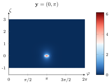
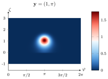
Figure 6: Representation of normalized evaluation functionals $|wK_{\mathbf{y}}|/\|K_{\mathbf{y}}\|_{\mathcal{A}}$ in the cylinder $Y$ for wavenumber $\kappa=16$.

The interest in introducing the reproducing kernel property stems from the following result, which is a direct consequence of Lemma 6.11, Theorem 6.7, and the Jacobi–Anger identity (6.9).

Corollary 6.12.

The EPWs are the images under $T$ of the Riesz representation of the evaluation functionals, namely

$$\mathrm{EW}_{\mathbf{y}}=TK_{\mathbf{y}},\qquad\forall\mathbf{y}\in Y.$$ (6.32)

As a consequence, the construction of an approximation of a Helmholtz solution $u\in\mathcal{B}$ as an expansion of EPWs is, up to the isomorphism $T$, equivalent to the approximation of its Herglotz density $v:=T^{-1}u\in\mathcal{A}$ as an expansion of evaluation functionals, i.e.

$$v\approx\sum_{m=1}^{M}\mu_{m}K_{\mathbf{y}_{m}}\qquad\begin{subarray}{c}T\\ \displaystyle\longrightarrow\\ \displaystyle\longleftarrow\\ T^{-1}\end{subarray}\qquad u\approx\sum_{m=1}^{M}\mu_{m}\mathrm{EW}_{\mathbf{y}_{m}},$$ (6.33)

for some set of coefficients $\boldsymbol{\mu}=\{\mu_{m}\}_{m=1}^{M}$. This remark justifies the use of the sampling techniques described in the next section to discretize the integral representation in (6.16). Section 8 provides numerical evidence that such approximations can be built, for a suitable normalization of the sets $\{K_{\mathbf{y}_{m}}\}_{m}$ and $\{\mathrm{EW}_{\mathbf{y}_{m}}\}_{m}$.

7 A concrete evanescent plane wave approximation set

We describe a method for the numerical approximation of a general Helmholtz solution in the unit disk by EPWs. We exploit the equivalence of this approximation problem with the approximation problem of the corresponding Herglotz density, see (6.33). The main idea is to adapt the sampling procedure of [21, 13, 29] (sometimes called coherence-optimal sampling) to our case, in order to generate a distribution of sampling nodes in the cylinder $Y$ that will be used to reconstruct the Herglotz density. While the numerical recipe that we describe below is found to be numerically very effective, see Section 8, our theoretical analysis still lacks a formal proof of the accuracy and stability of the approximation of Helmholtz solutions using EPWs.

Let $u\in\mathcal{B}$ be the Helmholtz solution, target of the approximation problem, and let $v:=T^{-1}u\in\mathcal{A}$ be its associated Herglotz density. Let also some tolerance $\eta>0$ be given.

7.1 Truncation of the modal expansion

Since $u$ (resp. $v$) a priori lives in an infinite dimensional space $\mathcal{B}$ (resp. $\mathcal{A}$), the idea behind the construction of finite dimensional approximation sets is to exploit the natural hierarchy of finite dimensional subspaces constructed by truncation of the Hilbert basis $\left\{{b}_{p}\right\}_{p\in\mathbb{Z}}$.

Truncation in the Helmholtz solution space.

For any $P\in\mathbb{N}$, we define

$$\mathcal{B}_{P}:=\operatorname{span}\left\{{b}_{p}\right\}_{|p|\leq P}\subset\mathcal{B},\qquad\text{and}\qquad\Pi_{P}\;:\;\mathcal{B}\to\mathcal{B},\ u\mapsto\sum_{|p|\leq P}\left(u,\,b_{p}\right)_{\mathcal{B}}b_{p}.$$ (7.1)

Here $\Pi_{P}$ is the orthogonal projection from $\mathcal{B}$ onto the finite dimensional subspace $\mathcal{B}_{P}$. A natural approach to compute an approximation of $u\in\mathcal{B}$ is to approximate its projection onto $\mathcal{B}_{P}$, namely

$$u_{P}:=\Pi_{P}u\in\mathcal{B}_{P},\qquad\forall P\in\mathbb{N},$$ (7.2)

for some $P$ large enough. It is immediate that the sequence of projections $\{u_{P}\}_{P\in\mathbb{N}}$ converges to $u$ in $\mathcal{B}$. In particular, we can define for any $\eta>0$

$$P^{*}=P^{*}(u,\eta):=\min\big{\{}P\in\mathbb{N}\;|\;\|u-u_{P}\|_{\mathcal{B}}<\eta\|u\|_{\mathcal{B}}\big{\}}.$$ (7.3)

Unfortunately, it is not possible to compute such a $P^{*}$ in most practical configurations. It may be possible though to give estimates on $P^{*}$, based on some regularity assumption on $u$ and the decay of its coefficients in its modal expansion. For instance, it might be physically realistic to assume that all coefficients of the propagative modes $|p|\leq\kappa$ are $\mathcal{O}(1)$ and the coefficients associated to the subsequent evanescent modes $|p|\geq\kappa$ decay in modulus with a given algebraic or exponential rate.

Truncation in the Herglotz density space.

Similarly, for any $P\in\mathbb{N}$, we define

$$\mathcal{A}_{P}:=\operatorname{span}\left\{{a}_{p}\right\}_{|p|\leq P}=T^{-1}\mathcal{B}_{P}\subset\mathcal{A},\qquad\text{and}\qquad v_{P}:=T^{-1}u_{P}\in\mathcal{A}_{P},\qquad\forall P\in\mathbb{N}.$$ (7.4)

Theorem 6.7 implies that the sequence $\{v_{P}\}_{P\in\mathbb{N}}$ converges to $v$ in $\mathcal{A}$. In particular, for any $P\geq P^{*}$, where $P^{*}$ was defined in (7.3), we have

$$\|v-v_{P}\|_{\mathcal{A}}\leq\tau_{-}^{-1}\|u-u_{P}\|_{\mathcal{B}}<\tau_{-}^{-1}\eta\|u\|_{\mathcal{B}}.$$ (7.5)

7.2 Parameter sampling in the cylinder $Y$

Our objective is to approximate the truncated Fourier series $u_{P}=\Pi_{P}u\in\mathcal{B}_{P}$ for some $P\in\mathbb{N}$, instead of $u$. Up to the Herglotz transform, this problem is equivalent to the approximation of $v_{P}=T^{-1}u_{P}\in\mathcal{A}_{P}$. In this subsection let us fix a $P\in\mathbb{N}$, not necessarily equal to $P^{*}$. We propose to build approximations of elements of $\mathcal{A}_{P}$ (resp. $\mathcal{B}_{P}$) by constructing a finite set of sampling nodes $\{\mathbf{y}_{m}\}_{m}$ in the cylinder $Y$ according to the distribution advocated in [21, Sec. 2.1], [13, Sec. 2.2] and [29, Sec. 2]. Despite having an unbounded parametric domain $Y$, the finite integrability of the weight function $w^{2}$ allows to sample $Y$ on a bounded region only. The associated set of sampling functionals $\{K_{\mathbf{y}_{m}}\}_{m}$ (up to some normalization factor) is expected to provide a good approximation of $v_{P}$. The approximation set for $u_{P}$ will then be given by the EPWs $\{\mathrm{EW}_{\mathbf{y}_{m}}\}_{m}$ (up to some normalization factor).

We denote the dimension of both spaces $\mathcal{A}_{P}$ and $\mathcal{B}_{P}$ by

$$N_{P}:=\dim\mathcal{B}_{P}=\dim\mathcal{A}_{P}=2P+1.$$ (7.6)

The probability density function $\rho_{P}$ is defined (up to normalization) as the reciprocal of the $N_{P}$-term Christoffel function $\mu_{P}$ in the spirit of [13, Eq. (2.6)]:

$$\rho_{P}:=\frac{w^{2}}{N_{P}\mu_{P}},\quad\text{where}\quad\mu_{P}(\mathbf{y}):=\Big{(}\sum_{|p|\leq P}|a_{p}(\mathbf{y})|^{2}\Big{)}^{-1},\qquad\forall\mathbf{y}=(\zeta,\varphi)\in Y.$$ (7.7)

Observe that $\rho_{P}$ and $\mu_{P}$ are well-defined since $0<\mu_{P}\leq\mu_{0}<\infty$ from the fact that $a_{0}$ is just a non-vanishing constant. The density function $\rho_{P}$ is a univariate function on $Y$ since it is independent of the angle $\varphi$. We point out that $1/\mu_{P}$ corresponds to the truncated series expansion of the diagonal of the reproducing kernel $K$, which amounts to taking $\mathbf{z}=\mathbf{y}$ and truncating at $P$ the series in (6.27).

The numerical recipe consists, for each $P\in\mathbb{N}$, in generating a sequence of sampling node sets in the parametric domain $Y$

$$\mathbb{Y}_{P}:=\{\mathbb{Y}_{P,M}\}_{M\in\mathbb{N}},\qquad\text{where}\qquad\mathbb{Y}_{P,M}:=\{\mathbf{y}_{m}\}_{m=1}^{M},\quad\forall M\in\mathbb{N},$$ (7.8)

using one’s preferred sampling strategy such that $|\mathbb{Y}_{P,M}|=M$ for all $M\in\mathbb{N}$ and the sequence $\mathbb{Y}_{P}$ converges (in a suitable sense) to the density $\rho_{P}$ defined in (7.7) as $M$ tends to infinity. The sampling method could be a deterministic, a random or even a quasi-random strategy, see Section 8. The sets are not assumed to be nested.

This choice of EPW parameters is a major difference from the heuristic choice described in [24, Eq. (5)] where the parameters are chosen in order to approximate solutions defined in a rectangle containing the physical domain of interest ($B_{1}$ in our case).

7.3 Evanescent plane wave approximation sets

From the sampling node sets (7.8) we can construct two approximations sets: one set of sampling functionals in $\mathcal{A}$ and one set of EPWs in $\mathcal{B}$.

Approximation sets in the Herglotz density space.

Associated to the sampling node sets (7.8), we introduce a sequence of finite sets in $\mathcal{A}$

$$\boldsymbol{\Psi}_{P}:=\{\boldsymbol{\Psi}_{P,M}\}_{M\in\mathbb{N}}\quad\text{where}\quad\boldsymbol{\Psi}_{P,M}:=\left\{\sqrt{\frac{\mu_{P}(\mathbf{y}_{m})}{M}}K_{\mathbf{y}_{m}},\right\}_{\mathbf{y}_{m}\in\mathbb{Y}_{P,M}}\quad\forall M\in\mathbb{N}.$$ (7.9)

The normalization of $K_{\mathbf{y}_{m}}$ in (7.9) is crucial for the stable approximation property (3.3). In the approximation sets, each sampling functional $K_{\mathbf{y}_{m}}$ has been normalized by the real constant $\sqrt{\mu_{P}(\mathbf{y}_{m})/M}$ which is (numerically) close to $\|K_{\mathbf{y}_{m}}\|_{\mathcal{A}}^{-1}/\sqrt{M}$. More precisely, we have

$${\sqrt{\mu_{P}(\mathbf{y})}}\;{\|K_{\mathbf{y}}\|_{\mathcal{A}}}=\Big{(}\sum_{|p|\leq P}|a_{p}(\mathbf{y})|^{2}\Big{)}^{-1/2}\Big{(}\sum_{p\in\mathbb{Z}}|a_{p}(\mathbf{y})|^{2}\Big{)}^{1/2}\geq 1\qquad\forall\mathbf{y}\in Y.$$ (7.10)

Approximation sets in the Helmholtz solution space.

Associated to the sampling set sequences (7.8) and approximation set sequences (7.9) in $\mathcal{A}$, we define the sequence of approximation sets of (normalized) EPWs in $\mathcal{B}$ as follows

$$\boldsymbol{\Phi}:=\{\boldsymbol{\Phi}_{P,M}\}_{P\in\mathbb{N},M\in\mathbb{N}},\qquad\boldsymbol{\Phi}_{P,M}:=\left\{\sqrt{\frac{\mu_{P}(\mathbf{y}_{m})}{M}}\mathrm{EW}_{\mathbf{y}_{m}}\right\}_{\mathbf{y}_{m}\in\mathbb{Y}_{P,M}}\quad\forall P\in\mathbb{N},M\in\mathbb{N}.$$ (7.11)

Following Corollary 6.12, the sequence of sets (7.11) is the image of the sequence of sets (7.9) by the Herglotz transform operator $T$.

Discussion on the parameters.

Our numerical recipe for building the approximation sets $\boldsymbol{\Phi}_{P,M}$ is based on only two parameters, $P$ and $M$, whose tuning is intuitive:

1. The first one is the Fourier truncation parameter $P$. Increasing $P$ will improve the accuracy of the approximation of $u$ (resp. $v=T^{-1}u$) by $u_{P}=\Pi_{P}u$ (resp. $v_{P}=T^{-1}u_{P}$). The appropriate value for $P\geq P^{*}$ will solely depend on the decay of the coefficients in the modal expansion, which is intimately linked to the regularity of the Helmholtz solution.

2. The second one is the dimension $M$ of the EPW approximation space, which is also the number of sampling points in the parameter cylinder $Y$. For a fixed $P$, increasing $M$ should allow to control the accuracy of the approximation of $u_{P}$ (resp. $v_{P}=T^{-1}u_{P}$) by $\mathcal{T}_{\boldsymbol{\Phi}_{P,M}}{\boldsymbol{\xi}}$ (resp. $\mathcal{T}_{\boldsymbol{\Psi}_{P,M}}{\boldsymbol{\xi}}$) for some bounded coefficients $\boldsymbol{\xi}\in\mathbb{C}^{M}$. The numerical results presented below corroborate this conjecture and show experimentally that $M$ should scale linearly with $P$, with a moderate proportionality constant (see Section 8.5).

For a fixed DOF budget $M$, the numerical experiments in Section 8.5 suggests that using a Fourier truncation parameter $P=\max\left(\lceil\kappa\rceil,\lfloor M/4\rfloor\right)$ gives accurate and reliable approximations.

Once the approximation sets $\boldsymbol{\Phi}_{P,M}$ are chosen, our concrete implementation (see Section 3.3) to compute a particular set of coefficients $\boldsymbol{\xi}_{S,\epsilon}$ includes two additional parameters, $S$ and $\epsilon$:

1. The first parameter $S$ is the number of sampling points on the boundary of the physical domain $B_{1}$. According to (B.1) and following [1, 2], sufficient oversampling should be used. In practice, we chose for simplicity an oversampling ratio of $2$, namely $S=2M$. This amount of oversampling may not be necessary and further numerical experiments could investigate a reduction of the oversampling ratio $S/M$ to reduce the computational cost.

2. The second parameter $\epsilon$ is the regularization parameter, i.e. the truncation threshold of the singular values. We set this parameter to $\epsilon=10^{-14}$ in the numerical experiments presented below. If one is interested in less accurate approximations than ours, this parameter could be set to larger values.

We stress that the construction of the approximation sets $\boldsymbol{\Phi}_{P,M}$, together with their accuracy and stability, are not influenced by the choice of the reconstruction strategy made in Section 3.2. Although we focus on the simple method of boundary sampling together with regularized SVD, alternative reconstruction strategies (such as sampling in the bulk of the domain or taking inner product with elements of other types of test spaces, for instance) and other regularization techniques (such as Tikhonov regularization) can also be successfully used in practice. Irrespective of the strategy, sufficient oversampling and regularization need to be used.

Relation with the literature.

As we have already alluded to, our construction is based on similar ideas that pre-exist in the literature but in a different context. Indeed, sampling node sets similar to the ones we propose here can be found in [21, 13, 29]. The context of these works is the reconstruction of elements of finite-dimensional subspaces (with explicit orthonormal basis) in weighted $L^{2}$ spaces from sampling [13] and it was subsequently used to construct random cubature rules [29]. The underlying idea is that the information gathered from sampling at these nodes is enough to allow accurate reconstruction as an expansion in the (truncated) orthonormal basis.

Translated into our setting, the results available in the literature say that to reconstruct an element $v_{P}=\Pi_{P}v$ of the finite dimensional subspace $\mathcal{A}_{P}$, it is enough to sample at the nodes $\boldsymbol{\Psi}_{P,M}$ for some sufficiently large $M$. In contrast, the numerical recipe described above seeks to construct an approximation of the element $v_{P}=\Pi_{P}v\in\mathcal{A}_{P}$ as an expansion in the set of evaluation functionals $\boldsymbol{\Psi}_{P,M}$ for some sufficiently large $M$. In other words, the approximation we are looking for belongs to the span of the evaluation functionals, $\operatorname{span}\boldsymbol{\Psi}_{P,M}$, which has trivial intersection with $\mathcal{A}_{P}$. By Corollary 6.12, applying the Herglotz transform $T$ to this approximation in $\operatorname{span}\boldsymbol{\Psi}_{P,M}$ yields an element in $\operatorname{span}\boldsymbol{\Phi}_{P,M}$ (i.e. a finite superposition of EPWs) that approximates $u_{P}=Tv_{P}\in\mathcal{B}_{P}$.

Unfortunately, besides the links with these works, we are not yet able to prove a rigorous theoretical analysis to support our numerical recipe. Yet, extensive numerical experiments in Section 8 illustrate the excellent approximation and stability properties of the sets $\boldsymbol{\Phi}_{P,M}$.

7.4 A conjectural stable approximation result

We formalize below our speculations, which are hinted by the numerical experiments given in the next section. First, we state our main conjecture.

Conjecture 7.1.

The sequence of approximation sets $\boldsymbol{\Psi}_{P}$ defined in (7.9) is a stable approximation for $\mathcal{A}_{P}$, in the following sense: there exist $s\geq 0$ and $C>0$ such that, for all $P\in\mathbb{N}$, there exists $M^{*}=M(P,\eta)$ such that

$$\forall v_{P}\in\mathcal{A}_{P},\ \exists M\in\mathbb{N},\ \boldsymbol{\mu}\in\mathbb{C}^{M},\quad\|v_{P}-\mathcal{T}_{\boldsymbol{\Psi}_{P,M}}{\boldsymbol{\mu}}\|_{\mathcal{A}}\leq\eta\|v_{P}\|_{\mathcal{A}}\ \ \text{and}\ \ \|\boldsymbol{\mu}\|_{\ell^{2}}\leq CM^{s}\|v_{P}\|_{\mathcal{A}}.$$ (7.12)

In the following we assume for simplicity that all $M\geq M^{*}$ satisfy the two inequalities appearing in (7.12) (otherwise the proofs can be easily adapted). This holds true if the sets are hierarchical, for instance, but this is not necessary.

Provided the above conjecture holds, the stability of the approximation sets of EPWs constructed above would follow as we prove next.

Proposition 7.2.

Let $\delta>0$. If Conjecture 7.1 holds then the sequence of approximation sets (7.11) provides a stable approximation for $\mathcal{B}$. In particular, if $\kappa^{2}$ is not a Dirichlet eigenvalue on $B_{1}$,

$$\forall u\in\mathcal{B}\cap C^{0}(\overline{B_{1}}),\ \exists P\in\mathbb{N},\ M\in\mathbb{N},\ S\in\mathbb{N},\ \epsilon\in(0,1],\qquad\|u-\mathcal{T}_{\boldsymbol{\Phi}_{P,M}}\boldsymbol{\xi}_{S,\epsilon}\|_{L^{2}(B_{1})}\leq\delta\|u\|_{\mathcal{B}},$$ (7.13)

where $\boldsymbol{\xi}_{S,\epsilon}\in\mathbb{C}^{|\boldsymbol{\Phi}_{P,M}|}$ is computed with the regularization procedure in (3.10). The SVD regularization parameter $\epsilon$ can be chosen as (3.14).

Proof.

We need to prove the stability of the sequence of approximation sets, namely that for any $\tilde{\eta}>0$, there exists $\tilde{s}\geq 0$ and $\tilde{C}>0$ such that

$$\forall u\in\mathcal{B},\ \exists P\in\mathbb{N},\ M\in\mathbb{N},\ \boldsymbol{\mu}\in\mathbb{C}^{M},\quad\|u-\mathcal{T}_{\boldsymbol{\Phi}_{P,M}}{\boldsymbol{\mu}}\|_{\mathcal{B}}\leq\tilde{\eta}\|u\|_{\mathcal{B}}\ \ \text{and}\ \ \|\boldsymbol{\mu}\|_{\ell^{2}}\leq\tilde{C}M^{\tilde{s}}\|u\|_{\mathcal{B}}.$$ (7.14)

Provided this holds, the claimed result is a direct application of Corollary 3.3.

Let $\eta>0$, $u\in\mathcal{B}$ and set $v:=T^{-1}u\in\mathcal{A}$. For any $P\geq P^{*}=P^{*}(u,\eta)$ with $P^{*}$ defined in (7.3), if we let $u_{P}:=\Pi_{P}u$ and $v_{P}:=T^{-1}u_{P}$ we have (recall (7.5))

$$\|u-u_{P}\|_{\mathcal{B}}\leq\eta\|u\|_{\mathcal{B}},\qquad\text{and}\qquad\|v-v_{P}\|_{\mathcal{A}}\leq\tau_{-}^{-1}\eta\|u\|_{\mathcal{B}}.$$ (7.15)

Assuming that Conjecture 7.1 holds, there exist $s$ and $C$ (both independent of $P$) such that, for any $M\geq M^{*}(P^{*},\eta)$, there exists a set of coefficients $\boldsymbol{\mu}\in\mathbb{C}^{M}$ such that

$$\|v_{P}-\mathcal{T}_{\boldsymbol{\Psi}_{P,M}}\boldsymbol{\mu}\|_{\mathcal{A}}\leq\eta\|v_{P}\|_{\mathcal{A}},\qquad\text{and}\qquad\|\boldsymbol{\mu}\|_{\ell^{2}}\leq CM^{s}\|v_{P}\|_{\mathcal{A}}.$$ (7.16)

The properties of the isomorphism $T$ given in Theorem 6.7 imply that

$$\|u_{P}-\mathcal{T}_{\boldsymbol{\Phi}_{P,M}}\boldsymbol{\mu}\|_{\mathcal{B}}<\tau_{+}\eta\|v_{P}\|_{\mathcal{A}}\qquad\text{and}\qquad\|v_{P}\|_{\mathcal{A}}\leq\tau_{-}^{-1}\|u_{P}\|_{\mathcal{B}}\leq\tau_{-}^{-1}\|u\|_{\mathcal{B}}.$$ (7.17)

For any $P\geq P^{*}(u,\eta)$ and $M\geq M^{*}(P^{*},\eta)$, the total approximation error for the Herglotz density $v$ can be estimated as

$$\|v-\mathcal{T}_{\boldsymbol{\Psi}_{P,M}}\boldsymbol{\mu}\|_{\mathcal{A}}\leq\|v-v_{P}\|_{\mathcal{A}}+\|v_{P}-\mathcal{T}_{\boldsymbol{\Psi}_{P,M}}\boldsymbol{\mu}\|_{\mathcal{A}}\leq 2\tau_{-}^{-1}\eta\|u\|_{\mathcal{B}},$$ (7.18)

and for the Helmholtz solution $u$ as

$$\begin{aligned} \|u-\mathcal{T}_{\boldsymbol{\Phi}_{P,M}}\boldsymbol{\mu}\|_{\mathcal{B}}&\leq\|u-u_{P}\|_{\mathcal{B}}+\|u_{P}-\mathcal{T}_{\boldsymbol{\Phi}_{P,M}}\boldsymbol{\mu}\|_{\mathcal{B}}\\ &\leq\left(1+\tau_{+}\tau_{-}^{-1}\right)\eta\|u\|_{\mathcal{B}},\end{aligned}\qquad\text{and}\qquad\|\boldsymbol{\mu}\|_{\ell^{2}}\leq CM^{s}\tau_{-}^{-1}\|u\|_{\mathcal{B}}.$$ (7.19)

Choosing $\eta=\tilde{\eta}/(1+\tau_{+}\tau_{-}^{-1})$, we can conclude since (7.19) is (7.14) with $\tilde{s}=s$ and $\tilde{C}=C\tau_{-}^{-1}$. ∎

8 Numerical results

We provide numerical evidence that the procedure described above allows to compute controllably accurate approximations of Helmholtz solutions in the unit disk and in other domains.

8.1 Probability densities and samples

Probability density and cumulative distributions functions.

We represent the probability density function $\rho_{P}$ (see (7.7)) as a function of the evanescence parameter $\zeta$ on the left in Figure 7. Here $P$ denotes the truncation parameter, meaning that the sampling is performed to approximate elements of $\mathcal{A}_{P}$, which has dimension $N_{P}$. The associated cumulative distribution function with respect to the evanescence parameter $\zeta$ is defined as

$$\Upsilon_{P}(\zeta):=\int_{-\infty}^{\zeta}\rho_{P}(\tilde{\zeta})\;\mathrm{d}\tilde{\zeta},\qquad\forall\zeta\in\mathbb{R}.$$ (8.1)

It is represented in the right of Figure 7. Recall that while $\rho_{P}$ is a bi-variate function on the cylinder $Y$, it is constant with respect to the angle $\varphi$. As a result, the cumulative distribution with respect to this variable $\varphi$ is a linear function. This is why we represent these two functions $\rho_{P}$ and $\Upsilon_{P}$ only with respect to the evanescence parameter $\zeta$.

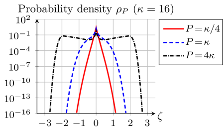
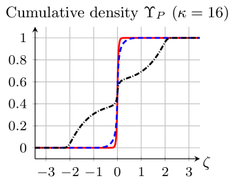
Figure 7: Sampling density functions $\rho_{P}$ (left) and $\Upsilon_{P}$ (right) with respect to the evanescence parameter $\zeta$ constructed for the subspace $\mathcal{A}_{P}$. Wavenumber $\kappa=16$.

We observe that the probability density $\rho_{P}$ is a symmetric even function and exhibits a main mode at $\zeta=0$ which corresponds to purely PPWs. Moreover, the $\epsilon$-support of this density is rather tight and the probability eventually tends to zero exponentially as $|\zeta|$ gets large enough. When $P\leq\kappa$ the density is a unimodal distribution whereas for $P\gg\kappa$ (e.g. $P=4\kappa$) the density is a multimodal distribution. Indeed, in the latter case, there are two symmetric modes for relatively large evanescence parameter, in addition to the main mode at $\zeta=0$. The cumulative distribution function $\Upsilon_{P}$ is close to a step function in the case where $\mathcal{A}_{P}$ contains only elements associated to the propagative regime $P\leq\kappa$. In contrast, for $P>\kappa$ the distribution is non-trivial for moderate values of the evanescence parameter $\zeta$. This means that for $P\leq\kappa$ one can safely choose only PPWs, while for $P>\kappa$ EPWs are needed and their choice is non-trivial.

Parameter sampling.

For any $P$ we generate $M=\nu N_{P}$ samples in the cylinder $Y$ using the technique called Inversion Transform Sampling (ITS) [13, Sec. 5.2]. It consists in first generating sampling sets in the unit square $[0,1]^{2}$ that converge (in a suitable sense) to the uniform distribution $\mathcal{U}_{[0,1]^{2}}$ when $M\to\infty$,

$$\{\mathbf{z}_{m}\}_{m},\qquad\text{with}\qquad\mathbf{z}_{m}=(z_{m,\varphi},z_{m,\zeta})\in[0,1]^{2},\quad m=1,\ldots,M,$$ (8.2)

and then map back to the cylinder $Y$, to obtain sampling sets that converge to the probability density function $\rho_{P}$ when $M\to\infty$, namely

$$\{\mathbf{y}_{m}\}_{m},\qquad\text{with}\qquad\mathbf{y}_{m}:=\left(2\pi z_{m,\varphi},\Upsilon_{P}^{-1}(z_{m,\zeta})\right)\in Y,\quad m=1,\ldots,M.$$ (8.3)

The fact that the density function is constant with respect to $\varphi$ considerably simplifies the generation of the samples. The inversion $\Upsilon_{P}^{-1}$ can be performed using elementary root-finding techniques, our implementation resorts to the bisection method.

In our numerical experiments we tested three types of sampling methods, which differ by how we generate the first sampling distribution $\{\mathbf{z}_{m}\}_{m}$ in the unit square:

1. deterministic sampling: the initial samples in the unit square are a Cartesian product of two sets of equispaced points with the same number of points in both directions (all numerical results presented are obtained by using as approximation set dimension the smallest square integer larger than or equal to $M$);

2. Sobol sampling: the initial samples in the unit square corresponds to Sobol sequences which are quasi-random low-discrepancy sequences;

3. random sampling: the initial samples in the unit square are drawn randomly according to the product of two uniform distributions $\mathcal{U}_{[0,1]}$.

Some examples of sampling sets corresponding to the probability density function $\rho_{P}$ for $\kappa=16$ are reported in Figure 8. For these examples the number of sampling nodes is set to $M=\nu N_{P}$ with $\nu=4$, for the three types of sampling considered. As expected, the sampling points cluster near the line $\zeta=0$ for smaller $P$. This is the (propagative) regime for which PPWs alone provide a good approximation. When $P>\kappa$ the evanescence parameter $\zeta$ spreads in a wider domain, with some clustering at the secondary modes of the distribution, in agreement with Figure 7.

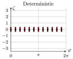
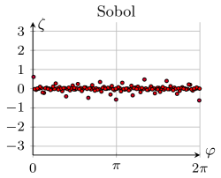
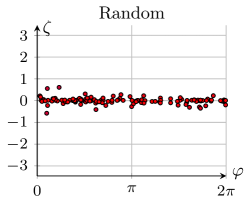
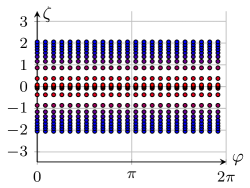
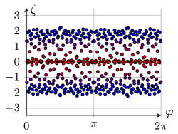
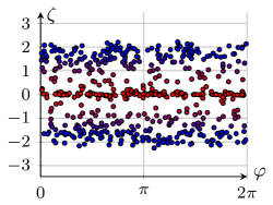
$P=\kappa\$ $P=4\kappa$

Figure 8: $M=4N_{P}$ samples in the cylinder $Y$ for $P=\kappa$ (top) and $P=4\kappa$ (bottom) and various types of sampling method (left to right). Wavenumber $\kappa=16$. Large $|\zeta|$ implies fast EPW decay.

8.2 Propagative plane waves are unstable

Before presenting EPW approximations, we report some numerical experiments dedicated to verifying numerically the instability result of Lemma 4.2 when using PPWs. These will also serve as a reference point to compare with the results obtained using our EPW recipe.

Let us consider the approximation problem of Section 4.3, namely the approximation of the circular wave $b_{p}$ for some $p\in\mathbb{Z}$ by an approximation set $\boldsymbol{\Phi}_{M}$ of $M\in\mathbb{N}$ PPWs defined in (4.2). The sampling matrix $A$ was defined in (3.6), using $M$ PPWs with equispaced angles and $S:=\max(2M,2|p|)$ sampling points (we impose $S\geq 2|p|$ to avoid spurious results due to aliasing). The entries of the matrix $A$ are immediately computed as $A_{s,m}=e^{\imath\kappa\cos(2\pi(\frac{s}{S}-\frac{m}{M}))}$ for $s=1,\ldots,S$, $m=1,\ldots M$. The right-hand side $\mathbf{b}$ is defined as in (3.6) for $b_{p}$ in place of $u$; we recall that we use Dirichlet data in all our numerical experiments.

The matrix $A$ is notoriously ill-conditioned (see Figure 10(a)): its condition number grows exponentially with respect to the number of plane waves $M$ in the approximation set $\boldsymbol{\Phi}_{M}$. This is well-known, see for instance the numerical experiments in [33, Sec. 2.3] for the circular geometry and $S=M$. This is not a feature of the sampling method: we refer to similar experiments in [22, Sec. 4.3] for the mass matrix of a Galerkin formulation in a Cartesian geometry, again for $S=M$. The least-squares formulation suffers from an even worse condition number: proportional to the square of the condition number of the sampling method, see e.g. [33, Eq. (30)]. We apply the regularization procedure described in Section 3.3 with threshold parameter $\epsilon=10^{-14}$.

The numerical results are reported in Figure 9(a). On the left panel we report the relative residual $\mathcal{E}$ defined in (3.15) as a measure of the accuracy of the approximation. On the right panel we report the size of the coefficients $\|\boldsymbol{\xi}_{S,\epsilon}\|_{\ell^{2}}$ as a measure of the stability of the approximation. Relative residuals and coefficient norms were already used in [24] to assess the stability of the approximations.

We observe three regimes. First, for the propagative modes, i.e. the circular waves with mode number $|p|\leq\kappa$, the approximation is accurate ($\mathcal{E}<10^{-13}$) and the size of the coefficients is moderate ($\|\boldsymbol{\xi}_{S,\epsilon}\|<10$). Second, for mode numbers $|p|$ roughly larger than the wavenumber $\kappa$, the norms of the coefficients of the computed approximations blow up exponentially. The accuracy is spoiled proportionally. Third, for evanescent modes with $|p|$ larger than about $2\kappa$ or $3\kappa$, the size of the coefficients completely destroys the stability of the approximation, and we cannot approximate the target $b_{p}$ with any decent accuracy. Of course, for a relative error at $\mathcal{O}(1)$, the coefficient norm reported is not meaningful, and taking $\boldsymbol{\xi}_{S,\epsilon}$ identically zero would provide a similar error.

Increasing the number of plane waves $M$ has no effect on the accuracy beyond a certain point. Indeed, Figure 10(a) shows that the $\epsilon$-rank (i.e. the number of singular values larger than $\epsilon$) of the matrix $A$ does not increase when $M$ is raised. Although increasing $M$ does not bring any higher accuracy, it does not increase any further the numerical instability. For a fixed $M$, the same matrix $A$ is used to approximate all the $b_{p}$’s for any mode number $p$ (i.e. to compute all markers of the same color in Figure 9(a)). Even when the matrix $A$ is extremely ill-conditioned (say $M=32\kappa$ in the numerical experiments presented here), we get at the same time almost machine-precision accuracy for all propagative modes $|p|\leq\kappa$ while having $\mathcal{O}(1)$ error for evanescent modes with larger mode number $|p|\geq 3\kappa$. It is the simple regularization procedure described in Section 3.3 that allows us to obtain such results. No other technique can overcome the inherent instability of PPWs. In particular, even with regularization, accuracy in the approximation of the evanescent modes remains out of reach for a given floating-point precision.

Analoguous numerical results are also observed in the context of the MFS, see [5, Fig. 3].

(a) PPW

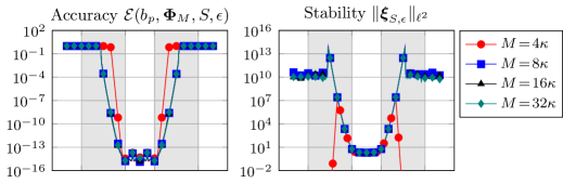
(b) EPW:
deterministic
sampling

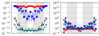
(c) EPW:
Sobol
sampling

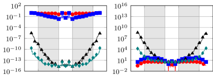
(d) EPW:
random
sampling

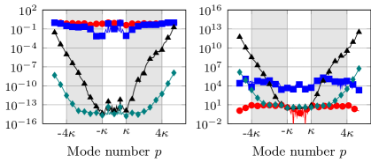
Figure 9: Accuracy $\mathcal{E}$, as defined in (3.15), (left) and stability $\|\boldsymbol{\xi}_{S,\epsilon}\|_{\ell^{2}}$ (right) of the approximation of circular waves $b_{p}$ by PPW (top row) and EPWs (three bottom rows). Truncation at $P=4\kappa$ for EPWs, wavenumber $\kappa=16$. With PPWs, the approximation accuracy does not improve as $M$ increases beyond some value, because of exponentially large (with respect to $p$) coefficients, as proved in Lemma 4.2. With EPWs, the approximation accuracy improves as $M$ increases, thanks to a decrease of the size of the coefficients.

8.3 Evanescent plane waves are stable

We investigate, for the same test cases, whether the EPW sets proposed in Section 7.3 achieve better stability properties while not compromising the accuracy of the approximation. The approximation sets $\boldsymbol{\Phi}_{P,M}$ are defined in (7.11) and the $M$ EPWs have parameters $\{\mathbf{y}_{m}\}_{m=1}^{M}$ computed as in (8.3), i.e. distributed according to the sampling distribution $\rho_{P}$ defined in (7.7). These EPWs are normalized as in (7.11). Here the parameter $P$ used to generate the $M$ samples (which are adapted to the space $\mathcal{A}_{P}$) is set to $4\kappa$. The numerical results are reported in Figure 9.

The main observation is that by using sufficiently many waves (i.e. setting $M$ sufficiently large, on the order of $M=32\kappa\approx 4N_{P}$) we are now able to approximate to (almost) machine precision all the modes $|p|\leq P=4\kappa$. This includes the propagative modes $|p|\leq\kappa$ (which were already well-approximated by purely PPWs), but more importantly, this also includes evanescent modes $\kappa<|p|\leq P=4\kappa$ (corresponding to the greyed out area), for which purely PPWs failed to provide any meaningful approximation. Moreover, even much higher modes $|p|>P=4\kappa$ are approximated to acceptable accuracy. Further, we stress that the norms of the coefficients $\|\boldsymbol{\xi}_{S,\epsilon}\|_{\ell^{2}}$ used in the approximate expansions remain moderate, especially for large $M$. This is in stark contrast with the results of Section 8.2, where the exponential growth of the coefficients prevented any accurate numerical approximation.

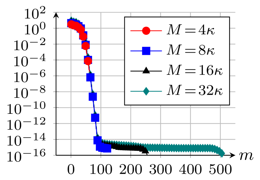
(a) PPW.

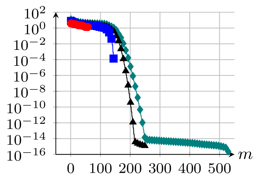
(b) EPW: deterministic sampling

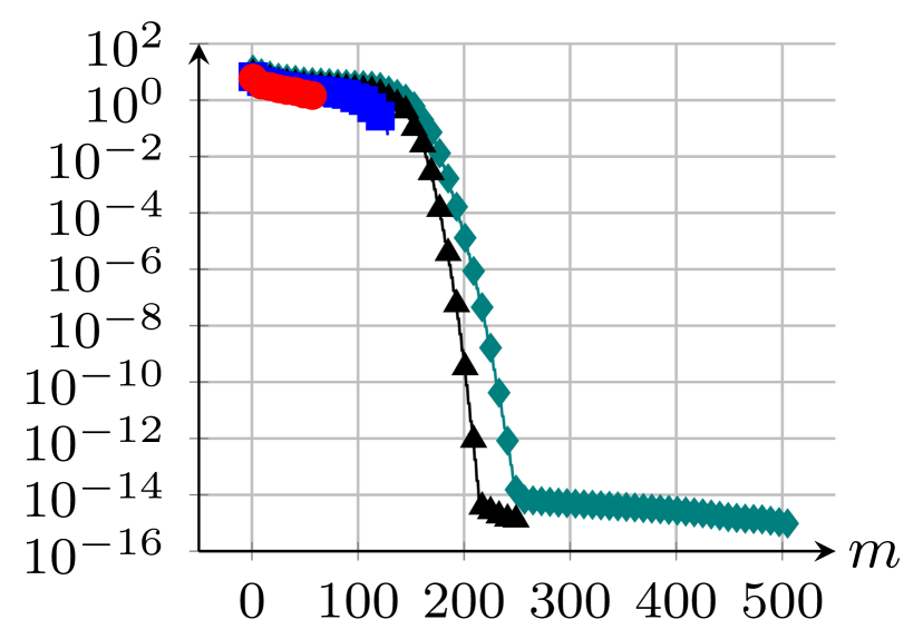
(c) EPW: Sobol sampling

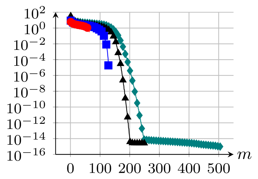
(d) EPW: random sampling

Figure 10: Singular values $\{\sigma_{m}\}_{m=1}^{M}$ of the matrix $A$ when using a set of $M$ plane waves. Truncation at $P=4\kappa$ for EPWs, wavenumber $\kappa=16$. The matrices associated to EPWs are not better conditioned than the ones associated to PPWs, however the number of singular values above the regularization threshold $\epsilon=10^{-14}$ increases with $M$ and $P$.

In Figure 10, we observe that the condition number of the matrix $A$ is of the same order for PPWs and EPWs, when $M$ is large enough. The improved accuracy for evanescent modes is not due to an improved conditioning of the underlying linear system but to an increase of the $\epsilon$-rank of the matrix, i.e. the number of singular values larger than $\epsilon$. This number goes from less than $100$ for PPWs to around $250$ for EPWs in the case $M=32\kappa$. To further increase the $\epsilon$-rank, one needs to increase the truncation parameter $P$.

Comparing PPWs and EPWs, we see that for small $M$ (e.g. $M=4\kappa$ and $M=8\kappa$) purely PPWs provide better approximation of propagative modes than EPWs. This is because the approximation spaces made of PPWs are tuned for propagative modes, which span a space of dimension $2\kappa+1$. In contrast, the approximation spaces made of EPWs target a larger number of modes, including some evanescent modes, which span a space of dimension $N_{P}=2P+1$ with $P=4\kappa$ in this numerical experiment. For a general target solution containing evanescent modes, one does not expect any advantage in using PPWs only.

8.4 Approximation of random-expansion solutions

We test the procedure described so far by reconstructing a solution of the form

$$u:=\sum_{|p|\leq P}\hat{u}_{p}\left[\max\left(1,|p|-\kappa\right)\right]^{-1/2}b_{p}\;\in\mathcal{B}_{P}$$ (8.4)

in which $\hat{u}_{p}$ are normally-distributed random numbers with mean $0$ and standard deviation $1$. The coefficients of any element of $\mathcal{B}$ decay in modulus as $o(|p|^{-1/2})$ for $|p|\to\infty$; this is therefore a rather difficult scenario for an approximation problem.

We then apply the procedure described above for the three types of sampling strategies considered. The sampling points are constructed knowing that $T^{-1}u$ is an element of $\mathcal{A}_{P}$. In other words, the optimal modal truncation parameter $P^{*}=P$ (where $P$ appears in (8.4)) is assumed to be known in this numerical experiment. The main purpose is to investigate the validity of Conjecture 7.1. We study here the convergence of the error with respect to the dimension of the approximation space $M$. The number of sampling points on the boundary of the disk is set to $S=2M$. The numerical results are given in Figure 11 for the Sobol sampling strategy only. On the left panel we report the relative residual $\mathcal{E}$, defined in (3.15), as a measure of the accuracy of the approximation. On the right panel we report the size of the coefficients, namely $\|\boldsymbol{\xi}_{S,\epsilon}\|_{\ell^{2}}/\|u\|_{\mathcal{B}}$, as a measure of the stability of the approximation.

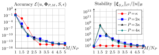
Figure 11: Accuracy $\mathcal{E}$, as defined in (3.15), (left) and stability $\|\boldsymbol{\xi}_{S,\epsilon}\|_{\ell^{2}}/\|u\|_{\mathcal{B}}$ (right) of the approximation by $M$ EPWs (constructed using Sobol sampling) of a solution $u$ in the form (8.4) that belong to the space $\mathcal{B}_{P}$ of dimension $N_{P}=2P+1$. The horizontal axis represents the ratio $M/N_{P}$. Wavenumber $\kappa=16$. The number $M$ of EPWs necessary to approximate elements of the space $\mathcal{B}_{P}$ seems to scale linearly with the space dimension $N_{P}$.

The main observation is that the error quickly decays with respect to the ratio $M/N_{P}=M/(2P+1)$, which represents the ratio of the dimension of the approximation set $M$ over the dimension of the space $\mathcal{B}_{P}$ the solution (8.4) lives in. When $P$ is large enough (say $P\geq 2\kappa$ which remains moderate), the decay is relatively independent of $P$. The second observation is that the norm of the coefficients $\|\boldsymbol{\xi}_{S,\epsilon}\|_{\ell^{2}}/\|u\|_{\mathcal{B}}$ in the expansions is a decreasing function of the size $M$ of the approximation space. We see once more that one gets accurate and stable approximations. The values of $\|\boldsymbol{\xi}_{S,\epsilon}\|_{\ell^{2}}/\|u\|_{\mathcal{B}}$ reported for small values of $M/N_{P}$, and in particular the increase at the start, are not significant since they correspond to inaccurate approximations.

We report in Figure 12 the plots of a solution (8.4) for a larger frequency $\kappa=64$ and truncation parameter $P=3\kappa=192$. The approximation error when using $M=3(2P+1)=1155$ PPWs or EPWs is also given, with points in $Y$ sampled as a Sobol sequence. In the first case the absolute error in the disk is much larger, more than $12$ orders of magnitude larger if measured in $L^{\infty}(B_{1})$ norm, and concentrated near the boundary. The number of degrees of freedom per wavelength $\lambda={2\pi}/{\kappa}$ used in each direction can be estimated by $\lambda\sqrt{{M}/{\pi}}\approx 1.9$. Note that $\pi$ here represents the area of the unit disk. For low-order methods, a common rule of thumb is to use around $6\sim 10$ degrees of freedom per wavelength to have $1$ or $2$ digits of accuracy. We obtain $12$ digits of accuracy for only a fraction of this number. For $M=2(2P+1)=770$, the maximum absolute error reached is measured to $1.3\cdot 10^{-10}$ (not plotted).

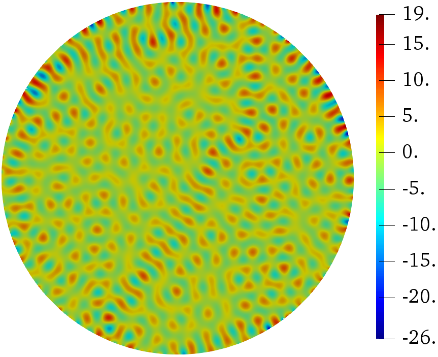
(a) Real part of target solution $\Re u$

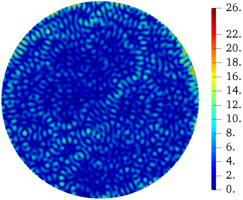
(b) Modulus of target solution $|u|$

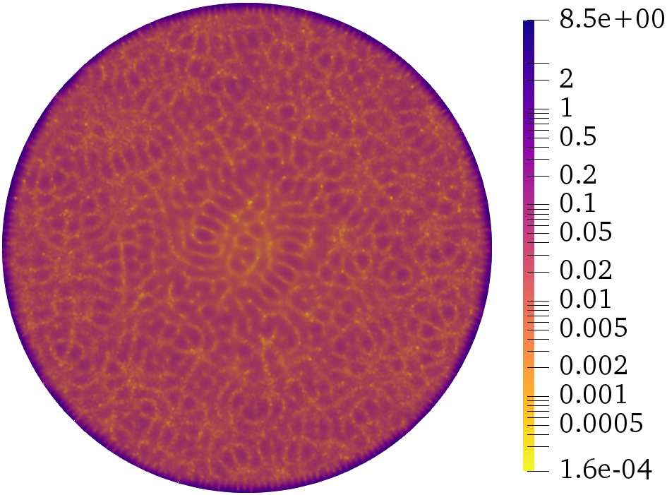
(c) Absolute error using PPW $|u-\mathcal{T}_{\boldsymbol{\Phi}_{M}}\boldsymbol{\xi}_{S,\epsilon}|$

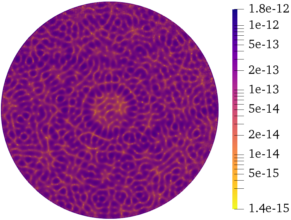
(d) Absolute error using EPW $|u-\mathcal{T}_{\boldsymbol{\Phi}_{P,M}}\boldsymbol{\xi}_{S,\epsilon}|$

Figure 12: Solution $u$, target of the approximation, defined in (8.4) with $P=3\kappa=192$ (top) and associated absolute errors when approximated by $M=3(2P+1)=1155$ plane waves, either propagative ones $\boldsymbol{\Phi}_{M}$ from (4.2) (bottom left) or evanescent ones $\boldsymbol{\Phi}_{P,M}$ from (7.11), whose parameters are constructed using a Sobol type sampling (bottom right). The colormaps associated to absolute errors are logarithmic for better visualization. Wavenumber $\kappa=64$. Note the different color scales, which shows a factor-$10^{12}$ improvement in using EPWs instead of PPWs.

Overall, the numerical results are perfectly consistent with Conjecture 7.1.

8.5 Numerical evidence of quasi-optimality

An important question regarding the efficiency of the proposed method concerns how the size of the approximation set $M$ should vary with respect to the truncation parameter $P$. Fixing $P$ amounts to looking at the finite dimensional subspace $\mathcal{B}_{P}$ which contains the first $N_{P}=2P+1$ modes. Since $N_{P}$ is the dimension of $\mathcal{B}_{P}$ there is no hope to have approximation spaces with dimension $M<N_{P}$ that are able to approximate all elements of this space. An optimal approximation set would therefore achieve this with $M=N_{P}$ elements at best. We show numerical evidence that we achieve quasi-optimality, in the sense that the approximation spaces $\boldsymbol{\Phi}_{P,M}$ defined in (7.11) only need $M=\mathcal{O}(N_{P})$ with a moderate proportionality constant to approximate the $N_{P}$ circular modes with reasonable accuracy.

We investigate numerically the linearity of the relation $P\to M^{*}(P,\eta)$, where $M^{*}(P,\eta)$ was defined in Conjecture 7.1 (for a fixed $\eta)$, namely the validity of a law of the form $M^{*}(P,\eta)\approx\nu N_{P}=\nu(2P+1)$ for some $\nu=\nu(\eta)>0$. To that end, for some $\sigma>0$, we vary $P$ and compute

$$\widetilde{M}^{*}=\widetilde{M}^{*}(P,\sigma):=\min\big{\{}M\in\mathbb{N}\;|\;\mathcal{E}(b_{p},\boldsymbol{\Phi}_{P,M},S,\epsilon)\leq\sigma,\ \forall|p|\leq P\big{\}},$$ (8.5)

where $\mathcal{E}$ was defined in (3.15). The quantity $\widetilde{M}^{*}$ is expected to be a good estimate of $M^{*}(P,\eta)$. The number of sampling points on the boundary of the disk is set to $S=2M$.

The numerical results are given in Figure 13 for the accuracy level $\sigma=10^{-12}$. We represent here the variation of the ratio $\widetilde{M}^{*}(P,\sigma)/N_{P}$ with respect to the truncation parameter $P$. If the optimal law for $\widetilde{M}^{*}(P,\sigma)$ was linear with respect to $P$, we would expect constant values. Regardless of the type of sampling, we observe decreasing curves that converge to some asymptotic value for $\nu$ that falls within the rather moderate range $[3,6]$. This means that the first $N_{P}$ circular modes (propagative and evanescent) can be stably approximated with uniform relative error $\leq 10^{-12}$ using roughly $3N_{P}$ to $6N_{P}$ EPWs. Moreover, this asymptotic behavior seems to be robust with respect to the wavenumber $\kappa$. These more systematic results confirm what was already observed in Section 8.4. The behavior of the optimal asymptotic $\widetilde{M}^{*}$ with respect to $N_{P}$ seems indeed to be linear or even sub-linear.

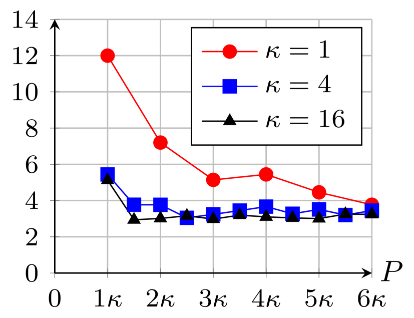
(a) Deterministic sampling

(b) Sobol sampling

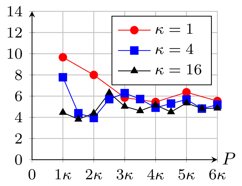
(c) Random sampling

Figure 13: Ratio $\widetilde{M}^{*}(P,\sigma)/N_{P}$ with respect to the truncation parameter $P$ for various types of sampling method and $\sigma=10^{-12}$. The number of EPWs necessary to approximate elements of the space $\mathcal{B}_{P}$ to relative accuracy $\sigma$ seems to scale linearly with the space dimension $N_{P}$.

8.6 Triangular domain

We conclude this section with some numerical results on a triangular geometry. Our purpose is to show that the approximation sets that we constructed also exhibit good approximation properties on other shapes, despite being built following the analysis for the disk.

We consider a triangle $\Omega$ inscribed in the unit disk, with vertices $\mathbf{v}_{1}=(1,0)$, $\mathbf{v}_{2}=(-1,0)$ and $\mathbf{v}_{3}=(\cos(5\pi/8),\sin(5\pi/8))$. The target of the approximation problem is the Helmholtz fundamental solution $\mathbf{x}\mapsto({\imath}/{4})H^{(1)}_{0}(\kappa|\mathbf{x}-\mathbf{s}|)$, for wavenumber $\kappa=16$ and for two different locations $\mathbf{s}\in\mathbb{R}^{2}\setminus\overline{\Omega}$ of the singularity, see Figure 14.

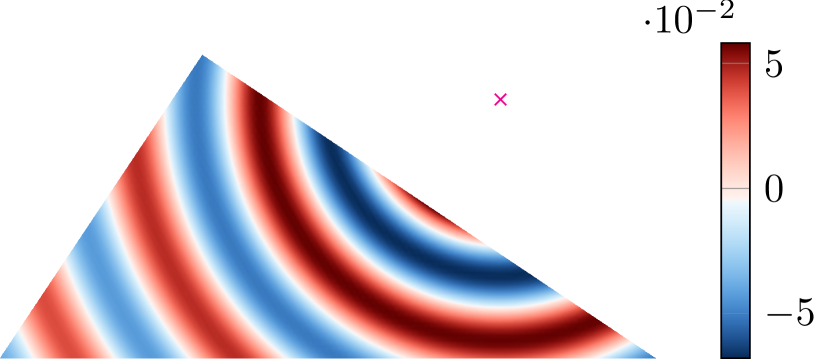
(a) Singularity close to one edge.

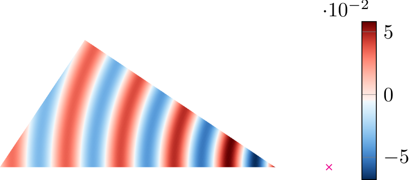
(b) Singularity close to one vertex.

Figure 14: Real part of the fundamental solutions used as target for the approximation problem in the triangle. The magenta cross ${\color[rgb]{1,0,1}\times}$ indicates the position of the singularity $\mathbf{s}$ and is located one wavelength $\lambda=2\pi/\kappa$ away from the boundary of the triangle. Wavenumber $\kappa=16$.

We study the convergence of the approximation by plane waves for increasing size of the approximation set $M$. The approximation is constructed as indicated in Section 3.2–3.3 from Dirichlet data at equispaced points on the boundary of the triangle and by solving the oversampled linear systems using a regularized SVD. The plane waves used in the approximation sets are either propagative, with uniformly spaced angles as described in (4.2), or evanescent, as described in (7.11). The approximation set using EPWs is constructed from sampling the probability density function $\rho_{P}$ defined in (7.7) following a Sobol sequence. For a given size $M$ of the approximation set, the Fourier truncation parameter is computed as $P:=\max\left(\lceil\kappa\rceil,\lfloor M/4\rfloor\right)$, as suggested by Figure 13(b). Finally, the EPWs are re-normalized to have unit $L^{\infty}$ norm on the boundary of the triangle. The latter normalization is the only modification with respect to the sets used for the circular geometry.

The convergence results are presented in Figure 15. When using PPWs, the residual initially decreases rapidly with $M$ but stalls well before reaching machine precision due to the rapidly growing coefficients. In contrast, when using EPWs, the residual converges to machine precision and the size of the coefficients remains moderate when the final accuracy is reached.

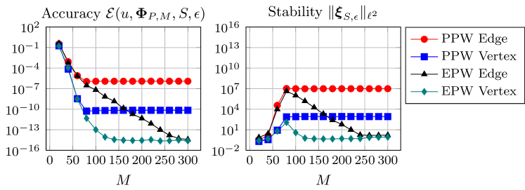
Figure 15: Accuracy $\mathcal{E}$, as defined in (3.15), (left) and stability $\|\boldsymbol{\xi}_{S,\epsilon}\|_{\ell^{2}}$ (right) of the approximation of the fundamental solutions on the triangle $\Omega$ (see Figure 14 for the meaning of the “edge” and “vertex” configurations) by PPWs or EPWs. Wavenumber $\kappa=16$ and regularization parameter $\epsilon=10^{-14}$. The convergence with respect to the size of the approximation set $M$ stalls when using PPWs, due to the need for large coefficients, while EPWs reach machine precision.

We also report in Figure 16 the point-wise absolute error in the bulk of the triangle between the exact solution and the computed approximation, linearly interpolated on a triangular mesh for visualisation purposes. The $L^{\infty}$-norm of the error inside the triangle is of the same order of magnitude as the residual reported in Figure 15. The error with EPWs is of the order of machine precision, whereas the error with PPWs is mainly concentrated on the boundary of the triangle.

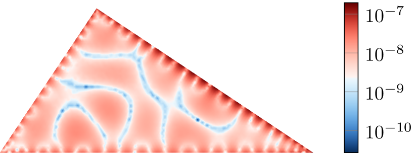
(a) PPW - Edge

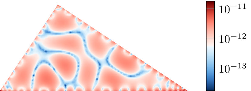
(b) PPW - Vertex

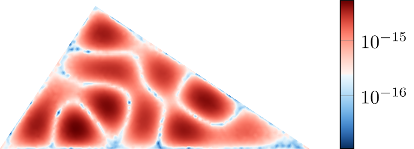
(c) EPW - Edge

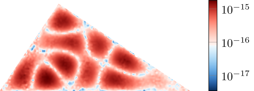
(d) EPW - Vertex

Figure 16: Point-wise error in the triangle between the target of the approximation problem (see Figure 14) and the approximation using propagative (top) and evanescent (bottom) plane waves. The singularity in the solution is either close to the edge (left) or close to the vertex (right). Wavenumber $\kappa=16$ and $M=300$.

These results show the potential of the proposed numerical recipe for Trefftz methods and plane wave approximations. This is even more striking considering that the numerical recipe used to construct the approximations is not tuned for the triangular geometry, with the exception of the re-normalization. Better rules adapted to the underlying geometry might yield even more efficient approximation schemes and are the subject of ongoing investigations.

9 Conclusions

Ill-conditioning is inherent in plane-wave based Trefftz schemes but can be overcome if there exist accurate approximations that are moreover stable, in the sense of having expansions with bounded coefficients. To approximate Helmholtz solutions, PPWs are known to provide accurate approximations. However, the associated expansions are necessarily unstable: the norm of the coefficients blow up for solutions with high-frequency Fourier modes. In contrast, EPWs, which contain high-frequency content, give accurate as well as stable results. To construct stable sets of EPWs, we show numerically that an effective strategy is to sample the parametric domain according to a fully explicit probability measure.

This paper is only the first step towards stable and accurate approximation schemes based on EPWs. A theoretical problem that we have left open is the analysis of the approximation properties of the sets of EPWs constructed using our numerical recipe. Next steps include the extensions to more general geometries, three-dimensional problems (see [19]), time-harmonic Maxwell and elastic wave equations, the application to Trefftz schemes and to sound-field reconstruction algorithms. Preliminary experiments show that the proposed numerical recipe performs well for convex polygons and in Trefftz-Discontinuous Galerkin schemes with several cells, and provides a considerable improvement over standard PPW schemes.

Acknowledgements

The authors are grateful to Albert Cohen, Matthieu Dolbeault and Ralf Hiptmair for helpful discussions, and to Nicola Galante for his careful proofreading. AM and EP acknowledge support from PRIN project “NA–FROM–PDEs” and from MIUR through the “Dipartimenti di Eccellenza” Program (2018–2022) – Dept. of Mathematics, University of Pavia.

Appendix A Proofs of Section 2

Proof of Lemma 2.2.

We only need to prove that the family $\{b_{p}\}_{p\in\mathbb{Z}}$ is orthogonal, which is a consequence of the orthogonality of the complex exponentials $\{\theta\mapsto e^{\imath p\theta}\}_{p\in\mathbb{Z}}$ on the unit circle $\partial B_{1}$. For $p,q\in\mathbb{Z}$, we have

$$(\tilde{b}_{p},\,\tilde{b}_{q})_{L^{2}(B_{1})}=\int_{0}^{1}J_{p}(\kappa r)J_{q}(\kappa r)r\;\mathrm{d}r\int_{0}^{2\pi}e^{\imath(p-q)\theta}\;\mathrm{d}\theta=2\pi\int_{0}^{1}J_{p}^{2}(\kappa r)r\;\mathrm{d}r\;\delta_{pq}.$$ (A.1)

The orthogonality in $H^{1}(B_{1})$ is easily seen from

$$(\nabla\tilde{b}_{p},\,\nabla\tilde{b}_{q})_{L^{2}(B_{1})^{2}}=(\partial_{\mathbf{n}}\tilde{b}_{p},\,\tilde{b}_{q})_{L^{2}(\partial B_{1})}-(\Delta\tilde{b}_{p},\,\tilde{b}_{q})_{L^{2}(B_{1})}=(\partial_{\mathbf{n}}\tilde{b}_{p},\,\tilde{b}_{q})_{L^{2}(\partial B_{1})}+\kappa^{2}(\tilde{b}_{p},\,\tilde{b}_{q})_{L^{2}(B_{1})},$$ (A.2)

where we denoted by $\mathbf{n}$ the outward unit normal vector and

$$(\partial_{\mathbf{n}}\tilde{b}_{p},\,\tilde{b}_{q})_{L^{2}(\partial B_{1})}=\kappa J_{p}^{\prime}(\kappa)J_{q}(\kappa)\int_{0}^{2\pi}e^{\imath(p-q)\theta}\;\mathrm{d}\theta=2\pi\kappa J_{p}^{\prime}(\kappa)J_{p}(\kappa)\delta_{pq}.$$ (A.3)

∎

Proof of Lemma 2.3.

It is straightforward to check that any $b_{p}$, for $p\in\mathbb{Z}$, is solution to the Helmholtz equation (1.1). The continuity of the Helmholtz operator

$$\mathcal{L}\;:\;H^{1}(B_{1})\to H^{-1}(B_{1})=\left(H^{1}_{0}(B_{1})\right)^{*},\ \text{defined by:}$$ (A.4)

$$\langle\mathcal{L}u,\,v\rangle_{H^{-1}\times H^{1}_{0}}:=\left(\nabla u,\,\nabla v\right)_{L^{2}(B_{1})}-\kappa^{2}\left(u,\,v\right)_{L^{2}(B_{1})},\qquad\forall u\in H^{1}(B_{1}),\ v\in H^{1}_{0}(B_{1}),$$

implies that the kernel of $\mathcal{L}$ is a closed subspace of $H^{1}(B_{1})$. From the definition of $\mathcal{B}$ given in (2.2), it follows that

$$\mathcal{B}\subset\ker\mathcal{L}:=\left\{u\in H^{1}(B_{1})\;|\;\mathcal{L}u=0\right\}.$$ (A.5)

Conversely, let $u\in H^{1}(B_{1})$ satisfy (1.1) and set $g:=\partial_{\mathbf{n}}u-\imath\kappa u\in H^{-1/2}(\partial B_{1})$. The Robin trace $g$ can be written

$$g(\theta)=\sum_{p\in\mathbb{Z}}\hat{g}_{p}e^{\imath p\theta},\qquad\forall\theta\in[0,2\pi),\quad\text{with}\quad\sum_{p\in\mathbb{Z}}|\hat{g}_{p}|^{2}(1+p^{2})^{-1/2}<\infty.$$ (A.6)

Let $P\geq 0$, and set $g_{P}(\theta):=\sum_{|p|<P}\hat{g}_{p}e^{\imath p\theta}$, for $\theta\in[0,2\pi)$. Then there exists a unique $u_{P}\in\operatorname{span}\{b_{p}\}_{|p|<P}$, such that $g_{P}=\partial_{\mathbf{n}}u_{P}-\imath\kappa u_{P}$, namely $u_{P}=\sum_{|p|<P}\hat{g}_{p}(\kappa\beta_{p}(J^{\prime}_{p}(\kappa)-\imath J_{p}(\kappa)))^{-1}b_{p}$ (the term $J^{\prime}_{p}(\kappa)-\imath J_{p}(\kappa)$ at the denominator is non-zero because of [31, Eq. (10.21.2)]). The well-posedness [28, Prop. 8.1.3] of the problem: find $v\in H^{1}(B_{1})$ such that

$$-\Delta v-\kappa^{2}v=0,\quad\text{in}\ B_{1},\qquad\text{and}\qquad\partial_{\mathbf{n}}v-\imath\kappa v=h,\quad\text{on}\ \partial B_{1},$$ (A.7)

for $h\in H^{-1/2}(\partial B_{1})$, implies that there exists a constant $C>0$, independent of $P$, such that $\|u-u_{P}\|_{\mathcal{B}}\leq C\|g-g_{P}\|_{H^{-1/2}(\partial B_{1})}$. Letting $P$ tend to infinity, we obtain that $u\in\mathcal{B}$. ∎

Proof of Lemma 2.4.

The explicit expression for $\beta_{p}$ can be deduced by integrating by parts as in the proof of Lemma 2.2. From (A.2), the explicit expression for the boundary term (A.3) and [31, Eq. (10.22.5)],

$$\|\tilde{b}_{p}\|^{2}_{L^{2}(B_{1})}=2\pi\int_{0}^{1}J_{p}^{2}(\kappa r)r\;\mathrm{d}r=\pi\left(J_{p}^{2}(\kappa)-J_{p-1}(\kappa)J_{p+1}(\kappa)\right),$$ (A.8)

we deduce the expression in (2.4). Then the asymptotic behavior is obtained by proving that

$$\begin{aligned} &\|\tilde{b}_{p}\|_{L^{2}(\partial B_{1})}\sim\left({e\kappa}/{2}\right)^{|p|}\;|p|^{-\left(|p|+1/2\right)},\\ &\|\tilde{b}_{p}\|_{L^{2}(B_{1})}\sim 2^{-1/2}\left({e\kappa}/{2}\right)^{|p|}\;|p|^{-\left(|p|+1\right)},\\ &\|\tilde{b}_{p}\|_{\mathcal{B}}\sim\kappa^{-1}\left({e\kappa}/{2}\right)^{|p|}\;|p|^{-|p|},\end{aligned}\qquad\text{as}\ |p|\to+\infty.$$ (A.9)

For any $p\in\mathbb{Z}$, $J_{-p}=(-1)^{p}J_{p}$ from [31, Eq. (10.4.1)]. Therefore, the asymptotic behavior will not depend on the sign of $p$, and we suppose $p>0$ in the following. We start with the trace: from the definition (2.2) of $\tilde{b}_{p}$, $\|\tilde{b}_{p}\|^{2}_{L^{2}(\partial B_{1})}=2\pi J_{p}^{2}(\kappa),$ and from [31, Eq. (10.19.1)], namely

$$J_{\nu}\left(z\right)\sim({2\pi\nu})^{-1/2}({ez}/{2\nu})^{\nu},\qquad\text{as}\ \nu\to+\infty,\qquad z\neq 0,$$ (A.10)

the first result in (A.9) follows. We now consider the $L^{2}(B_{1})$ norm. From (A.8) and (A.10), we get as $p\to+\infty$

$$\|\tilde{b}_{p}\|^{2}_{L^{2}(B_{1})}\sim\frac{1}{2}\left(\frac{e\kappa}{2}\right)^{2p}\;p^{-\left(2p+1\right)}\left[1-\frac{p^{2p+1}}{(p-1)^{p-1/2}(p+1)^{p+3/2}}\right],$$ (A.11)

and it is readily checked that the term inside the square brackets is equivalent to $p^{-1}$ at infinity, so the second result in (A.9) follows. We now consider the $\kappa$-weighted $H^{1}(B_{1})$ norm (2.1). We need to study the asymptotic of the boundary term (A.3). From [31, Eq. (10.6.1)]

$$(\partial_{\mathbf{n}}\tilde{b}_{p},\,\tilde{b}_{p})_{L^{2}(\partial B_{1})}=2\pi\kappa J_{p}^{\prime}(\kappa)J_{p}(\kappa)=\pi\kappa\big{(}J_{p-1}(\kappa)-J_{p+1}(\kappa)\big{)}J_{p}(\kappa).$$ (A.12)

From (A.10), we get as $p\to+\infty$

$$(\partial_{\mathbf{n}}\tilde{b}_{p},\,\tilde{b}_{p})_{L^{2}(\partial B_{1})}\sim\frac{\kappa}{2}\left(\frac{e\kappa}{2}\right)^{2p}\;p^{-\left(2p+1\right)}\left[\frac{2}{e\kappa}\frac{p^{p+1/2}}{(p-1)^{p-1/2}}-\frac{e\kappa}{2}\frac{p^{p+1/2}}{(p+1)^{p+3/2}}\right],$$ (A.13)

and it is readily checked that the first term inside the square brackets is dominant and equivalent to $\frac{2}{\kappa}p$ at infinity. Thus, the dominant term in (A.2) in the limit $p\to\infty$ is the boundary term. ∎

Appendix B Proofs of Section 3

Proof of Proposition 3.2.

The method of proof closely follows that of [2, Th. 3.7]. In particular we first establish a so-called Marcinkiewicz–Zygmund condition, akin to [2, Eq. (3.2)].

The regularity assumption for $u$ and $\boldsymbol{\Phi}_{k}$, which are assumed in $\mathcal{B}\cap C^{0}(\overline{B_{1}})$, allows to have well-defined pointwise evaluations of their image by the Dirichlet trace operator $\gamma$ on the boundary $\partial B_{1}$. Recall that the sampling nodes $\{\mathbf{x}_{s}\}_{s}$ are defined in (3.5). For any $v\in\mathcal{B}\cap C^{0}(\overline{B_{1}})$,

$$\lim_{S\to+\infty}\frac{2\pi}{S}\sum_{s=1}^{S}\left|(\gamma v)(\mathbf{x}_{s})\right|^{2}=\|\gamma v\|_{L^{2}(\partial B_{1})}^{2}.$$ (B.1)

The argument of the limit in the left-hand-side is a Riemann sum approximant of the right-hand-side. A similar argument is developed in [2, Ex. 3.3] (note that $A^{\prime}=B^{\prime}=1$ in the notations of [2]). We will repeatedly use (B.1) in the remainder of the proof.

Let $\boldsymbol{\mu}\in\mathbb{C}^{|\boldsymbol{\Phi}_{k}|}$. From (3.10), we have

$$u-\mathcal{T}_{\boldsymbol{\Phi}_{k}}\boldsymbol{\xi}_{S,\epsilon} =[u-\mathcal{T}_{\boldsymbol{\Phi}_{k}}\boldsymbol{\mu}]+[\mathcal{T}_{\boldsymbol{\Phi}_{k}}A_{S,\epsilon}^{\dagger}A\boldsymbol{\mu}-\mathcal{T}_{\boldsymbol{\Phi}_{k}}\boldsymbol{\xi}_{S,\epsilon}]+[\mathcal{T}_{\boldsymbol{\Phi}_{k}}\boldsymbol{\mu}-\mathcal{T}_{\boldsymbol{\Phi}_{k}}A_{S,\epsilon}^{\dagger}A\boldsymbol{\mu}]$$ (B.2)

$$=[u-\mathcal{T}_{\boldsymbol{\Phi}_{k}}\boldsymbol{\mu}]+\mathcal{T}_{\boldsymbol{\Phi}_{k}}A_{S,\epsilon}^{\dagger}[A\boldsymbol{\mu}-\mathbf{b}]+\mathcal{T}_{\boldsymbol{\Phi}_{k}}[\mathrm{Id}-A_{S,\epsilon}^{\dagger}A]\boldsymbol{\mu}.$$

The proof proceeds by estimating the $L^{2}$ norm of the trace on $\partial B_{1}$ of each term.

The first term appears in the estimate we want to derive, so we examine the second term in (B.2). From (B.1), provided $S$ has been chosen sufficiently large, we can write (picking the constant $2$ on the right-hand-side for simplicity, but any constant $>1$ would work)

$$\|\gamma(\mathcal{T}_{\boldsymbol{\Phi}_{k}}A_{S,\epsilon}^{\dagger}[A\boldsymbol{\mu}-\mathbf{b}])\|_{L^{2}(\partial B_{1})}^{2}\leq 2\frac{2\pi}{S}\sum_{s=1}^{S}|\gamma(\mathcal{T}_{\boldsymbol{\Phi}_{k}}A_{S,\epsilon}^{\dagger}[A\boldsymbol{\mu}-\mathbf{b}])(\mathbf{x}_{s})|^{2}\leq\frac{4\pi}{S}\|AA_{S,\epsilon}^{\dagger}\left[A\boldsymbol{\mu}-\mathbf{b}\right]\|_{\ell^{2}}^{2}.$$ (B.3)

Our choice of regularization (3.9) ensures that $\|AA_{S,\epsilon}^{\dagger}\|\leq 1$, from which we deduce

$$\|\gamma(\mathcal{T}_{\boldsymbol{\Phi}_{k}}A_{S,\epsilon}^{\dagger}[A\boldsymbol{\mu}-\mathbf{b}])\|_{L^{2}(\partial B_{1})}^{2}\leq 2\frac{2\pi}{S}\|A\boldsymbol{\mu}-\mathbf{b}\|_{\ell^{2}}^{2}=2\frac{2\pi}{S}\sum_{s=1}^{S}|\gamma(\mathcal{T}_{\boldsymbol{\Phi}_{k}}\boldsymbol{\mu}-u)(\mathbf{x}_{s})|^{2}.$$ (B.4)

Using once more (B.1), provided $S$ is sufficiently large, we can write (with an additional factor 2)

$$\|\gamma(\mathcal{T}_{\boldsymbol{\Phi}_{k}}A_{S,\epsilon}^{\dagger}[A\boldsymbol{\mu}-\mathbf{b}])\|_{L^{2}(\partial B_{1})}^{2}\leq 4\|\gamma(u-\mathcal{T}_{\boldsymbol{\Phi}_{k}}\boldsymbol{\mu})\|_{L^{2}(\partial B_{1})}^{2}.$$ (B.5)

We now examine the third term in (B.2). Arguing as before, from (B.1), there exists $S$ sufficiently large such that

$$\|\gamma(\mathcal{T}_{\boldsymbol{\Phi}_{k}}[\mathrm{Id}-A_{S,\epsilon}^{\dagger}A]\boldsymbol{\mu})\|_{L^{2}(\partial B_{1})}^{2}\leq 2\frac{2\pi}{S}\sum_{s=1}^{S}|\gamma(\mathcal{T}_{\boldsymbol{\Phi}_{k}}[\mathrm{Id}-A_{S,\epsilon}^{\dagger}A]\boldsymbol{\mu})(\mathbf{x}_{s})|^{2}\leq 2\frac{2\pi}{S}\|A[\mathrm{Id}-A_{S,\epsilon}^{\dagger}A]\boldsymbol{\mu}\|_{\ell^{2}}^{2}.$$ (B.6)

Our choice of regularization (3.9) ensures that $\|A[\mathrm{Id}-A_{S,\epsilon}^{\dagger}A]\|\leq\epsilon\sigma_{\max}$ so that

$$\|\gamma(\mathcal{T}_{\boldsymbol{\Phi}_{k}}[\mathrm{Id}-A_{S,\epsilon}^{\dagger}A]\boldsymbol{\mu})\|_{L^{2}(\partial B_{1})}^{2}\leq 2\frac{2\pi}{S}\epsilon^{2}\sigma_{\max}^{2}\|\boldsymbol{\mu}\|_{\ell^{2}}^{2}.$$ (B.7)

Combining all estimates, (3.11) is readily obtained.

In order to show (3.12), note first that the continuity of the trace operator $\gamma$ from $\mathcal{B}$ to $L^{2}(\partial B_{1})$ allows to write, for any $\boldsymbol{\mu}\in\mathbb{C}^{|\boldsymbol{\Phi}_{k}|}$, $\|\gamma(u-\mathcal{T}_{\boldsymbol{\Phi}_{k}}\boldsymbol{\mu})\|_{L^{2}(\partial B_{1})}\leq\|\gamma\|\;\|u-\mathcal{T}_{\boldsymbol{\Phi}_{k}}\boldsymbol{\mu}\|_{\mathcal{B}}$. It remains to bound the $L^{2}(B_{1})$ norm of $u-\mathcal{T}_{\boldsymbol{\Phi}_{k}}\boldsymbol{\xi}_{S,\epsilon}$, by the $L^{2}(\partial B_{1})$ norm of its trace. Let $\{\hat{e}_{p}\}_{p\in\mathbb{Z}}$ be the coefficients of $e:=u-\mathcal{T}_{\boldsymbol{\Phi}_{k}}\boldsymbol{\xi}_{S,\epsilon}$, in the Hilbert basis $\{b_{p}\}_{p\in\mathbb{Z}}$. From the asymptotics (A.9), we have

$$\|e\|_{\mathcal{B}}^{2}=\sum_{p\in\mathbb{Z}}|\hat{e}_{p}|^{2},\qquad\|e\|_{L^{2}(B_{1})}^{2}=\sum_{p\in\mathbb{Z}}c^{(1)}_{p}\frac{|\hat{e}_{p}|^{2}}{1+p^{2}},\qquad\|e\|_{L^{2}(\partial B_{1})}^{2}=\sum_{p\in\mathbb{Z}}c^{(2)}_{p}\frac{|\hat{e}_{p}|^{2}}{\sqrt{1+p^{2}}},$$ (B.8)

where $\{c^{(1)}_{p}\}_{p\in\mathbb{Z}}$ and $\{c^{(2)}_{p}\}_{p\in\mathbb{Z}}$ are two sequences of positive constants both bounded below and above, and independent of $u-\mathcal{T}_{\boldsymbol{\Phi}_{k}}\boldsymbol{\xi}_{S,\epsilon}$. The sequence $\{c^{(2)}_{p}\}_{p\in\mathbb{Z}}$ is bounded below because $\kappa^{2}$ is not a Dirichlet eigenvalue. We derive (3.12) from this remark and (3.11). ∎

Proof of Corollary 3.3.

Let $\eta>0$ and $u\in\mathcal{B}\cap C^{0}(\overline{B_{1}})$. The stability assumption implies that there exists $\boldsymbol{\Phi}_{k}$ and $\boldsymbol{\mu}\in\mathbb{C}^{|\boldsymbol{\Phi}_{k}|}$ such that

$$\|u-\mathcal{T}_{\boldsymbol{\Phi}_{k}}\boldsymbol{\mu}\|_{\mathcal{B}}\leq\eta\|u\|_{\mathcal{B}}\quad\text{and}\quad\|\boldsymbol{\mu}\|_{\ell^{2}}\leq C_{\mathrm{stb}}|\boldsymbol{\Phi}_{k}|^{s}\|u\|_{\mathcal{B}}.$$ (B.9)

Let $\epsilon\in(0,1]$. Proposition 3.2 implies the existence of $S\in\mathbb{N}$ such that for this particular $\boldsymbol{\mu}$,

$$\|u-\mathcal{T}_{\boldsymbol{\Phi}_{k}}\boldsymbol{\xi}_{S,\epsilon}\|_{L^{2}(B_{1})}\leq C_{\mathrm{err}}\;\Big{(}\|u-\mathcal{T}_{\boldsymbol{\Phi}_{k}}\boldsymbol{\mu}\|_{\mathcal{B}}+\frac{\epsilon\sigma_{\max}}{\sqrt{S}}\|\boldsymbol{\mu}\|_{\ell^{2}}\Big{)}\leq C_{\mathrm{err}}\;\Big{(}\eta+\frac{\epsilon\sigma_{\max}}{\sqrt{S}}C_{\mathrm{stb}}|\boldsymbol{\Phi}_{k}|^{s}\Big{)}\|u\|_{\mathcal{B}}.$$ (B.10)

It remains to choose the free parameters $\eta>0$ and $\epsilon\in(0,1]$ small enough to get the right-hand-side below $\delta$, namely $\eta\leq\frac{\delta}{2C_{\mathrm{err}}}$ and $\epsilon\leq\epsilon_{0}$ with $\epsilon_{0}$ given in (3.14). ∎

References

- [1] Ben Adcock and Daan Huybrechs “Frames and numerical approximation” In SIAM Rev. 61.3, 2019, pp. 443–473 DOI: 10.1137/17M1114697
- [2] Ben Adcock and Daan Huybrechs “Frames and numerical approximation II: Generalized sampling” In J. Fourier Anal. Appl. 26.6, 2020, pp. Paper No. 87\bibrangessep34 DOI: 10.1007/s00041-020-09796-w
- [3] Pedro RS Antunes “A numerical algorithm to reduce ill-conditioning in meshless methods for the Helmholtz equation.” In Numer. Algorithms 79.3, 2018, pp. 879–897
- [4] A.. Barnett “Dissipation in Deforming Chaotic Billiards”, 2000
- [5] A.. Barnett and T. Betcke “Stability and convergence of the method of fundamental solutions for Helmholtz problems on analytic domains” In J. Comput. Phys. 227.14, 2008, pp. 7003–7026 DOI: 10.1016/j.jcp.2008.04.008
- [6] Hélène Barucq, Abderrahmane Bendali, Julien Diaz and Sébastien Tordeux “Local strategies for improving the conditioning of the plane-wave ultra-weak variational formulation” In J. Comput. Phys. 441, 2021, pp. Paper No. 110449\bibrangessep18 DOI: 10.1016/j.jcp.2021.110449
- [7] Paul Bratley and Bennett L Fox “Algorithm 659: Implementing Sobol’s quasirandom sequence generator” In ACM Trans. Math. Software 14.1 ACM New York, NY, USA, 1988, pp. 88–100
- [8] Pablo D. Brubeck, Yuji Nakatsukasa and Lloyd N. Trefethen “Vandermonde with Arnoldi” In SIAM Rev. 63.2, 2021, pp. 405–415
- [9] Olivier Cessenat and Bruno Despres “Application of an ultra weak variational formulation of elliptic PDEs to the two-dimensional Helmholtz problem” In SIAM J. Numer. Anal. 35.1, 1998, pp. 255–299 DOI: 10.1137/S0036142995285873
- [10] Stéphanie Chaillat and Francis Collino “A wideband fast multipole method for the Helmholtz kernel: theoretical developments” In Comput. Math. Appl. 70.4, 2015, pp. 660–678 DOI: 10.1016/j.camwa.2015.05.019
- [11] Gilles Chardon, Albert Cohen and Laurent Daudet “Sampling and reconstruction of solutions to the Helmholtz equation” In Sampl. Theory Signal Image Process. 13.1, 2014, pp. 67–89
- [12] Ole Christensen “An introduction to frames and Riesz bases”, Applied and Numerical Harmonic Analysis Birkhäuser/Springer, [Cham], 2016, pp. xxv+704 DOI: 10.1007/978-3-319-25613-9
- [13] Albert Cohen and Giovanni Migliorati “Optimal weighted least-squares methods” In SMAI J. Comput. Math. 3, 2017, pp. 181–203 DOI: 10.5802/smai-jcm.24
- [14] David Colton and Peter Monk “A novel method for solving the inverse scattering problem for time-harmonic acoustic waves in the resonance region” In SIAM J. Appl. Math. 45.6, 1985, pp. 1039–1053 DOI: 10.1137/0145064
- [15] Scott Congreve, Joscha Gedicke and Ilaria Perugia “Numerical investigation of the conditioning for plane wave discontinuous Galerkin methods” In European Conference on Numerical Mathematics and Advanced Applications, 2017, pp. 493–500 Springer
- [16] D.Colton and R.Kress “Inverse acoustic and electromagnetic scattering theory. 3rd ed.” In Appl. Math. Sci. 93 New York, Springer, 2013, pp. xiv + 405
- [17] Elke Deckers et al. “The wave based method: an overview of 15 years of research” In Wave Motion 51.4, 2014, pp. 550–565 DOI: 10.1016/j.wavemoti.2013.12.003
- [18] Daniel Freeman and Darrin Speegle “The discretization problem for continuous frames” In Adv. Math. 345, 2019, pp. 784–813 DOI: 10.1016/j.aim.2019.01.006
- [19] Nicola Galante “Evanescent Plane Wave Approximation of Helmholtz Solutions in Spherical Domains” Master Thesis, Università di Pavia, arXiv:2305.02175, 2023 arXiv:2305.02175 [math.NA]
- [20] Manuel Hahmann, Samuel A Verburg and Efren Fernandez-Grande “Spatial reconstruction of sound fields using local and data-driven functions” In J. Acoust. Soc. Am. 150.6 Acoustical Society of America, 2021, pp. 4417–4428
- [21] Jerrad Hampton and Alireza Doostan “Coherence motivated sampling and convergence analysis of least squares polynomial Chaos regression” In Comput. Methods Appl. Mech. Engrg. 290, 2015, pp. 73–97 DOI: 10.1016/j.cma.2015.02.006
- [22] Ralf Hiptmair, Andrea Moiola and Ilaria Perugia “A survey of Trefftz methods for the Helmholtz equation” In Building bridges: connections and challenges in modern approaches to numerical partial differential equations 114, Lect. Notes Comput. Sci. Eng. Springer, [Cham], 2016, pp. 237–278
- [23] T. Huttunen, P. Gamallo and R.. Astley “Comparison of two wave element methods for the Helmholtz problem” In Comm. Numer. Methods Engrg. 25.1, 2009, pp. 35–52 DOI: 10.1002/cnm.1102
- [24] Daan Huybrechs and Anda-Elena Olteanu “An oversampled collocation approach of the wave based method for Helmholtz problems” In Wave Motion 87, 2019, pp. 92–105 DOI: 10.1016/j.wavemoti.2018.06.001
- [25] Wenyu Jin and W Bastiaan Kleijn “Theory and design of multizone soundfield reproduction using sparse methods” In IEEE Trans. Audio Speech Lang. Process 23.12 IEEE, 2015, pp. 2343–2355
- [26] Stephen Joe and Frances Y. Kuo “Remark on Algorithm 659: implementing Sobol’s quasirandom sequence generator” In ACM Trans. Math. Software 29.1, 2003, pp. 49–57 DOI: 10.1145/641876.641879
- [27] T. Luostari, T. Huttunen and P. Monk “Improvements for the ultra weak variational formulation” In Internat. J. Numer. Methods Engrg. 94.6, 2013, pp. 598–624 DOI: 10.1002/nme.4469
- [28] Jens Markus Melenk “On generalized finite element methods”, 1995
- [29] Giovanni Migliorati and Fabio Nobile “Stable high-order randomized cubature formulae in arbitrary dimension” In J. Approx. Theory 275, 2022, pp. Paper No. 105706\bibrangessep30 DOI: 10.1016/j.jat.2022.105706
- [30] A. Moiola, R. Hiptmair and I. Perugia “Plane wave approximation of homogeneous Helmholtz solutions” In Z. Angew. Math. Phys. 62.5, 2011, pp. 809–837 DOI: 10.1007/s00033-011-0147-y
- [31] “NIST Digital Library of Mathematical Functions” F. W. J. Olver, A. B. Olde Daalhuis, D. W. Lozier, B. I. Schneider, R. F. Boisvert, C. W. Clark, B. R. Miller, B. V. Saunders, H. S. Cohl, and M. A. McClain, eds., http://dlmf.nist.gov/, Release 1.1.1 of 2021-03-15 URL: http://dlmf.nist.gov/
- [32] Vern I. Paulsen and Mrinal Raghupathi “An introduction to the theory of reproducing kernel Hilbert spaces” 152, Cambridge Studies in Advanced Mathematics Cambridge University Press, Cambridge, 2016, pp. x+182 DOI: 10.1017/CBO9781316219232
- [33] E. Perrey-Debain “Plane wave decomposition in the unit disc: convergence estimates and computational aspects” In J. Comput. Appl. Math. 193.1, 2006, pp. 140–156 DOI: 10.1016/j.cam.2005.05.027
- [34] Samuel A Verburg and Efren Fernandez-Grande “Reconstruction of the sound field in a room using compressive sensing” In J. Acoust. Soc. Am. 143.6 Acoustical Society of America, 2018, pp. 3770–3779
- [35] Norbert Weck “Approximation by Herglotz wave functions” In Math. Methods Appl. Sci. 27.2, 2004, pp. 155–162 DOI: 10.1002/mma.448