InterpretTime: a new approach for the systematic evaluation of neural-network interpretability in time series classification

Abstract

We present a novel approach to evaluate the performance of interpretability methods for time series classification, and propose a new strategy to assess the similarity between domain experts and machine data interpretation. The novel approach leverages a new family of synthetic datasets and introduces new interpretability evaluation metrics. The approach addresses several common issues encountered in the literature, and clearly depicts how well an interpretability method is capturing neural network’s data usage, providing a systematic interpretability evaluation framework. The new methodology highlights the superiority of Shapley Value Sampling and Integrated Gradients for interpretability in time-series classification tasks.

1 Introduction

Time series, sequences of indexed data that follow a specific time order, are ubiquitous. They can describe physical systems [1], such as the state of the atmosphere and its evolution, social and economic systems [2], such as the financial market, and biological systems [3], such as the heart and the brain via ECG and EEG signals, respectively. Availability of this type of data is increasing, and so is the need for automated analysis tools capable of extracting interpretable and actionable knowledge from them. To this end, artificial intelligence (AI) technologies, and neural networks in particular, are opening the path towards highly-accurate predictive tools for time-series regression [4] and classification [5] learning tasks. Yet, interpretability of the results produced by these tools is still lacking, undermining their more widespread adoption in critical sectors. To this end, a key issue is the lack of a systematic and accurate evaluation methodology for interpretability methods. This prevents practitioners to adopt the most suitable and accurate interpretability method for the task at hand, aspect that is now strongly demanded in several applications. The lack of a systematic and accurate interpretability evaluation framework is the gap we aim to fill in this work.

Different definitions of what it means for a neural-network model to be interpretable have been formulated. Most of these definitions can be summarised under two categories: transparency and post-hoc explanation [6]. Transparency refers to how a model and its individual constituents work. Post-hoc explanation refers to how a trained model makes predictions and uses the input features it is given. In this work, we consider post-hoc explanation applied to time series classification, because it is seen as the key to meet recent regulatory requirements [7] and translate current research efforts into real-world applications, especially in high risk areas, such as healthcare [8]. Post-hoc explanation methods assign a relevance score to each feature of a sample reflecting its importance to the model for the classification task being performed. The ability to express the specific features used by a neural network to classify a given sample can help humans assess the reliability of the classification produced and allows comparing the model’s predictions with existing knowledge. It also provides a way to understand possible model’s biases which could lead to the failure of the model in a real-world setting.

A range of methods to provide post-hoc explanation have been developed in the past few years to interpret classification results. These are mainly focused on natural language processing (NLP) and image classification tasks. More recently, with the growing interest for neural-network interpretability, leading actors in the machine learning community built a range of post-hoc interpretability methods. As part of this effort, Facebook recently released the Captum library to group a large number of interpretability methods under a single developmental framework [9]. While these initiatives allow researchers to use the different interpretability methods more easily, they do not provide a systematic and comprehensive evaluation of those methods on data with different characteristics and across neural-network architectures. A systematic methodology that provides the accurate evaluation of these methods is of paramount importance to allow their wider adoption, and measure how trustable the results they provide are.

The evaluation of interpretability methods was initially based on a heuristic approach, where the relevance attributed to the different features was compared to the expectation of an observer for common image classification tasks [10], or of a domain expert for more complex tasks [11, 12]. However, these works had a common pitfall: they assumed the representation of a task learned by a neural network should use the same features as a human expert. The community later moved towards the idea that the evaluation should be independent of human judgement [13]. This paradigm shift was supported by the evidence that certain saliency methods, while looking attractive to human experts, produced results independent of the model they aimed to explain, thereby failing the interpretability task [14]. More recent evaluations were performed by occluding (also referred to as corrupting) the most relevant features identified and comparing the drop in score observed between model’s predictions on the initial and modified samples [15]. This evaluation method was later questioned, as corrupting the images changes the distribution of the sample’s values and therefore the observed drop in score might be caused by this shift in distribution rather than actual information being removed [16]. To address this issue, an approach named ROAR was proposed [16], where important pixels are removed both in the train and test set. The model is then retrained on the corrupted (i.e., occluded) samples, with the drop in score being retained on this newly trained model. This method has the benefit of maintaining a similar distribution across the train and test set. Yet, we argue that it does not necessarily explain which features the initial network used to make its prediction. It rather highlights the properties of the dataset in regards to its target, such as the redundancy of the information present in the features that are indicative of a given class – limitation that was acknowledged by the authors.

Neural-network interpretability for time-series data was only recently explored. Initial efforts applied some of the interpretability methods introduced for NLP and image classification on univariate time series, and evaluated the drop in score obtained by corrupting the most relevant parts of the signal [17]. An evaluation of some interpretability methods was recently proposed [18], with a dataset designed to address the issue of retaining equal distribution between the initial and the occluded dataset. A possible drawback of the proposed dataset is that static properties of the samples, such as the mean, can be used by the neural network to classify a sample. Hence, this task might not reflect the complexity of “real-world" time-series classification tasks, where time dependencies usually play the discriminative role. In addition, the paper lacks a robust evaluation of the different methods independent of human judgement as it is expected that the model uses all the redundant information provided in the dataset.

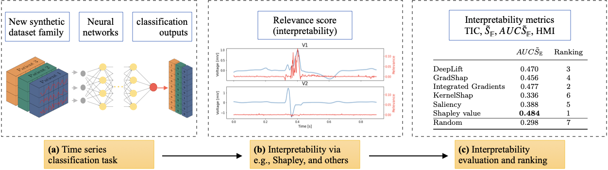
Figure 1: Conceptual interpretability workflow proposed

In this work, we address the several issues plaguing existing interpretability evaluation studies, providing a new accurate approach for the model-agnostic evaluation and benchmarking of interpretability methods for time series classification. In figure 1, we depict the interpretability workflow underlying the new approach (part of the InterpretTime library freely available in Github), where we (a) train different neural network architectures on a new family of synthetic datasets (and ECG datasets), (b) extract the relevance score by using several state-of-the-art interpretability methods available in the literature, (c) evaluate the interpretability methods using the new metrics proposed in this work.

The interpretability methods we considered are six, namely: i) DeepLift [19], ii) GradShap [11], iii) Integrated Gradients [20], iv) KernelShap [11], v) Saliency [21], vi) Shapley Value Sampling (also referred to as Shapley Sampling) [22]. These were chosen to capture a broad range of available interpretability methods, while maintaining the problem computationally tractable for all the models presented. These interpretability methods are applied to three neural-network architectures, namely convolutional (CNN), bidirectional long-short term memory (bi-LSTM), and transformer neural networks. The evaluation of the interpretability methods for time-series classification is carried out on a new family of synthetic datasets as well as on an ECG dataset.

The new family of datasets aims to mimic arbitrary complex multivariate time-series data, and it is based on a nonlinear transformation of chaotic dynamical systems and composed of three datasets. The first synthetic dataset 1, denoted by SD1, simply applies the nonlinear transformation to the dynamical systems, while the second (SD2) and third (SD3) additionally corrupt the time series with different patterns of white noise. Further details are presented in methods 2.1.

The ECG dataset was chosen because the automatic classification of ECGs has seen a growing interest, with recent studies focused on post-hoc neural-network explainability [23, 24], and is of practical interest in “real-world” applications. Additional details on the ECG dataset used here are presented in methods 2.2.

The new approach to interpretability methods’ evaluation is based on novel metrics introduced for time series classification, namely TIC, $S_{\mathbb{E}}$, $AUCS_{\mathbb{E}}$, and HMI. These metrics aim to capture both (i) whether the interpretability method reflects the data representation learned by the model, as well as (ii) how this data representation compares to the one of a domain (human) expert. We call the former relevance identification and attribution, whose key new metrics are TIC, $S_{\mathbb{E}}$, and $AUCS_{\mathbb{E}}$, and are described in methods 1 and 1.1. We call the latter human-machine interpretability, whose key new metric is HMI, and is described in methods 1.2.

In summary, the new synthetic family of datasets, along with the novel interpretability evaluation metrics just outlined address the following key points:

1. The necessity for a robust and quantifiable approach to evaluate and rank interpretability methods’ performance over different neural-network architectures trained for the classification of time series. Our approach addresses the issues found in the literature by providing an evaluation of interpretability methods independent of human judgement [13], using an occluded dataset [15], and without a retrained model [16].

2. The need for a quantitative approach to assess the overlap between a human expert and a neural network in terms of data interpretation. We call this aspect human-machine interpretability.

3. The lack of a synthetic family of datasets with tunable complexity that can be used to assess the performance of interpretability methods, and that is able to reproduce time-series classification tasks of arbitrary complexity.

This paper is organized as follows. In section  2, we present the key results. In section 3 we discuss the results and summarise the main conclusions. In methods, we outline the new approach to interpretability evaluation for time series classification, including the new family of synthetic datasets and the novel metrics.

2 Results

The results are divided by neural-network interpretability methods’ evaluation (section 2.1), and by human-machine interpretability assessment (section 2.2).

All metrics presented in this section are built on the relevance score that an interpretability method provides along the time series. An example for ECG time series is depicted in figure 2, where the red line is the relevance score, while the blue line is the actual time series the neural network is using to make the prediction.

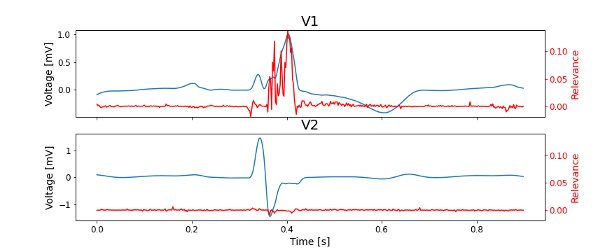
Figure 2: Plot of a sample from the ECG dataset correctly classified with the presence of a RBBB by the Transformer model. The signal of the two selected features (out of 12) is presented in blue along the attributed importance (relevance score) in the classification shown in red. The presented relevance was measured using the Shapley Value Sampling method.

2.1 Interpretability evaluation: relevance identification and attribution

In figure 3, we show the new key metrics for evaluating interpretability methods, for the three different neural networks considered in this work. Each row in the figure corresponds to a given neural network architecture, where the first row corresponds to CNN, the second to bi-LSTM, and the third to transformer. Each column represents a different metric for all the six interpretability methods considered in this work and a baseline which illustrates a random assignment of the relevance.

In particular, the first column shows the normalized drop in score with respect to the neural networks’ expectancy $S_{\mathbb{E}}$ vs. the amount of points deemed important by the interpretability method $\tilde{N}_{\text{r}}$, and consequently removed to compute the drop in score. Both, $S_{\mathbb{E}}$ and $\tilde{N}_{\text{r}}$ are detailed in methods 1.1. These $S_{\mathbb{E}}-\tilde{N}_{\text{r}}$ curves allow evaluating the relevance identification performance of interpretability methods (i.e., the effectiveness of an interpretability method in identifying the relevant portions of the time series that were used by the neural network to make its prediction). The higher the curve the better the interpretability method’s performance.

The second column shows $S_{\mathbb{E}}$ as a function of the time series information content (TIC) index (detailed in methods 1). The latter index measures the amount of information contained in portions of the time series that were used by the neural network to make its prediction. These $S_{\mathbb{E}}-$TIC curves allow a qualitative evaluation of the relevance attribution performance of interpretability methods. Indeed, the difference between the initial classification score and the expectancy of the model’s prediction $\mathbb{E}(S(\mathbf{X}))$ should be linearly proportional to the relevance removed using the TIC index. This theoretical linear trend is depicted in the figure as a dashed line in the plot. The interpretability method closest to this trend has the best relevance attribution performance.

Finally, the third column shows the accuracy of the neural network predictions as a function of $\tilde{N}_{\text{r}}$. The accuracy drop has often been used to evaluate interpretability methods. It is however very dependent on the underlying class distribution of the sample, especially for unbalanced dataset similar to the ECG dataset presented in this paper. Given the latter, $S_{\mathbb{E}}$ was favored as the evaluation metric.

The results presented in figure 3 correspond to the second synthetic dataset, SD2, using an occlusion method (i.e., corruption of the underlying time series) based on normal sampling as described in methods 1.1. Corresponding figures for SD1, and SD3 are reported in extended data figure 1 and 2. Possible biases related to not maintaining i.i.d distribution between the train and test set are addressed by replicating the occlusion of the signals using a permutation of the time steps (as opposed to normal sampling). Figures for all three synthetic datasets using permutation as occlusion method are reported in extended data figure 3,  4 and  5. Results on the ECG dataset can be found in extended data figure 6 and 7.

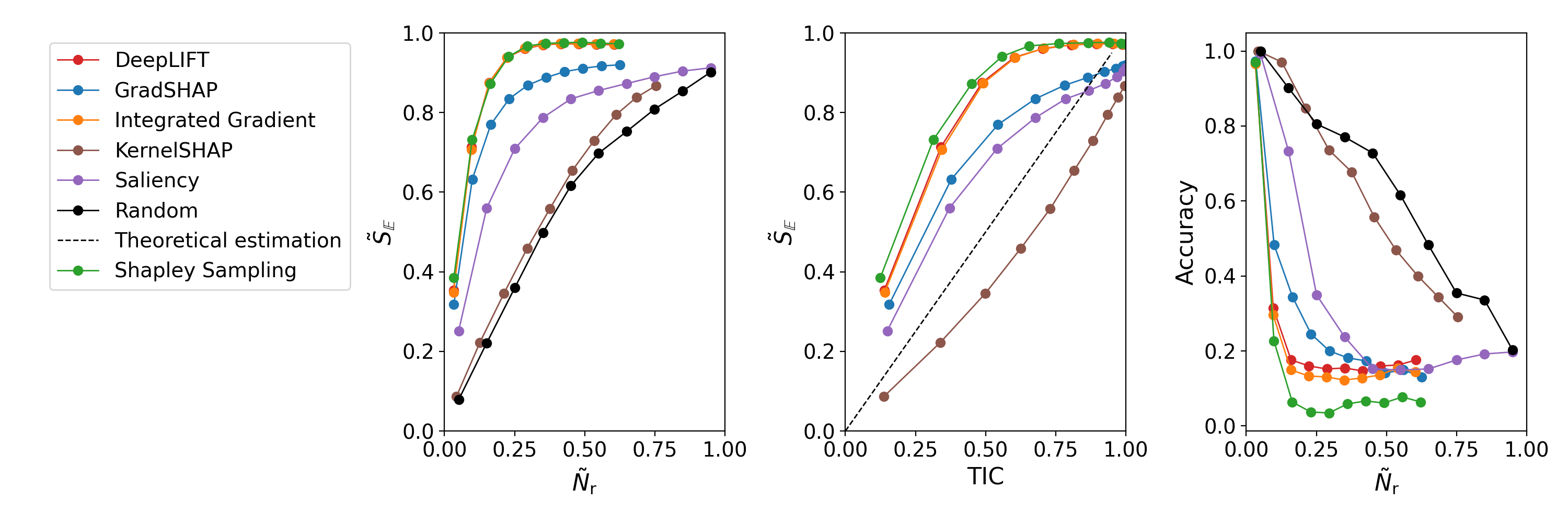
(a) CNN

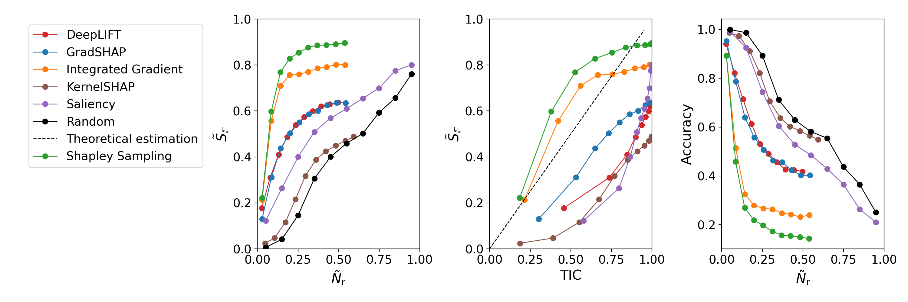
(b) Bi-LSTM

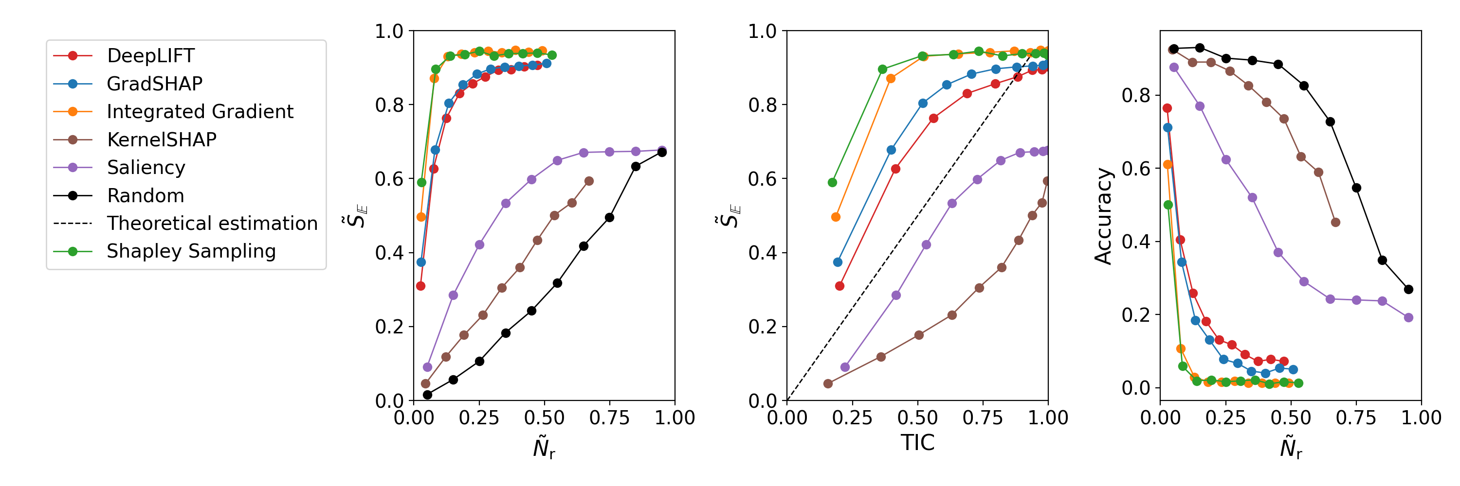
(c) Transformer

Figure 3: Metrics $\tilde{S}_{\mathbb{E}}$ as a function of ratio of points removed $\tilde{N}_{\text{r}}$ (left column) and TIC (middle column), and accuracy as a function of ratio of points removed (right column), for (a) CNN, (b) bi-LSTM, and (c) transformer, using the synthetic dataset 2 (SD2) and normal sampling.

The area under the $\tilde{S}_{\mathbb{E}}-\tilde{N}_{\text{r}}$ curve, namely $AUCS_{\mathbb{E}}$, is used as an indicator of interpretability methods’ performance in identifying the correct portions of the time series that were used by the neural network to make its prediction. Hence, $AUCS_{\mathbb{E}}$ is used to rank the interpretability methods considered in this work. In table 1, we show $AUC\tilde{S}_{\mathbb{E}}$, for the three synthetic datasets introduced in methods 2.1, namely synthetic dataset 1 (SD1), 2 (SD2), and 3 (SD3), when the signal is corrupted with noise sampled from a normal distribution. We also report the ranking of the interpretability methods based on the average $AUC\tilde{S}_{\mathbb{E}}$ across the three datasets, where bold indicates the best performing method (ranking equal to 1). The same results on the ECG dataset are presented in table 2. Results obtained when corrupting the signal by shuffling the time steps are presented in extended data table 1 for the synthetic datasets and extended data table 2 for the ECG dataset, revealing similar results. All models’ hyperparameters and classification scores produced for the trained models are reported in appendix A and B.

Table 1: $AUC\tilde{S}_{\mathbb{E}}$ score for networks trained on the three synthetic datasets SD1, SD2, and SD3, along with the average $AUC\tilde{S}_{\mathbb{E}}$ score across the three synthetic datasets, and the ranking of the interpretability methods based on the average score (bold indicates the best performing interpretability method in terms of $AUC\tilde{S}_{\mathbb{E}}$).

Network	Method	SD1	SD2	SD3	Average	Ranking
CNN	DeepLift	0.877	0.904	0.878	0.886	2
	GradShap	0.816	0.836	0.835	0.829	4
	Integrated Gradients	0.877	0.904	0.879	0.886	2
	KernelShap	0.629	0.610	0.652	0.630	6
	Saliency	0.799	0.755	0.806	0.787	5
	Shapley Sampling	0.883	0.907	0.873	0.888	1
	Random	0.606	0.578	0.634	0.606	7
Bi-LSTM	DeepLift	0.512	0.566	0.607	0.562	5
	GradShap	0.587	0.557	0.598	0.581	4
	Integrated Gradients	0.658	0.738	0.725	0.707	2
	KernelShap	0.437	0.364	0.408	0.403	6
	Saliency	0.651	0.539	0.583	0.591	3
	Shapley Sampling	0.704	0.825	0.749	0.759	1
	Random	0.415	0.388	0.381	0.394	7
Transformer	DeepLift	0.827	0.847	0.774	0.816	4
	GradShap	0.867	0.858	0.780	0.835	3
	Integrated Gradients	0.916	0.916	0.816	0.883	1
	KernelShap	0.430	0.406	0.470	0.435	6
	Saliency	0.463	0.526	0.417	0.469	5
	Shapley Sampling	0.898	0.909	0.830	0.879	2
	Random	0.295	0.314	0.293	0.301	7

Table 2: $AUC\tilde{S}_{\mathbb{E}}$ metric for networks trained on the ECG dataset, along with the ranking of the interpretability methods (bold indicates the best performing interpretability method in terms of $AUC\tilde{S}_{\mathbb{E}}$).

	CNN		Bi-LSTM		Transformer
	$AUC\tilde{S}_{\mathbb{E}}$	Ranking	$AUC\tilde{S}_{\mathbb{E}}$	Ranking	$AUC\tilde{S}_{\mathbb{E}}$	Ranking
DeepLift	0.470	3	0.603	3	0.630	5
GradShap	0.456	4	0.561	4	0.714	3
Integrated Gradients	0.477	2	0.649	2	0.759	2
KernelShap	0.336	6	0.173	7	0.444	6
Saliency	0.388	5	0.332	5	0.659	4
Shapley Sampling	0.484	1	0.652	1	0.802	1
Random	0.298	7	0.182	6	0.437	7

We observe that the relevance identification performance measured by the $AUCS_{\mathbb{E}}-\tilde{N}_{\text{r}}$ curve presents consistent results across the three neural network architectures, with Shapley Sampling and Integrated Gradient showing the best performance (except for CNN on SD3, where DeepLift ranks second together with Integrated Gradients). In terms of relevance attribution, Shapley Sampling and Integrated Gradient overshoot the theoretical linear trend significantly, compared to all other interpretability methods. Yet, none of the methods closely follows the theoretical estimate.

2.2 Human-machine interpretability evaluation

In table 3, we show the human-machine interpretability (HMI) index. This is evaluated on the two synthetic datasets which include time steps where the initial signal has been replaced with non-informative content, SD2 and SD3, respectively. On these two datasets we can attribute an expert score $\omega_{\text{de}}$ equal to 0 on portions of the signal with white noise mimicking the role of a domain expert that knows these portions of the signal are not useful to the classification task. For the rest of the signal $\omega_{\text{de}}$ is set to 1 as by design we know these sections carry information about the target. In bold, we highlight the methods that best match human expert and neural network data interpretation. We observe that these are rather different from the best performing interpretability methods measured in terms of relevance identification. This aspect emphasizes that there is an important distinction between how a human expert might interpret the data as compared to a neural networks.

Table 3: HMI score on the two synthetic datasets with added white noise, SD2, and SD3 (bold indicates best agreement between domain-expert and neural-network data interpretation).

	SD2			SD3
	CNN	Bi-LSTM	Transformer	CNN	Bi-LSTM	Transformer
DeepLift	0.847	0.904	0.802	0.800	0.915	0.699
GradShap	0.864	0.901	0.849	0.853	0.923	0.767
Integrated Gradients	0.847	0.898	0.837	0.789	0.907	0.706
KernelShap	0.803	0.804	0.802	0.609	0.611	0.607
Saliency	0.732	0.916	0.800	0.720	0.930	0.681
Shapley Sampling	0.861	0.886	0.840	0.832	0.914	0.722

The HMI index shown in table 3 opens the opportunity to measure in practical scenarios how human domain experts (e.g., cardiologists in the case of ECG time series classification of hearth disease) interpret data compared to AI solutions. This point is of crucial importance given recent regulatory requirements for the use of AI technologies in critical sectors.

3 Discussion and conclusion

The results presented in section 2 show how the new interpretability metrics are able to correctly assess whether an interpretability method is able to pinpoint the relevant parts of the time series that were actually used by the neural network to make its predictions. In particular, $AUC\tilde{S}_{\mathbb{E}}$ allows quantifying the relevance identification performance of an interpretability method, and is used to rank the methods considered. The $\tilde{S}_{\mathbb{E}}-\text{TIC}$ curves allow a qualitative understanding of the relevance attribution performance. Overall, these two metrics together provide a systematic way of assessing the performance of different interpretability methods, and overcome the several issues highlighted in the existing literature, thereby providing an accurate benchmarking framework for time series classification interpretability.

More specifically, the results shown in tables 1, and 2 highlight an advantage of the Shapley Value Sampling and Integrated Gradients methods across both the synthetic and ECG datasets. This advantage is retained both when corrupting the signal with white noise as well as when permuting the time steps (extended data table 1 and 2). This invariance to corruption methods also address a key issue found in the literature. The drop in performance of an interpretability method has been associated to a shift in terms of distribution between the initial and the corrupted dataset. In our analysis, we show that a larger drop in score is systematically observed both when permuting and when corrupting the most relevant time steps (identified by the interpretability method) as compared to permuting or corrupting a random selection of time steps.

We also note that the Shapley Value Sampling method was the most computing intensive among the methods tested as part of this research. In this regards, the Integrated Gradients can offer a good compromise given its performance across all models and datasets tested given its shorter running time. For the two interpretability methods above, our analysis shows that the most important time steps for a neural network to classify a sample are correctly grasped. However, we observe a discrepancy between the theoretical estimate and the actual curves produced by the different interpretability methods (middle column in figure 3). This indicates that the relevance attributed to each time step does not reflect the relative importance of this time step in the classification task. Instead the attributed relevance acts more as a ranking of the most important time steps among themselves. For example, a point with a relevance of 0.1 for a total classification score of 1 might not necessarily account for 10% of the final prediction but will be more important than a point with a relevance equal to 0.05.

A limitation of the designed methodology is the assumption that time steps are independent and hence their relevance can be estimated separately by occluding the time steps of interest. This assumption does not hold for neural networks which learn dependencies across time steps. This limitation is however taken into account by occluding the quantile of the most relevant time steps. By occluding the most important time steps together and not separately, the most important dependencies are to be captured. Further post processing of the relevance extracted with the interpretability methods should be developed to highlight these dependencies across time steps as well as across features.

Along with the ranking of interpretability methods performance, we introduced the HMI score. This provides a way of assessing whether domain experts and neural networks agree on the time series data interpretation, aspect that to the authors’ knowledge has not been formalized before. The results presented on the synthetic family of datasets, table 3, shows that the interpretability method that best match the intuition of an “expert" do not reflect the interpretability method which achieved the highest $AUC\tilde{S}_{\mathbb{E}}$. This difference between the two metrics reinforces the idea that while it might be of interest to compare the important part of a time series for a given task between a trained model and an expert, it should not be used to assess the performance of an interpretability method.

A key-enabler to achieve the aforementioned results is the novel family of synthetic datasets based on chaotic dynamical systems. This addresses several drawbacks present in existing literature and forces the neural network to learning time dependencies as opposed to learning static information. As part of the presented research, it was shown that the best interpretability methods on the synthetic dataset were also performing best on the ECG dataset emphasising how the designed dataset acts as a good proxy for “real-world" classification task and as such might be used for a range of different research objectives.

Finally, the interpretability computed on the ECG dataset shows how such information might be useful in practical healthcare applications. The relevance presented in figure 2 shows that the most important lead for the model to classify an ECG with the presence of a specific cardiac disease called a right bundle branch block (RBBB) is the lead V1 which is also a diagnostic criteria for cardiologists [25]. Of great interest, the interpretability method is also able to show that the trained model almost entirely rely on this lead to predict a RBBB when there exist other diagnostic criteria for this disease. This type of analysis provides practical insights to understand how trained models will perform in an applied setting, and may help identifying possible biases and potential corrective actions.

Methods

1 Novel approach to interpretability evaluation

The time-series classification task considered in this paper can be formalized as follows. Given a trained neural-network model $\mathcal{N}$, we aim to map a set of features $\mathbf{X}\in\mathbb{R}^{M\times T}$ to a labelled target $\text{C}\in\mathbb{N}^{N_{c}}$, for each sample $i$ contained in a given dataset $\mathcal{D}_{i}=[\mathbf{X},\text{C}]_{i}\;\;\text{for}\;i=1,\dots,N$, where $M$ is the number of features, $T$ is the number of ordered elements per feature, $N_{c}$ is the number of labels, and $N$ is the total number of samples available. Typically, this is achieved by a score $S(\mathbf{X}_{i})$ that the trained neural network $\mathcal{N}$ provides, and that is then used as an input to a softmax layer to output the probability of sample $i$ to belong to a given class C $\in\mathbb{N}^{N_{c}}$.

To assess quantitatively time-series interpretability methods, we developed novel metrics or indices which encompass two key areas:

1. evaluate how closely an interpretability method reflects the representation learned by the model of interest, and

2. how the learned representations compares to the one an expert would use to approach the classification task.

While these two points have often been interchanged to evaluate interpretability methods, we reassert the importance to distinguish them. Hence, we developed independent metrics to evaluate them separately.

The new metrics are built on the relevance score that an interpretability method provides along the time series. The relevance score can be positive or negative (except for some interpretability methods, where it is only positive – see e.g., the saliency method [21]). A positive relevance score means that the neural network is using that portion of the time series to make its prediction. A negative relevance score indicates that the neural network sees the portion of the time series as going against its prediction. As we are interested in how the network is using data to making its predictions, we use the positive relevance score to build the new metrics.

In this work, we considered six interpretability methods: i) DeepLift [19], ii) GradShap [11], iii) Integrated Gradients [20], iv) KernelShap [11], v) Saliency [21], vi) Shapley Value Sampling [22]. These methods were chosen to capture a broad range of available interpretability methods, while maintaining the problem computationally tractable for all the models presented. The implementation of the interpretability methods leveraged those provided in the Captum library [9]. The objective is to evaluate each of the methods above in terms of their performance as well as assess them in terms of human-machine data interpretation.

Central to the analysis of the relevance distribution, we define the time information content (TIC) index as:

$$\text{TIC}(q)=\frac{\int_{\tau}\mathcal{I}^{+}_{q}(q)\text{d}\tau}{\int_{t}\mathcal{I}^{+}\text{d}t+\epsilon}$$ (1)

where $\mathcal{I}^{+}_{q}$ is the set of points with positive relevance above a relevance quantile $q$, $\tau=t\in\mathcal{I}^{+}_{q}$ and $\epsilon$ is a small number that prevents the ratio to diverge to infinity. The TIC index reflects the ratio of the relevance attributed to the set of points $\mathcal{I}^{+}_{q}$ to the total positive relevance $\mathcal{I}^{+}$, integrated over the time series. In the rest of the study, TIC is calculated for each quantile within the following set: $\mathcal{Q}=\{0.05,0.15,0.25,\ldots,0.95\}$. The TIC constitutes a key index for both the ranking of interpretability methods’ performance as well as for human-machine interpretability evaluation described next.

1.1 Relevance identification and attribution

For assessing interpretability methods’ performance, we need to tackle two aspects, relevance identification and relevance attribution. We detail these two concepts along the methods developed to measure them next.

Relevance identification. The concept behind relevance identification is that interpretability methods should correctly identify and order according to their relevance the set of points used by the model to make its predictions. To verify that this is the case, we occlude the set of points $\mathcal{I}^{+}_{q}$ for each quantile $q$ in the quantile set $\mathcal{Q}$. This results in the modified sample $\mathbf{\bar{X}}_{i}$, where $N_{\mathcal{I}^{+}}$ points along the time series are occluded. Given the discussion provided in section 1 and the comments on maintaining i.i.d distribution across the different datasets, we adopt two different occlusion methods. The first method consists in sampling new values from a normal distribution with mean equal to 0 and standard deviation equal to $\frac{1}{2\sqrt{3}}$ to replace the set of values of interest $\mathcal{I}^{+}_{q}$. This first technique might violate the i.i.d property. The second method randomly shuffles values in $\mathcal{I}^{+}_{q}$, instead of sampling them from a normal distribution. This second technique has the benefit of maintaining a constant distribution between the initial samples and the modified ones. A random baseline is created by occluding a set of $N_{\mathcal{I}^{+}}$ random points to provide a comparison between the interpretability metrics and a random assignment of the relevance. We then run our trained model on the modified sample $\mathbf{\bar{X}}_{i}$ and define the normalised drop in score $\tilde{S}_{\mathbb{E}}$ with respect to the network’s expectancy $\mathbb{E}[S(\mathbf{X})]$, where the network’s expectancy is the score average over the entire dataset. The new metric $\tilde{S}_{\mathbb{E}}$ is defined as:

$$\tilde{S}_{\mathbb{E}}\big{\rvert}_{\mathbf{X}=\mathbf{X}_{i},q}=1-\frac{S(\bar{\mathbf{X}}_{i}(q))-\mathbb{E}[S(\mathbf{X})]}{S(\mathbf{X}_{i})-\mathbb{E}[S(\mathbf{X})]}$$ (2)

Using this newly created metric, it is possible to produce $\tilde{S}_{\mathbb{E}}\;\text{vs.}\;\tilde{N}_{\text{r}}$ curves, where $\tilde{N}_{r}$ is the fraction of points removed with respect to the total number of points $T$ present in the time series, i.e. $\tilde{N}_{\text{r}}(q)=\frac{N_{\mathcal{I}^{+}}(q)}{T}$. These curves allow us to understand the effectiveness of interpretability methods vs. the amount of points flagged by the relevance score, and consequently removed. The number of points flagged is strictly linked to the quantile adopted. As we decrease the quantile, we increase $\tilde{N}_{\text{r}}$.

The overall effectiveness of the interpretability method can be summarised as the area under the $\tilde{S}_{\mathbb{E}}-\tilde{N}_{\text{r}}$ curve described above, and denoted as

$$AUC\tilde{S}_{\mathbb{E}}=\int_{0}^{1}\tilde{S}_{\mathbb{E}}\;\text{d}\tilde{N}_{\text{r}}$$ (3)

where $\tilde{S}_{\mathbb{E}}(\tilde{N}_{\text{r}})$ is extended to pass through the origin and $\tilde{S}_{\mathbb{E}}(1)$ is measured at the smallest quantile of the quantile set $\mathcal{Q}$. The aim is to have a fair comparison across all methods which might attribute different number of points with positive relevance.

Relevance attribution. The idea behind relevance attribution is that relevance should reflect the individual contribution of each time step towards the model predicted score. The local accuracy property states that the sum of the relevance should be equal to the difference between the score and the expectancy of the network $\mathbb{E}[S(\mathbf{X})]$ [11]. Extending this property, the difference between the initial score and the expectancy of the model’s predictions $\mathbb{E}[S(\mathbf{X})]$ should be linearly proportional to the relevance removed using the TIC index.

Given this theoretical approximation, it is possible to evaluate how different interpretability methods over- or under-estimate the role of different time steps in the model’s prediction. Indeed the index $\tilde{S}_{\mathbb{E}}$ should be proportionally linear to the TIC index so that the information ratio (IR) satisfies

$$\text{IR}\big{\rvert}_{\mathbf{X}=\mathbf{X}_{i}}=\frac{\Delta\tilde{S}_{\mathbb{E}}(\mathbf{X}_{i},q)}{\Delta\text{TIC}(\mathbf{X}_{i},q)}\rightarrow\mathbb{E}_{\mathbf{X}}\left[\text{IR}\right]=1$$ (4)

A slope larger than one will indicate the relevance of the points under the quantile of interest was under-estimated while the opposite is true for a slope smaller than one. An example of these curves is depicted in figure 3, in the middle column, where we report the theoretical linear line (dashed), and the $\tilde{S}_{\mathbb{E}}-\text{TIC}$ curves for every interpretability method considered.

1.2 Human-machine interpretability

To quantify how the relevance attributed by the interpretability method follows the expectations of domain experts, the TIC index is modified to include domain-expert weights $\omega_{\text{de}}$ and denoted as human-machine intepretability (HMI) score:

$$\text{HMI}=\frac{\int_{\tau}\omega_{\text{de}}\cdot\mathcal{I}^{+}\text{d}\tau}{\int_{\tau}(\mathcal{I}^{+})\text{d}\tau+\epsilon}\cdot\left[1-\gamma_{p}\right]\quad\text{ where }\gamma_{p}=\text{min}\left(1,\frac{\Delta_{N_{w\mathcal{I}^{+}}}}{N_{\mathcal{I}^{+}}}\right)$$ (5)

where $\Delta_{N_{w\mathcal{I}^{+}}}$ is the difference in terms of number of points with positive relevance between the interpretability method and the human expert, $N_{\mathcal{I}^{+}}$ is the number of points having positive relevance identified by the interpretability method, and $\tau$ is the set of time steps with positive relevance $\mathcal{I}^{+}$. The domain-expert weights $\omega_{\text{de}}$ aim to reflect the importance of the different time steps as seen by a domain expert, and can be either zero or one. A value of 0 means that the associated portion of the time series is not important to make a decision. A value of 1 means that the associated portion of the time series is important. Consequently, HMI produces a perfect interpretability score equal to 1, if $\omega_{\text{de}}$ is equal to 1 only on those portions of the time series that were flagged by the relevance score (i.e., by the machine) as important. In this case, the neural network interpretation of the time series would match exactly the one given by the domain expert. However, in the more general case, the domain expert might also flag other parts of the time series as important (the limit case is the domain expert flagging the entire time series as important). In this case, it is necessary to penalize the parts of the time series non-overlapping with the relevance score produced by the machine. This is achieved by penalising the HMI score by the factor $\gamma_{p}$. The latter is equal to 0, if $\Delta N_{w\mathcal{I}^{+}}=0$ (exact overlapping of human and machine interpretation), and equal to 1 if $\Delta N_{w\mathcal{I}^{+}}=N_{\mathcal{I}^{+}}$. We further observe that the fraction constituting $\gamma_{p}$ could be larger than one. If this is the case, we bound the value to 1, for easier interpretation of the score – i.e., $\text{HMI}=0$ means that there is no overlap between human and machine data interpretation.

2 Datasets

The new interpretability evaluation approach has been applied to two sets of data, namely a new family of synthetic datasets created for this work, and an ECG dataset. The two are described next.

2.1 A new family of synthetic datasets

The new family of datasets envisioned for the interpretability of time series classification is based on five different and well-known chaotic dynamical systems, namely Chua [26], Duffing [27], Lorenz [28], Rikitake [29], and Rössler [30]. Each dynamical system (also referred to as attractor) constitutes a different class (or label) in the classification task, and is composed by three time series characterizing the nonlinear dynamics (composed by three state variables) of the attractor.

Dynamical systems are described by a set of differential equations of the form:

$$\frac{d\mathbf{X}}{dt}=F\left(\mathbf{X}\right)$$ (6)

The equations for each of the five dynamical systems used in this paper are defined below. Each system include a range of parameters which are either fixed or randomly sampled for each attractor from a given interval in order to generate different behaviours . The first system used is the Chua system which aims to replicate an electronic circuit with chaotic behavior [26] and can be formulated as [31]:

$$\frac{dx}{dt} =a\cdot\left(y-x-h\right)$$ (7)

$$\frac{dy}{dt} =x-y-z$$

$$\frac{dz}{dt} =-b\cdot y$$

$$\text{with }h =\nu_{2}\cdot x+0.5\cdot\left(\nu_{1}-\nu_{2}\right)\cdot\left(\lvert x+1\rvert-\lvert x-1\rvert\right)$$

with the following constant, $a=15.6$, $\nu_{1}=-1.143$, $\nu_{2}=-0.714$ and $b$ randomly sampled in the interval $[25,51]$.

The second system is the Duffing oscillator which models a forced oscillator, and whose equations are:

$$\frac{dx}{dt} =y$$ (8)

$$\frac{dy}{dt} =-a\cdot{y}-x^{3}+b\cdot\cos\left(\omega\cdot z\right)$$

$$\frac{dz}{dt} =1$$

with $a=0.1$ and $b$ sample from the interval $[0.1,0.65]$.

Third is the Lorenz system which model atmospheric convection [28] and is defined as:

$$\frac{dx}{dt} =\sigma\cdot\left(y-x\right)$$ (9)

$$\frac{dy}{dt} =x\cdot\left(\rho-z\right)-y$$

$$\frac{dz}{dt} =x\cdot y-\beta\cdot z$$

with $\sigma=10$, $\beta=\nicefrac{{8}}{{3}}$ and $\rho$ sampled in the interval $[28,100]$.

Fourth is the Rikitake system which aims to explain the reversal of the Earth’s magnetic field with the following set of equations [29]:

$$\frac{dx}{dt} =-a\cdot x+y\cdot\left(z+c\right)$$ (10)

$$\frac{dy}{dt} =-b\cdot y+x\cdot\left(z-c\right)$$

$$\frac{dz}{dt} =d\cdot z-x\cdot y$$

with $a$ sampled in the interval $[2,7]$ $b=3$, $c=5$, $d=0.75$.

Fifth is the Rössler system which aims to showcase chaotic behavior with fractal properties [30]. The equations for this system are the following:

$$\frac{dx}{dt} =-\left(y+z\right)$$ (11)

$$\frac{dy}{dt} =x+a\cdot y$$

$$\frac{dz}{dt} =b+z\cdot\left(x-c\right)$$

with $a=0.2$, $b=0.2$ and c sampled from the interval $[4,18]$.

All samples were generated by integrating in time the above systems of equations using the 5th order Runge-Kutta method from the desolver Python package.

Table 4: Ranges from which the initial conditions of the different samples are sampled from for the different attractors

	x	y	z
Chua	$[0.6,0.61]$	$[0.2,0.21]$	$[0.1,0.11]$
Duffing	$[0.6,7.5]$	$[0.2,1.5]$	$[0.1,1.6]$
Lorenz	$[0.6,1.1]$	$[0.2,0.7]$	$[0.1,0.6]$
Rikitake	$[0.6,1.1]$	$[0.2,0.7]$	$[0.1,0.6]$
Rössler	$[0.6,1.6]$	$[0.2,1.2]$	$[0.1,1.1]$

The samples were integrated for 3500 time steps with the first 1000 time steps being discarded and the resulting time series being downsampled by a factor of 10. For each attractor class, 500 samples are generated with initial condition and system parameters drawn from a uniform distribution within a prescribed range (the ranges adopted are defined in table 4). Each sample includes 250 time steps. In order to replicate “real-world” time series, that typically come with data corruption due to e.g., sensors issues or external disturbances, each sample is modified using a nonlinear transformation function of the form:

$$\mathbf{a}+\mathbf{b}\sin{\left(\mathbf{c}\cdot x(t)+\mathbf{d}\right)}$$ (12)

where $\mathbf{a},\mathbf{b},\mathbf{c},\textbf{d}\in\mathbb{R}^{1\times 3}$ are parameters also sampled from a uniform distribution and allow to tune the complexity of the classification task.

To force the neural networks to acquire time-series knowledge as opposed to use static knowledge, we rescaled the three time series associated to each attractor so that the maximum norm over the three quantities is one. The mean was also removed from each of the three quantities. These two steps are the key for preventing static metrics to be discriminative between different attractors (i.e. classes). In addition to these transformed and rescaled attractors, that we refer to as synthetic dataset 1 (SD1), we created two additional datasets with data portions replaced by white noise to form the following dataset family:

1. transformed attractors (synthetic dataset 1, or SD1),

2. transformed attractors where random locations are corrupted with white noise (synthetic dataset 2, or SD2),

3. transformed attractors with first 100 time steps of each feature corrupted with white noise (synthetic dataset 3, or SD3),

The rationale behind choosing chaotic dynamical systems for the new synthetic dataset family lies on the similarity between identifying different dynamics, belonging to different phenomena that are common in “real-world” classification tasks such as ECG and EEG disease identification.

Overall the creation of the new synthetic dataset family, which includes three synthetic datasets, allows evaluating the metrics developed in this work, and produces consistent results in terms of interpretability method ranking as well as human-machine interpretability.

2.2 ECG dataset

To mimic a real-world classification task, we applied the interpretability framework to an ECG dataset. ECG records the electrical activity of the heart and typically produces 12 signals, corresponding to 12 sensors or leads. For this task, a subset of the Classification of 12-lead ECGs: the PhysioNet - Computing in Cardiology Challenge 2020 published under CC Attribution 4.0 License was used. The dataset was narrowed down to the CPSC subset [32] which included 6877 ECGs annotated for 9 cardiovascular diseases. As part of these annotations, it was chosen to classify the ECGs for the presence/absence of a Right Bundle Branch Block (RBBB). The dataset includes 5020 cases showing no sign of a RBBB and 1857 cases annotated as carrying a RBBB. RBBB was found to be associated with higher cardiovascular risks as well as mortality [33].

In order to obtain an average beat, the R-peaks of each ECG are extracted using the BioSPPy library [34]. The beats centred around the R-peaks are then extracted from the ECG by taking 0.35 before and 0.55 seconds after the R-peak. The mean of the extracted beat is then computed to obtain an "average" beat from each ECG. An example of the initial signal along the transformed one used as a feature for the classification task are presented in figure 4 and 5.

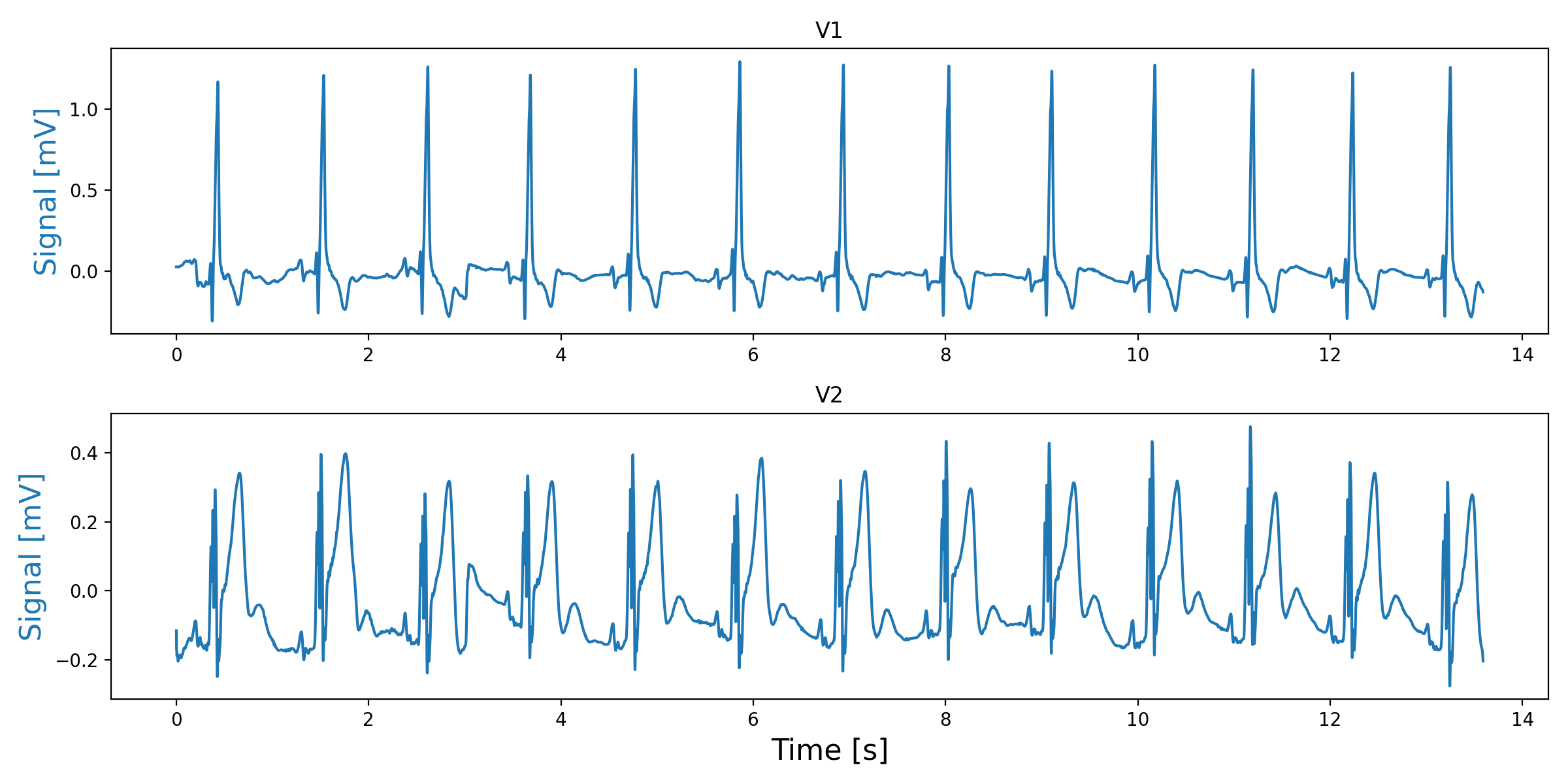
Figure 4: Raw ECG signal for two selected leads from a given sample

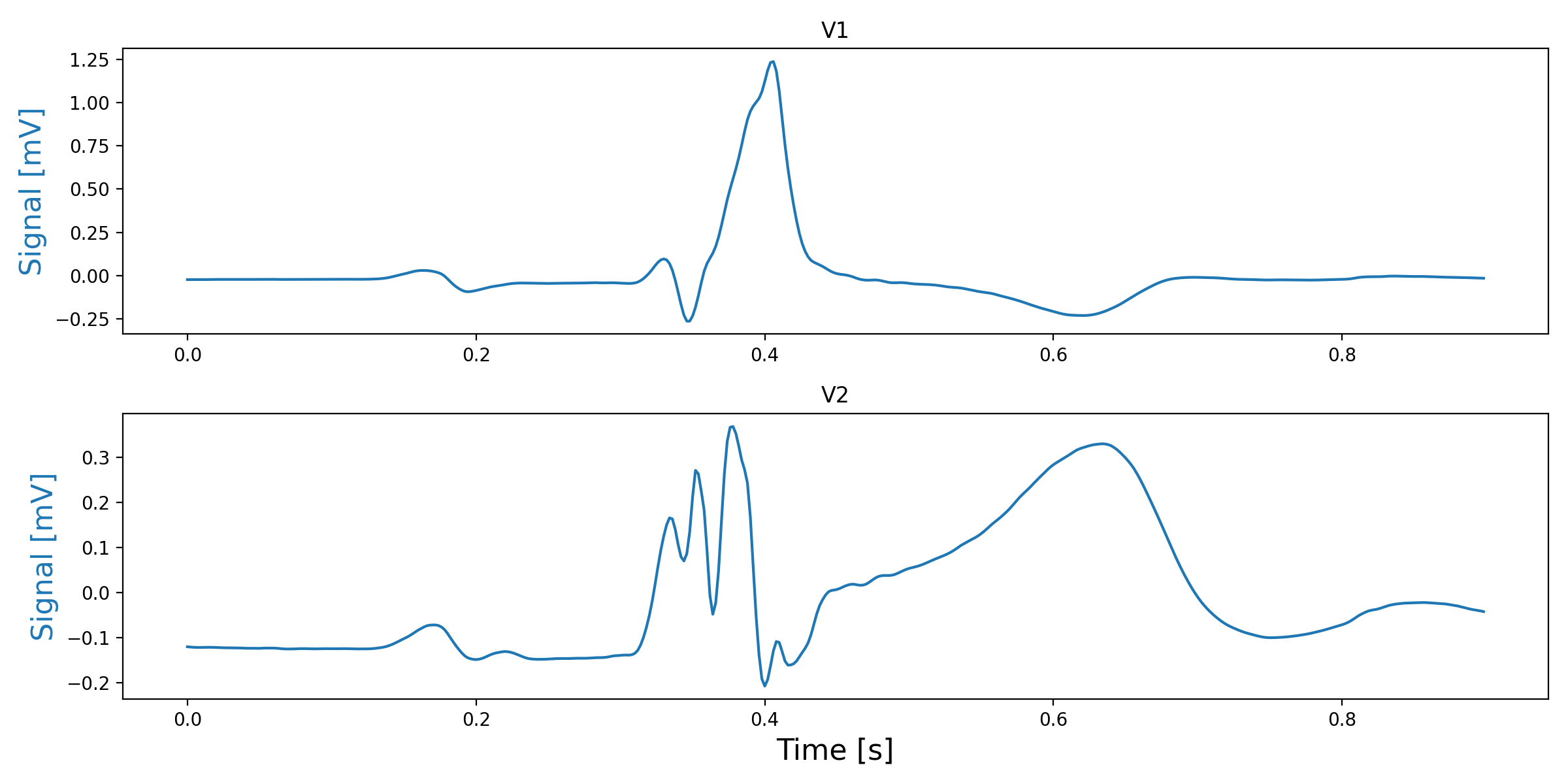
Figure 5: Processed ECG signal for two selected leads from a given sample

Extended data

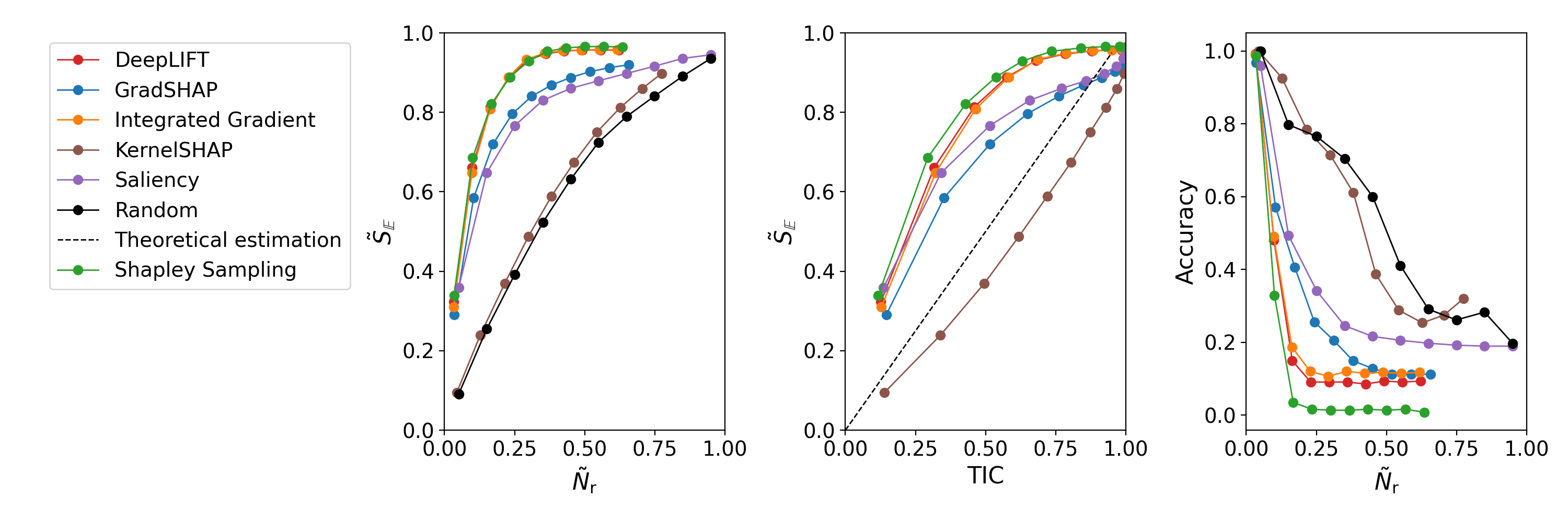
(a) CNN

(b) Bi-LSTM

(c) Transformer

Extended data figure 1: Metrics $\tilde{S}_{\mathbb{E}}$ as a function of ratio of points removed (left column) and TIC (middle column), and accuracy as a function of ratio of points removed (right column), for (a) CNN, (b) bi-LSTM, and (c) transformer, using the synthetic dataset 1 (SD1) and normal sampling.

(a) CNN

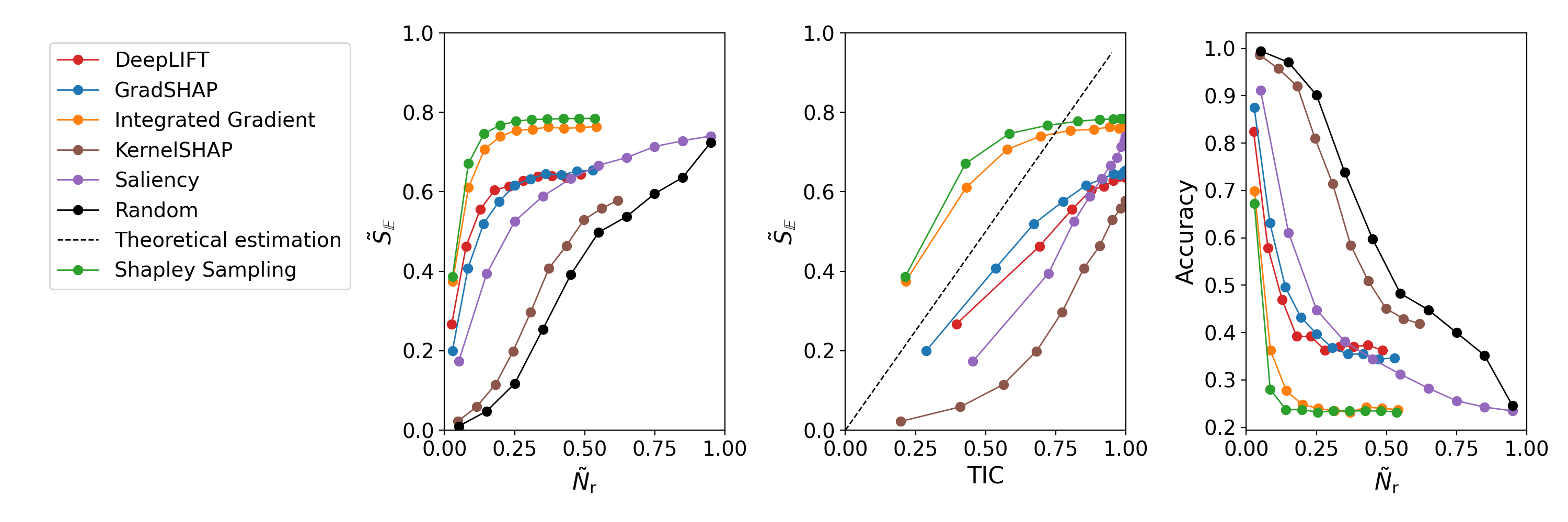
(b) Bi-LSTM

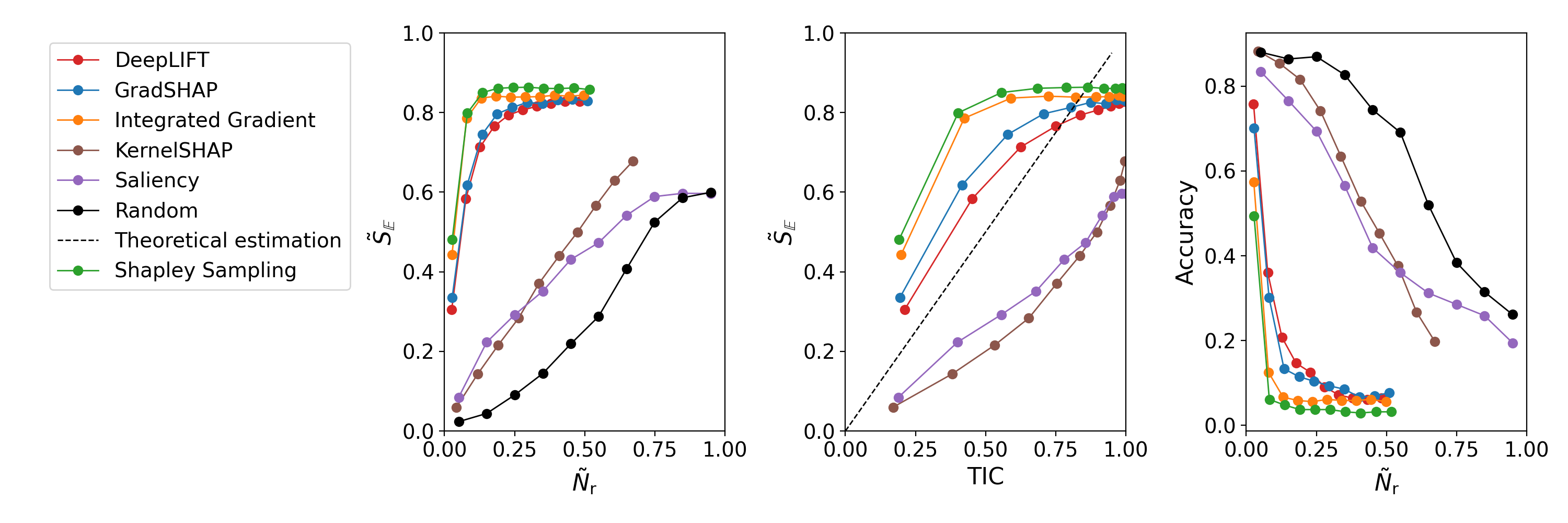
(c) Transformer

Extended data figure 2: Metrics $\tilde{S}_{\mathbb{E}}$ as a function of ratio of points removed (left column) and TIC (middle column), and accuracy as a function of ratio of points removed (right column), for (a) CNN, (b) bi-LSTM, and (c) transformer, using the synthetic dataset 3 (SD3) and normal sampling.

Extended data table 1: Evaluation of the interpretability metrics for networks trained on synthetic datasets with signal corrupted by permuting time steps (bold indicates the best performing interpretability method for each dataset).

Network	Method	SD1	SD2	SD3	Average	Ranking
CNN	DeepLift	0.673	0.661	0.747	0.694	2
	GradShap	0.645	0.639	0.733	0.672	4
	Integrated Gradients	0.671	0.663	0.747	0.694	1
	KernelShap	0.546	0.490	0.629	0.555	6
	Saliency	0.628	0.591	0.718	0.646	5
	Shapley Sampling	0.672	0.666	0.738	0.692	3
	Random	0.535	0.479	0.607	0.540	7
bi-LSTM	DeepLift	0.362	0.289	0.467	0.372	5
	GradShap	0.436	0.381	0.515	0.444	3
	Integrated Gradients	0.438	0.427	0.482	0.449	2
	KernelShap	0.364	0.322	0.406	0.364	6
	Saliency	0.443	0.353	0.498	0.431	4
	Shapley Sampling	0.479	0.459	0.479	0.472	1
	Random	0.345	0.311	0.415	0.357	7
Transformer	DeepLift	0.486	0.477	0.583	0.515	4
	GradShap	0.629	0.556	0.659	0.615	2
	Integrated Gradients	0.615	0.511	0.671	0.599	3
	KernelShap	0.235	0.233	0.342	0.270	5
	Saliency	0.176	0.225	0.282	0.228	6
	Shapley Sampling	0.640	0.553	0.681	0.624	1
	Random	0.150	0.167	0.217	0.178	7

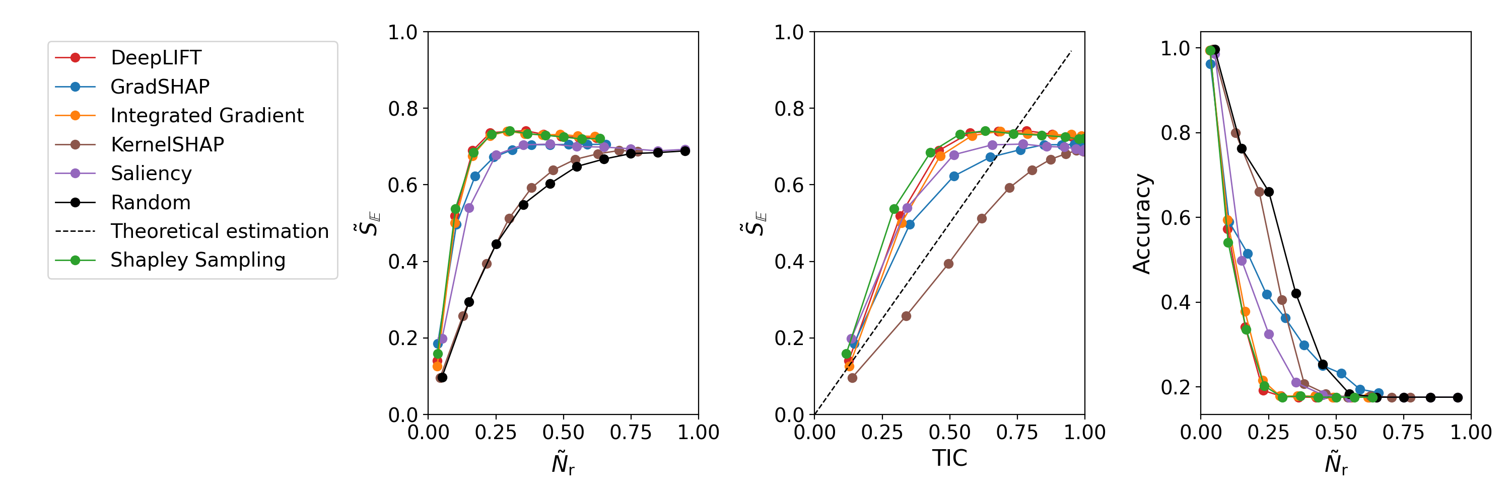
(a) CNN

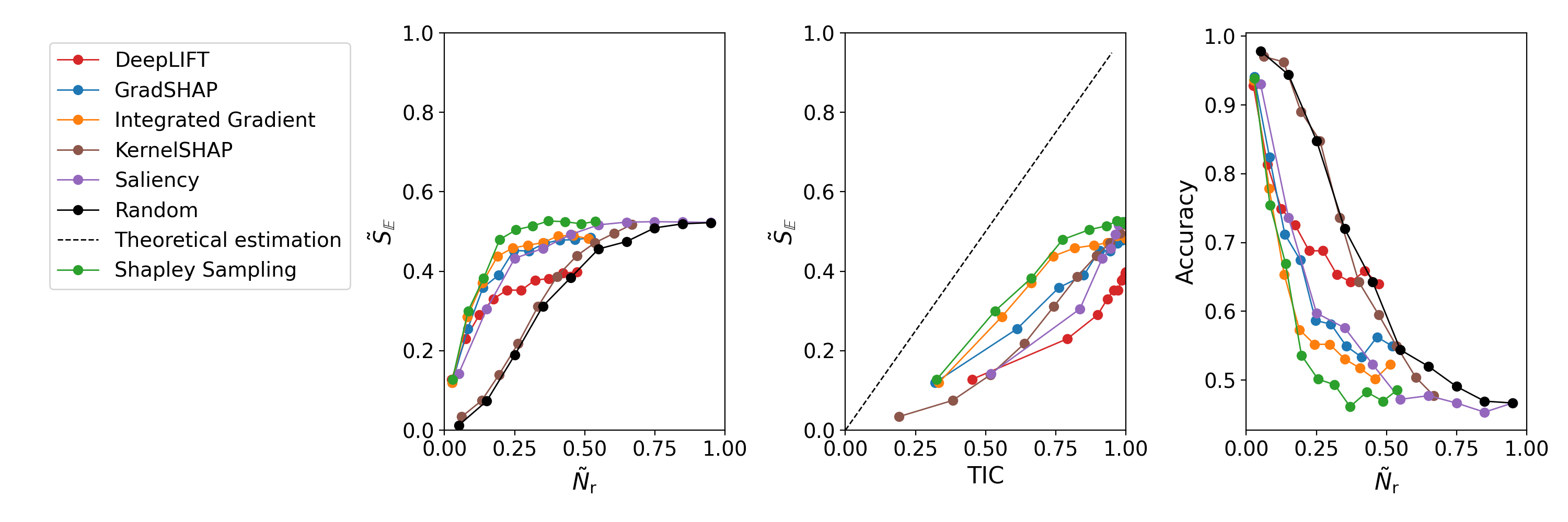
(b) Bi-LSTM

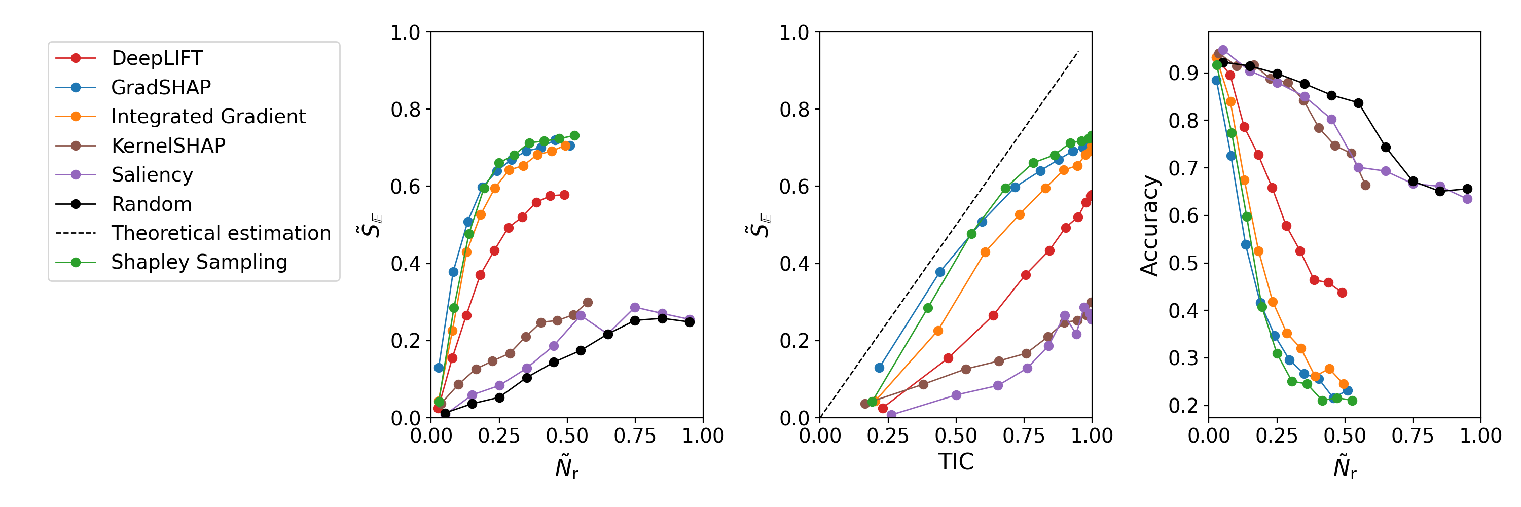
(c) Transformer

Extended data figure 3: Metrics $\tilde{S}_{\mathbb{E}}$ as a function of ratio of points removed (left column) and TIC (middle column), and accuracy as a function of ratio of points removed (right column), for (a) CNN, (b) bi-LSTM, and (c) transformer, using the synthetic dataset 1 (SD1) and permuting the time steps.

(a) CNN

(b) Bi-LSTM

(c) Transformer

Extended data figure 4: Metrics $\tilde{S}_{\mathbb{E}}$ as a function of ratio of points removed (left column) and TIC (middle column), and accuracy as a function of ratio of points removed (right column), for (a) CNN, (b) bi-LSTM, and (c) transformer, using the synthetic dataset 2 (SD2) and permuting the time steps.

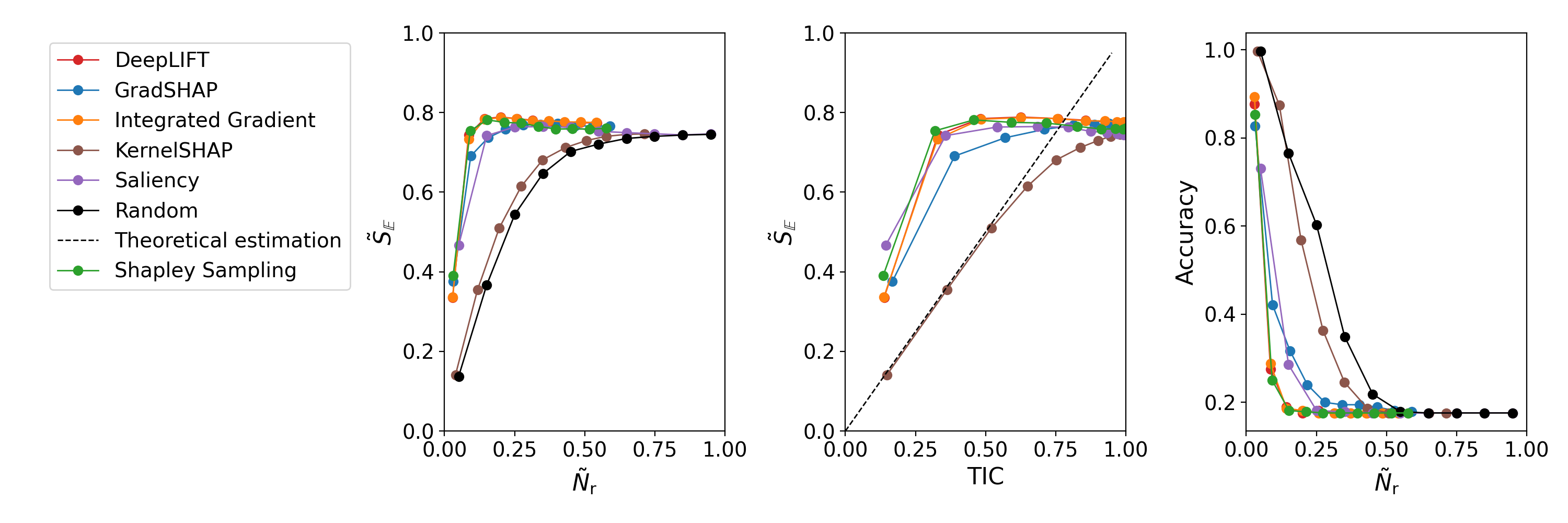
(a) CNN

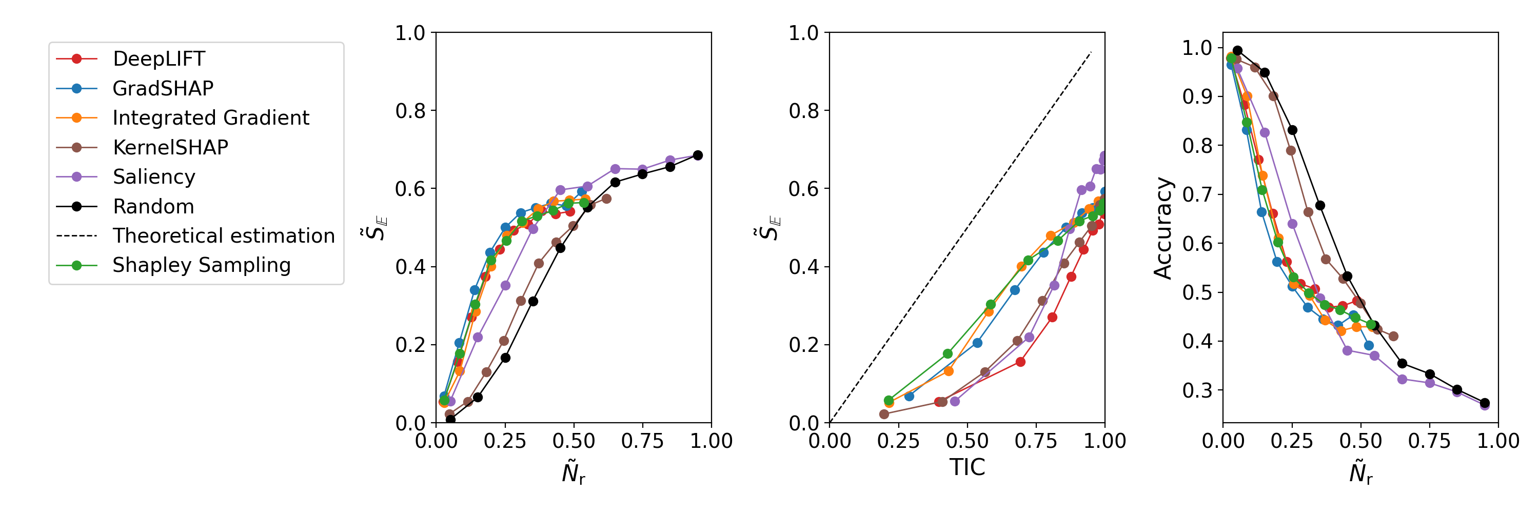
(b) Bi-LSTM

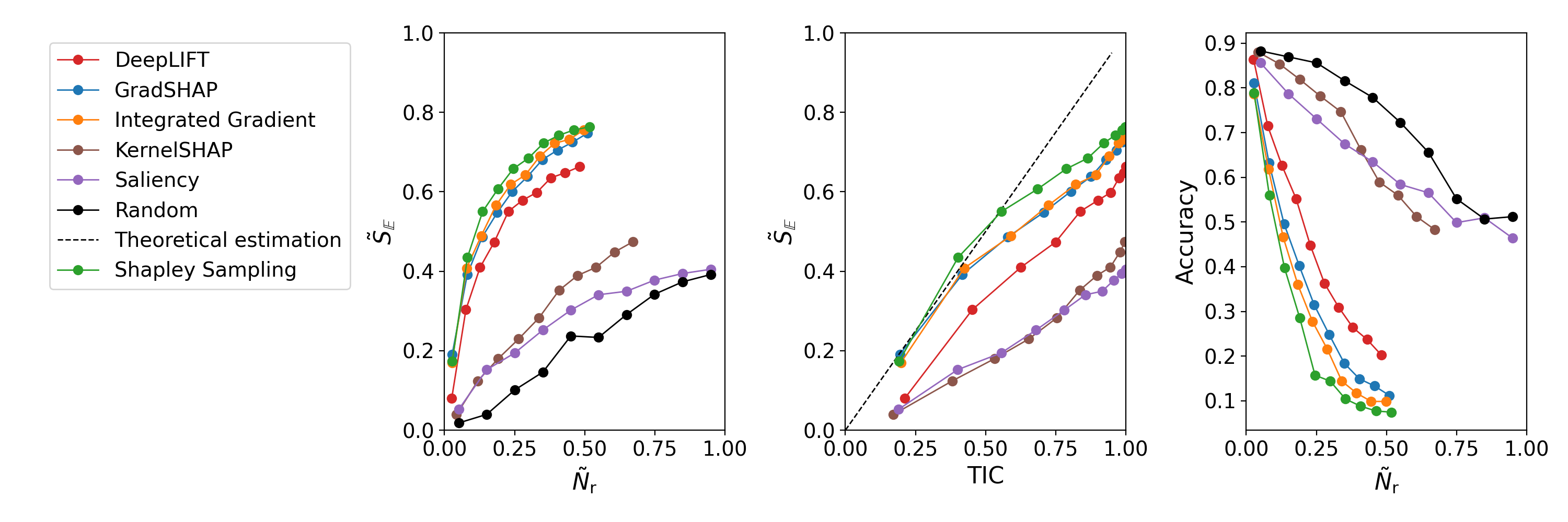
(c) Transformer

Extended data figure 5: Metrics $\tilde{S}_{\mathbb{E}}$ as a function of ratio of points removed (left column) and TIC (middle column), and accuracy as a function of ratio of points removed (right column), for (a) CNN, (b) bi-LSTM, and (c) transformer, using the synthetic dataset 3 (SD3) and permuting the time steps.

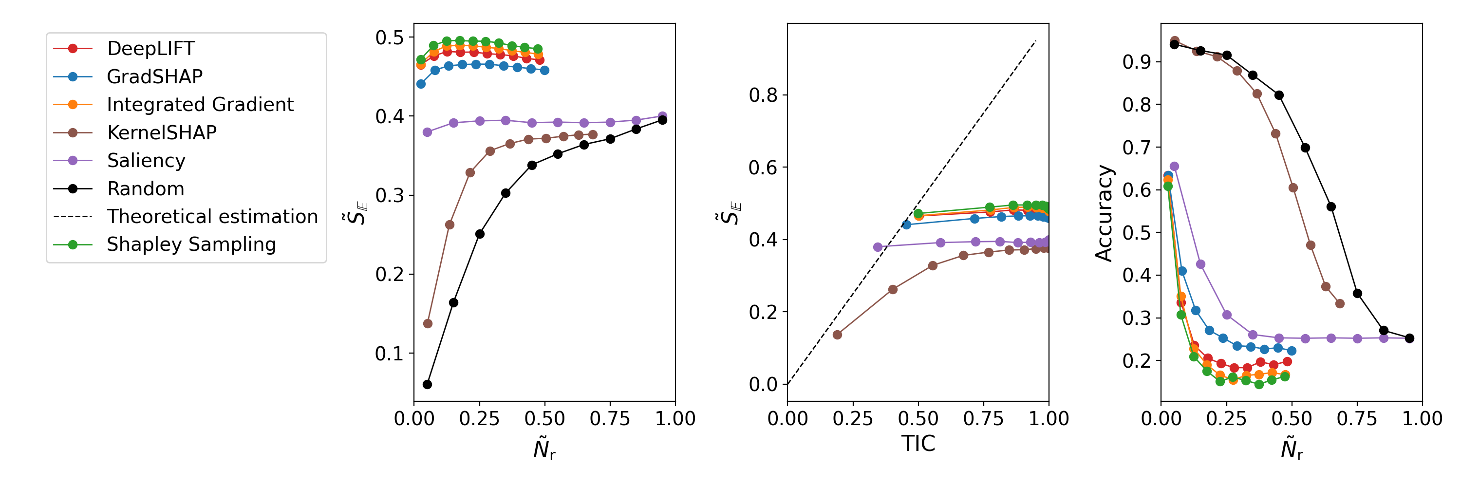
(a) CNN

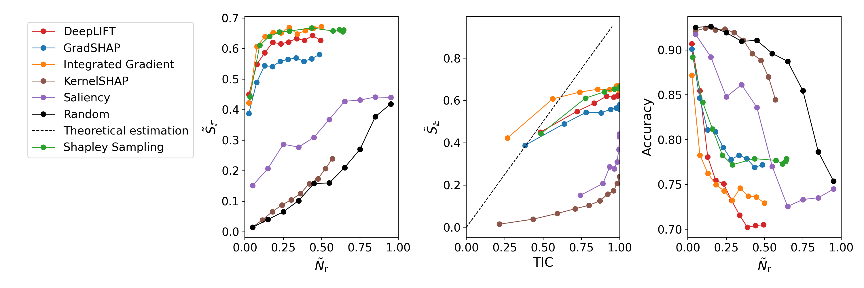
(b) Bi-LSTM

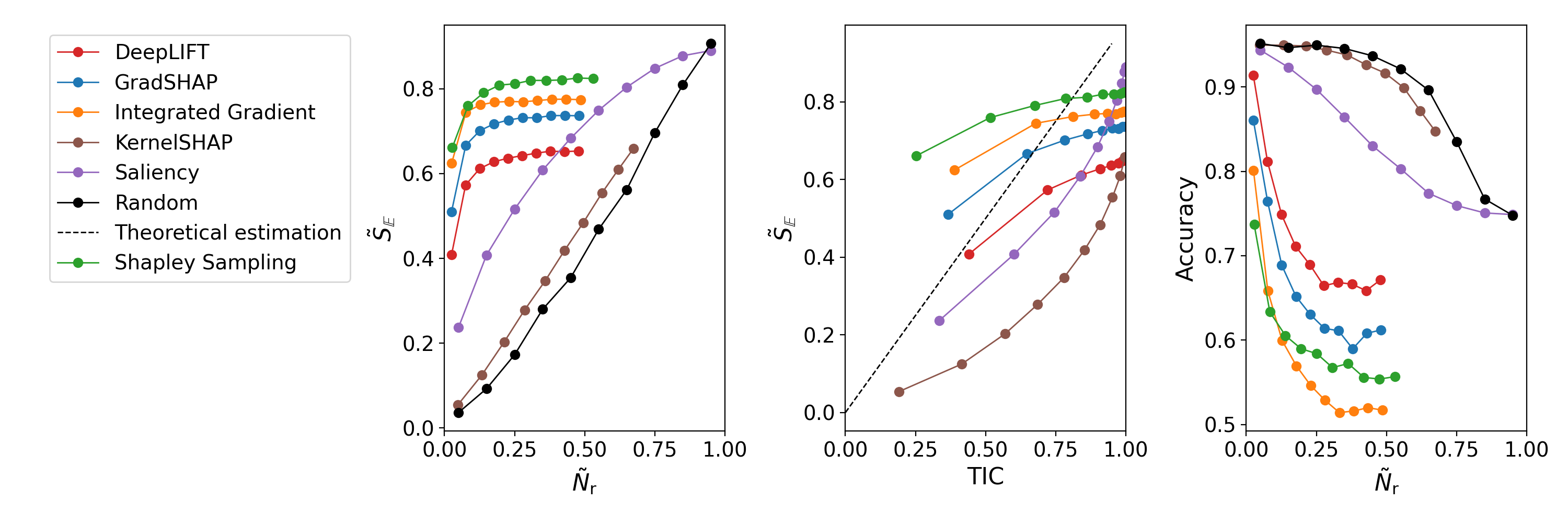
(c) Transformer

Extended data figure 6: Metrics $\tilde{S}_{\mathbb{E}}$ as a function of ratio of points removed $\tilde{N}_{\text{r}}$ (left column) and TIC (middle column), and accuracy as a function of ratio of points removed (right column), for (a) CNN, (b) bi-LSTM, and (c) transformer, using the ECG and normal sampling.

Extended data table 2: Evaluation of the interpretability metrics for the networks trained on the ECG datasets with signal being corrupted by permuting time steps (bold indicates the best performing interpretability method for each network).

	CNN	bi-LSTM	Transformer
DeepLift	0.361	0.307	0.597
GradShap	0.354	0.216	0.695
Integrated Gradients	0.366	0.283	0.746
KernelShap	0.300	0.139	0.401
Saliency	0.317	0.161	0.573
Shapley Sampling	0.367	0.270	0.776
Random	0.267	0.147	0.381

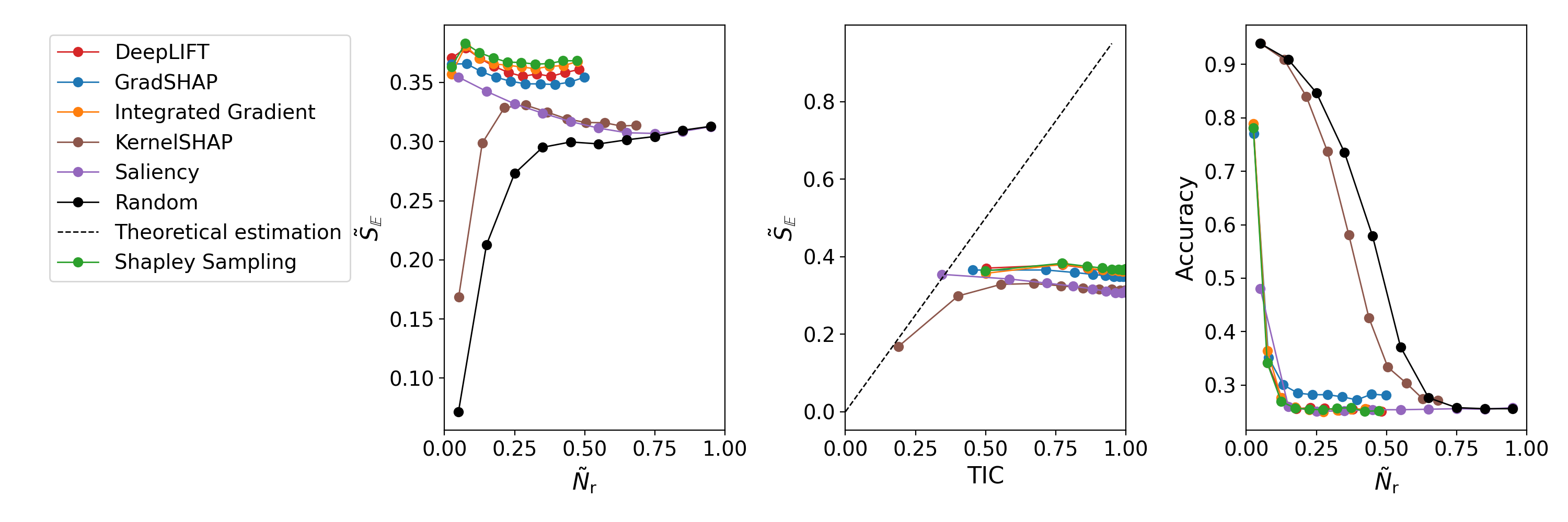
(a) CNN

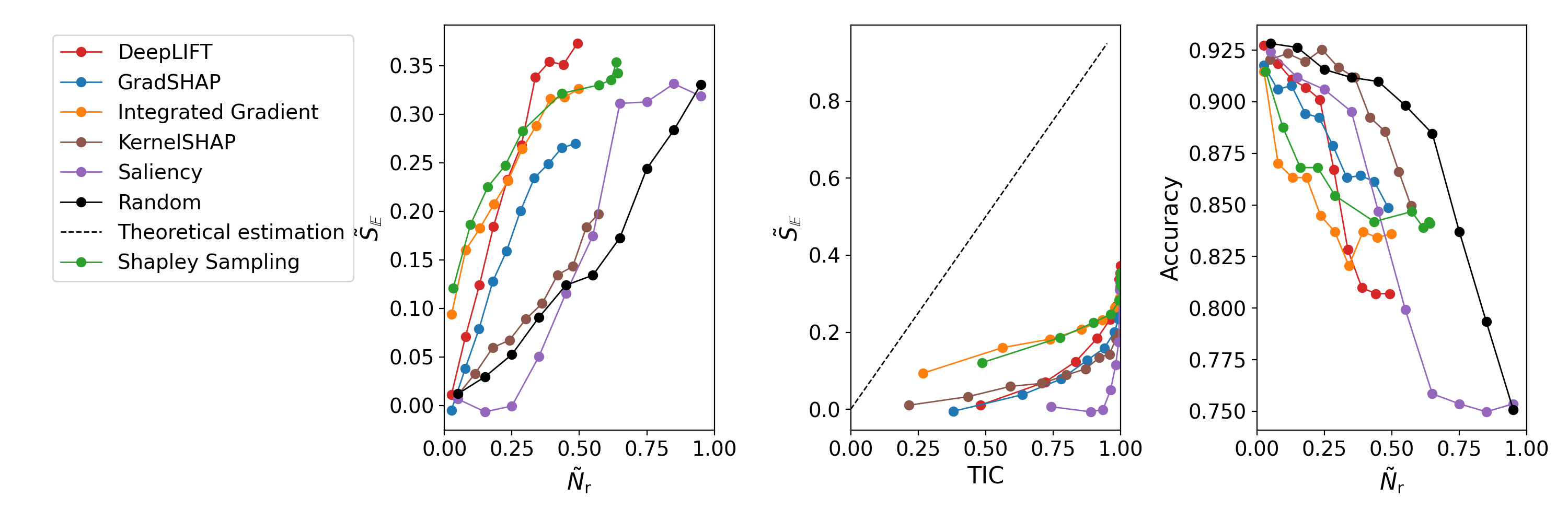
(b) Bi-LSTM

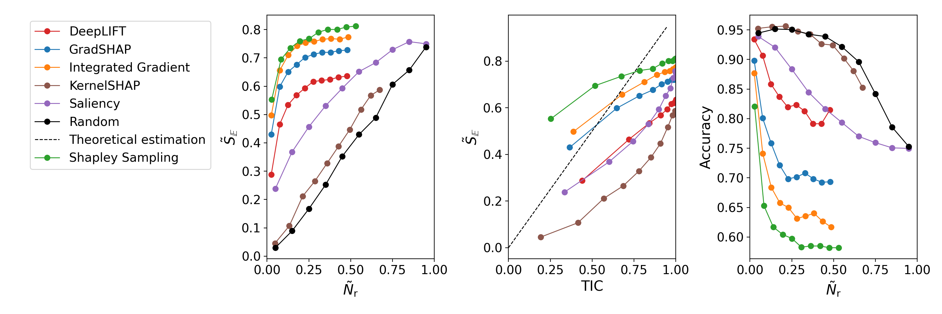
(c) Transformer

Extended data figure 7: Metrics $\tilde{S}_{\mathbb{E}}$ as a function of ratio of points removed (left column) and TIC (middle column), and accuracy as a function of ratio of points removed (right column), for (a) CNN, (b) bi-LSTM, and (c) transformer, using the ECG dataset and permuting the time steps.

Appendix

Appendix A Models’ configuration

A.1 Models trained on synthetic datasets

The configurations of the models trained on the synthetic datasets were chosen empirically to obtain near 100% accuracy. Three models per dataset were trained: CNN, bi-LSTM, and transformer. The same configuration for each type of network was retained across all synthetic datasets. All models were trained for a maximum of 200 epochs with an early stop criterion monitoring the loss on the validation set. In addition, all models were trained with the AdamW optimiser, an initial learning rate equal to $10^{-3}$ reducing by a factor of 10 when the validation loss plateaus. All networks were trained with a batch size equal to 128.

Table A1: CNN Models’ hyperparameters for the synthetic datasets

#	Layer	Parameters
1	Conv 1D	$64\times 7$, strides =1
2	Dropout	Rate =0.3
3	Conv 1D	$64\times 7$, strides =1
4	Dropout	Rate =0.3
5	Conv 1D	$64\times 7$, strides =1
6	Dropout	Rate =0.3
7	Average Pooling
8	Dense	units =5

Table A2: bi-LSTM Models’ hyperparameters for the synthetic datasets

#	Layer	Parameters
1	bi-LSTM	Units = 128
2	Dropout	Rate =0.2
3	bi-LSTM	Units = 128
4	Dropout	Rate =0.2
5	bi-LSTM	Units = 128
6	Dropout	Rate =0.2
7	Dense	Units =256, Activation = ReLU
8	Dense	Units =5

Table A3: Transformer Models’ hyperparameters for the synthetic datasets

#	Layer	Parameters
1	Dropout	Rate = 0.2
2	Dense	Units = 128
3	Positional encoding
4	Concatenate	Concatenate input and positional embedding
5	Transformer Encoder Layer	nb. of heads =8, dim. feedforward =256, dropout =0.3
6	Transformer Encoder Layer	nb. of heads =8, dim. feedforward =256, dropout =0.3
7	Transformer Encoder Layer	nb. of heads =8, dim. feedforward =256, dropout =0.3
8	Transformer Encoder Layer	nb. of heads =8, dim. feedforward =256, dropout =0.3
9	Average Pooling
10	Dense	Units =256, Activation = ReLU
11	Dense	Units =5

A.2 Models trained on the the ECG dataset

Hyper-parameter optimisations was performed in order to define the best parameters for each of the three model types across the search space described in table A4.

Table A4: Hyperparmeter search domain for the models trained on the ECG datasets

	Parameter	Search Space	Sampling
Common	learning rate	[1e-5,1e-2]	Loguniform
	batch size	[64, 128, 256]	Choice
	dropout	[0.1, 0.5]	Uniform
CNN	nb. Layers	[3,4]	Choice
	filters	[32, 64, 128, 256]	Choice
	kernel_size	[3,5,7,11,15]	Choice
bi-LSTM	nb. Layers	[3,4]	Choice
	filters	[32, 64, 128, 256]	Choice
Transformer	input dropout	[0,0.5]	Uniform
	nb encoder layer	[2,3,4,5]	Choice
	nb head	[2,4,8,16]	Choice
	Projection size	[64,128,256,512]	Choice
	MLP dim.	[64,128,256]	Choice

The hyperparameter search was performed using the Ray Tune library using Bayesian optimisation with 64 samples and HyperBand scheduler. Optimal training parameters for the three models are presented in table A5 while the optimal configuration for each model is presented in table A6, A7 and A8.

Table A5: Optimal parameters for models trained on the ECG dataset

	CNN	bi-LSTM	Transformer
Initial learning rate	5.85E-04	2.14E-04	1.82E-05
Batch size	256	256	256

Table A6: Optimal CNN configuration for the ECG dataset

#	Layer	Parameters
1	Conv 1D	$128\times 11$, strides =1
2	Dropout	Rate =0.307
3	Conv 1D	$256\times 11$, strides =1
4	Dropout	Rate =0.307
5	Conv 1D	$32\times 11$, strides =1
6	Dropout	Rate =0.307
7	Average Pooling
8	Dense	units =5

Table A7: Optimal bi-LSTM configuration for the ECG dataset

#	Layer	Parameters
1	bi-LSTM	Units = 64
2	Dropout	Rate =0.496
3	bi-LSTM	Units = 256
4	Dropout	Rate =0.496
5	bi-LSTM	Units = 32
6	Dropout	Rate =0.496
7	Dense	Units =256, Activation = ReLU
8	Dense	Units =5

Table A8: Transformer Model’s hyperparameters for the ECG dataset

#	Layer	Parameters
1	Dropout	Rate = 0.324
2	Dense	Units = 512
3	Positional encoding
4	Concatenate	Concatenate input and positional embedding
5	Transformer Encoder Layer	nb. of heads =8, dim. feedforward =256, dropout =0.265
6	Transformer Encoder Layer	nb. of heads =8, dim. feedforward =256, dropout =0.265
7	Transformer Encoder Layer	nb. of heads =8, dim. feedforward =256, dropout =0.265
9	Average Pooling
10	Dense	Units =128, Activation = ReLU
11	Dense	Units =5

Appendix B Classification Metrics

B.1 Syntetic datasets

Each synthetic dataset was split with a 0.7,0.15,0.15 split between the train, validation and test set. Accuracy for the three model types and across the three synthetic datasets are presented in table B1.

Table B1: Classification accuracy across the 3 synthetic datasets for the train, validation (valid.) and test set

	CNN			Bi-LSTM			Transformer
	Train	Valid.	Test	Train	Valid.	Test	Train	Valid.	Test
Dataset 1	1.00	1.00	1.00	0.99	1.00	0.98	1.00	0.94	0.93
Dataset 2	1.00	1.00	1.00	1.00	1.00	1.00	1.00	0.95	0.94
Dataset 3	1.00	1.00	1.00	1.00	0.99	0.99	1.00	0.87	0.89

B.2 ECG

Accuracy along the precision and recall are presented for the classification task on the ECG dataset in table B2. In addition confusion matrices for the three models are presented in figure B1, B2 and B3.

Table B2: Classification metrics for the 3 models trained on the ECG test reported for the train, validation (valid.) and test set

	CNN			Bi-LSTM			Transformer
	Train	Valid.	Test	Train	Valid.	Test	Train	Valid.	Test
Accuracy	0.971	0.938	0.955	0.904	0.903	0.919	0.947	0.951	0.953
Precision	0.926	0.860	0.879	0.849	0.838	0.847	0.880	0.876	0.876
Recall	0.973	0.916	0.954	0.790	0.789	0.831	0.933	0.949	0.950
F1	0.949	0.887	0.915	0.819	0.813	0.839	0.906	0.911	0.911

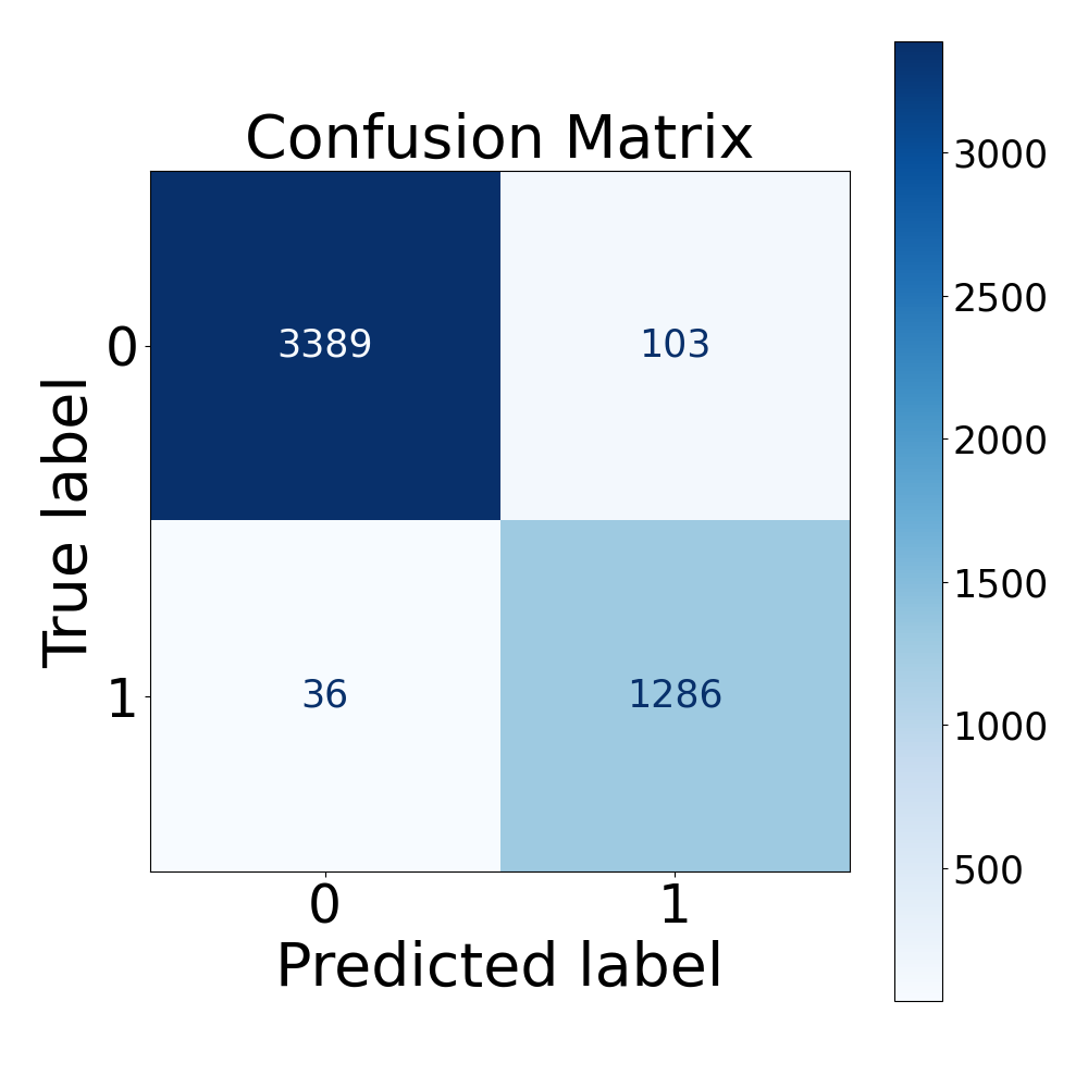
(a) Train

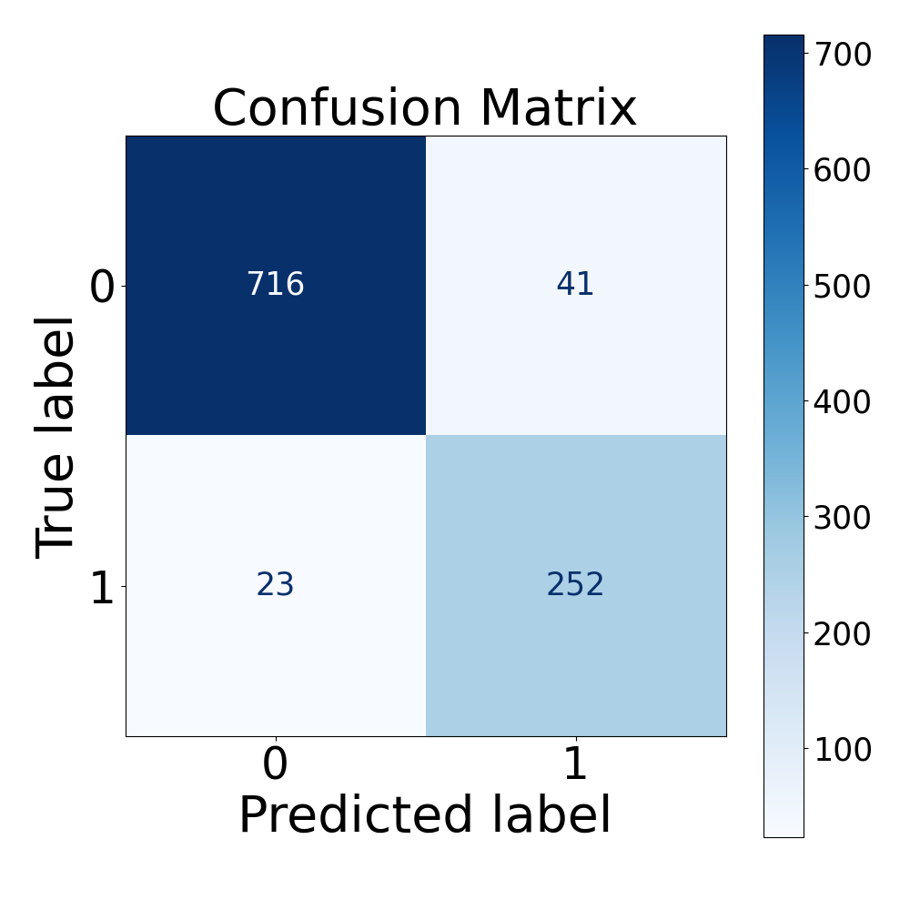
(b) Validation

(c) Test

Figure B1: Confusion matrix for the CNN model trained on the ECG task for the train, validation and test set

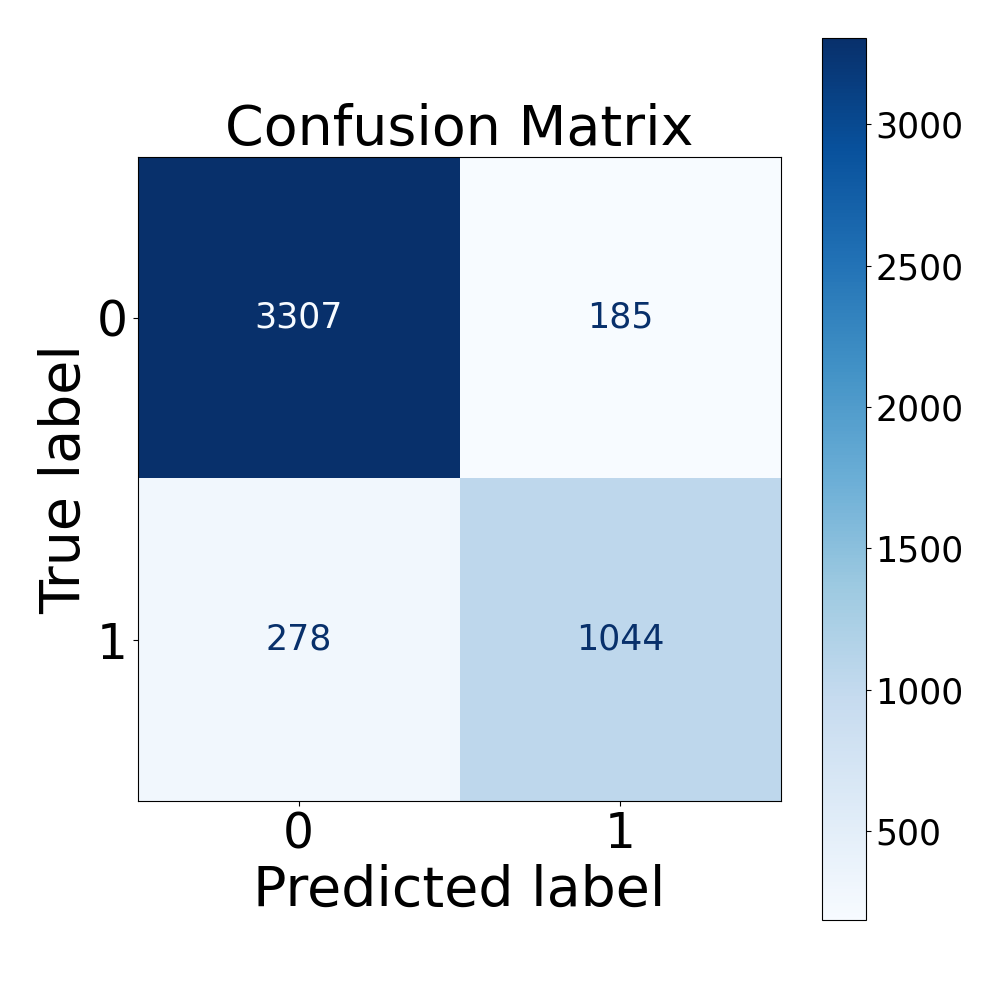
(a) Train

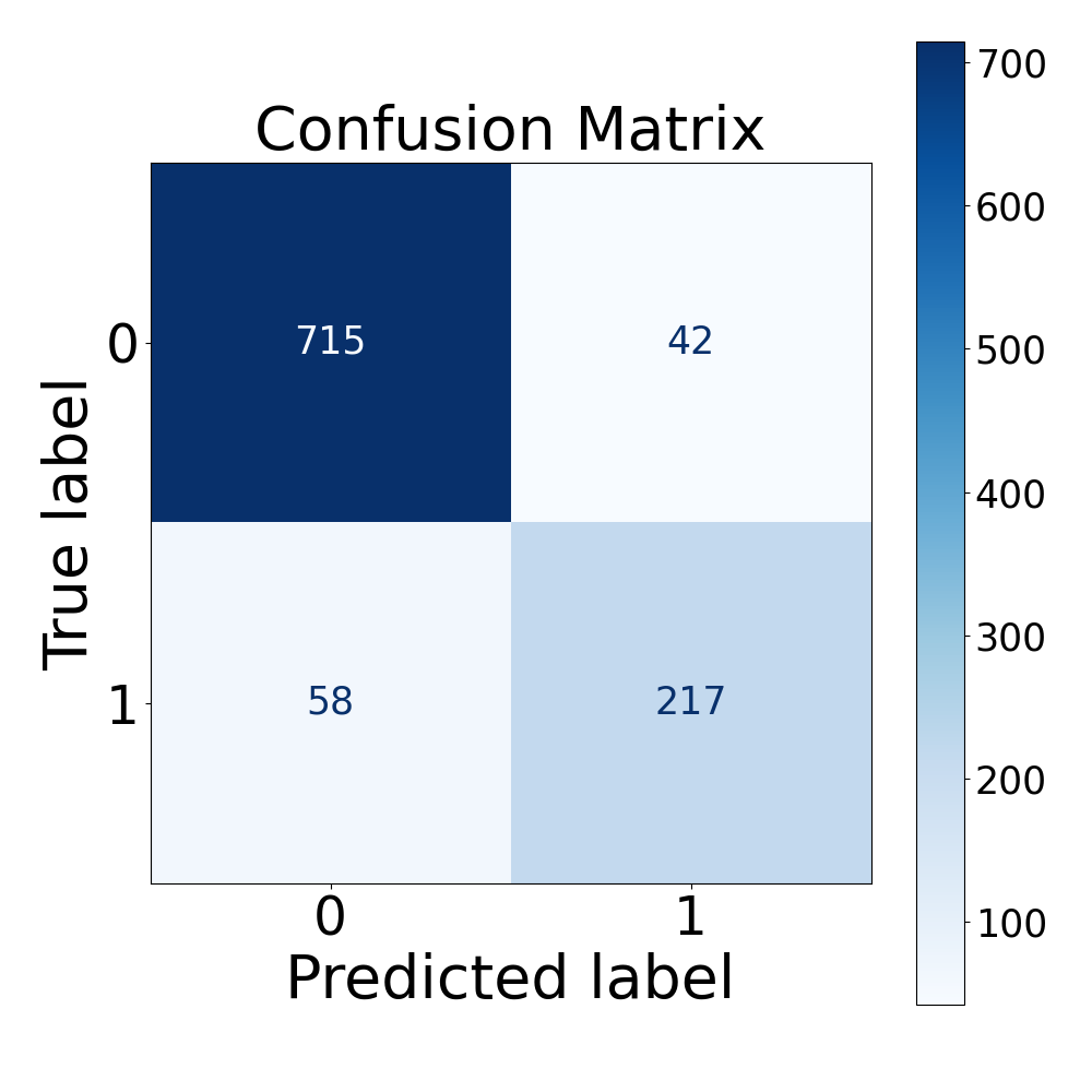
(b) Validation

(c) Test

Figure B2: Confusion matrix for the bi-LSTM model trained on the ECG task for the train, validation and test set

(a) Train

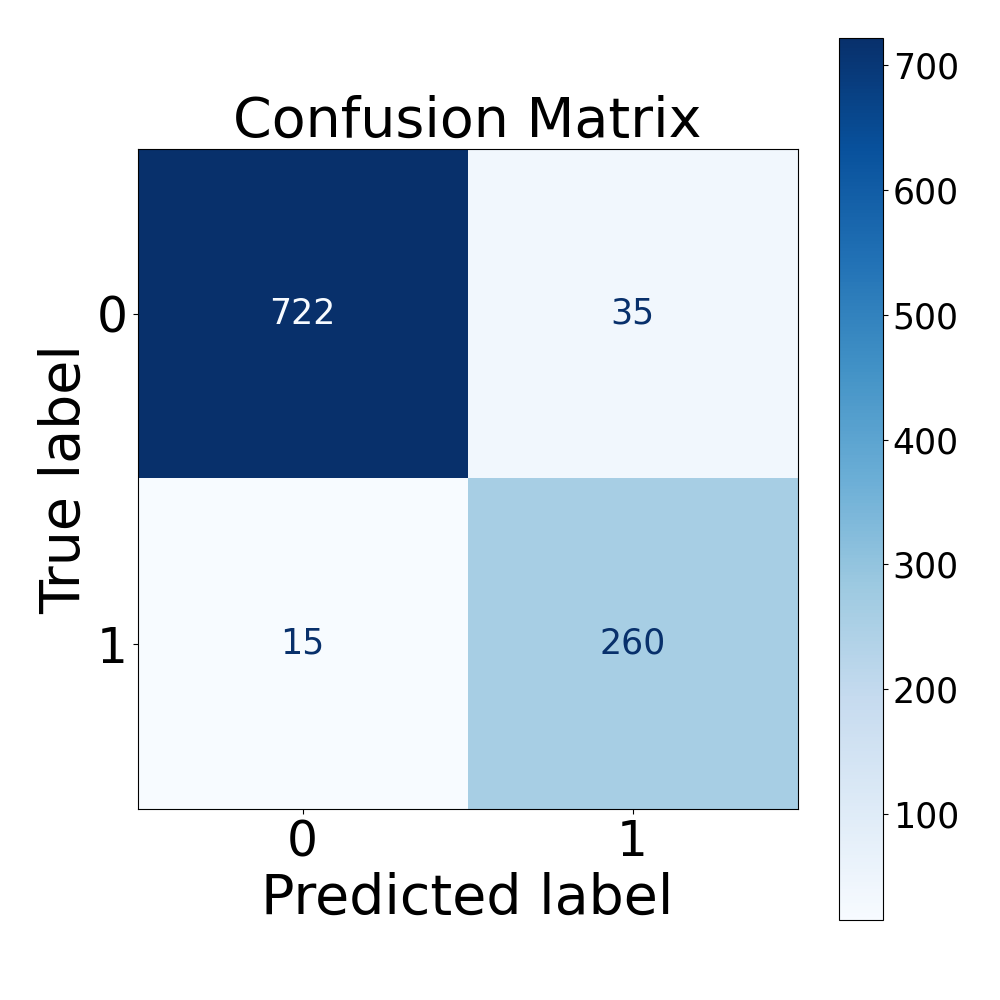
(b) Validation

(c) Test

Figure B3: Confusion matrix for the Transformer model trained on the ECG task for the train, validation and test set

References

- [1] Weyn JA, Durran DR, Caruana R. Improving Data-Driven Global Weather Prediction Using Deep Convolutional Neural Networks on a Cubed Sphere. Journal of Advances in Modeling Earth Systems. 2020 Sep;12(9). Available from: https://onlinelibrary.wiley.com/doi/10.1029/2020MS002109.
- [2] Yang R, Yu L, Zhao Y, Yu H, Xu G, Wu Y, et al. Big data analytics for financial Market volatility forecast based on support vector machine. International Journal of Information Management. 2020 Feb;50:452-62. Available from: https://linkinghub.elsevier.com/retrieve/pii/S0268401218313604.
- [3] Rajkomar A, Oren E, Chen K, Dai AM, Hajaj N, Hardt M, et al. Scalable and accurate deep learning with electronic health records. NPJ Digital Medicine. 2018;1(1):1-10.
- [4] Hewamalage H, Bergmeir C, Bandara K. Recurrent neural networks for time series forecasting: Current status and future directions. International Journal of Forecasting. 2021;37(1):388-427.
- [5] Fawaz HI, Forestier G, Weber J, Idoumghar L, Muller PA. Deep learning for time series classification: a review. Data Mining and Knowledge Discovery. 2019;33(4):917-63.
- [6] Lipton ZC. The Mythos of Model Interpretability. arXiv:160603490 [cs, stat]. 2017 Mar. ArXiv: 1606.03490. Available from: http://arxiv.org/abs/1606.03490.
-
[7]
European Commission C Directorate-General for Communications Networks,
Technology. Proposal for a regulation of the European parliament and of the
council laying down harmonised rules on artificial intelligence (artificial
intelligence act) and amending certain union legislative acts COM/2021/206
final; 2021.
http://https://eur-lex.europa.eu/legal-content/EN/ALL/?uri=CELEX:52021PC0206. - [8] Shad R, Cunningham JP, Ashley EA, Langlotz CP, Hiesinger W. Designing clinically translatable artificial intelligence systems for high-dimensional medical imaging. Nature Machine Intelligence. 2021 Nov;3(11). Available from: https://www.nature.com/articles/s42256-021-00399-8.
- [9] Kokhlikyan N, Miglani V, Martin M, Wang E, Alsallakh B, Reynolds J, et al.. Captum: A unified and generic model interpretability library for PyTorch; 2020.
- [10] Montavon G, Bach S, Binder A, Samek W, Müller KR. Explaining NonLinear Classification Decisions with Deep Taylor Decomposition. Pattern Recognition. 2017 May;65:211-22. ArXiv: 1512.02479. Available from: http://arxiv.org/abs/1512.02479.
- [11] Lundberg SM, Lee SI. A Unified Approach to Interpreting Model Predictions. In: Guyon I, Luxburg UV, Bengio S, Wallach H, Fergus R, Vishwanathan S, et al., editors. Advances in Neural Information Processing Systems 30. Curran Associates, Inc.; 2017. p. 4765-74. Available from: http://papers.nips.cc/paper/7062-a-unified-approach-to-interpreting-model-predictions.pdf.
- [12] Neves I, Folgado D, Santos S, Barandas M, Campagner A, Ronzio L, et al. Interpretable heartbeat classification using local model-agnostic explanations on ECGs. Computers in Biology and Medicine. 2021;133:104393.
- [13] Jacovi A, Goldberg Y. Towards faithfully interpretable NLP systems: How should we define and evaluate faithfulness? arXiv preprint arXiv:200403685. 2020.
- [14] Adebayo J, Gilmer J, Muelly M, Goodfellow I, Hardt M, Kim B. Sanity checks for saliency maps. arXiv preprint arXiv:181003292. 2018.
- [15] Samek W, Binder A, Montavon G, Lapuschkin S, Müller KR. Evaluating the visualization of what a deep neural network has learned. IEEE transactions on neural networks and learning systems. 2016;28(11):2660-73.
- [16] Hooker S, Erhan D, Kindermans PJ, Kim B. A Benchmark for Interpretability Methods in Deep Neural Networks. arXiv:180610758 [cs, stat]. 2019 Nov. ArXiv: 1806.10758. Available from: http://arxiv.org/abs/1806.10758.
- [17] Schlegel U, Arnout H, El-Assady M, Oelke D, Keim DA. Towards a rigorous evaluation of xai methods on time series. In: 2019 IEEE/CVF International Conference on Computer Vision Workshop (ICCVW). IEEE; 2019. p. 4197-201.
- [18] Ismail AA, Gunady M, Bravo HC, Feizi S. Benchmarking Deep Learning Interpretability in Time Series Predictions. arXiv:201013924 [cs, stat]. 2020 Oct. ArXiv: 2010.13924. Available from: http://arxiv.org/abs/2010.13924.
- [19] Shrikumar A, Greenside P, Kundaje A. Learning Important Features Through Propagating Activation Differences. arXiv:170402685. 2017.
- [20] Sundararajan M, Taly A, Yan Q. Axiomatic Attribution for Deep Networks. arXiv:13126034[cs]. 2017.
- [21] Simonyan K, Vedaldi A, Zisserman A. Deep inside convolutional networks: Visualising image classification models and saliency maps. arXiv preprint arXiv:13126034. 2013.
- [22] Castro J, Gómez D, Tejada J. Polynomial calculation of the Shapley value based on sampling. Computers & Operations Research. 2009;36(5):1726-30. Selected papers presented at the Tenth International Symposium on Locational Decisions (ISOLDE X). Available from: https://www.sciencedirect.com/science/article/pii/S0305054808000804.
- [23] Hughes JW, Olgin JE, Avram R, Abreau SA, Sittler T, Radia K, et al. Performance of a convolutional neural network and explainability technique for 12-lead electrocardiogram interpretation. JAMA cardiology. 2021;6(11):1285-95.
- [24] Bodini M, Rivolta MW, Sassi R. Opening the black box: interpretability of machine learning algorithms in electrocardiography. Philosophical Transactions of the Royal Society A. 2021;379(2212):20200253.
- [25] Surawicz B, Childers R, Deal BJ, Gettes LS. AHA/ACCF/HRS Recommendations for the Standardization and Interpretation of the Electrocardiogram: Part III: Intraventricular Conduction Disturbances A Scientific Statement From the American Heart Association Electrocardiography and Arrhythmias Committee, Council on Clinical Cardiology; the American College of Cardiology Foundation; and the Heart Rhythm Society Endorsed by the International Society for Computerized Electrocardiology. Journal of the American College of Cardiology. 2009;53(11):976-81. Available from: https://www.sciencedirect.com/science/article/pii/S0735109708041351.
- [26] Chua LO. The Genesis of Chua’s Circuit. EECS Department, University of California, Berkeley; 1992. UCB/ERL M92/1. Available from: http://www2.eecs.berkeley.edu/Pubs/TechRpts/1992/1924.html.
- [27] Abell ML, Braselton JP. Introductory Differential Equations. Academic Press; 2018.
- [28] Lorenz EN. Deterministic nonperiodic flow. Journal of atmospheric sciences. 1963;20(2):130-41.
- [29] Rikitake T. Oscillations of a system of disk dynamos. In: Mathematical Proceedings of the Cambridge Philosophical Society. vol. 54. Cambridge University Press; 1958. p. 89-105.
- [30] Rössler OE. An equation for continuous chaos. Physics Letters A. 1976;57(5):397-8. Available from: https://www.sciencedirect.com/science/article/pii/0375960176901018.
- [31] Matsumoto T. A chaotic attractor from Chua’s circuit. IEEE Transactions on Circuits and Systems. 1984;31(12):1055-8.
- [32] Liu F, Liu C, Zhao L, Zhang X, Wu X, Xu X, et al. An Open Access Database for Evaluating the Algorithms of Electrocardiogram Rhythm and Morphology Abnormality Detection. Journal of Medical Imaging and Health Informatics. 2018 Sep;8(7):1368-73. Available from: https://doi.org/10.1166/jmihi.2018.2442.
- [33] Bussink BE, Holst AG, Jespersen L, Deckers JW, Jensen GB, Prescott E. Right bundle branch block: prevalence, risk factors, and outcome in the general population: results from the Copenhagen City Heart Study. European Heart Journal. 2012 09;34(2):138-46. Available from: https://doi.org/10.1093/eurheartj/ehs291.
- [34] Carreiras C, Alves AP, Lourenço A, Canento F, Silva H, Fred A, et al.. BioSPPy: Biosignal Processing in Python; 2015–. [Online; accessed 2021 May]. Available from: https://github.com/PIA-Group/BioSPPy/.