Bernstein Flows for Flexible Posteriors in Variational Bayes

Bernstein Flows for Flexible Posteriors in Variational Bayes

Abstract

Variational inference (VI) is a technique to approximate difficult to compute posteriors by optimization. In contrast to MCMC, VI scales to many observations. In the case of complex posteriors, however, state-of-the-art VI approaches often yield unsatisfactory posterior approximations. This paper presents Bernstein flow variational inference (BF-VI), a robust and easy-to-use method, flexible enough to approximate complex multivariate posteriors. BF-VI combines ideas from normalizing flows and Bernstein polynomial-based transformation models. In benchmark experiments, we compare BF-VI solutions with exact posteriors, MCMC solutions, and state-of-the-art VI methods including normalizing flow based VI. We show for low-dimensional models that BF-VI accurately approximates the true posterior; in higher-dimensional models, BF-VI outperforms other VI methods. Further, we develop with BF-VI a Bayesian model for the semi-structured Melanoma challenge data, combining a CNN model part for image data with an interpretable model part for tabular data, and demonstrate for the first time how the use of VI in semi-structured models.

I Introduction

Uncertainty quantification is essential, especially if model predictions are used to support high stake decision-making. Quantifying uncertainty in statistical or machine learning models is often achieved by Bayesian approaches, where posterior distributions represent the uncertainty of the estimated model parameters. Determining these posterior distributions exactly is usually impossible if the posterior takes a complex shape and if the model has many parameters, such as a Bayesian neural network (NN), or semi-structured models combining an interpretable model part with deep NNs. Variational inference (VI) is a commonly used approach to approximate complex distributions through optimization [1, 2, 3]. In VI, the posterior is approximated by minimizing a divergence between the variational distribution and the posterior.

VI is currently a very active research field tackling different challenges, which can be categorized into the following groups: (1) constructing variational distributions that are flexible enough to match the true posterior distribution, (2) defining suited variational objective for tuning the variational distribution, which boils down to finding the most suited divergence measure quantifying the difference between a variational distribution and posterior, and (3) developing robust and accurate stochastic optimization frameworks for the variational objective [4, 5]. Here, we focus on challenge (1) and propose a method to construct a variational distribution that is flexible enough to accurately approximate complex posteriors while being robust and easy to use, since it can be used in a black-box VI fashion and so requires no problem-specific calculations [6].

Usually, the variational distribution is constructed by first choosing a family of parametric distributions, often Gaussians, and then tuning the parameters to minimize the divergence to the posterior. Obviously, the quality of the VI approximation depends on the similarity of the true posterior with the optimized member of the chosen distribution family. In cases where the posterior takes a complex shape, a simple variational distribution, such as a Gaussian, can never yield a good approximation. Mixtures of simple distributions are often used to construct complex distributions but they require choosing an appropriate number of components and have problems fitting skewed distributions. More recently, transformation models (TMs) and normalizing flows (NF) were developed to construct complex distributions. Both, TMs and NFs, rely on the same principle idea, i.e., fitting a strictly monotone function that transforms between a pre-defined simple distribution and a potentially complex target distribution. TMs and NFs were developed independently from each other in the statistics and machine learning community and differ mainly in the construction of the transformation function. NFs were inspired by neural networks and the transformation function usually is constructed by chaining many simple functions. On the other hand, TMs were inspired by flexible statistical models and often use Bernstein polynomials to construct a flexible transformation function.

We propose Bernstein flow variational inference (BF-VI) using ideas from Bernstein polynomial based TMs for constructing a variational distribution that closely approximates a potentially complex posterior in Bayesian models. We demonstrate how this can be achieved via a computationally efficient, batch-capable optimization process applicable to typical statistical and neural network based models on arbitrary large datasets. Since deep Bayesian NNs do not require flexible VI distribution [7], we here focus on the benefit of BF-VI for models with a moderate number of interpretable parameters. We further demonstrate for the first time how VI can be used to fit Bayesian semi-structured models where interpretable statistical model parts, based on tabular data, and deep NN model parts, based on images, are jointly fitted. We benchmark our BF-VI approach against exact Bayesian models, MCMC-Simulations, Gaussian-VI , and NF-VI, showing accurate posterior approximations in low dimensions and superior or equal approximations in higher dimensions when compared to Gaussian-VI or NF-VI.

II Related Work

Normalizing flows (NF) were developed in the deep learning community and, interestingly, originally proposed for variational inference [8]. However, since then, NF have been mainly used for other applications (see [9] for a recent review). NF became prominent for their ability to fit complex and high dimensional distributions from which new samples can be generated, which was e.g. used for creating impressive realistic samples of pictures of human faces [10], or human voices [11]. In deep learning models, NF were used to approximate the posterior of the latent variables [8] and, indirectly, by constructing a flexible mixing density, to build the variational distribution of the weights from multivariate Gaussians [12]. In a recent study [13] NF has been used for the first time for VI, but with inferior performance compared to other state-of-the art VI methods.

The main idea of NFs is to fit a potentially complex and high-dimensional target distribution by learning a flexible but strictly monotone transformation function that transforms a simple base distribution, such as the Standard Gaussian $N(0,1)$, to the target distribution. In NF, the transformation function is usually constructed by chaining many simple strictly monotone transformations, like shift and scale transformations. The needed flexibility is obtained by stacking many of such operations. However, there were also approaches proposed which use a single flexible transformation, such as sum-of-squares polynomials [14], or splines [15].

Independently to NFs and at the same time, transformation models were developed in statistics [16] focusing on modeling a potentially complex conditional outcome distribution in regression models. Also in TMs a flexible and strictly monotone transformation function is learned that transforms between a simple base distribution and a potentially complex conditional outcome distribution. While the choice of the simple base distribution is unimportant for modeling unconditional distributions or for pure prediction purposes, it gets crucial for inference in regression models where e.g., a standard-logistic base distribution allows to interpret the regression coefficients as log-odds-ratios [17, 18].

In TMs, the potentially complex and strictly monotone transformation function is parameterized as an expansion of basis functions. In the case of continuous target distributions, most often, Bernstein polynomials [19] are used because they can easily be constrained to be strictly monotone and their flexibility can be tuned via their order. A large order $M$ ensures an accurate approximation of the distribution, which is robust against a further increase of $M$ [17], demonstrated also in our experiments.

TMs were also used for discrete outcome distribution, but here Bernstein polynomials are not suitable because the transformation function needs to be discrete [18, 20, 21]. While TMs have the focus on regression models [16] they were also successfully used for modeling unconditional and high dimensional distributions [22]. Also in NN models, TMs based on Bernstein polynomials have been used to model complex one-dimensional conditional distributions [21, 23, 24] or unconditional multidimensional distributions [25].

While it is obvious that TMs or NFs have the potential to construct flexible variational distributions to accurately approximate potentially complex posterior distributions, TMs have not been used for VI yet and first attempts of NF-based VI [13] compares unfavorable against other VI methods. To the best of our knowledge we are the first to use Bernstein polynomials based TMs for VI which we call BF-VI. We show the applicability of BF-VI for single- and multi-parameter models, e.g., in a regression model with 26 parameters (see diamond example in IV-B). However, in models with a huge amount of parameters, such as deep BNNs, it is extremely hard to optimize a joint variational distribution over all parameters. Therefore, BNNs are often fitted with mean-field (MF) VI ignoring dependencies between the model parameters. Fortunately, this seems not to be a problem since it was demonstrated for VI with Gaussian variational distributions that MF-Gaussian-VI and full Gaussian-VI, incorporating dependencies, achieved in deeper NNs the same quality in terms of the modeled outcome distribution [7]. Hence, the authors form [7] concluded that deep BNNs do not need complex weight posterior approximations, which they summarize as ”liberty or depth”. This leaves the focus on models with a moderate number ($<100$) of interpretable parameters, on which we focus in our study. This includes pure statistical models and semi-structured models combining deep NNs and interpretable model components.

III Methods

In the following, we describe the Bernstein-Flow-VI approach, which we propose for accurate and robust approximating potentially complex posteriors in Bayesian models. The code is publicly available on github. The main idea is to enable the VI procedure to approximate the posterior of the model parameters by a flexible variational distribution. We first explain the one-dimensional version of the Bernstein-flow and then generalize to multivariate distribution.

III-A One Dimensional Berstein-Flows

The heart of our method is the Bernstein-Flow, a bijective (w.l.o.g. strictly monotone increasing), function $f_{\text{BP}}:Z\rightarrow\theta$ that approximates the bijective transformation function $g:Z\rightarrow\theta$ between a random variable $Z$ with a simple cumulative distribution function (CDF) $F_{Z}$ and $\theta$ with a potentially complex CDF $F_{\theta}$ so that $F_{Z}(z)=F_{\theta}(g(z))$. In our application the corresponding density of $F_{\theta}$ is the posterior $p(\theta|D)$ and its approximation corresponds to the variational distribution $q_{\text{\boldmath$\lambda$}}(\theta)$, where the parameters of the $f_{\text{BP}}$ are the variational parameters $\lambda$. Hothorn et al. [17] give theoretical guarantees for the existence and uniqueness of $g=F_{\theta}^{-1}\circ F_{Z}$. We approximate $g$ with a flow function $f_{\text{BP}}$ that we construct via polynomials in Bernstein form (BP) as

$$\small g(z)\approx f_{\text{BP}}(z)=\sum_{i=0}^{M}{\operatorname{Be}_{i}(z)\frac{\vartheta_{i}}{M+1}}$$ (1)

with $\operatorname{Be}_{i}(z^{\prime})=\operatorname{Be}_{(i+1,M-i+1)}(z^{\prime})$ being the density of the Beta distribution. The input $z$ needs to be within $[0,1]$, which can be guarantied by using e.g. a truncated Gaussian for $F_{Z}$. Using a BP for approximating $g$ gives the following theoretical guarantees [26] (1) With increasing order $M$ of the BP, the approximation $f_{\text{BP}}$ to $g$ gets arbitrarily close (the BP have been introduced for this very purpose in the constructive proof of the Weierstrass theorem by [19]); (2) the required strict monotonicity of the approximation $f_{\text{BP}}$ can be easily achieved by constraining the coefficients $\vartheta_{i}$ of the BP to be increasing; 3) BPs are robust versus perturbations of the coefficients $\vartheta_{i}$; 4) the approximation error decreases with $1/M$ (Voronovskaya Theorem). See [19, 26] for more detailed discussions of the beneficial properties of BPs in general and [17, 25] for transformation models.

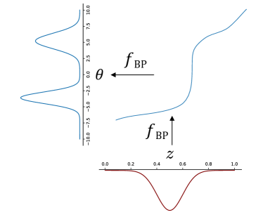
Figure 1: Overview of the bijective transformation $f_{\text{BP}}$ mapping between a simple distribution (lower right) and a potentially complex variational distribution $q_{\lambda}(\theta)$ (upper left). The transformation $f_{\text{BP}}$ is given by (1).

While a BP is in principle sufficient to approximate $g$ accurately, we have observed in low dimensional examples a more efficient training when sandwiching the $f_{\text{BP}}$ with two monotone increasing linear functions $l_{1}$ and $l_{2}$. In this case, the support $[0,1]$ for the BP is guaranteed by a sigmoid transformation $\sigma$ directly before the BP transformation resulting in a flow $f=l_{2}\circ f_{\text{BP}}\circ\sigma\circ l_{1}$. The flow $f:Z\rightarrow\theta$ starts with $l_{1}(z)=\alpha\cdot z+b$, followed by $\text{BP}\circ\sigma:l_{1}(z)\rightarrow\theta^{\prime}$ and ending with $\theta=l_{2}(\theta^{\prime})=\alpha\cdot\theta^{\prime}+\beta$. This sandwich construction allows to choose a simple distributions $F_{z}$ which does not need to have the support $[0,1]$ such as the Standard-Normal.

To allow the application of unconstrained SGD-optimization, we enforce the strict monotonicity of the flow $f$ as follows: We optimze unrestricted parameters $\vartheta_{0}^{\prime},\ldots\vartheta_{M}^{\prime}$ and, in case of sandwiching linear transformations, additional parameters $a^{\prime},b,\alpha^{\prime},\beta$ and apply the following transformations to determine the parameters of the bijective flow: $\vartheta_{0}=\vartheta_{0}^{\prime}$, and $\vartheta_{i}=\vartheta_{i-1}+\operatorname{softplus}(\vartheta_{i}^{\prime})$ for $i=1,\dots,M$ for getting an strictly increasing BP and $a=\operatorname{softplus}(a^{\prime})$ and $\alpha=\operatorname{softplus}(\alpha^{\prime})$, for getting increasing linear transformations.

In the appendix we show that the resulting variational distribution is a tight approximation to the posterior in the sense that the KL divergence between $q_{\lambda}(\theta)$ and $p(\theta|D)$ decreases with the order of the BP via $1/M$.

III-B Multivariate Generalization

In the case of a Bayesian model with $p$ parameters, $\theta_{1},\theta_{2},\ldots,\theta_{p}$, the Bernstein-Flow bijectively maps a $p$-dimensional $\mathbf{Z}$ to a $p$-dimensional $\theta$. To model the multivariate flow $\text{\boldmath$f$}_{\text{BP}}:\text{$\mathbf{Z}$}\rightarrow\text{\boldmath$\theta$}$, we construct a triangular map using a masked autoregressive flow (MAF) [27]. The MAF gets as input $z$ and outputs the coefficients of $p$ BPs that are used to determine the $p$ components of $\theta$. The MAF architecture ensures that the coefficients ${\vartheta_{i}^{j}}$ $j=2,\ldots p\;,i=0,\cdots,M$ of the $j$-th BP determining $\theta_{j}$ only depends on the first $j$-1 components of $z$.

$$\theta_{j}=f_{\text{BP}_{j}}(z_{1:k\leq j})=\frac{1}{M+1}\sum_{i=0}^{M}\vartheta_{i}^{j}(z_{1},\ldots,z_{j-1})\operatorname{Be}_{i}(z_{j})$$

Since the Jacobian $\nabla{\text{\boldmath$f$}_{\text{BP}}}$ is a triangular matrix, $\det\nabla{\text{\boldmath$f$}_{\text{BP}}}$ is given by the product of the diagonal elements of the Jacobian. The resulting $p$-dimensional variational distribution $q_{\text{\boldmath$\lambda$}}(\text{\boldmath$\theta$})$ can be determined via the change of variable formula (see (5)). The flexibility of such a $p$-dimensional bijective Bernstein-flow is only limited by the order $M$ of the Bernstein polynomial and the complexity of the MAF. It is known that bijective triangular maps with sufficient flexibility can map a simple $p$-dimensional distribution into arbitrary complex $p$-dimensional target distributions [28]. In our experiments, we use a MAF with two hidden layers, each with 10 neurons. The weights $w$ of the MAF are the variational parameters for all components of $\text{\boldmath$f$}_{\text{BP}}$ except the first component which has $\text{\boldmath$\vartheta$}^{1}$ as variational parameters. In total, we have $\text{\boldmath$\lambda$}=(\text{\boldmath$\vartheta$}^{1},\text{\boldmath$w$})$ variational parameters.

III-C Variational inference procedure

In VI the variational parameters $\lambda$ are tuned such that the resulting variational distribution $q_{\text{\boldmath$\lambda$}}(\text{\boldmath$\theta$})$ is as close to the posterior $p(\text{\boldmath$\theta$}|D)$ as possible. Here, we do this by minimizing the KL-divergence between the variational distribution and the (unknown) posterior:

$$\small\operatorname{KL}(q_{\text{\boldmath$\lambda$}}(\text{\boldmath$\theta$})\;\|\;p(\text{\boldmath$\theta$}|D))=\int~{}q_{\text{\boldmath$\lambda$}}(\text{\boldmath$\theta$})\log\left(\frac{q_{\text{\boldmath$\lambda$}}(\text{\boldmath$\theta$})}{p(\text{\boldmath$\theta$}|D)}\right)d\text{\boldmath$\theta$}\\ =\log(p(D))-\underbrace{\left(\mathbb{E}_{\text{\boldmath$\theta$}\sim q_{\text{\boldmath$\lambda$}}}(\log(p(D|\text{\boldmath$\theta$})))-\operatorname{KL}(q_{\text{\boldmath$\lambda$}}(\text{\boldmath$\theta$})\;\|\;p(\text{\boldmath$\theta$}))\right)}_{\operatorname{ELBO}(\text{\boldmath$\lambda$})}$$ (2)

The KL-divergence is commonly used in VI and a recent study showed that it is easier to train than other divergences and, further, applicable to higher-dimensional distributions [13].

Instead of minimizing (2) usually only the evidence lower bound ELBO is maximized [29] which consists of the expected value of the log-likelihood, $\mathbb{E}_{\text{\boldmath$\theta$}\sim q_{\text{\boldmath$\lambda$}}}(\log(p(D|\text{\boldmath$\theta$})))$, minus the KL-divergence between the variational distribution $q_{\text{\boldmath$\lambda$}}(\text{\boldmath$\theta$})$ and the known prior $p(\text{\boldmath$\theta$})$. In practice, the negative ELBO is minimized by stochastic gradient descent using automatic differentiation (we use Tensorflow’s RMSprop in all experiments with default setting). We follow the black-box VI approach and approximate the expected log-likelihood by averaging over $S$ samples $\text{\boldmath$\theta$}_{s}\sim q_{\text{\boldmath$\lambda$}}(\text{\boldmath$\theta$})$. To get these samples $\text{\boldmath$\theta$}_{s}$ we first draw $S$ samples $\text{\boldmath$z$}_{s}$ from the chosen simple distribution for $\mathbf{Z}$ and then compute the corresponding parameter samples via $\text{\boldmath$\theta$}_{s}=\text{\boldmath$f$}(\text{\boldmath$z$}_{s})$. Assuming independence of the $i=1,\ldots N$ training data points $D_{i}$, we can approximate the expected log-likelihood by:

$$\small\mathbb{E}_{\text{\boldmath$\theta$}\sim q_{\text{\boldmath$\lambda$}}}(\log(p(D_{i}|\text{\boldmath$\theta$})))\approx\frac{1}{S}\sum_{s,i}\log\left(p(D_{i}|\text{\boldmath$\theta$}_{s})\right)$$ (3)

We use the same samples $\text{\boldmath$\theta$}_{s}$ to approximate the Kullback-Leibler divergence between the variational distribution and the prior via:

$$\small\operatorname{KL}(q_{\text{\boldmath$\lambda$}}(\text{\boldmath$\theta$})\;\|\;p(\text{\boldmath$\theta$}))\approx\frac{1}{S}\sum_{s}\log\left(\frac{q_{\text{\boldmath$\lambda$}}(\text{\boldmath$\theta$}_{s})}{p(\text{\boldmath$\theta$}_{s})}\right)$$ (4)

where the probability density $q_{\text{\boldmath$\lambda$}}(\text{\boldmath$\theta$}_{s})$ can be calculated, from the samples $\text{\boldmath$\theta$}_{s}$ using the change of variable function as:

$$\small q_{\text{\boldmath$\lambda$}}(\text{\boldmath$\theta$}_{s})=p(\text{\boldmath$z$}_{s})\cdot\left|\det\nabla{\text{\boldmath$f$}_{\text{BP}}(\text{\boldmath$z$}_{s})})\right|^{-1}$$ (5)

III-D Evaluation

Evaluating the quality of the fitted variational distributions requires a comparison to the true posterior. In the case of low-dimensional problems, the two distributions can be compared visually. In the case of higher-dimensional problems, this is not possible anymore. To still quantify the similarity of the posterior and the variational distribution, we follow the Pareto smoothed importance sampling (PSIS) diagnostics approach introduced in [30]. Importance ratios are defined as

$$r_{s}=\frac{p(\text{\boldmath$\theta$}_{s},D)}{q_{\text{\boldmath$\lambda$}}(\text{\boldmath$\theta$}_{s})}=\frac{p(D|\text{\boldmath$\theta$}_{s})p(\text{\boldmath$\theta$}_{s})}{q_{\text{\boldmath$\lambda$}}(\text{\boldmath$\theta$}_{s})}$$ (6)

If the variational distribution $q_{\text{\boldmath$\lambda$}}(\text{\boldmath$\theta$})$ would be a perfect approximation of the posterior $p(\text{\boldmath$\theta$}|D)\propto p(D|\text{\boldmath$\theta$})p(\text{\boldmath$\theta$})$, then important ratios $r_{s}$ would be constant. However, because of the asymmetry of the KL-divergence used in the optimization objective (see (2)), the fitted $q_{\text{\boldmath$\lambda$}}(\text{\boldmath$\theta$})$ tends to have lighter tails than $p(\text{\boldmath$\theta$}|D)$, with the effect that the $r_{s}$ are heavily right tailed. To quantify the severeness of the underestimated tails, a generalized Pareto distribution is fitted to the right tail of the $r_{s}$ and the estimated parameter $\hat{k}$ of the Pareto distribution can be used as a diagnostic tool. A large $\hat{k}$ indicates a pronounced tail in the $r_{s}$ distribution and hence a bad approximation of the posterior. According to Yao et all. values of $\hat{k}<0.5$ indicates that the variational approximation $q_{\text{\boldmath$\lambda$}}$ is close to the true density. Values of $0.5<\hat{k}<0.7$ indicate the variational approximation $q_{\text{\boldmath$\lambda$}}$ is not perfect but still useful.

IV Results and discussion

We performed several experiments to benchmark our BF-VI approach versus exact Bayesian solutions, Gaussian-VI, and recent NF-VI approaches. An overview of the fitted models can be found in table I.

TABLE I: Overview of the fitted Bayesian models in the performed benchmark experiments along with the methods that have been used to get the posteriors. MCMC or analytical solutions are used as ground truth, against which the quality of different VI approximations is compared (bold-faced methods outperform all others). The different VI approximations are either compared by the achieved $\hat{k}$ (see section III-D) or visually by inspecting their deviation from the ground truth.

Experiment	Model	Method (ground truth; VI approximations - best is bold)
Bernoulli	${y\sim\operatorname{Ber}(\pi)}$	analytically; BF-VI, MF-Gaussian-VI
Cauchy	$y\sim\text{Cauchy}(\xi,\gamma)$	MCMC; BF-VI, MF-Gaussian-VI
Toy linear regression	$(y|x_{1},x_{2})\sim N(\mu_{\bf{x}}=\mu_{0}+\beta_{1}x_{1}+\beta_{2}x_{2},\sigma)$	MCMC; BF-VI, MF-Gaussian-VI
Diamond	$(y|{\bf x})\sim N(\mu_{\bf{x}}=\mu_{0}+\bf{x}^{\top}\bf{\beta},\sigma)$	MCMC; BF-VI, MF-Gaussian-VI, NVP-NF-VI, PL-NF-VI
NN non-linear regression	$(y|x)\sim N(\mu(x),\sigma)$	MCMC; BF-VI, MF-Gaussian-VI
8schools
CP parametrization	$(y|\theta_{n},\sigma_{n})\sim N(\theta_{n},\sigma_{n})$, with $(\theta_{n}|\mu,\tau)\sim N(\mu,\tau)$,	MCMC; BF-VI, MF-Gaussian-VI, NVP-NF-VI, PL-NF-VI
	$\mu\sim N(0,5)$, $\tau\sim$ half-Cauchy$(0,5)$
NCP parametrization	$(y|\mu,\tau,\tilde{\theta}_{n},\sigma_{n})\sim N(\mu+\tau\cdot\tilde{\theta}_{n},\sigma_{n})$, with $\tilde{\theta}_{n}\sim N(0,1)$,	MCMC; BF-VI, MF-Gaussian-VI, NVP-NF-VI, PL-NF-VI
	$\mu\sim N(0,5)$, $\tau\sim$ half-Cauchy$(0,5)$
Melanoma
M1 (based on image $B$)	$(y|B)\sim\operatorname{Ber}\Big{(}\pi_{B}=\sigma\big{(}\mu(B)\big{)}\Big{)}$	–; (Ensembling)
M2 (based on tabular feature $x$)	$(y|x)\sim\operatorname{Ber}\Big{(}\pi_{x}=\sigma\big{(}\mu_{0}+\beta_{1}\cdot x\big{)}\Big{)}$	MCMC; BF-VI
M3 (semi-structured using $x,B$ )	$(y|B,x)\sim\operatorname{Ber}\Big{(}\pi_{(B,x)}=\sigma\big{(}\mu_{0}(B)+\beta_{1}\cdot x\big{)}\Big{)}$	–; BF-VI for $\beta_{1}$, non-Bayesian CNN for $\mu_{0}(B)$

IV-A Models with a single parameter

First, we demonstrate with two single parameter experiments that BF-VI can accurately approximate a skewed or bimodal posterior, which is not possible with Gaussian-VI. To obtain complex posterior shapes, we work with small data sets.

Bernoulli experiment

We first look at an unconditional Bayesian model for a random variable $Y$ following a Bernoulli distribution ${Y\sim\operatorname{Ber}(\pi)}$ which we fit based on Data $D$ consisting only of two samples ($y_{1}=1$, $y_{2}=1$). In this simple Bernoulli model, it is possible to determine the Bayesian solution analytically. We, therefore, choose a Beta-distribution $p(\pi)=\operatorname{Be}_{(1.1,1.1)}(\pi)$ as prior, which leads to the conjugated posterior $p(\pi|D)=\operatorname{Be}_{(\alpha+\sum{y_{i}},\beta+n-\sum{y_{i}})}(\pi)$ (see analytical posterior in Fig. 2).

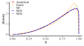
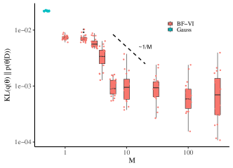
Figure 2: Upper panel: Comparison of the analytical posterior for the parameter $\pi$ in the Bernoulli model ${Y\sim\operatorname{Ber}(\pi)}$ with variational distributions achieved via Gaussian-VI and BF-VI with BP order $M=1,10,30$. Lower panel: Shows the dependence of the divergence $\operatorname{KL}(q_{\lambda}(w)\;\|\;p(w|D))$ on $M$ for 20 runs.

We now use BF-VI to approximate the posterior. To ensure that the modeled variational distribution to be restricted to the support of $\pi\in[0,1]$, we pipe the result of the flow through a sigmoid transformation. Fig. 2 shows the achieved variational distributions after minimizing the negative ELBO and demonstrates the robustness of BF-VI: When increasing the order $M$ of the BP, the resulting variational distribution gets closer to the posterior up to a certain value of $M$ and then does not deteriorate when further increasing $M$. The lower part of Fig. 2 indicates a convergence order of $M$ which can also be proven quite easily (see Appendix A). As expected, the Gaussian-VI has not enough flexibility to approximate the analytical posterior nicely (see Fig. 2).

Cauchy experiment

Here, we follow an example from [31] and fit an unconditional Cauchy model $Y\sim\text{Cauchy}(\xi,\gamma)$ to six samples which we have drawn from a mixture of two Cauchy distributions $Y\sim\text{Cauchy}(\xi_{1}=-2.5,\gamma=0.5)+\text{Cauchy}(\xi_{2}=2.5,\gamma=0.5)$. Due to the miss-specification of the model, the true posterior of the parameter $\xi$ has a bimodal shape which we have determined via MCMC (see Figure 3). We use BF-VI and Gaussian-VI to approximate the posterior of the Cauchy parameter $\xi$ by a variational distribution (as in [31] we assume that $\gamma=0.5$ is known). As in the Bernoulli experiment, also here BF-VI has enough flexibility to accurately approximate the bimodal posterior when $M$ is chosen large enough. Further increasing $M$ does not deteriorate the approximation. Gauss-VI fails as expected.

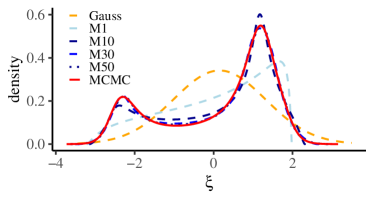
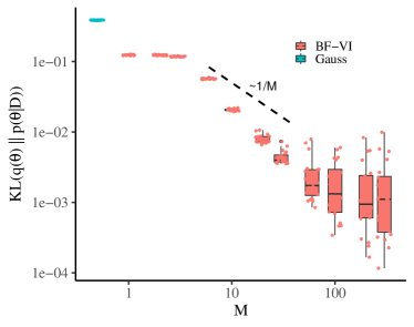
Figure 3: Upper panel: MCMC posterior distribution of the parameter $\xi$ in the miss-specified Cauchy model $Y\sim\text{Cauchy}(\xi,\gamma$) and the variational distributions estimated via Gaussian-VI or BF-VI ($M=1,20,30,50$). Lower panel: The divergence $\operatorname{KL}(q_{\lambda}(w)\;\|\;p(w|D))$ computed in 20 runs versus $M$.

IV-B Models with multiple parameters

The following experiments use BF-VI in multi-parameter Bayesian models and benchmark the achieved solutions versus MCMC or published state-of-the-art VI approximations (see table I). In the following experiments, we did not tune the flexibility of our BF-VI approach but allowed it to be quite high ($M=50$) since BF-VI does not suffer from being too flexible.

Toy linear regression experiment

To investigate, if dependencies between model parameters are correctly captured, we use here a simulated toy data set with two predictors and six data points to fit a Bayesian linear regression for modeling the conditional outcome distribution $(y|x_{1},x_{2})\sim\text{N}(\mu_{\bf{x}}=\mu_{0}+\beta_{1}x_{1}+\beta_{2}x_{2},\sigma)$.

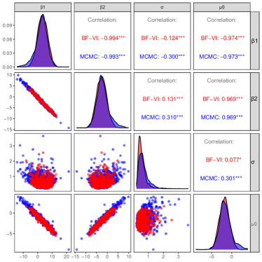
Figure 4: Toy linear regression posteriors. The model has four parameters: two regression coefficient $\beta_{1}$ and $\beta_{2}$, the intercept $\mu_{0}$, and the standard derivation $\sigma$. Samples from the true posterior resulting from MCMC (red) are overlayed with samples from the BF-VI approximation (blue).

Fig. 4 gives a visual impression of the joint true posterior of the four model parameters ($\mu_{0},\beta_{1},\beta_{2},\sigma$) determined via MCMC samples (blue) and its variational approximation (red) achieved via BF-VI. The strong correlation between the regression coefficients ($\beta_{1}$, $\beta_{2}$) of the two predictors is nicely captured by the BF-VI approximation. Further, the skewness of posterior marginals involving sigma is similar. However, we can clearly see, that BF-VI slightly underestimates the long tails of the posterior, confirming the known shortcoming of using the asymmetric KL-divergence in the objective function [3]. BF-VI ($\hat{k}=0.61$) outperforms MF-Gaussian-VI ($\hat{k}=1.34$), which can not (by construction) capture the dependencies (MF) or the non-Gaussian shapes (data not shown).

Diamond: Linear regression experiment

The Diamond benchmark for modeling the conditional outcome distribution $(y|\text{\boldmath$x$})\sim N(\mu_{x}=\mu_{0}+\text{\boldmath$x$}^{\top}\text{\boldmath$\beta$},\sigma)$ has 26 model parameters and 5000 data points (see [32] for reference MCMC samples and Stan code for a complete model definition). Since we have much more data than parameters, the posterior is expected to be a narrow Gaussian around the maximum-likelihood solution, which is indeed seen in the MCMC solution (see Fig. reffig:diamonds). In this setting BF-VI or NF-VI cannot profit from their ability to fit complex distributions. Still, [13] used this data set for bench-marking different VI methods, e.g. planar NF (PL-NF-VI), non-volume-preserving NF (NVP-NF-VI), and MF-Gaussian-VI. They achieved the best approximation via the simple Gaussian-VI ($\hat{k}=1.2$). The posterior approximation via PL-NF-VI and NVP-NF-VI have both been unsatisfactory ($\hat{k}=\infty$). We use the same amount of sampling ($S=10$), and achieved with BF-VI a better approximation of the posterior $\hat{k}=30.23$ but is still inferior to the Gaussian-VI (see Fig. reffig:diamonds).

8schools: Hierarchical model experiment

The 8schools data set is a benchmark data set for fitting a Bayesian hierarchical normal model and is known to be challenging for VI approaches [30], [33]. It has 8 data points, corresponding to eight schools, which have conducted independent coaching programs to enhance the SAT (Scholastic Assessment Test) score of their students. There are two commonly used parameterizations, centered parameterization (CP) and non-centered parameterization (NCP), see Table I for more details of these parametrizations and [32] for complete model definitions in Stan. In both parametrizations, the model has 10 parameters. In [13] this benchmark data set was fitted with two NF-based methods and MF-Gaussian-VI. For the CP version [13] reported $\hat{k}_{\text{CP}}=1.3,1.1,0.9$ for PL-NF-VI, NVP-NF-VI, MF-Gaussian-VI, which are all outperformed by our BF-VI method with $\hat{k}_{\text{CP}}=0.61$. For the NCP version [13] reported $\hat{k}_{\text{NCP}}=1.2,0.7,0.7$ (same order), and again BF-VI yields a superior $\hat{k}_{\text{NCP}}=0.35$. A visual inspection of the true MCMC posterior and its variational approximation showed again the issue of the underestimated distribution tails (see Fig. S3).

NN based non-linear regression experiment

For this experiment, we use a small Bayesian NN for non-linear regression fitted on 9 data points. The model for the conditional outcome distribution is $(y|\text{\boldmath$x$})\sim N(\mu(\text{\boldmath$x$}),\sigma)$. The small size of the used BNN with only one hidden layer comprising 3 neurons and one neuron in the output layer giving $\mu(\text{\boldmath$x$})$, allows us to determine the posterior via MCMC.

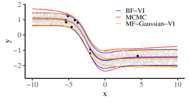
Figure 5: Posterior predictive distribution of non-linear regression model $(y|\text{\boldmath$x$})\sim N(\mu(\text{\boldmath$x$}),\sigma)$ where the conditional mean is modeled by a BNN using MCMC, MF-Gaussian-VI, or BF-FI.

We then use BF-VI, and MF-Gaussian-VI to fit this BNN. Because the weights in a BNN with hidden layers are not directly interpretable, they are not of direct interest and therefore the fit of a BNN is commonly assessed on the level of the posterior predictive distribution (see Figure 5). In this example, the more flexible BF-VI only yields a small improvement in approximating the true posterior predictive distribution when compared to the more easy approach with MF-Gaussian-VI.

Melanoma : Semi-structured NN experiment

In this experiment we use BF-VI for semi-structured models (see Fig. 6) where complex data like images can be modeled by deep NN together with interpretable model components. Because of the involved deep NN model components, MCMC is not anymore feasible. As dataset we use the SIIM-ISIC Melanoma Classification Challenge data. The data comes from 33126 patients (6626 as test set, 21200+5300 as train plus validation set) with confirmed diagnosis of their skin lesions which is in $\approx 98$% benign ($y=0$) and in $\approx 2$% malignant ($y=1$). The provided data $D=(B,x)$ is semi-structured since it comprises (unstructured) image data $B$ from the patient’s lesion along with (structured) tabular data $x$, i.e. the patient’s age.

We fit the conditional outcome distribution $(y|D)\sim\operatorname{Ber}\big{(}\pi_{D})$ by modeling the probability for a lesion to be malignant $\pi_{D}=p(y=1|D)=\sigma(h)$ using the sigmoid function. We study three models for h depending on $B$ and/or $x$:

M1 (DL-Model) $h=\mu(B)$: As baseline we use a deep convolutional neural network (CNN) based on the melanoma image data (see Fig. 6 c)) with a total of 419,489 parameters to take advantage of the predictive power of DL on complex image data. For this DL model, we use deep ensembling [34] by fitting three CNN models with different random initialization and averaging the predicted probabilities. The achieved test performance and its comparison to other models is discussed in the last paragraph of this section.

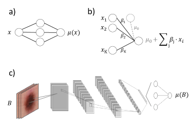
Figure 6: The architecture of the used NN models or model parts. a) Dense NN with one hidden layer to model non-linear dependencies from the input. b) Dense NN without hidden layer to model linear dependencies from tabular input data. c) CNN to model non-linear dependencies from the image input.

M2 (Logistic Regression) $h=\mu_{0}+\beta_{1}\cdot x$: When using tabular features $x$, interpretable models can be built. We consider a Bayesian logistic regression with age as the only explanatory variable $x$ and use a BNN without a hidden layer to set up the model (see Figure 6 b with only one input feature $x$). In logistic regression a latent variable is modeled by a linear predictor $h=\mu_{0}+\beta_{1}\cdot x$ which determines the probability for a lesion to be malignant via $\pi_{x}=\sigma\big{(}\mu_{0}+\beta_{1}\cdot x\big{)}$ allowing to interpret $e^{\beta_{1}}$ as the odds-ratio, i.e. the factor by which the odds for a lesions to be malignant changes when increasing the predictor $x$ by one unit. In Figure 7, we compare the exact MCMC posterior of $\beta_{1}$ with the BF-VI approximation demonstrating that BF-VI accurately approximates the posterior.

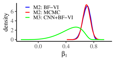
Figure 7: Posteriors for the age-effect parameter $\beta_{1}$ in the Melanoma models M2 and M3.

M3 (semi-structured) $h=\mu_{0}(B)+\beta_{1}\cdot x$: This model integrates image and tabular data and combines the predictive power of M1 with the interpretability of M2. We use a (non-Bayesian) CNN that determines $\mu_{0}(B)$ and BF-VI for the NN without hidden layer that determines $\beta_{1}$ (see Figure 6 b and c). Both NNs are jointly trained by optimizing the ELBO. The resulting posterior for $\beta_{1}$ differs from the simple logistic regression (see Figure 7) indicating a smaller age effect after including the the image. Again, $e^{\beta_{1}}$ can be interpreted as the factor by which the odds for a lesion to be malignant changes when increasing the predictor age by one unit and holding the image constant.

While the main interest of our study is on the posteriors, we also determine the predictive performance on the testset. To quantify and compare the test prediction performances we look at the achieved log-scores (M1:-0.078, M2:-0.085, M3: -0.076) and the AUCs with 95$\%$ CI (M1:$0.81(0.78,0.84)$, M2:$0.66(0.61,0.71)$, M3: $0.82(0.79,0.85)$). For both measures higher is better. It is interesting to note that the image based models (M1, M3) have higher predictive power than M2 which only uses the tabular data. The semi-structured model M3, including both tabular and image information, has higher predictive power than the CNN (M1), which only uses images, and, in addition, provides interpretable parameters for the tabular data along with uncertainty quantification.

V Summary and outlook

The proposed BF-VI is flexible enough to approximate any posterior in principle, without being restricted to known parametric variational distributions like Gaussians. In benchmark experiments, BF-VI accurately fits non-trivial posteriors in low dimensional problems. For higher dimensional models, BF-VI outperforms other NF-VI methods [13] on the studied benchmark data sets. Still, we observe that the posterior can not be fitted perfectly in high dimensions by BF-VI, especially the tails of the approximation are too short. We attribute this limitation to known difficulties in the optimization process and the asymmetry of the KL divergence. These challenges of VI, were not in the focus of our study, and we leave it to further research.

To the best of our knowledge we are the first who demonstrated how VI can be used in semi-structured models. We used BF-VI on the public melanoma challenge data set integrating image data and tabular data by combining a deep CNN and an interpretable model part. We see the main application of BF-VI in models with interpretable parameters i.e., statistical models or semi-structured models and less in black-box DL. Especially in semi-structured models with deep NN components, that cannot be fitted with MCMC, BF-VI allows to determine variational distribution for the interpretable model parts. Moreover, efficient SGD optimizers for jointly fitting all model parts can be used in BF-VI. We plan to extend our research on BF-VI for semi-structured models in the future and investigate the quality of the posterior approximations.

VI Acknowledgements

Part of the work has been founded by the Federal Ministry of Education and Research of Germany (BMBF) in the project DeepDoubt (grant no. 01IS19083A). We further would like to thank Lucas Kook, Rebekka Axthelm, and Nadja Klein for fruitful discussions.

Appendix

A Tightness of Variational Bound in the limit $M\rightarrow\infty$,

In the following we show for the one dimensional case that for a transformation function build from Bernstein polynomials of order $M$ there exists a solution so that $\operatorname{KL}(q_{\lambda,M}(\theta)\;\|\;p(\theta|D))$ in (2) asymptotically vanishes with $1/M$.

We assume that the posterior $p(\theta|D)$ is continuous in the compact interval $[\theta_{a},\theta_{b}]$ with CDF $F_{\theta}(\theta)$ and that the first three derivatives of $F_{\theta}(\theta)$ exists. Without loss of generality, we set $\theta_{a}=0$ and $\theta_{b}=1$. This allows us to construct a transformation $h:\theta\rightarrow Z$ transforming between $\theta$ with CDF $F_{\theta}$ and a random variable $Z$ with CDF $F_{Z}$ by requiring $F_{Z}(h(\theta))=F_{\theta}(\theta)$ via

$$h(\theta)=F_{Z}^{-1}(F_{\theta}(\theta)).$$ (S1)

We assume that $F_{Z}$ has continuous derivatives up through order 3, then from (S1) it follows that $h(\theta)$ has continuous derivatives up to order 3. Further, we require that the number of roots of $h^{\prime\prime}(\theta)$ and $h^{\prime\prime\prime}(\theta)$ are countable. In addition, we require that the density $p_{Z}(z)>0$. We approximate the posterior density $p(\theta|D)$ by $q_{\lambda}(\theta)$ by approximating $h(\theta)$ with a Bernstein polynomial of order $M$ given by:

$$B_{M}(\theta)=\sum_{m=0}^{M}h\left(\frac{m}{M}\right)\binom{M}{m}\;\theta^{m}(1-\theta)^{M-n}$$ (S2)

Note that we fixed the coefficients of the transformation here. This is valid since we just want to prove that a particular solution exists for that (2) asymptotically vanishes with $1/M$. As shown in [26] the Bernstein approximation ”is at least as smooth” as $h(\theta)$, in our case that at least the first 3 derivatives of $B_{M}(\theta)$ exists and converge to the corresponding derivatives of $h(\theta)$. In a first step, we upper bound the KL-divergence, to that part of $\theta^{\prime}\subset\theta$ where $\log(\frac{q_{\lambda}(\theta)}{p(\theta|D)})>0$ since $q_{\lambda}(\theta)\geq 0$, the following approximation hold

$$\operatorname{KL}(q_{\lambda}(\theta)\;\|\;p(\theta|D))=\int_{0}^{1}q_{\lambda}(\theta)\log\left(\frac{q_{\lambda}(\theta)}{p(\theta|D)}\right)\;d\theta\leq\int_{\theta^{\prime}}q_{\lambda}(\theta)\log\left(\frac{q_{\lambda}(\theta)}{p(\theta|D)}\right)\;d\theta$$ (S3)

Using the change of variable formula, we can express the densities of the posterior as $p(\theta|D)=p_{Z}\left(h(\theta)\right)\cdot|h^{\prime}(\theta)|$ and its approximation as $q_{\lambda}(\theta)=p_{Z}\left(B_{M}(\theta)\right)\cdot|B^{\prime}_{M}(\theta)|$, the dash indicates a derivative w.r.t. $\theta$. Hence the KL-Divergence is bounded by:

$$\operatorname{KL}(q_{\lambda}(\theta)\;\|\;p(\theta|D))\leq\int_{\theta^{\prime}}q_{\lambda}(\theta)\log\left(\frac{p_{Z}\left(B_{M}(\theta)\right)\cdot|B^{\prime}_{M}(\theta)|}{p_{Z}\left(h(\theta)\right)\cdot|h^{\prime}(\theta)|}\right)\;d\theta$$ (S4)

The transformation function $h(\theta)$ is either strictly monotonic increasing or decreasing, w.l.o.g. we assume that $h^{\prime}(\theta)>0$. This leads to ordered coefficients $h(m/M)$ and so $B^{\prime}_{M}(\theta)>0$.

Since the density $p_{Z}(z)$ and the derivative $B^{\prime}_{M}(\theta)$ of Bernstein approximation are finite, so is $q_{\lambda}(\theta)=p_{Z}\left(B_{M}(\theta)\right)\cdot|B^{\prime}_{M}(\theta)|$. This allows to upper bound the integral in (S4) with $C=\sup(q_{\lambda}(\theta))$ in the range $\theta\in[0,1]$ by:

$$\operatorname{KL}(q_{\lambda}(\theta)\;\|\;p(\theta|D))\leq C\cdot\underbrace{\int_{\theta^{\prime}}\log\left(\frac{p_{Z}\left(B_{M}(\theta)\right)}{p_{Z}\left(h(\theta)\right)}\right)\;d\theta}_{=:I_{1}}+C\cdot\underbrace{\int_{\theta^{\prime}}\log\left(\frac{B^{\prime}_{M}(\theta)}{h^{\prime}(\theta)}\right)\;d\theta}_{=:I_{2}}$$ (S5)

With increasing $M$ the term $\Delta=B_{M}(\theta)-h(\theta)$ gets arbitrarily small. We do a Taylor expansion $p_{Z}(B_{M}(\theta))=p_{Z}(h(\theta)+\Delta)=p_{Z}(h(\theta))+p^{\prime}_{Z}(h(\theta))\Delta+\mathcal{O}(\Delta^{2})$. With $\log(1+x)\leq x$ the first integral $I_{1}$ can be approximated as

$$I_{1}=\int_{\theta^{\prime}}\log\left(1+\frac{p_{Z}^{\prime}\left(h(\theta)\right)}{p_{Z}\left(h(\theta)\right)}\Delta+\mathcal{O}(\Delta^{2})\right)\;d\theta\leq\int_{\theta^{\prime}}\left(\frac{p_{Z}^{\prime}\left(h(\theta)\right)}{p_{Z}\left(h(\theta)\right)}\Delta+\mathcal{O}(\Delta^{2})\right)\;d\theta$$ (S6)

Since $p_{Z}(z)>0$ we can set $C_{2}=\sup(\frac{p_{Z}^{\prime}\left(h(\theta)\right)}{p_{Z}\left(h(\theta)\right)})$ yielding:

$$I_{1}\leq C_{2}\cdot\int_{\theta^{\prime}}\left(B_{M}(\theta)-h(\theta)\right)\;d\theta+\mathcal{O}(\Delta^{2})$$ (S7)

The Voronovskaya theorem (see [26]) states that $B_{M}(\theta)-h=\theta/(2M)h^{\prime\prime}(\theta)+o(M^{-1})$ for $h^{\prime\prime}(\theta)\neq 0$. Assuming that $h^{\prime\prime}(\theta)=0$ only on a countable set of points, the asymptotic of $I_{1}$ is given by $1/M$.

Using $\log(x)\leq x-1$ the second integral can be bounded as follows.

$$I_{2}=\int_{\theta^{\prime}}\log\left(\frac{B^{\prime}_{M}(\theta)}{h^{\prime}(\theta)}\right)\;d\theta\leq\int_{\theta^{\prime}}\left(\frac{B^{\prime}_{M}(\theta)}{h^{\prime}(\theta)}-1\right)\;d\theta=\int_{\theta^{\prime}}\frac{1}{h^{\prime}(\theta)}\left(B^{\prime}_{M}(\theta)-h^{\prime}(\theta)\right)\;d\theta$$ (S8)

According to our assumptions $h^{\prime}(\theta)>0$ and so the supremum $C_{3}=\sup(1/h^{\prime}(\theta))$ exists.

$$I_{2}\leq C_{3}\int_{\theta^{\prime}}\left(B^{\prime}_{M}(\theta)-h^{\prime}(\theta)\right)\;d\theta\leq\frac{1}{M}\int_{\theta^{\prime}}\left(\theta/2h^{\prime\prime\prime}(\theta)+1/2h^{\prime\prime}(\theta)+o(M^{-1})\right)\;d\theta$$ (S9)

This shows that the KL-Divergence in (2) asymptotically converges to zero as $1/M$.

B Experimental details of and additional results

In the following, we give additional details for the experiments.

B-A Bernoulli Example

B-A1 The data generative process

Two samples are drawn from a Bernoulli distribution.

B-A2 The actual data

The realizations are $y_{1}=1$ and $y_{2}=2$.

B-A3 Details of the training procedure

To demonstrate the possibility that the described solution converges in principal to the exact solution, we used a rather large number of MC-samples $S=1000$ and epochs=1000 for the training.

B-A4 Additional Results (tightness of the ELBO)

For this example we can estimate the KL-divergence via

$$\operatorname{KL}(q_{\lambda}(\theta)\;\|\;p(\theta|D))=\int~{}q_{\lambda}(\theta)\log\left(\frac{q_{\lambda}(\theta)}{p(\theta|D)}\right)d\theta\\ \approx\frac{1}{S}\sum_{s\sim q_{\lambda}}\log\left(\frac{q_{\lambda}(\theta_{s})}{p(\theta_{s}|D)}\right)$$ (S10)

The sum is calculated from the samples $\theta_{s}$ of the trained approximative distribution, which can be obtained via the trained transformation function. The likelihood $p(D|\theta_{s})$ and prior $p(\theta_{s})$ for those samples can be easily calculated and probabilities $q_{\lambda}(\theta_{s})$ can be calculated via (5). In this simple case the posterior can be calculated analytically to $p(\theta_{s}|D)=\operatorname{Be}_{(\alpha+\sum{y_{i}},\beta+n-\sum{y_{i}})}(\theta_{s})=\operatorname{Be}_{(3.1,1.1)}(\theta_{s})$.

In Figure 2 we show a direct comparison of posterior and its approximation the dependence of the tightness of the ELBO on $M$ in the lower part is calculated via (S10). At a $M\approx 10$ the KL reaches a minimum, corresponding to an accurate approximation of the posterior. Further increasing $M$ does not decrease the error any further, which we attribute to the SGD approximation. More importantly increasing $M$ and thus the flexibility does not deteriorate the approximation.

B-B Chauchy Example

B-B1 The data generative process

Six samples are drawn from a mixture of two Cauchy distributions $y\sim\text{Cauchy}(\xi_{1}=-2.5,\gamma=0.5)+\text{Cauchy}(\xi_{2}=2.5,\gamma=0.5)$.

B-B2 The actual data

From the data generating process, we draw the following 6 examples $y=1.2083935,-2.7329216,4.1769943,1.9710574,-4.2004027,-2.384988$.

B-B3 Details of the Model

We use an unconditional Cauchy model $y\sim\text{Cauchy}(\xi,\gamma=0.5)$ were $\gamma=0.5$ is given. Note that this model is misspecified and give rise to a multimodal posterior. The Stan code is given in Listing (1)

B-B4 Details of the training procedure

To demonstrate the possibility that the described solution converges in principal to the exact solution, we used a rather large number of MC-samples $S=10000$ and epochs=1000 for the training.

B-B5 Additional Results (tightness of the ELBO)

For this example, we cannot determine the posterior $p(\theta_{s}|D)=\frac{p(D|\theta_{s})p(\theta_{s})}{\int p(D|\theta_{s})p(\theta_{s})\;d\theta}$ analytically anymore. However, we can rewrite (S10) to:

$$\operatorname{KL}(q_{\lambda}(\theta)\;\|\;p(\theta|D))\approx\frac{1}{S}\sum_{s\sim q_{\lambda}}\log\left(\frac{q_{\lambda}(\theta_{s})}{p(\theta_{s}|D)}\right)=\frac{1}{S}\sum_{s\sim q_{\lambda}}\log\left(\frac{q_{\lambda}(\theta_{s})}{p(D|\theta_{s})p(\theta_{s})}\right)+\underbrace{\log\left(\int p(D|\theta)p(\theta)d\theta\right)}_{=\log(P(D))}$$ (S11)

For this examples the log-evidence $\log(P(D))=-21.43069$ is obtained by numerical integration.

In Figure 3 we show a direct comparison of posteriors the dependence of the tightness of the ELBO on $M$ calculated in the lower part is calculated via (S11).

B-C Toy linear regression example

In this example a posterior is generated, which displays a strong correlation between the results.

B-C1 The data generative process

The data is generated by the following R-code.

⬇

set.seed(42)

N = 6L # number data points

P = 2L #number of predictors

z_dg = rnorm(N, mean=0, sd=1)

x_dg = scale(rnorm(N, mean = 1.42*z_dg, sd = 0.1), scale = FALSE)

y_r = rnorm(N, mean = 0.42*x_dg - 1.1 * z_dg, sd=0.42)

B-C2 The actual data

⬇

> x_r

[,1] [,2]

[1,] 1.3709584 1.48475156

[2,] -0.5646982 -1.42449894

[3,] 0.3631284 0.10432308

[4,] 0.6328626 0.27923186

[5,] 0.4042683 0.09138635

[6,] -0.1061245 -0.53519391

> y_r

[1] -1.46778013 -0.09421285 -0.41162052 -0.31177232 -0.52569912 -1.22375575

B-C3 Details of the Model

The Stan code is given in Listing (2)

B-C4 Details of the training procedure

The model has been trained with $M=10$, 15000 epochs and $S=600$.

B-C5 Additional Results

Figure S1 show the result for MF-Gaussian approximation. As is visible the mean field approach cannot capture the multivariate correlation of the posterior, and strongly focus on the mode of the posterior.

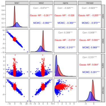
Figure S1: Mean-Field Gaussian result for the linear regression posteriors.

B-D Diamond

B-D1 Details of the Model

The Stan code can be found in the Listing 3.

B-D2 Details of the training procedure

In order to be comparable with [Dhaka et al., 2021], we used 30000 epochs, S = 10 and M = 50.

B-D3 Additional Results

In Figure S2 we show samples from the marginals of the MCMC solution and the BF-VI approximation. This dataset is quite challenging, we did not get satisfactory MCMC samples and took the reference posterior samples from the posteriorDB.

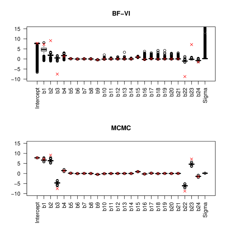
Figure S2: Comparison of samples from the marginals of MCMC samples and samples from the approximative posterior for the diamond data set. Here the MCMC solution is very narrow and the BF-VI (as other approximations) fails to converge to the narrow posterior. The red crosses indicates the maximum likelihood solution.

B-E 8School

The 8-Schools examples comes in NCP (defined in Listing (4) and CP paramerizations (see Listing (5).

B-E1 Details of the training procedure

In order to be comparable with [13] we used 15000 epochs, $S=10$ and $M=50$.

B-E2 Additional Results

In Figure S3 we show samples from the marginals of the 8 dimensional parameter $\theta$ (right side, centered parameterization) and $\tilde{\theta}$ (left side, non-centered) parameterization. For the MCMC samples the easier centered parameterization yielding $\tilde{\theta}$ is used for both cases and $\theta$ is calculated from it. We see a underestimation of the true posterior.

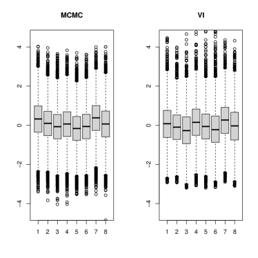
Figure S3: Marginal samples from MCMC and BF-VI for the 8 schools examples. For the NCP-parametrization $\tilde{\theta}_{i}$ ($i=1,\ldots,8$) is shown on left two plots and $\theta$ right two plots (CP-Parametrization).

B-F NN based non-linear regression example

B-F1 The actual data

We have $N=9$ samples with
$x=-5.412390,-4.142973,-5.100401,-4.588446,-2.057037,-2.003591,-3.740448,-5.344997,4.506781$ and
$y=0.9731220,0.9664410,1.2311585,0.5193988,-1.2059958,-0.9434611,0.8041748,0.8299642,-1.3704962$.

B-F2 Details of the Model

The model is a simple NN with one hidden layer comprising 3 neurons and one neuron in the output layer giving the conditional mean. All weights have a $N(0,1)$ prior. The complete Stan code is given in Listing 6.

B-F3 Details of the training procedure

For BF-VI the there has been trained for 20’000 epochs with $M=50$ and $S=600$ using RMSProb.

B-G Stan code

To unambiguously define the models, we provide the Stan code in the following.

Listing 1: ”Stan code for the Chauchy example”

⬇

data{

int<lower=0> N;

real<lower=0> gamma;

vector[N] y;

}

parameters{

real xi;

}

model{

y ~ cauchy(xi, gamma);

xi ~ normal(0, 1);

}

Listing 2: ”Stan code for the toy linear regression example”

⬇

data {

int<lower=0> N;

int<lower=1> P;

vector[N] y;

matrix[N,P] x;

}

parameters {

vector[P] w;

real b;

real<lower=0> sigma;

}

model {

y ~ normal(x * w + b, sigma);

b ~ normal(0,10);

w ~ normal(0, 10);

sigma ~ lognormal(0.5,1);

}

Listing 3: ”Stan code for the Diamond Example”

⬇

// The code has been taken from https://github.com/stan-dev/posteriordb

// generated with brms 2.10.0

functions {

}

data {

int<lower=1> N; // number of observations

vector[N] Y; // response variable

int<lower=1> K; // number of population-level effects

matrix[N, K] X; // population-level design matrix

int prior_only; // should the likelihood be ignored?

}

transformed data {

int Kc = K - 1;

matrix[N, Kc] Xc; // centered version of X without an intercept

vector[Kc] means_X; // column means of X before centering

for (i in 2:K) {

means_X[i - 1] = mean(X[, i]);

Xc[, i - 1] = X[, i] - means_X[i - 1];

}

}

parameters {

vector[Kc] b; // population-level effects

// temporary intercept for centered predictors

real Intercept;

real<lower=0> sigma; // residual SD

}

transformed parameters {

}

model {

// priors including all constants

target += normal_lpdf(b | 0, 1);

target += student_t_lpdf(Intercept | 3, 8, 10);

target += student_t_lpdf(sigma | 3, 0, 10)

- 1 * student_t_lccdf(0 | 3, 0, 10);

// likelihood including all constants

if (!prior_only) {

target += normal_id_glm_lpdf(Y | Xc, Intercept, b, sigma);

}

}

generated quantities {

// actual population-level intercept

real b_Intercept = Intercept - dot_product(means_X, b);

}

Listing 4: ”Stan code for 8 Schools in the NCP parameterization”

⬇

//eight_schools_ncp.stan

data {

int<lower=0> J;

real y[J];

real<lower=0> sigma[J];

}

parameters {

real mu;

real<lower=0> tau;

real theta_tilde[J];

}

transformed parameters {

real theta[J];

for (j in 1:J)

theta[j] = mu + tau * theta_tilde[j]; //theta[j] ~ N(mu, tau*theta_tilde[j])

}

model {

mu ~ normal(0, 5);

tau ~ cauchy(0, 5);

theta_tilde ~ normal(0, 1);

y ~ normal(theta, sigma);

}

Listing 5: ”Stan code for the 8 schools example in the CP parametrization”

⬇

//eight_schools_cp.stan

data {

int<lower=0> J;

real y[J];

real<lower=0> sigma[J];

}

parameters {

real mu;

real<lower=0> tau;

real theta[J];

}

model {

//Priors for p(mu, tau, theta)

mu ~ normal(0, 5);

tau ~ cauchy(0, 5);

theta ~ normal(mu, tau);

//Likelihood

y ~ normal(theta, sigma);

}

Listing 6: ”Stan code for the NN based non-linear regression example”

⬇

functions {

vector calculate_mu(matrix X, matrix bias_first_m,

real bias_output, matrix w_first, vector w_output, int num_layers) {

int N = rows(X);

int num_nodes = rows(w_first);

matrix[N, num_nodes] layer_values[num_layers - 2];

vector[N] mu;

layer_values[1] = inv_logit(bias_first_m + X * w_first’);

mu = bias_output + layer_values[num_layers - 2] * w_output;

return mu;

}

}

data {

int<lower=0> N; // num data

int<lower=0> d; // dim x

int<lower=0> num_nodes; // num hidden unites

int<lower=1> num_middle_layers; // num hidden layer

matrix[N,d] X; // X

real y[N]; // y

int<lower=0> Nt; // num predicive data

matrix[Nt,d] Xt; // X predicive

real<lower=0> sigma; // const sigma

}

transformed data {

int num_layers;

num_layers = num_middle_layers + 2;

}

parameters {

vector[num_nodes] bias_first;

real bias_output;

matrix[num_nodes, d] w_first;

vector[num_nodes] w_output;

// hyperparameters

real<lower=0> bias_first_h;

real<lower=0> w_first_h;

real<lower=0> w_output_h;

}

transformed parameters {

matrix[N, num_nodes] bias_first_m = rep_matrix(bias_first’, N);

}

model{

vector[N] mu;

mu = calculate_mu(X, bias_first_m, bias_output, w_first, w_output, num_layers);

y ~ normal(mu,sigma);

//priors

bias_first_h ~ normal(0, 1);

bias_first ~ normal(0, 1);

bias_output ~ normal(0, 1);

w_first_h ~ normal(0, 1);

to_vector(w_first) ~ normal(0, 1);

w_output_h ~ normal(0, 1);

w_output ~ normal(0, 1);

}

generated quantities{

vector[Nt] predictions;

matrix[Nt, num_nodes] bias_first_mg = rep_matrix(bias_first’, Nt);

vector[Nt] mu;

mu = calculate_mu(Xt, bias_first_mg, bias_output,w_first, w_output, num_layers);

for(i in 1:Nt){

predictions[i] = normal_rng(mu[i],sigma);

}

}

References

- [1] M. I. Jordan, Z. Ghahramani, T. S. Jaakkola, and L. K. Saul, “An introduction to variational methods for graphical models,” Machine learning, vol. 37, no. 2, pp. 183–233, 1999.
- [2] M. J. Wainwright and M. I. Jordan, Graphical models, exponential families, and variational inference. Now Publishers Inc, 2008.
- [3] D. M. Blei, A. Kucukelbir, and J. D. McAuliffe, “Variational inference: A review for statisticians,” Journal of the American statistical Association, vol. 112, no. 518, pp. 859–877, 2017.
- [4] A. K. Dhaka, A. Catalina, M. R. Andersen, M. Magnusson, J. H. Huggins, and A. Vehtari, “Robust, accurate stochastic optimization for variational inference,” arXiv preprint arXiv:2009.00666, 2020.
- [5] D. Blei, R. Ranganath, and S. Mohamed, “Variational inference: Foundations and modern methods,” NIPS Tutorial, 2016.
- [6] R. Ranganath, S. Gerrish, and D. Blei, “Black box variational inference,” in Artificial intelligence and statistics. PMLR, 2014, pp. 814–822.
- [7] S. Farquhar, L. Smith, and Y. Gal, “Liberty or depth: Deep bayesian neural nets do not need complex weight posterior approximations,” arXiv preprint arXiv:2002.03704, 2020.
- [8] D. Rezende and S. Mohamed, “Variational inference with normalizing flows,” in International Conference on Machine Learning. PMLR, 2015, pp. 1530–1538.
- [9] I. Kobyzev, S. Prince, and M. Brubaker, “Normalizing flows: An introduction and review of current methods,” IEEE Transactions on Pattern Analysis and Machine Intelligence, 2020.
- [10] D. P. Kingma and P. Dhariwal, “Glow: generative flow with invertible 1 1 convolutions,” in Proceedings of the 32nd International Conference on Neural Information Processing Systems, 2018, pp. 10 236–10 245.
- [11] A. v. d. Oord, S. Dieleman, H. Zen, K. Simonyan, O. Vinyals, A. Graves, N. Kalchbrenner, A. Senior, and K. Kavukcuoglu, “Wavenet: A generative model for raw audio,” arXiv preprint arXiv:1609.03499, 2016.
- [12] C. Louizos and M. Welling, “Multiplicative normalizing flows for variational bayesian neural networks,” in International Conference on Machine Learning. PMLR, 2017, pp. 2218–2227.
- [13] A. K. Dhaka, A. Catalina, M. Welandawe, M. R. Andersen, J. Huggins, and A. Vehtari, “Challenges and opportunities in high-dimensional variational inference,” arXiv preprint arXiv:2103.01085, 2021.
- [14] P. Jaini, K. A. Selby, and Y. Yu, “Sum-of-squares polynomial flow,” in International Conference on Machine Learning. PMLR, 2019, pp. 3009–3018.
- [15] C. Durkan, A. Bekasov, I. Murray, and G. Papamakarios, “Neural spline flows,” Advances in Neural Information Processing Systems, vol. 32, pp. 7511–7522, 2019.
- [16] T. Hothorn, T. Kneib, and P. Bühlmann, “Conditional transformation models,” Journal of the Royal Statistical Society: Series B: Statistical Methodology, pp. 3–27, 2014.
- [17] T. Hothorn, L. Moest, and P. Buehlmann, “Most likely transformations,” Scandinavian Journal of Statistics, vol. 45, no. 1, pp. 110–134, 2018.
- [18] L. Kook, L. Herzog, T. Hothorn, O. Dürr, and B. Sick, “Deep and interpretable regression models for ordinal outcomes,” arXiv preprint arXiv:2010.08376, 2020.
- [19] S. Bernšteın, “Démonstration du théoreme de weierstrass fondée sur le calcul des probabilities,” Comm. Soc. Math. Kharkov, vol. 13, pp. 1–2, 1912.
- [20] M. Buri, A. Curt, J. Steeves, and T. Hothorn, “Baseline-adjusted proportional odds models for the quantification of treatment effects in trials with ordinal sum score outcomes,” BMC medical research methodology, vol. 20, pp. 1–14, 2020.
- [21] B. Sick, T. Hathorn, and O. Dürr, “Deep transformation models: Tackling complex regression problems with neural network based transformation models,” in 2020 25th International Conference on Pattern Recognition (ICPR). IEEE, 2021, pp. 2476–2481.
- [22] N. Klein, T. Hothorn, L. Barbanti, and T. Kneib, “Multivariate conditional transformation models,” Scandinavian Journal of Statistics, 2019.
- [23] P. F. Baumann, T. Hothorn, and D. Rügamer, “Deep conditional transformation models,” arXiv preprint arXiv:2010.07860, 2020.
- [24] M. Carlan, T. Kneib, and N. Klein, “Bayesian conditional transformation models,” arXiv preprint arXiv:2012.11016, 2020.
- [25] S. Ramasinghe, K. Fernando, S. Khan, and N. Barnes, “Robust normalizing flows using bernstein-type polynomials,” arXiv preprint arXiv:2102.03509, 2021.
- [26] R. T. Farouki, “The bernstein polynomial basis: A centennial retrospective,” Computer Aided Geometric Design, vol. 29, no. 6, pp. 379–419, 2012.
- [27] G. Papamakarios, T. Pavlakou, and I. Murray, “Masked autoregressive flow for density estimation,” in Proceedings of the 31st International Conference on Neural Information Processing Systems, 2017, pp. 2335–2344.
- [28] V. I. Bogachev, A. V. Kolesnikov, and K. V. Medvedev, “Triangular transformations of measures,” Sbornik: Mathematics, vol. 196, no. 3, p. 309, 2005.
- [29] C. Blundell, J. Cornebise, K. Kavukcuoglu, and D. Wierstra, “Weight uncertainty in neural network,” in International Conference on Machine Learning. PMLR, 2015, pp. 1613–1622.
- [30] Y. Yao, A. Vehtari, D. Simpson, and A. Gelman, “Yes, but did it work?: Evaluating variational inference,” in International Conference on Machine Learning. PMLR, 2018, pp. 5581–5590.
- [31] Y. Yao, A. Vehtari, and A. Gelman, “Stacking for non-mixing bayesian computations: The curse and blessing of multimodal posteriors,” arXiv preprint arXiv:2006.12335, 2020.
- [32] M. Magnusson, P. Bürkner, and A. Vehtari, “posteriordb: a set of posteriors for Bayesian inference and probabilistic programming,” 9 2021.
- [33] J. Huggins, M. Kasprzak, T. Campbell, and T. Broderick, “Validated variational inference via practical posterior error bounds,” in International Conference on Artificial Intelligence and Statistics. PMLR, 2020, pp. 1792–1802.
- [34] B. Lakshminarayanan, A. Pritzel, and C. Blundell, “Simple and scalable predictive uncertainty estimation using deep ensembles,” arXiv preprint arXiv:1612.01474, 2016.