Numerical-relativity validation of effective-one-body waveforms
in the intermediate-mass-ratio regime

Abstract

One of the open problems in developing binary black hole (BBH) waveforms for gravitational wave astronomy is to model the intermediate mass ratio regime and connect it to the extreme mass ratio regime. A natural approach is to employ the effective one body (EOB) approach to the two-body dynamics that, by design, can cover the entire mass ratio range and naturally incorporates the extreme mass ratio limit. Here we use recently obtained numerical relativity (NR) data with mass ratios $m_{1}/m_{2}=(7,15,\,32,\,64,\,128)$ to test the accuracy of the state-of-the-art EOB model TEOBResumS in the intermediate mass ratio regime. We generally find an excellent EOB/NR consistency around merger and ringdown for all mass ratios and for all available subdominant multipoles, except for the $\ell=m=5$ one. This mode can be crucially improved using the new large-mass ratio NR data of this paper. The EOB/NR inspirals are also consistent with the estimated NR uncertainties. We also use several NR datasets taken by different public catalogs to probe the universal behavior of the multipolar hierarchy of waveform amplitudes at merger, that smoothly connects the equal-mass BBH to the test-mass result. Interestingly, the universal behavior is strengthened if the nonoscillatory memory contribution is included in the NR waveform. Future NR simulations with improved accuracy will be necessary to further probe, and possibly quantitatively refine, the TEOBResumS transition from late inspiral to plunge in the intermediate mass ratio regime.

I Introduction

While ground based gravitational wave detectors like LIGO-Virgo Abbott et al. (2019); Vir are particularly sensitive to comparable (stellar) mass binaries, third generation (3G) ground detectors Pürrer and Haster (2020) and space detectors, like LISA, will also be sensitive to the observation of very unequal mass binary black holes Gair et al. (2017). These will allow the search and study of intermediate mass black holes, either as the large hole in a merger with a stellar mass black hole (a source for 3G detectors) or as the smaller hole in a merger with a supermassive black hole (a source for LISA).

LISA will be sensitive to the inspiral and merger of black-hole systems where the primary is significantly (10-1000 times) larger than the secondary. These intermediate mass ratio inspiral (IMRI) systems are crucial LISA sources, but their gravitational waveforms are poorly understood, with component mass scales distinct enough to present challenges for waveform modeling, particularly in numerical simulations, and yet hard to match to black hole perturbation theory computations in the extreme-mass-ratio inspirals (EMRIs) regime.

The evolution of these large mass ratio binaries has been approached via perturbation theory and the computation of the gravitational self-force exerted by the field of the small black hole on itself Pound (2015); Barack and Pound (2019); Miller and Pound (2021); Hughes et al. (2021); Pound and Wardell (2021); Wardell et al. (2021); Warburton et al. (2021). The resolution of the binary black hole problem in its full nonlinearity has been only possible after the 2005 breakthroughs in numerical relativity (NR) Pretorius (2005); Campanelli et al. (2006); Baker et al. (2006), and a first proof of principle has been performed in Lousto and Zlochower (2011) for the 100:1 mass ratio case, following studies of the 10:1 and 15:1 Lousto et al. (2010) ones. In the case of Lousto and Zlochower (2011) the evolution covered two orbits before merger, and while this proved that evolutions are possible, practical application of these gravitational waveforms requires longer evolutions. Other approaches to the large mass ratio regime recently followed Rifat et al. (2020); van de Meent and Pfeiffer (2020). A new set of evolutions that are based on the numerical techniques refined for the longterm evolution of a spinning precessing binary with mass ratio $q\equiv m_{1}/m_{2}=15$ Lousto and Healy (2019) have been used in Lousto and Healy (2020) to perform a sequence of binary black hole simulations with increasingly large mass ratios, reaching to a 128:1 binary that displays 13 orbits before merger. Based on a detailed convergence study of the $q=15$ nonspinning case, Ref. Lousto and Healy (2020) applied additional mesh refinements levels around the smaller hole horizon to reach successively the $q=32$, $q=64$, and $q=128$ cases. Reference Lousto and Healy (2020) also computed the remnant properties of the merger as well as gravitational waveforms, peak frequency, amplitude and luminosity. The obtained values were consistent with corresponding phenomenological formulas, reproducing the particle limit within 2%.

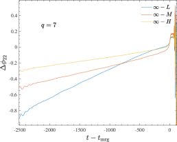
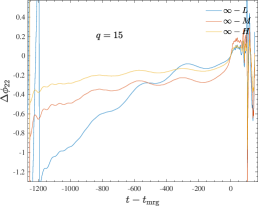
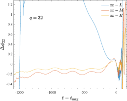
Figure 1: Estimate of the phase uncertainty on our simulations with $q=\{7,15,32\}$: accumulated phase differences between finite resolution waveform data and resolution extrapolated waveform (labelled with $\infty$). We consider three resolutions:Low (L), Medium (M), and High (H). The slope of the linear drift decreases as the resolution increases. The NR-RIT waveforms are aligned at merger time.

Beside the direct use of NR simulations, the analysis of GW sources is mostly done using waveform models that are obtained from the synergy between analytical and numerical relativity results. The effective one body (EOB) approach Buonanno and Damour (1999, 2000); Damour et al. (2000); Damour (2001); Damour et al. (2015) is a way to deal with the general-relativistic two-body problem that, by construction, allows the inclusion of perturbative (e.g. obtained using post-Newtonian methods) and full numerical relativity (NR) results within a single theoretical framework. It currently represents a state-of-the-art approach for modeling dynamics and waveforms from binary black holes, conceptually designed to describe the entire inspiral-merger-ringdown phenomenology of quasicircular binaries Nagar and Rettegno (2019); Nagar et al. (2018); Cotesta et al. (2018); Nagar et al. (2019, 2020); Ossokine et al. (2020); Schmidt et al. (2021) or even eccentric inspirals Chiaramello and Nagar (2020); Nagar et al. (2021a); Nagar and Rettegno (2021) and dynamical captures along hyperbolic orbits Damour et al. (2014); Nagar et al. (2021b, a); Gamba et al. (2021a).

The TEOBResumS model is the EOB waveform model that currently shows the highest level of NR-faithfulness Albertini et al. (2021) against all the spin-aligned NR waveforms available (see also Ref. Akcay et al. (2021); Gamba et al. (2021b) for the precessing case). The model has been tested Nagar et al. (2020); Riemenschneider et al. (2021) against NR simulations available up to $q=18$. Although the model generates waveforms that look qualitatively sane and robust also for larger mass ratios, only a direct comparison with NR data can effectively probe its performance in the large-$q$ regime.

The aim of this paper is to provide EOB/NR waveform comparisons to validate the TEOBResumS model (at least) up to $q=128$. To do so, we exploit the NR waveform data discussed above and presented in Ref. Lousto and Healy (2020). This paper is organized as follows: Section II reviews both the NR waveforms we are going to use and the basics of the EOB model TEOBResumS. Section III exploits various sets of NR data to probe the universal behavior of the multipolar hierarchy of waveform amplitudes at merger, showing consistency with test-mass results. The EOB/NR phasing comparisons are discussed in Sec. IV, while Sec. V reports a few considerations about the impact of NR systematics on informing EOB waveform models. Concluding remarks are collected in Sec. VI. We use geometrized units with $c=G=1$.

II NR and EOB waveform data

Let us start by fixing our waveform conventions. The multipolar decomposition of the strain waveform is given by

$$h_{+}-ih_{\times}={\cal D}_{L}^{-1}\sum_{{\ell m}}h_{{\ell m}}{}_{-2}Y_{{\ell m}}(\theta,\varphi),$$ (1)

where ${\cal D}_{L}$ is the luminosity distance and ${}_{-2}Y_{{\ell m}}(\theta,\varphi)$ are the $s=-2$ spin-weighted spherical harmonics. For consistency with previous works involving the TEOBResumS waveform model, we work with Regge-Wheeler-Zerilli normalized multipoles Nagar and Rezzolla (2005); Nagar et al. (2007) defined as $\Psi_{\ell m}=h_{\ell m}/\sqrt{(\ell+2)(\ell+1)\ell(\ell-1)}$, and each mode is decomposed in amplitude and phase

$$\Psi_{\ell m}=A_{\ell m}\,e^{-i\phi_{\ell m}}\ .$$ (2)

The binary has masses $(m_{1},m_{2})$. We adopt the convention that $m_{1}\geq m_{2}$ and thus we define $q\equiv m_{1}/m_{2}\geq 1$, $M=m_{1}+m_{2}$ and the symmetric mass ratio as $\nu\equiv m_{1}m_{2}/M$.

II.1 NR simulations

We use here the simulations presented in Ref. Lousto and Healy (2020), to which we refer the reader for additional technical details (see also Refs. Healy et al. (2020a); Rosato et al. (2021)). Reference Healy et al. (2020a) explored different gauge choices in the moving puncture formulation in order to improve the accuracy of a linear momentum measure evaluated on the horizon of the remnant black hole produced by the merger of a binary. Similarly, Ref. Rosato et al. (2021) investigated the benefits of adapted gauges to large mass ratio binary black hole evolutions. We found expressions that approximate the late time behavior of the lapse and shift, $(\alpha_{0},\beta_{0})$, and use a position and black hole mass dependent shift damping term, $\eta[\vec{x}_{1}(t),\vec{x}_{2}(t),m_{1},m_{2}]$. We found that this substantially reduces noise generation at the start of the numerical integration and keeps the numerical grid stable around both black holes, allowing for more accuracy with lower resolutions. We tested this gauge in detail in a case study of a binary with a 7:1 mass ratio, and then use 15:1 and 32:1 binaries for a convergence study. NR waveforms Abbott et al. (2016a); Lange et al. (2017) are being directly applied to GW parameter estimation, demonstrating how source parameters for generic BHBs can be inferred based directly on solutions of Einstein’s equations. Specific cases have been performed for the GW150914 and GW170104 Lovelace et al. (2016); Healy et al. (2018); Kumar et al. (2019) events, finding excellent agreement between RIT and SXS Buchman et al. (2012); Chu et al. (2009); Hemberger et al. (2013); Scheel et al. (2015); Blackman et al. (2015); Lovelace et al. (2012, 2011); Mroue et al. (2013); Lovelace et al. (2015); Kumar et al. (2015); Lovelace et al. (2016); Abbott et al. (2016b); Boyle et al. (2019) waveforms up to $\ell=m=5$ modes, but for comparable masses between $q=1/0.85$ and $q=1/0.43$. The direct use of theoretical waveform information to interpret gravitational waves observations and to determine the precise nature of the astrophysical sources has proven to be a remarkable success when applied to O1/O2 BBH events Healy et al. (2020b) and beyond Gayathri et al. (2020). And the recent release of the RIT binary black hole waveform public catalog includes 1881 simulations Healy and Lousto (2022).

We only report here the information that is pertinent for our targeted EOB/NR comparisons. In particular, let us remember that we follow Ref. Healy et al. (2017) to setup quasi-circular initial data that allow our simulations to have a negligible amount of spurious initial junk radiation. Similarly, we use the procedure of Ref. Nakano et al. (2015) to accurately extrapolate the waveform to infinity. The code natively outputs the Weyl scalar $\Psi_{4}$ that is then transformed to the strain by applying a standard integration procedure in the frequency domain Reisswig and Pollney (2011). We consider mass ratios $q=(7,15,32,64,128)$. For $q=(7,15,32)$ we could complete runs at three resolutions, named Low (L), Medium (M) and High (H), so to have a complete convergent series. This allowed us to Richardson-extrapolate the waveform to infinite resolution and thus give an estimate of the phase uncertainty. Figure 1 reports the phase differences between the resolution-extrapolated $\ell=m=2$ waveform (indicated as $\infty$) and each finite resolution. All waveforms are aligned at merger point (marked with $t-t_{\rm mrg}=0$), where merger is defined as the peak of the quadrupolar amplitude $A_{22}$. We remark that the $\Delta\phi_{22}(t)\equiv\phi^{\infty}_{22}-\phi_{22}^{L,M,H}$ is fundamentally a linear function of time during the inspiral up to merger, and its slope decreases as the resolution is increased. This, well known, effect related to resolution will be useful later when interpreting EOB/NR phase comparison. Finally, Fig. 1 indicates that a phase uncertainty $\Delta\phi_{22}$ between $\sim 0.2$ and $\sim 0.4$ rad looks like a reasonable (conservative) error bar estimate on resolution extrapolated waveforms.

II.2 Effective-one-body framework

We use here the most advanced quasi-circular version of the TEOBResumS model Nagar et al. (2020); Riemenschneider et al. (2021), that also includes several subdominant modes completed through merger and ringdown. More precisely, we use here the Matlab private implementation of the model (and not the public one written in $C$ Riemenschneider et al. (2021)) that relies on the iterative determination of the next-to-quasi-circular correction parameters and not on the fits described in Ref. Riemenschneider et al. (2021). Let us recall that this waveform model exploits NR waveform data in two ways. On the one hand, NR waveforms are used to inform two dynamical parameters that enter directly the EOB Hamiltonian (both in the orbital and spin-orbital sector). On the other hand, NR waveform data are used in the description of merger and ringdown via a certain fitting procedure Damour and Nagar (2014) of NR data. The model exploited SXS data up to $q=10$, with five more datasets with $q=18$ Nagar et al. (2020). Test-mass data obtained using Teukode Harms et al. (2014) are also used to inform the fits of amplitude and frequency at peak of each multipole. The resulting TEOBResumS waveform model has been validated against several hundreds of NR simulations, of different accuracy, including mass ratios up to $q=18$. For larger mass ratios the model generates waveforms that looks sane, in general non pathological (excluding extremely spinning cases), but a systematic validation of their quality has not been done so far for the lack of suitable NR data, and it will be the focus of Sec. IV below.

III Multipolar hierarchy at merger

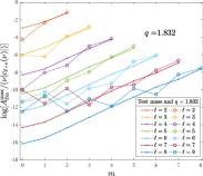
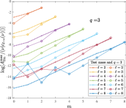
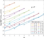
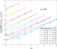
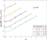
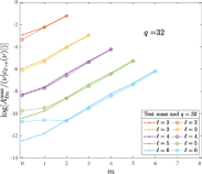
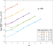
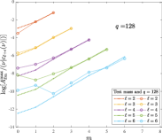
Figure 2: Multipolar hierarchy of merger amplitudes: $\nu$-reduced maximum amplitude for each multipole, Eq. (4) versus $\ell$ and $m$. The test-mass values (dotted lines) are compared with the NR values for various $q$. Up to $q=10$ we use SXS data. For $q>10$ (bottom panels) we use only RIT waveforms. Note the consistency between all the $\ell=m$ modes. The plot highlights the well-known decrease of importance of the subdominant multipoles with $m<\ell$ as the mass ratio is decreased. For each value of $\ell$, an approximate exponential dependence on $m$ is found, with qualitative consistency between the test-mass and the comparable-mass cases. The oscillations present in the SXS $\ell=7$ and $\ell=8$ modes for small values of $m$ denote inaccuracies in the simulations.

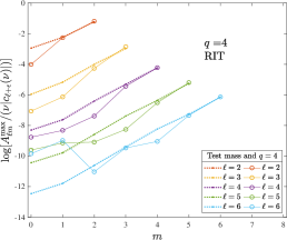
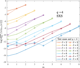
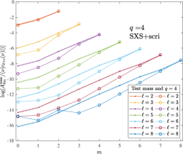
Figure 3: Multipolar hierarchy of merger amplitudes for $q=4$ from RIT data (left panel), standard SXS data (central panel, SXS:BBH:2030 dataset), and SXS waveforms extrapolated to $\mathscr{I}^{+}$ using the python package scri of Ref. Iozzo et al. (2021) (right panel) with the addition of the contribution of the displacement memory as described in Ref. Mitman et al. (2021). Note the improved consistency of the scri-extrapolated data and test-mass data for all $\ell=2$ multipoles as well as for the $\ell=m$ ones.

The multipolar structure of the waveform amplitude at merger has a universal structure that can be described by the mass ratio $\nu$ and an effective spin parameter. This hierarchy emerges when leading order PN expressions are suitably factorized. In particular, Ref. Nagar et al. (2018), pointed out a quasi-universal behavior in the symmetric mass ratio $\nu$ and spin parameter $\hat{S}$ of the $\ell=m=2$ merger frequency (see Fig. 33 therein). Working in the test-mass limit, Ref. Bernuzzi et al. (2011) identified a simple structure of the multipolar peak amplitudes $A_{\ell m}^{\rm max}=\max_{t}(A_{\ell m})$ in terms of the multipolar order $(\ell,m)$,

$$A_{\ell m}^{\rm max}/\nu\approx e^{c_{1}(\ell)m+c_{2}(\ell)\ell},$$ (3)

where the coefficients $c_{i}(\ell)$ are listed in Table VI of Bernuzzi et al. (2011); for $\ell>2$, the coefficient $c_{1}$ is practically independent of $\ell$. Here we show that this structure is present in any BBH multipolar waveform and can be recovered by analytically removing the leading $\nu$ dependence in each multipole. On a practical level, this finding is important to construct the ringdown part of the EOB waveform Damour and Nagar (2014) in order to design accurate and physically motivated fits to NR data.

From PN theory (see e.g. Damour et al. (2009)), the leading $\nu$ dependence of $A_{\ell m}^{\rm max}$ is

$$\hat{\vphantom{\rule{1.0pt}{5.71527pt}}\smash{\hat{A}}}_{\ell m}\equiv\dfrac{A_{\ell m}^{\rm max}}{\nu|c_{\ell+\epsilon}(\nu)|}\,,$$ (4)

where

$$c_{\ell+\epsilon}(\nu)=X_{2}^{\ell+\epsilon-1}+(-)^{m}X_{1}^{\ell+\epsilon-1}\,.$$ (5)

In the expressions above, $\epsilon\equiv\pi(\ell+m)$ is the parity of $\ell+m$, $\epsilon=0$ if $\ell+m$ is even and $\epsilon=1$ if $\ell+m$ is odd. Although this structure is used in Refs. Nagar et al. (2018, 2021a) to accurately fit the multipolar amplitude values around merger, it has not been spelled out explicitly before, and in particular not in connection with test-mass results. Figure 2 contrasts the values of $\hat{\vphantom{\rule{1.0pt}{5.71527pt}}\smash{\hat{A}}}_{\ell m}$ for several comparable mass binaries (solid lines) with the corresponding test-mass values taken from Ref. Bernuzzi et al. (2011) (dotted lines) up to $\ell_{\rm max}=8$, when available. We use the following SXS datasets: SXS:BBH:1354 ($q=1.832$); SXS:BBH:1178 ($q=3$); SXS:BBH:0298 ($q=7$) and SXS:BBH:1107 ($q=10$). Each dataset is taken at the highest resolution available and choosing $N=2$ extrapolation order  Boyle and Mroue (2009), in order to assure a more robust representation of merger and ringdown part. For SXS data we have all multipoles up to $\ell_{\rm max}=8$, while our RIT waveforms are limited to $\ell_{\rm max}=6$ and we only focus on the $m=\ell$ and $m=\ell-1$ modes. From Fig. 2 one sees that the test-mass hierarchy between the modes is preserved also in the comparable-mass case. The figure also highlights the quantitative consistency between the test-mass and comparable-mass $m=\ell$ and $m=\ell-1$ values of $\hat{\vphantom{\rule{1.0pt}{5.71527pt}}\smash{\hat{A}}}_{\ell m}$. We observe a degradation of the accuracy of NR simulations with both low values of $m$ and levels of radiation (high $\ell$).

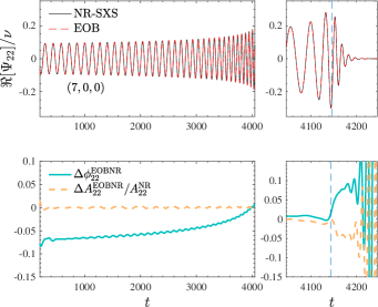
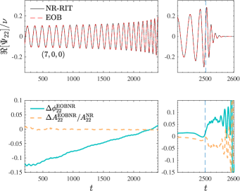
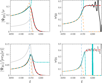
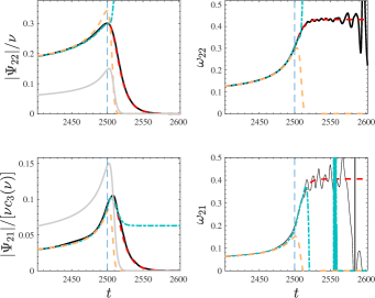
Figure 4: EOB/NR comparison for $q=7$ configuration using either SXS:BBH:0298 (left column) or the resolution-extrapolated RIT data presented here (right column). Waveform are aligned on the frequency interval $[\omega_{L},\omega_{R}]=[0.2,0.3]$, close to merger. The top row report the real part of the $\ell=m=2$ mode as well as the phase difference, $\Delta\phi_{22}^{\rm EOBNR}\equiv\phi^{\rm EOB}_{22}-\phi^{\rm NR}_{22}$ and the relative amplitude difference. The bottom panels compare amplitude and frequencies of both the $(2,2)$ and $(2,1)$ waveform mode. The consistency between the two NR waveforms is remarkable, although the phase accumulated by the RIT one is globally slightly larger, but coherent with the NR uncertainty estimate of Fig. 1.

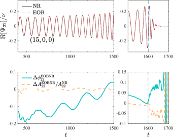
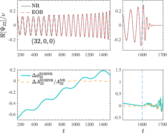
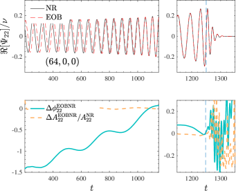
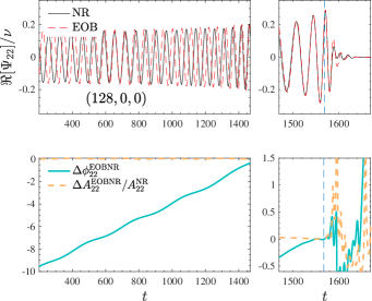
Figure 5: EOB/NR-RIT comparison for various mass ratios. For $q=\{15,32\}$ we use resolution-extrapolated waveforms, while for $q=\{64,128\}$ we adopt the highest resolution available. The waves are aligned in the late inspiral, on the frequency interval $[\omega_{L},\omega_{R}]=[0.2,0.3]$. For each mass ratio, the upper panel compares the real part of the waveforms, while the bottom panel shows the phase difference $\Delta\phi^{\rm EOBNR}_{22}\equiv\phi^{\rm EOB}_{22}-\phi^{\rm NR}_{22}$ and the relative amplitude difference. Note the high EOB/NR consistency during the merger and ringdown phase. For $q=128$ the differences in the ringdown are due to NR inaccuracies.

In Figure 5 we display the EOB vs. NR-RIT waveform comparisons for a sequence of increasing mass ratios, $q=\{15,32,64,128\}$. These naturally show a progressive dephasing and error with increasing $q$.

III.1 Data at $\mathscr{I}^{+}$ and memory effect

Additional insight may be given by considering a different type of numerical waveforms provided in a separate section of the SXS catalog, the Ext-CCE catalog. This section contains asymptotic waveforms whose evolution has been run with with SpEC SpE , and that have been computed in two ways: (i) using the Cauchy-characteristic evolution (CCE) scheme implemented in SpECTRE Moxon et al. (2020) and (ii) using the extrapolation procedure implemented in the python package scri Boyle (2013); Boyle et al. (2014); Boyle (2016). The latter waveforms are crucially augmented by the nonoscillatory memory contribution as described in Mitman et al. Mitman et al. (2021), using a technique that exploits Bondi-Metzner-Sachs (BMS) balance laws. This calculation relies on the extraction from the numerical spacetime of the full set of Weyl scalars, as discussed in Ref. Iozzo et al. (2021). By contrast, CCE proceeds by exploiting Cauchy data yielded by NR simulations as a boundary on a timelike worldtube at finite radius, combining it with an exterior evolution on null hypersurfaces reaching $\mathscr{I}^{+}$. Though these templates should in principle be more accurate, due to difficulties in choosing initial data the waveforms of the kind (i) exhibit spurious oscillations, and are hence unsuited for our purposes. The latest implementation of the SpECTRE CCE module Moxon et al. (2021) is able to extract waveforms either from finished simulations or from a Generalized Harmonic simulation simultaneously running in SpECTRE, but this kind of data is currently not readily available.

Interestingly, Ref. Mitman et al. (2021) proved the consistency between CCE waveforms and extrapolated waveforms improved by the addition of the nonoscillatory memory contribution. The same work also pointed out that the memory calculation turns out to be incorrect by $50\%$ for some unknown reason, starting from the $\ell=3$, $m=0$ contribution (see especially Sec. IIIB.2 therein). Despite these drawbacks and open issues, it is meaningful to perform the same analysis of the $\hat{\vphantom{\rule{1.0pt}{5.71527pt}}\smash{\hat{A}}}_{\ell m}$ quantities using scri-extrapolated waveforms (with the nonoscillatory memory) taken from the Ext-CCE catalog. In this case, the recommended extrapolation order for the strain $h$ data is $N=5$. We focus on $q=4$ nonspinning data: Figure 3, shows the triple comparison between: (i) standard extrapolated $q=4$ SXS data; (ii) the scri-extrapolated data plus the addition of memory and (iii) RIT data. On the one hand, the figure highlights the consistency between SXS and RIT data. On the other hand, the most interesting outcome of the analysis is the much improved consistency between the test-mass and $q=4$ scaled amplitudes $\hat{\vphantom{\rule{1.0pt}{5.71527pt}}\smash{\hat{A}}}_{{\ell m}}$ for $\ell=2$, most remarkably for the $\ell=2$, $m=0$ mode.

IV EOB/NR time-domain phasing comparison

In this section we study the EOB/NR waveform consistency, comparing higher multipoles and mass ratios to reach to an improvement of some EOB fitting parameters of particular relevance for large mass ratios.

IV.1 SXS/RIT/EOB consistency for $q=7$

We start our analysis considering a BBH configuration with $q=7$, a mass-ratio regime where both SXS and RIT data are well under control. A similar consideration applies to the EOB waveform. It is thus instructive to drive a triple comparison SXS/EOB and RIT/EOB so to better learn the differences between the two NR simulations, using the EOB waveform as a reference waveform. For SXS, we use the SXS:BBH:0298 configuration, taken at the highest available resolution and with $N=3$ extrapolation order, since we want to have good control also of the inspiral. For what concerns RIT, we are using resolution extrapolated waveforms so to similarly minimize the phase uncertainty during the inspiral. The comparison is shown in Fig. 4. The waveforms are aligned just before merger time, using our usual alignment procedure Damour and Nagar (2008) that minimizes the EOB/NR phase difference in the frequency interval $[\omega_{L},\omega_{R}]=[0.2,0.3]$. The top row of the figure shows the real part of the $\ell=m=2$ mode, followed (in the second row) by the phase difference and the relative amplitude difference. We recall that the RIT waveform is extrapolated in resolution: the EOB/NR phase difference accumulated in this case is compatible, though larger, than the SXS one, but consistent with the NR uncertainty estimated in the previous section. The picture also highlights the consistency between ringdowns, although the RIT one globally looks more accurate, with a slightly smaller phase difference. This might be traced back to the fact that $(N=2)$-extrapolated SXS data (more accurate during merger and ringdown) were used to construct the ringdown model and not the $N=3$ ones that we are using here. Still, the right panel of Fig. 4 proves the reliability and robustness of the NR-fitting procedure behind the construction of the EOB ringdown model.

The third and fourth rows of Fig. 4 complement the above information showing amplitude and frequencies for both the $\ell=m=2$ and $\ell=2$, $m=1$ modes. Each panel of the figure incorporates several curves: (i) the NR one (black online); (ii) the TEOBResumS one (red online); (iii) the EOB orbital frequency (grey online); (iv) the purely analytical EOB waveform, without NR-tuned next-to-quasi-circular (NQC) corrections nor NR-informed ringdown (orange online); (v) the curve improved by NQC corrections (light-blue online). The figure confirms that RIT data are generally closer to the EOB waveform for both modes as well as it highlights the excellent EOB/NR consistency already achievable with the purely analytical waveform. An important takeaway message of Fig. 4 is that the presence of a linear-in-time EOB/NR phase difference for RIT data during the inspiral does not harm the quality of the merger and ringdown description. This observation will turn out to be useful in the next section, where we will similarly be analyzing RIT data with larger mass ratios.

This general good agreement of SXS and RIT NR waveforms supplements those observed for the sources of GW150914 Lovelace et al. (2016) and GW170104 Healy et al. (2018) for the more comparable mass ratios and up to $\ell=4$ modes.

IV.2 RIT/EOB comparison for large mass ratios

Let us focus now on the $\ell=m=2$ EOB/NR phasing comparisons for $q=\{15,32,64,128\}$. Likewise the $q=7$ case, waveforms are aligned just before merger. For $q=\{15,32\}$ we provide comparisons with the resolution-extrapolated waveform, while for $q=\{64,128\}$ we use the highest resolution available. The plot show a remarkable EOB/NR agreement during merger and ringdown, despite not having used any of this data to inform TEOBResumS. The secular EOB/NR dephasing accumulated during the inspiral is related to the finite resolution of the simulation and it is of no concern at the moment. Note in particular that for $q=15$, the phase difference accumulated towards early frequency is $\Delta\phi^{\rm EOBNR}_{22}\sim-0.2$ rad, that is of the order of the estimated NR uncertainty. The accumulated $\Delta\phi^{\rm EOBNR}_{22}$ is at most of the order of $\sim 1$ rad up to $q=64$. Seen the coherence between $q=\{15,32,64\}$ we think that this value is consistent with a (conservative) error estimate of the NR uncertainty (especially considering that $q=64$ data are not extrapolated in resolution) and thus we can claim that NR data, in a sense, are loosely testing also the radiation-reaction dominated epoch of the waveform up to $q=64$. By contrast, this statement is certainly not correct for $q=128$, that is a much more demanding simulation. Higher resolution will be probably needed here to mutually test the two approaches in this regime. For the moment, we think we can claim that TEOBResumS is here giving the most accurate (approximate) representation we have for an inspiral waveform of a $q=128$ BBH.

IV.3 Higher multipolar waveform modes

Let us finally complete our analysis considering higher modes. The TEOBResumS modes completed through merger and ringdown are $(2,1)$, $(3,3)$, $(3,2)$, $(4,4)$, $(4,3)$ and $(5,5)$. When tested all over the (nonspinning) parameter space, all modes are generated robustly, without evident pathological features, except for the $(5,5)$ one. This mode displays unphysical behavior already for $q\gtrsim 15$. This was already noted by one of us during the first development of the model, in Ref. Nagar et al. (2019) while driving comparisons with a $q=18$ NR dataset obtained using the BAM code from Ref. Husa et al. (2016), although not explicitly reported. Figure 6 is an EOB/NR amplitude and frequency comparison using the $q=18$ BAM data of Ref. Husa et al. (2016). This complements the $\ell=m=2$ mode comparison shown in Fig. 12 of Ref. Nagar et al. (2019). The picture highlights the incorrect behavior of the $\ell=m=5$ mode amplitude after merger. Similarly, the analytical frequency does not match the NR one. Building an improved analytical description of the $\ell=m=5$ mode will be the subject of the next section.

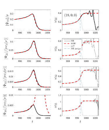
Figure 6: EOB/NR comparison for $q=18$ using the NR data of Ref. Husa et al. (2016). The unphysical behavior of the $\ell=m=5$ mode after merger is evident.

Table 1: Time delay $\Delta t_{{\ell m}}$ between the $\ell=m=2$ NR waveform peak and the corresponding peaks for $\ell=m$ multipoles up to $\ell=6$. The second column indicates the identification number of each simulation from the SXS and RIT waveform catalog. Exception to this are the $q=18$ dataset, obtained in Ref. Husa et al. (2016) using the BAM code, and the test-mass limit waveform obtained using Teukode Harms et al. (2014, 2013).

$\#$	ID	$q$	$\nu$	$\Delta t_{44}$	$\Delta t_{55}$	$\Delta t_{66}$
1	SXS:BBH:1153	1	0.25	3.6587	$\dots$	6.65044
2	SXS:BBH:0198	1.203	0.2479	3.4943	$\dots$	$\dots$
3	SXS:BBH:1354	1.832	0.2284	$\dots$	4.8445	$\dots$
4	SXS:BBH:1166	2	$0.\bar{2}$	$\dots$	4.4172	$\dots$
5	SXS:BBH:0191	2.507	0.2038	2.1388	…	$\dots$
6	SXS:BBH:1178	3	0.139	1.601	4.196	$\dots$
7	SXS:BBH:0197	5.522	0.0988	3.6521	4.6133	4.520
8	SXS:BBH:0298	7	0.1094	3.7126	4.6045	5.2422
9	RIT:BBH:0416	7	0.1094	4.2687	4.6794	4.6301
10	SXS:BBH:0301	9	0.09	4.2998	5.2108	5.7425
11	SXS:BBH:1107	10	0.0826	4.3957	5.3862	6.087
12	RIT:BBH:0373	15	0.0586	4.34	4.7081	4.658
13	BAM Husa et al. (2016)	18	0.0499	4.4054	5.1464	5.8734
14	RIT:BBH:0792	32	0.0294	2.8970	2.9929	2.0056
15	RIT:BBH:0812	64	0.0151	2.946	2.7026	1.996
16	RIT:BBH:0935	128	0.0077	3.524	5.0108	4.4429
17	Teukode	$\infty$	0	5.2828	6.5618	7.7

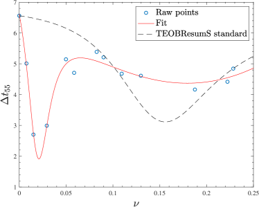
Figure 7: NR points and interpolating fits for the quantities entering the postpeak description of the $(5,5)$ mode. Note the special behavior of the $\Delta t_{55}$ that is necessary to correctly capture the values for $q=32$ and $q=64$. The previously implemented fit (incorrectly informed by other SXS datasets) is superposed for completeness.

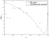
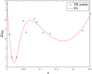
Figure 8: Behavior of the $\Delta t_{44}$ and $\Delta t_{66}$ points of Table 1. For the $\Delta t_{44}$ we also superpose the current fit implemented in TEOBResumS. The differences with the NR data for small values of $\nu$ do not seem to impact the EOB/NR waveform agreement (see Fig. 9). The behavior of $\Delta t_{66}$ is qualitatively analogous to the $\Delta t_{55}$ one.

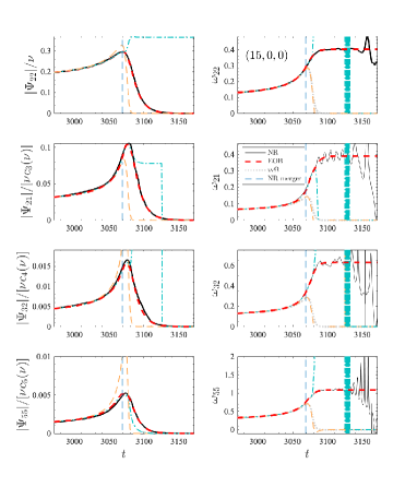
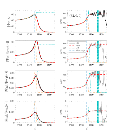
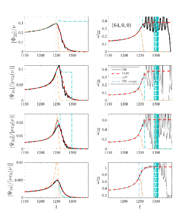
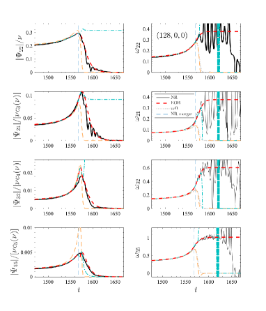
Figure 9: EOB/NR comparison of amplitude and frequency including higher modes. The $\ell=m=5$ mode uses the new ringdown fit described in Sec. IV.3.1. We report the analytical waveform (orange online), the NQC-completed waveform (light-blue online) and the one completed through merger and ringdown (red online).

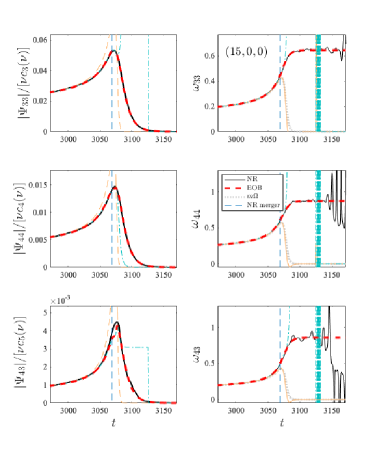
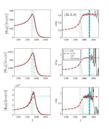
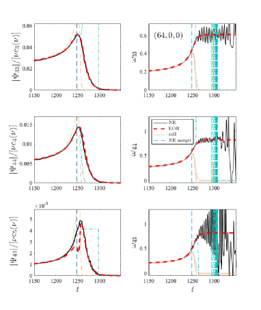
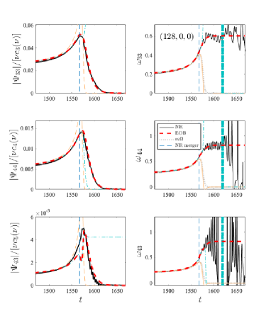
Figure 10: EOB/NR comparison of amplitude and frequency including the higher modes not considered in Fig. 9. Note that the $(4,3)$ amplitude becomes increasingly inaccurate before merger (due to the imperfect action of the next-to-quasi-circular factor) as $q$ increases.We report the analytical waveform (orange online), the NQC-completed waveform (light-blue online) and the one completed through merger and ringdown (red online).

IV.3.1 Improved analytical description of the $\ell=m=5$ merger and ringdown waveform

The ringdown (or better saying, the postpeak) description of each multipole within TEOBResumS is based on the NR-informed fitting procedure introduced in Ref. Damour and Nagar (2014). This approach, originally discussed for the $\ell=m=2$ mode, was extended to higher modes and gives one of the essential building blocks of TEOBResumS Nagar et al. (2019, 2020). The method also yields a stand-alone time-domain waveform model that can be used in targeted ringdown analyses Del Pozzo and Nagar (2017); Carullo et al. (2019), and improvement in the modeling of the amplitude already exists Albanesi et al. (2021). Here we build upon Ref. Nagar et al. (2019) and improve the (nonspinning) fits for the $\ell=m=5$ postpeak waveform presented there. To do so, we (i) use a new sample of carefully chosen SXS datasets, with $N=2$ extrapolation order and mass ratio $1<q\leq 10$; (ii) complement this data with a $q=18$ BAM waveform already used in previous work Nagar et al. (2019) and all the $q=\{15,32,64,128\}$ datasets discussed above. This is essential to correctly connect the comparable-mass regime with the extreme-mass-ratio limit. We present here new fits for the amplitude peak $\hat{A}_{55}$, for the three parameters $(c^{3}_{A},c^{3}_{\phi},c^{4}_{\phi})$ entering the postpeak description (see Ref. Damour and Nagar (2014) for details), and for $\Delta t_{55}$, the time lag between the peaks of the $(2,2)$ and $(5,5)$ modes. This quantity is especially important because it is the one that assures that the postpeak waveform is attached to the inspiral waveform at the correct point.

Following Ref. Nagar et al. (2019), both $\hat{A}_{55}$ and $\Delta t_{55}$ are fitted after factorization of their values in the test-mass limit and, for the amplitude, of the leading-order dependence on $\nu$. We use different SXS simulations depending on the quantity we have to fit. In the left panel of Fig. 7 we show the raw points for $\hat{A}_{55}$ and $(c^{3}_{A},c^{3}_{\phi},c^{4}_{\phi})$, extracted from $q=\{1,1.5,2,3,4,5,6,8,9.89\}$ SXS simulations, with the best-fit functions superposed. They are given by

$$\hat{A}_{55}^{\rm peak} =1-0.97509\nu+11.20088\nu^{2},$$ (6)

$$c^{3}_{A} =-0.59703+9.11875\nu,$$ (7)

$$c^{3}_{\phi} =4.22624-59.69283\nu+373.31260\nu^{2}\ ,$$ (8)

$$c^{4}_{\phi} =1.36397+14.911137\nu.$$ (9)

The accurate representation of $\Delta t_{55}(\nu)$ is a crucial element to assure that the postpeak waveform is attached at the correct place. As a consequence, we were especially careful in selecting the NR datasets that are listed in Table 1. We selected the SXS simulations under the conditions that the values are stable with $\nu$, i.e. small variations of $\nu$ yield small variations in $\Delta t_{55}$. This is not always the case when using data in the SXS catalog and extra care should be exerted in the dataset choice, since the $(5,5)$ mode seems particularly sensitive to the appearance of unphysical effects. The points of Table 1 are shown in the right panel of Fig. 7. We see that the behavior of $\Delta t_{55}$ for $q=(32,64,128)$ is rather complicated and it is necessary to have this data in order to correctly enforce the $\nu\to 0$ limit. The fit for $\Delta t_{55}$ reported in the figure explicitly reads

$$\Delta t_{55}=n_{0}\dfrac{1+n_{1}\nu+n_{2}\nu^{3}+n_{3}\nu^{3}+n_{4}\nu^{4}}{1+d_{1}\nu+d_{2}\nu^{2}}\ ,$$ (10)

where

$$n_{0} =6.6195,$$ (11)

$$n_{1} =-91.2039,$$ (12)

$$n_{2} =2556.5123,$$ (13)

$$n_{3} =-11325.217,$$ (14)

$$n_{4} =27767.2164,$$ (15)

$$d_{1} =-66.0362,$$ (16)

$$d_{2} =1762.4169.$$ (17)

Let us finally briefly comment on the $\Delta t_{44}$ and $\Delta t_{66}$ points listed in Table 1. The $\Delta t_{44}$ points are shown in the left panel of Fig. 8 together with the fit of Ref. Nagar et al. (2020), that is currently implemented in TEOBResumS (dashed line on the plot). We see that, similarly to the $\Delta t_{55}$ case, $\Delta t_{44}$ shows a special behavior for small $\nu$ that is not captured by the fit. Since we have found that this does not have a relevant influence on the modelization of the $\ell=m=4$ mode for large mass ratios (see the corresponding plots in Fig. 9 below), we have decided to keep the standard TEOBResumS fit. The $\Delta t_{66}$ points display the same qualitative behavior of the $\Delta t_{55}$ ones, and thus it is necessary to use a sufficiently flexible rational function to fit them robustly (solid line in the plot). In conclusion, our analysis shows that NR simulations of large mass ratio binaries encode important information that needs to be taken into account so that the TEOBResumS model correctly tends to the test-mass limit. Simpler interpolations to the test-mass limit can eventually introduce systematic effects that may invalidate robust performance all over the parameter space.

IV.3.2 Global comparison

Figure 9 and 10 illustrate the EOB/NR agreement around merger for all modes that are robustly completed through merger and ringdown, i.e.: $(2,2)$, $(2,1)$, $(3,3)$, $(3,2)$, $(4,4)$, $(4,3)$ and $(5,5)$. Note that here, to ease the comparison, we are not using resolution-extrapolated waveform data, but highest resolution data instead. The reason for this choice is that the extrapolation process can fictitiously magnify the oscillations in the frequency that are present during the ringdown in some modes, e.g. the (2,1) mode. Analogously to the $q=7$ case mentioned above, for each mass-ratio and mode reported in Fig. 9 we compare four curves: (i) the NR one (black online); (ii) the purely analytical one (orange online); (iii) the waveform augmented with NQC corrections (light-blue online) and (iv) the full waveform completed with merger and ringdown (red online). We note now the robustness of the $\ell=m=5$ mode, that is modeled using the new NR-informed ringdown fits described above. Note however that some unphysical features appear in the $(4,3)$ mode amplitude as the mass ratio is increased. In this case, the feature is coming from the NQC correction to the amplitude, while the behavior during ringdown is robust and consistent with the NR waveform for any mass ratio. The improvement of the $(4,3)$ mode for large values of the mass ratio will require a new NQC-determination strategy that will be investigated in future work.

V Informing EOB models using NR simulations: hunting for systematics

EOB analytical waveform models are informed by NR simulations. The idea of incorporating in the model strong-field bits of information extracted from NR was suggested already two decades ago Damour et al. (2002), at the dawn of the EOB development. Nowadays, NR-informing EOB models is a crucial step to make them highly faithful with respect to, error-controlled, NR waveform data Damour and Nagar (2009); Nagar et al. (2016); Bohé et al. (2017); Cotesta et al. (2018); Nagar et al. (2019, 2020, 2021a); Nagar and Rettegno (2021); Riemenschneider et al. (2021); Albertini et al. (2021). In particular, the spin-aligned TEOBResumS model incorporates NR information in: (i) the ringdown part, as discussed above; (ii) the NQC corrections to the waveform; (iii) an effective 5PN function $a_{6}^{c}(\nu)$ entering the orbital interaction potential $A(r;\nu)$, i.e. the $\nu$-dependent deformation of the Schwarzschild potential $1-2/r$; (iv) an effective next-to-next-to-next-to-leading order (i.e. at 4.5PN accuracy) function $c_{3}(\nu)$ entering the spin-orbit coupling term of the Hamiltonian. Here we are only dealing with nonspinning configurations, so our interest is limited to $a_{6}^{c}(\nu)$. Reference Nagar et al. (2019) used several SXS datasets to determine $a_{6}^{c}(\nu)$ as

$$a_{6}^{c}(\nu)=n_{0}\dfrac{1+n_{1}\nu+n_{2}\nu^{2}+n_{3}\nu^{3}}{1+d_{1}\nu}\ ,$$ (18)

where the coefficients $(n_{0},n_{1},n_{2},n_{3},d_{1})$ are given by Eqs.(4.3)-(4.7) of Nagar et al. (2019). The (point-wise) determination of this function relies on EOB/NR time-domain phasing comparisons. For each selected value of $q$, $a_{6}^{c}$ is varied manually until the EOB/NR phase agreement is smaller than (or of the same order as) the NR phase uncertainty at merger. For SXS this (probably conservative) error is estimated by taking the difference between two resolutions at merger time. This is done using data extrapolated at infinity with $N=3$ order. For example, for $q=7$, Ref. Nagar et al. (2019) used the SXS:BBH:0298 dataset and the phase uncertainty at merger estimated in this way gives $\delta\phi^{\rm NR}_{\rm mrg}=-0.0775$ rad (see Table I of Nagar et al. (2019)). Figure 11 shows our current state-of-the-art for $q=7$ and SXS:BBH:0298. With $a_{6}^{c}(\nu)$ given by Eq. (18) one has $\Delta\phi^{\rm EOBNR}_{22}\sim-0.244$ rad at merger point, that is of the same order as, but larger than, the corresponding NR uncertainty $\delta\phi^{\rm NR}_{\rm mrg}$ mentioned above. Figure 11 is obtained with $a_{6}^{c}(7/64)\approx-25.562$ from Eq. (18) and delivers an analytic model that is NR-faithful for any purpose. However, the TEOBResumS model is robust and flexible enough to allow us to be even less conservative and actually reach the NR-error level mentioned above. With $a_{6}^{c}=-33$ we get a dephasing at merger $\sim-0.06$ rad, as illustrated in Fig. 12.

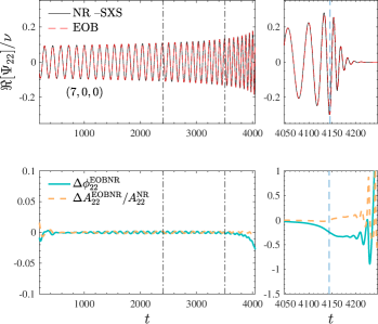
Figure 11: EOB/NR phasing comparison with SXS:BBH:0298 ($q=7$, nonspinning) extrapolated with $N=3$. The vertical dash-dotted lines indicate the alignment region. The phase difference at merger point, $\sim-0.25$ rad, is consistent with (and notably larger than) the NR phase uncertainty $\delta\phi_{\rm mrg}^{\rm NR}=-0.0775$ rad.

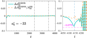
Figure 12: Same EOB/NR phasing comparison with SXS:BBH:0298 of Fig. 11 but using now $a_{6}^{c}=-33$ instead of the value given by Eq. (18): the EOB/NR phase difference at merger is now slightly smaller than the NR phase uncertainty $\delta\phi_{\rm mrg}^{\rm NR}=-0.0775$ rad.

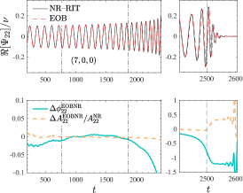
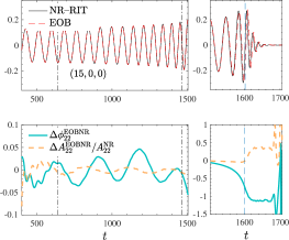
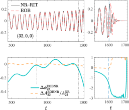
Figure 13: EOB/NR phasing comparison with the waveforms aligned during the early inspiral (vertical dash-dotted lines in the plots). We use here resolution-extrapolated waveforms. For $q=15$ and $q=32$ the comparison is clearly affected by residual initial eccentricity in the simulation.

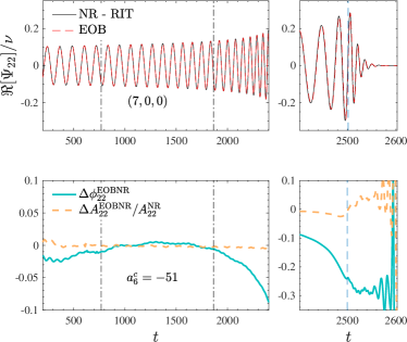
Figure 14: Attempt of NR-informing $a_{6}^{c}$ using the $q=7$ RIT data. For $a_{6}^{c}=-51$ we can reduce the phase difference around merger at $\sim-0.2$ rad, compatible with the NR uncertainty, but this does not affect the phase difference during the inspiral.

Comparing Fig. 11 and 12 one sees that the EOB phasing during the long inspiral is very accurate and the change in $a_{6}^{c}$ only affects the last 5 or 6 orbits. On the basis of this analysis, it seems evident that the level of NR-faithfulness that TEOBResumS can reach depends on the NR uncertainty. Note in this respect that the SXS simulations were not performed with the scope of accurately informing an EOB model. As a consequence, their uncertainties (see e.g. Table I of Ref. Nagar et al. (2019)), obtained by taking the difference of two resolutions, might be either too large or too small for our purposes. In fact, seen all the complications of NR simulations, the best setup to NR-informing the EOB model would be to have at hand different, error-controlled, NR-simulations with equivalent length obtained with different numerical methods. The open question is then to determine to which extent our $a_{6}^{c}(\nu)$ function is independent of the choice of NR data. To attempt an answer, the left panel of Fig. 13 shows the EOB/NR phasing comparison for $q=7$ using RIT NR data extrapolated to infinite resolution. The alignment interval is the same of Fig. 11, but the phase difference accumulated up to merger is $\simeq-1$ rad. Given our error estimate on the $q=7$ RIT waveform in Fig. 1, we expect the NR phase uncertainty to be $\sim 0.3$ rad up to merger. The same conclusion comes from Fig. 4, where both RIT and SXS waveforms show a high degree of consistency among themselves and with the TEOBResumS one when aligned during the late plunge phase. We conclude that the effect in Fig. 13 is related to the numerical errors accumulated during the inspiral, that are probably larger than the SXS ones as already suggested in Fig. 1 above. However, on the basis of the complexity of NR simulations and the very different numerical methods employed to obtain the SXS and RIT data, it is not a priori completely excluded the existence of subtle systematics on both sides. A similar behavior of the phase difference is found also for the $q=32$ and $q=64$ datasets, although it is more compatible with the phase uncertainty.

We conclude this discussion on the dependence of the EOB-tuning on NR data with the following exercise. Let us suppose to fully trust the $q=7$ RIT data and use them as target to inform $a_{6}^{c}$. To do so, we will need a new value of $a_{6}^{c}$, more negative than the current $-25.562$, so to attempt to absorb the phase difference around merger. The result of this exercise is shown in Fig. 14: for $a_{6}^{c}=-51$, the phase difference at merger is reduced to $\sim-0.25$ rad, compatible with the NR phase uncertainty. This tuning however has only a marginal effect on the phase difference during the inspiral, giving thus another indication that one needs improvements on the NR side. This suggests that TEOBResumS is flexible, because it can be tuned to NR when needed, but at the same time rigid and robust, in the sense that it can be used as an auxiliary tool to spot uncertainties (or systematics) in the NR simulations. This is especially true during the inspiral, where TEOBResumS performs best.

From our brief analysis it is clear that TEOBResumS can be robustly informed only using NR simulations with very well controlled (and small, $\lesssim 0.1$ rad) numerical uncertainties. If this seems to be true for SXS, it is not yet the case for our RIT data, although we clearly proved the consistency between the two NR datasets. However, after this first exploration of the large mass ratio regime and comparisons of NR waveforms with those of EOB, we have learned that NR can inform analytic models to improve the fits in this computationally challenging regime. The NR waveforms we used were still first explorations, particularly for $q=(32,64,128)$ and we can now revisit this scenarios with improved accuracy. This is clearly true also for the $q=7$ case, that would serve as an additional benchmark for the corresponding SXS dataset and the related NR-informed quantities within TEOBResumS. We also note that, as indicated by Figs. 11 and 12, shorter NR simulations, with only 10 orbits or less, might be sufficient for additionally informing TEOBResumS, provided that they can be pushed to an accuracy comparable to that of SXS data. Some of the areas of immediate improvements are: (i) the use of improved gauge conditions, as described in Ref. Rosato et al. (2021); (ii) the use of different grid structures than in Lousto and Healy (2020) to emphasize either inspiral or ringdown accuracy; (iii) lengthy simulations with global increase in the resolution, and (iv) reduction of the initial eccentricity with the methods of Buonanno et al. (2011) or Walther et al. (2009).

VI Conclusions

It is generally believed that a state-of-the-art EOB-based waveform model, specifically TEOBResumS, is not robust and trustable outside the so-called domain of calibration, i.e. that region of the parameter space covered by the NR simulations that are used to inform the model. We explicitly proved that this is not true, at least for TEOBResumS. Specifically, we have used recently published NR simulations Lousto and Healy (2020); Healy et al. (2020a); Rosato et al. (2021) of coalescing BBHs with mass ratio from 15 to 128 to validate TEOBResumS in the large mass-ratio regime. This is the first comparison of a semi-analytical waveform model to NR simulations in this corner of the parameter space. The excellent mutual consistency we have found between NR and EOB waveform data gives additional evidence that TEOBResumS is currently the most robust, versatile and NR-consistent EOB-based, spin-aligned, waveform model available. Our work complements then the findings of Refs. Nagar et al. (2020); Riemenschneider et al. (2021); Albertini et al. (2021).

In summary:

• Focusing first on the $(2,2)$ mode, we find an excellent degree of EOB/NR consistency during merger and ringdown up to $q=128$;

• For the inspiral, the numerical truncation error increases progressively with the mass ratio. Still, the EOB/NR dephasings we find are coherent with the expected NR uncertainty;

• Similar consistency through merger and ringdown is found for all available EOB higher modes, $(2,1)$, $(3,3)$, $(3,3)$, $(3,2)$, $(4,4)$ and $(4,3)$, except for the $(5,5)$ mode.

• The native implementation of the $(5,5)$ multipole develops unphysical features at merger and during ringdown, which are related to inaccuracies in the NR-informed fits of Ref. Nagar et al. (2020). These features show up for $q\gtrsim 15$. We thus use the new NR data discussed here to inform an improved $\ell=m=5$ ringdown description. With this new input, the model is tested to be accurate up to $q=128$, and it is smoothly connected with results in the test-particle limit. The new fit discussed here is implemented in the last public version of TEOBResumS.

Our findings highlight the importance of producing highly accurate NR simulations that cover the transition to merger and ringdown in all crucial corners of the parameter space. It also shows the robustness of the analytical scheme that is used to construct the merger-ringdown part of the EOB multipolar waveform Damour and Nagar (2014): once new NR data are available, one can just use them to improve the NR-informed fits, easily removing pathological behaviors that may occur in the analytical waveform around merger. Sparse, but very accurate, NR simulations remain the only tool available to incorporate an accurate merger-ringdown description within waveform models. We hope that the control of quantities like $\Delta t_{{\ell m}}$, the delay between the peak of each multipole and the $\ell=m=2$ one, becomes of primary importance for forthcoming NR simulations.

Let us finally stress that our NR simulations effectively allow us to quantitatively probe only the plunge, merger and ringdown regime of TEOBResumS. In principle we would need long simulations with mass ratio $q>10$, with a typical SXS accuracy, to probe the radiation-reaction driven long inspiral. One should however be aware that the radiation reaction of TEOBResumS incorporates a large amount of PN information, in resummed form, in particular hybridizing $\nu$-dependent terms with test-mass results up to (relative) 6PN accuracy Nagar et al. (2020) for all flux modes up to $\ell=6$. The $\ell=7$ and $\ell=8$ modes, however, rely on less PN information, and an improvement with test-mass data (following Ref. Albanesi et al. (2021)) could be useful. In general, these improvement to the dissipative sector of the model are expected to be important for constructing long-inspiral waveform templates for 3G detectors. By contrast, shorter NR simulations, $\sim 10$ orbits, with reduced eccentricity and accuracy comparable to the SXS ones, would be useful to probe more accurately the full transition from late-inspiral to plunge and merger, possibly informing the EOB dynamics for large mass ratios. This data would also independently benchmark the NR-informed EOB interaction potential, that currently only relies on strong-field information extracted from SXS simulations. This kind of simulations are within reach of our numerical techniques and will be pursued in the future.