Efficient Kernel UCB for Contextual Bandits

Abstract

In this paper, we tackle the computational efficiency of kernelized UCB algorithms in contextual bandits. While standard methods require a $\mathcal{O}(CT^{3})$ complexity where $T$ is the horizon and the constant $C$ is related to optimizing the UCB rule, we propose an efficient contextual algorithm for large-scale problems. Specifically, our method relies on incremental Nyström approximations of the joint kernel embedding of contexts and actions. This allows us to achieve a complexity of $\mathcal{O}(CTm^{2})$ where $m$ is the number of Nyström points. To recover the same regret as the standard kernelized UCB algorithm, $m$ needs to be of order of the effective dimension of the problem, which is at most $\mathcal{O}(\sqrt{T})$ and nearly constant in some cases.

 

Efficient Kernel UCB for Contextual Bandits

 

Houssam Zenati                        Alberto Bietti                        Eustache Diemert

Criteo AI Lab, Inria                        NYU Center for Data Science                        Criteo AI Lab

Julien Mairal                        Matthieu Martin                        Pierre Gaillard

Inria                        Criteo AI Lab                        Inria

1 Introduction

Contextual bandits for sequential decision making have become ubiquitous in many applications such as online recommendation systems (Li et al., 2010). At each round, an agent observes a context vector and chooses an action; then, the environment generates a reward based on the chosen action. The goal of the agent is to maximize the cumulative reward over time, which requires a careful balancing between exploitation (maximizing reward using past observations) and exploration (increasing the diversity of observations).

In this paper, we consider a kernelized contextual bandit framework, where the rewards are modeled by a function in a reproducing kernel Hilbert space (RKHS). In other words, we assume the expected reward to be linear with respect to a joint context-action feature map of possibly infinite dimension. This setup provides flexible modeling choices through the feature map for both discrete and continuous action sets, and exploration algorithms typically rely on constructing confidence sets for the parameter vector and exploring using upper confidence bound (UCB) rules (Li et al., 2010). The extensions to infinite-dimensional feature maps we consider has been introduced by Krause and Ong (2011); Valko et al. (2013) using kernelized variants of UCB, which allow effective exploration even for rich non-parametric reward functions lying in a RKHS, such as smooth functions over contexts and/or actions.

Despite the rich modeling capabilities of such kernelized UCB algorithms, they lack scalability since standard algorithms scale at best as $\mathcal{O}(CT^{3})$ where $T$ is the horizon (total number of rounds) and the constant $C$ is the cost of selecting an action according to the UCB optimization rule. This large cost is due to the need to solve linear systems involving a $t\times t$ kernel matrix at each round $t$, and motivates developing efficient versions of these algorithms for large problems. In supervised learning, a common technique for reducing computation cost is to leverage the fact that the kernel matrix is often approximately low-rank, and to use Nyström approximations (Williams and Seeger, 2001; Rudi et al., 2015). We extend such approximations to the contextual bandit setting, by relying on incremental updates of a dictionary of Nyström anchor points, which allows us to reduce the complexity to $\mathcal{O}(CTm^{2})$, where $m$ is the final number of dictionary elements. In order to preserve a small regret comparable to the vanilla kernel UCB method, $m$ is of the order of an effective dimension quantity, which is typically much smaller than $T$, and at most $\sqrt{T}$.

Closely related to our work, Calandriello et al. (2019, 2020) recently considered Nyström approximations in the non-contextual setting with finite actions, corresponding to a Bayesian optimization problem. Whereas their algorithm is effective when there are no contexts, a direct extension to the contextual setting yields a complexity of $\mathcal{O}(Tm^{3})$, which may be $\mathcal{O}(T^{2.5})$ in the worst case, despite a batching strategy allowing to recompute a new dictionary only about $m$ times. In contrast, our incremental strategy reduces the previous complexity to $\mathcal{O}(Tm^{2})$, and thus at most $\mathcal{O}(T^{2})$.

Even though adopting an incremental strategy for updating the Nyström dictionary may seem to be a simple idea, achieving the previously-mentioned complexity while preserving a regret that is comparable to the original kernel UCB approach is non-trivial. Nyström approximations cause dependencies in the projected kernel matrix that makes it difficult to use martingale arguments, which led Calandriello et al. (2020) to use other mathematical tools that are compatible with updates resampling a new Nyström dictionary. In contrast, we manage to use martingale arguments for an incremental strategy that is less computationally expensive. For that, we extend the standard analysis of the OFUL algorithm for linear bandits (Abbasi-yadkori et al., 2011; Chowdhury and Gopalan, 2017) to the kernel setting with Nyström approximations. In particular, this requires non-trivial extensions of concentration bounds to infinite-dimensional objects. Our analysis also uses the incremental structure of the projections that Calandriello et al. (2019) do not have. This allows us to prove the complexity of our algorithm. Moreover, unlike previous works, we explicit the regret-complexity trade-off under the capacity condition assumption. Finally, we also provide numerical experiments showing that our theoretical gains are also observed in practice.

Algorithm	Regret	Space	Time Complexity
CGP-UCB (Krause and Ong, 2011)	$\mathcal{O}(\sqrt{T}d_{\mathrm{eff}}(\lambda,T))$	$\mathcal{O}(T^{2})$	$\mathcal{O}(CT^{3})$
SupKernelUCB (Valko et al., 2013)	$\mathcal{O}(\sqrt{Td_{\mathrm{eff}}(\lambda,T)\log(C)})$	$\mathcal{O}(T^{2})$	$\mathcal{O}(CT^{3})$
C-BKB (Calandriello et al., 2019)	$\mathcal{O}(\sqrt{T}(\sqrt{\lambda d_{\mathrm{eff}}(\lambda,T)}+d_{\mathrm{eff}}(\lambda,T))$	$\mathcal{O}\left(Td_{\mathrm{eff}}\right)$	$\mathcal{O}\left(T^{2}d_{\mathrm{eff}}^{2}+CTd_{\mathrm{eff}}^{2}\right)$
C-BBKB (Calandriello et al., 2020)	$\mathcal{O}(\sqrt{T}(\sqrt{\lambda d_{\mathrm{eff}}(\lambda,T)}+d_{\mathrm{eff}}(\lambda,T))$	$\mathcal{O}\left(Td_{\mathrm{eff}}\right)$	$\mathcal{O}\left(Td_{\mathrm{eff}}^{3}+CTd_{\mathrm{eff}}^{2}\right)$
K-UCB (ours)	$\mathcal{O}(\sqrt{T}(\sqrt{\lambda d_{\mathrm{eff}}(\lambda,T)}+d_{\mathrm{eff}}(\lambda,T))$	$\mathcal{O}(T^{2})$	$\mathcal{O}(CT^{3})$
EK-UCB (ours)	$\mathcal{O}(\sqrt{T}(\sqrt{\lambda d_{\mathrm{eff}}(\lambda,T)}+d_{\mathrm{eff}}(\lambda,T))$	$\mathcal{O}\left(Td_{\mathrm{eff}}\right)$	$\mathcal{O}(CTd_{\mathrm{eff}}^{2})$

Table 1: Comparison of regret bounds (up to logarithmic factors in $T$) and total time complexity. When the action space is finite, for e.g in SupKernelUCB, we write $C=|\mathcal{A}|$ its cardinality and note that the argmax is obtained in $C$ computations of the UCB rule. Note that the reported regret of CGP-UCB, SupKernel UCB and CBBKB use here the definition of the effective dimension $d_{\mathrm{eff}}(\lambda,T)$ in Eq. (7) which depends on the horizon $T$ and the parameter $\lambda$ (i.e the inverse of the GP noise in CGP-UCB, BKB and BBKB). This effective dimension $d_{\mathrm{eff}}$ is equivalent, up to logarithmic factors, to the information gain used by Srinivas et al. (2010); Calandriello et al. (2020) and the definition used by Valko et al. (2013) (see Appendix D). Moreover, we report the complexities of the contextualized versions of BKB and BBKBs, noting that the non-contextual versions may benefit from certain optimizations when the action space is discrete (Calandriello et al., 2019, 2020).

2 Related Work

UCB algorithms are commonly used in the bandit literature to carefully balance exploration and exploitation by defining confidence sets on unknown reward functions (Lattimore and Szepesvári, 2020). For stochastic linear contextual bandits, the OFUL algorithm (Abbasi-yadkori et al., 2011) obtains improved guarantees compared to previous analyses (e.g., Li et al., 2010) by providing tighter confidence bounds based on self-normalized tail inequalities.

Extensions of linear contextual bandits and UCB algorithms to infinite-dimensional representations of contexts or actions have been studied by Krause and Ong (2011) and Valko et al. (2013) by using kernels and Gaussian processes. While their analyses involve different concepts of effective dimension, it can be shown that these are closely related (see Section 3.3). Valko et al. (2013) notably achieves a better scaling in the horizon in the regret, but requires a finite action space. Chowdhury and Gopalan (2017) improves the analysis of GP-UCB using tools inspired by Abbasi-yadkori et al. (2011) and similar to our analysis of kernel-UCB, though it considers the non-contextual setting. Tirinzoni et al. (2020) in the contextual linear bandit problem use a primal-dual algorithm to achieve an optimal asymptotical regret bound but does not address the issue of computational complexity nor the kernelized setting. Likewise, Camilleri et al. (2021) propose a new estimator in the non-contextual kernelized bandit problem to achieve a tighter regret bound using an elimination algorithm but does no focus on computational efficiency neither.

In the Bayesian experimental design literature Derezinski et al. (2020) propose an efficient sampling scheme using determinant point processes in the non-kernel case and a non-contextual framework. For improving the computational complexity of kernelized UCB procedures in a non-contextual setting as well, Calandriello et al. (2019) use a Nyström approximation of the kernel matrix which is recomputed at each step. Because the corresponding algorithm is not practical when a large number of steps are needed, Calandriello et al. (2020) consider a batched version, which significantly improves its computation and complexity.

In contrast, we use an incremental construction based on the KORS method (Calandriello et al., 2017a), which has been used previously with full information feedback (see also Jézéquel et al., 2019), allowing us to significantly improve the computational complexity of the contextual GP-UCB algorithm, for the same regret guarantee. Such an incremental approach appears to be a key to achieve better complexity than a natural contextual variant of the algorithm of Calandriello et al. (2020), see Table 1, both in theory and in practice (see Section 5). Such an extension is unfortunately non-trivial and requires a different regret analysis, as discussed earlier.

Mutnỳ and Krause (2019) also study kernel approximations for efficient variants of GP-UCB, focusing on random feature expansions. Nevertheless, the number of random features may need to be very large–often exponential in the dimension–in order to achieve good regret, due to a misspecification error which requires stronger, uniform approximation guarantees. Finally, Kuzborskij et al. (2019) also considers leverage score sampling for computational efficiency, but focuses on linear bandits in finite dimension.

3 Warm-up: Kernel-UCB for Contextual Bandits

In this section, we introduce stochastic contextual bandits with reward functions lying in a RKHS, and provide an analysis of the Kernel-UCB algorithm (similar to GP-UCB) which will be a starting point for studying the computationally efficient version in Section 4.

Notations.

We define here basic notations. Given a vector $v\in\mathbb{R}^{d}$ we write its entries $[v_{i}]_{1\leq i\leq d}$ and we will write $v^{\top}w$ or $\langle v,w\rangle$ the dot product for elements in $\mathbb{R}^{d}$ and in the Hilbert space $\mathcal{H}$. We denote by $\|\cdot\|$ the Euclidean norm and the norm in $\mathcal{H}$. The conjugate transpose for a linear operator $L$ on $\mathcal{H}$ is denoted by $L^{*}$. For two operators $L,L^{\prime}$ on $\mathcal{H}$, we write $L\preccurlyeq L^{\prime}$ when $L-L^{\prime}$ is positive semi-definite and we use $\lesssim$ for approximate inequalities up to logarithmic multiplicative or additive terms. A summary of the notations is provided in Appendix A.

3.1 Setup

In the contextual bandit problem, at each time $t$ in $1,\dots,T$, where $T$ is the horizon, for each context $x_{t}$ in $\mathcal{X}$, an action $a_{t}$ in $\mathcal{A}$ is chosen by an agent and induces a reward $r_{t}$ in $\mathbb{R}$. The input and action spaces $\mathcal{X}$ and $\mathcal{A}$ can be arbitrary (e.g., finite or included in $\mathbb{R}^{d}$ for some $d\geq 1$). Note that $\mathcal{A}$ may change over time, but we keep it fixed here for simplicity.

In this paper, we focus on stochastic kernel contextual bandits and assume that there exists a reproducing kernel Hilbert space (RKHS) $\mathcal{H}$ such that

$$r_{t}=\langle\theta^{*},\phi(x_{t},a_{t})\rangle+\varepsilon_{t}\,,$$

where $\varepsilon_{t}$ are i.i.d. centered subGaussian noise, $\theta^{*}\in\mathcal{H}$ is an unknown parameter, and $\phi:\mathcal{X}\times\mathcal{A}\to\mathcal{H}$ is a known feature map associated to $\mathcal{H}$. It satisfies

$$\langle\phi(x,a),\phi(x^{\prime},a^{\prime})\rangle=k\big{(}(x,a),(x^{\prime},a^{\prime})\big{)}\,,$$

where $k$ is a positive definite kernel associated to $\mathcal{H}$. We assume $k$ to be bounded, i.e., there exists $\kappa>0$ such that $k(s,s)\leq\kappa^{2}$ for any $s\in\mathcal{X}\times\mathcal{A}$.

Thus, the goal of the agent is, given the previously observed contexts, actions and rewards $(x_{s},a_{s},r_{s})_{s=1\dots t-1}$ and the current context $x_{t}$, to choose an action $a_{t}$ in order to minimize the following regret after $T$ rounds

$$R_{T}:=\operatorname{\mathbb{E}}\left[\sum_{t=1}^{T}\max_{a\in\mathcal{A}}\langle\theta^{*},\phi(x_{t},a)\rangle-\sum_{t=1}^{T}r_{t}\right].$$ (1)

3.2 Algorithm: Kernel-UCB

Upper confidence algorithm (UCB) algorithms maintain for each possible action an estimate of the mean reward as well as a confidence interval around that mean, and then chooses at each time the highest upper confidence bound. Formally, if we have a confidence set $\mathcal{C}_{t}\subset\mathcal{H}$ based on samples $(x_{t^{\prime}},a_{t^{\prime}},y_{t^{\prime}})$, for $t^{\prime}\in\{1,\ldots,t-1\}$ that contains the unknown parameter vector $\theta^{*}$ with high probability, we may define

$$\text{K-UCB}_{t}(a)=\max_{\theta\in\mathcal{C}_{t}}\langle\theta,\phi(x_{t},a)\rangle$$ (2)

as an upper bound on the mean pay-off $\langle\theta^{*},\phi(x_{t},a)\rangle$ of $a$. To choose the highest upper confidence bound from the confidence set at time $t$, the algorithm then selects:

$$a_{t}\in\operatorname*{arg\,max}_{a\in\mathcal{A}}\text{K-UCB}_{t}(a).$$ (3)

We then build an empirical estimate of the unknown quantity $\theta^{*}$ using regression. More precisely in the kernelized setting, we use the regularized least square estimator with

$$\hat{\theta}_{t}\in\operatorname*{arg\,min}_{\theta\in\mathcal{H}}\Big{\{}\sum_{s=1}^{t}\left(\langle\theta,\phi(x_{s},a_{s})\rangle-r_{s}\right)^{2}+\lambda\|\theta\|^{2}\Big{\}}\,.$$ (4)

Rearranging the terms $\varphi_{s}=\phi(x_{s},a_{s})$ and writing $V_{t}=\sum_{s=1}^{T}\varphi_{s}\otimes\varphi_{s}+\lambda I$, we obtain that the analytical solution for Eq. (4) is $\hat{\theta}_{t}=V_{t}^{-1}\sum_{s=1}^{t}\varphi_{s}r_{s}$. The previous solution from time $t-1$ then defines the center of the ellipsoidal confidence set

$$\mathcal{C}_{t}=\{\theta\in\mathcal{H}:\|\theta-\hat{\theta}_{t-1}\|_{V_{t-1}}\leq\beta_{t}(\delta)\}.$$ (5)

where $\|\theta\|_{V}^{2}=\theta^{\top}V\theta$, and $\beta_{t}(\delta)$ is its radius (see Lemma 8). With $\mathcal{C}_{t}$ in that form, we can write the solution of Eq. (2) as

$$\text{K-UCB}_{t}(a)=\langle\hat{\theta}_{t-1},\phi(x_{t},a)\rangle+\beta_{t}(\delta)^{1/2}\|\phi(x_{t},a)\|_{V_{t-1}^{-1}}.$$ (6)

Indeed, by defining $B_{2}=\{x\in\mathbb{R}^{d}:\|x\|_{2}\leq 1\}$ the unit ball with the Euclidean norm, it is easy to see that $\mathcal{C}_{t}=\hat{\theta}_{t}+\beta_{t}(\delta)^{1/2}V_{t-1}^{-1/2}B_{2}$. Then, for $\theta\in B_{2}$ maximising the quantity $\langle\theta,\phi(x_{t},a)\rangle=\phi(x_{t},a)^{\top}\hat{\theta}_{t-1}+\beta_{t}(\delta)^{1/2}\phi(x_{t},a)^{\top}V_{t-1}^{-1/2}\theta$ gives Eq. (6).

3.3 Regret analysis

We provide an analysis of the regret of the kernelized UCB rule in Eq. (6) using standard statistical analysis definitions of the effective dimension.

Let us write the operator $\Phi_{t}:\mathcal{H}\rightarrow\mathbb{R}^{t}$ such that $\Phi_{t}^{*}=\left[\varphi_{1},\dots\varphi_{t}\right]$, where $\varphi_{i}=\phi(x_{i},a_{i})$ for $i\in[1,t]$. Let us define $K_{t}$ the kernel matrix associated to kernel $k$ and the set of pairs $(x_{1},a_{1}),\dots,(x_{t},a_{t})$, $K_{t}=\Phi_{t}\Phi_{t}^{*}$ is a $t\times t$ matrix. We define the effective dimension of a kernel matrix as in Hastie et al. (2001) and will use the following in our work.

Definition 3.1.

The effective dimension of the matrix $K_{T}$ is defined as,

$$d_{\mathrm{eff}}(\lambda,T)\vcentcolon=\operatorname{Tr}(K_{T}(K_{T}+\lambda I_{T})^{-1})\,.$$ (7)

In what follows, for simplicity of notation, we abbreviate $d_{\mathrm{eff}}(\lambda,T)$ to $d_{\mathrm{eff}}$ unless we use different parameters on $d_{\mathrm{eff}}$. To extend the analysis of OFUL (Abbasi-yadkori et al., 2011) to the contextual kernel UCB algorithm, we will use the following proposition that has been proved and used by Jézéquel et al. (2019).

Proposition 3.1.

For any horizon $T\geq 1,\lambda>0$ and all input sequences $(x_{1},a_{1}),\dots,(x_{T},a_{T})$

$$\sum_{k=1}^{T}\log\left(1+\dfrac{\lambda_{k}(K_{T})}{\lambda}\right)\leq\log\left(e+\dfrac{eT\kappa^{2}}{\lambda}\right)d_{\mathrm{eff}}\,,$$

where $\lambda_{k}(K_{T})$ denotes the $k$-th largest eigenvalue of $K_{T}$.

We now provide a regret bound extending the analysis of Abbasi-yadkori et al. (2011) to the kernel setting. In particular, we start by providing an upper bound on the ellipsoid greater axis.

Lemma 3.1.

Let $\delta\in(0,1)$ and define $\beta_{t+1}(\delta)$ by

$$\sqrt{\lambda}\|\theta^{*}\|+\sqrt{2\log\frac{1}{\delta}+\log\left(e+\dfrac{et\kappa^{2}}{\lambda}\right)d_{\mathrm{eff}}}.$$

Then, with probability at least $1-T\delta$, for all $t\in[T]$

$$\big{\|}\hat{\theta}_{t}-\theta^{*}\big{\|}_{V_{t}}\leq\beta_{t+1}(\delta).$$ (8)

We use this lemma (which relies on Proposition 3.1 whose proof is in Appendix B.1) to bound the distance between the estimated parameter $\hat{\theta}_{t}$ at each round $t$ and the true parameter $\theta^{*}$. By combining this result with Proposition 3.1, we then prove the following theorem that extends the LinUCB upper bound result from Lattimore and Szepesvári (2020).

Theorem 3.1.

Let $T\geq 2$ and $\theta^{*}\in\mathcal{H}$. Assume that $|\langle\phi(x,a),\theta^{*}\rangle|\leq 1$ for all $a\in\bigcup_{t=1}^{T}\mathcal{A}_{t}\subset\mathcal{A}$ and $x\in\mathcal{X}$. Then, the K-UCB rule defined in Eq. (3) for the choice $\mathcal{C}_{t}$ as in (5) with parameter $\lambda>0$, and $\delta=1/T^{2}$, satisfies the pseudo-regret bound

$$R_{T}\lesssim\sqrt{T}\Big{(}\|\theta^{*}\|\sqrt{\lambda d_{\mathrm{eff}}}+d_{\mathrm{eff}}\Big{)}\,,$$

where $\lesssim$ hides logarithmic factors in $T$.

The proof of Theorem 3.1 and the precise statement of the regret bound are given in Appendix B.1.

In particular, assuming the norm of the true parameter $\theta^{\star}$ to be bounded, we obtain the following corollary with a capacity condition on the effective dimension.

Corollary 3.1.

Assuming the capacity condition $d_{\mathrm{eff}}\leq(T/\lambda)^{\alpha}$ for $0\leq\alpha\leq 1$ , the regret of K-UCB is bounded as $R_{T}\lesssim T^{\frac{1+3\alpha}{2+2\alpha}}$ with an optimal $\lambda\approx T^{\frac{\alpha}{1+\alpha}}$.

As an example, if we consider a kernel that is a tensor product between a linear kernel on contexts and a Sobolev-type kernel (e.g., a Matern kernel) of order $s$ on actions, with $s>d/2$ (where $d$ is the dimension of the continuous action space), then we may consider that the kernel eigenvalues decay as $i^{-2s/d}$, leading to an effective dimension as above with $\alpha=d/2s$, and a regret of $T^{\frac{1}{2}\frac{2s+3d}{2s+d}}$.

Discussion.

We note that this regret is not optimal for such problems, but matches the regret of most other kernel or Gaussian process optimization algorithms (see, e.g., Scarlett et al., 2017). More precisely, our analysis recovers classical rates of the GP-UCB algorithm (Srinivas et al., 2010; Chowdhury and Gopalan, 2017), and extends them to the contextual bandit setting. We note that the analysis of Chowdhury and Gopalan (2017) further removes some logarithmic factors, and similar improvements may be obtained in our setting since it is based on similar tools. The SupKernelUCB algorithm by Valko et al. (2013) obtains improved dependencies on $T$ in the regret bounds, but requires a finite set of actions, and therefore is not directly comparable to ours. The CGP-UCB algorithm by Krause and Ong (2011) obtains similar results to ours in the contextual setting, but uses a different analysis. Our result is therefore not new, and our analysis is meant as a starting point for the efficient variant based on incremental Nyström approximations, which will be introduced in the sequel.

We note that these works use different notions than our effective dimension $d_{\mathrm{eff}}$ to characterize complexity, namely the information gain

$$\gamma(\lambda,t)=\dfrac{1}{2}\log\left(\det\left(I+\dfrac{1}{\lambda}K_{t}\right)\right)$$

used by Krause and Ong (2011) as well as the different effective dimension definition in (Valko et al., 2013)

$$\tilde{d}(\lambda,t)~{}=~{}\min\{j:j\lambda\log T\geq\sum_{k>j}\lambda_{k}(K_{t})\}.$$

It can be shown that these are equivalent up to logarithmic factors to our definition of the effective dimension $d_{\mathrm{eff}}$ (see Appendix D). This allows us to compare up to logarithmic factors the algorithm regrets, as shown in Table 1.

4 Efficient Kernel-UCB

In this section, we introduce our efficient kernelized UCB (EK-UCB) algorithm based on incremental Nyström projections. We begin by extending the ellipsoidal confidence bounds from the previous section to the case with projections on finite-dimensional linear subspaces of the RKHS. Then, we present our main algorithm and analyze its complexity and regret.

4.1 Upper confidence bounds with projections

In this section, we study the UCB updates and corresponding high-probability confidence bounds for our EK-UCB algorithm. Because these steps do not depend on a specific choice of projections, we consider generic projection operators onto subspaces of the RKHS, noting that the next sections will consider specific choices based on Nyström approximations.

At round $t\geq 1$, we consider a generic subspace $\tilde{\mathcal{H}}_{t}$ of $\mathcal{H}$, and let $P_{t}:\mathcal{H}\rightarrow\tilde{\mathcal{H}}_{t}$ be the orthogonal projection operator on $\tilde{\mathcal{H}}_{t}$, so that $P_{t}\mathcal{H}=\tilde{\mathcal{H}}_{t}$. For a fixed regularization parameter $\lambda>0$, we consider the following regularized estimator restricted to $\tilde{\mathcal{H}}_{t}$:

$$\tilde{\theta}_{t}\in\operatorname*{arg\,min}_{\theta\in\tilde{\mathcal{H}}_{t}}\bigg{\{}\sum_{s=1}^{t}\left(\langle\theta,\phi(x_{s},a_{s})\rangle-r_{s}\right)^{2}+\lambda\|\theta\|^{2}\bigg{\}}.$$ (9)

Define $\tilde{V}_{t}=\sum_{s=1}^{t}P_{t}\varphi_{s}\otimes P_{t}\varphi_{s}+\lambda I$, which may be written $\tilde{V}_{t}=P_{t}F_{t}P_{t}+\lambda I$ where $F_{t}=\Phi_{t}^{*}\Phi_{t}:\mathcal{H}\to\mathcal{H}$ is the covariance operator. Recalling the notation $Y_{t}=(r_{1},\dots,r_{t})^{\top}$, we obtain that $\tilde{\theta}_{t}=\tilde{V}_{t}^{-1}P_{t}\Phi_{t}^{*}Y_{t}$. We may then define the following ellipsoidal confidence set:

$$\tilde{\mathcal{C}}_{t}\vcentcolon=\big{\{}\theta\in\mathcal{H}:\|\theta-\tilde{\theta}_{t-1}\|_{\tilde{V}_{t-1}}\leq\tilde{\beta}_{t}(\delta)\big{\}}\,,$$ (10)

for some radius $\tilde{\beta}_{t}(\delta)$ to be specified later. Note that the ellipsoid is not necessarily contained inside the projected space $\tilde{\mathcal{H}}_{t}$, and may in fact include $\theta^{*}$ even if $\theta^{*}\notin\tilde{\mathcal{H}}_{t}$. This is a crucial difference with random feature kernel approximations (Mutnỳ and Krause, 2019), for which a standard confidence set would be finite dimensional, and thus generally does not include $\theta^{*}$; this leads to larger regret due to misspecification, unless the number of random features is very large in order to ensure good uniform approximation. We may then define the following upper confidence bounds, which still rely on the original feature map $\phi$:

$$\text{EK-UCB}_{t}(a)\vcentcolon=\max_{\theta\in\tilde{\mathcal{C}}_{t}}\langle\theta,\phi(x_{t},a)\rangle.$$ (11)

This may again be written in closed form as

$$\text{EK-UCB}_{t}(a)=\langle\hat{\theta}_{t-1},\phi(x_{t},a)\rangle+\tilde{\beta}_{t}(\delta)^{1/2}\|\phi(x_{t},a)\|_{\tilde{V}_{t-1}^{-1}}.$$

We note that for appropriate choices of $\tilde{\mathcal{H}}_{t}$, such a quantity can be explicitly computed using the kernel trick, as we discuss in Section 4.3. The following lemma shows that $\tilde{\mathcal{C}}_{t}$ is a valid confidence set, which contains $\theta^{*}$ with high probability, provided that the projection captures well the dominating directions in the covariance operator.

Lemma 4.1.

Let $\delta\in(0,1)$. Define $\tilde{\beta}_{t+1}(\delta)$ as

$$\left(\sqrt{\lambda}+\sqrt{\mu_{t}}\right)\|\theta^{*}\|+\sqrt{4\log\frac{1}{\delta}+2\log\left(e+\dfrac{et\kappa^{2}}{\lambda}\right)d_{\mathrm{eff}}},$$

where $\mu_{t}\vcentcolon=\|(I-P_{t})F_{t}^{1/2}\|^{2}$. Then, with probability at least $1-T\delta$, for all $t\in[T]$

$$\big{\|}\tilde{\theta}_{t}-\theta^{*}\big{\|}_{\tilde{V}_{t}}\leq\tilde{\beta}_{t+1}(\delta).$$ (12)

The quantity $\mu_{t}$ controls how well the projection operator $P_{t}$ captures the dominating eigen-directions of the covariance operator, and should be at most of order $\lambda$ in order for the confidence bounds to be nearly as tight as for the vanilla K-UCB algorithm. The next section further discusses how this quantity is controlled with incremental Nyström projections.

4.2 Learning with incremental Nyström projections

We now consider specific choices of the projections $P_{t}$ and subspaces $\tilde{\mathcal{H}}_{t}$ obtained by Nyström approximation (Williams and Seeger, 2001; Rudi et al., 2015). In particular, the spaces $\tilde{\mathcal{H}}_{t}$ now take the form

$$\tilde{\mathcal{H}}_{t}=\text{Span}\big{\{}\phi(s),s\in\mathcal{Z}_{t}\big{\}},$$ (13)

where $\mathcal{Z}_{t}\subset\{(x_{1},a_{1}),\dots(x_{t},a_{t})\}$ is a dictionary of anchor points taken from the previously observed data. Our approach consists of constructing the dictionaries $\mathcal{Z}_{t}$ incrementally, by adding new observed examples $(x_{t},a_{t})$ on the fly when deemed important, so that we have $\mathcal{Z}_{1}\subset\mathcal{Z}_{2}\dots\subset\mathcal{Z}_{t}$. We achieve this using the Kernel Online Row Sampling (KORS) algorithm of Calandriello et al. (2017a), shown in Algorithm 1, which decides whether to include a new sample $s_{t}=(x_{t},a_{t})$ by flipping a coin with probability proportional to its leverage score (Mahoney and Drineas, 2009). More precisely, an estimate $\tilde{\tau}$ of the leverage score that uses the state feature $\varphi_{t}$ and parameters $\mu,\varepsilon$ is used to assess how a given state is useful to characterize the dataset. More details on the KORS algorithm are given in Appendix E.

Input: Time $t$, past dictionary $\mathcal{Z}$, context-action $s_{t}$, regularization $\mu$, accuracy $\varepsilon$, budget $\gamma$

Compute the leverage score $\tilde{\tau}_{t}$ from $\mathcal{Z},s_{t},\mu,\varepsilon$ ;

Compute $\tilde{p}_{t}=\min\{\gamma\tilde{\tau}_{t},1\}$ ;

Draw $z_{t}\sim\mathcal{B}(\tilde{p}_{t})$ and if $z_{t}=1$, add $s_{t}$ to $\mathcal{Z}$;

Result: Dictionary $\mathcal{Z}$

Algorithm 1 Incremental KORS subroutine

We state the following proposition of Calandriello et al. (2017a, Theorem 1, with $\varepsilon=1/2$), which will be useful for our regret and complexity analyses.

Proposition 4.1.

Let $\delta>0$, $n\geq 1$, $\mu>0$. Then the sequence of dictionaries $\mathcal{Z}_{1}\subset\mathcal{Z}_{2}\subset\dots\mathcal{Z}_{T}$ learned by KORS with parameters $\mu>0,\varepsilon=1/2$ and $\gamma=12\log(T/\delta)$ satisfies with probability $1-\delta$, $\forall t\geq 1$

$$\|(I-P_{t})F_{t}^{1/2}\|^{2}\leq\mu\ \text{ and }\ |\mathcal{Z}_{t}|\leq 9d_{\mathrm{eff}}(\mu,T)\log(2T/\delta)^{2}\,.$$

Additionally, the algorithm runs in $\mathcal{O}(d_{\mathrm{eff}}(\mu,T)^{2})$ time and $\mathcal{O}(d_{\mathrm{eff}}(\mu,T)^{2}\log(T)^{4})$ space per iteration.

This result shows that when choosing $\mu\approx\lambda$, then KORS will maintain dictionaries of size at most $d_{\mathrm{eff}}$ (up to log factors), while guaranteeing that the confidence bounds studied in Section 4.1 are nearly as good as for the case of K-UCB.

4.3 Implementation and complexity analysis

Here, we analyze the complexity of the algorithm and describe its practical implementation. Recall that at each round $t$ the agent chooses an action $a$ that maximises the UCB rule $\mu_{t,a}+\tilde{\beta}_{t}\sigma_{t,a}$ where we use Eq. (11) to reformulate the mean term $\mu_{t,a}=\langle\hat{\theta}_{t-1},\phi(x_{t},a)\rangle$ and the variance term $\sigma_{t,a}^{2}=\|\phi(x_{t},a)\|_{\tilde{V}_{t-1}^{-1}}^{2}$. We use the representer theorem on the projection space $\mathcal{H}_{t}$ to derive efficient computations of the latter two terms instead of using a kernel trick with $t\times t$ gram matrices. Indeed, in the next proposition, we prove that the two terms can be expressed with $m_{t}\times m_{t}$ matrices instead, where $m_{t}=|\mathcal{Z}_{t}|$ is the size of the dictionary at time $t$. We use the notations $K_{\mathcal{S}_{t}}(s^{\prime})$ for the kernel column vector $[k(s_{1},s^{\prime}),\dots,k(s_{t},s^{\prime})]^{\top}$, where $\mathcal{S}_{t}=\{s_{i}\}_{i=1\dots t}$ are the past states, and $K_{\mathcal{A},\mathcal{B}}$ for the matrix of kernel evaluations $[k(s,s^{\prime})]_{s\in\mathcal{A},s^{\prime}\in\mathcal{B}}$.

Proposition 4.2.

At any round $t$, by considering $s_{t,a}=~{}(x_{t},a)$, the mean and variance term of the EK-UCB rule can be expressed with:

$$\Gamma_{t} =K_{\mathcal{Z}_{t-1}\mathcal{S}_{t-1}}Y_{t-1}$$

$$\Lambda_{t} =\left(K_{\mathcal{Z}_{t-1}\mathcal{S}_{t-1}}K_{\mathcal{S}_{t-1}\mathcal{Z}_{t-1}}+\lambda K_{\mathcal{Z}_{t-1}\mathcal{Z}_{t-1}}\right)^{-1}$$

$$\tilde{\mu}_{t,a} =K_{\mathcal{Z}_{t-1}}(s_{t,a})^{\top}\Lambda_{t}\Gamma_{t}$$

$$\Delta_{t,a} =K_{\mathcal{Z}_{t-1}}(s_{t,a})^{\top}\left(\Lambda_{t}-\frac{1}{\lambda}K_{\mathcal{Z}_{t-1}\mathcal{Z}_{t-1}}^{-1}\right)K_{\mathcal{Z}_{t-1}}(s_{t,a})$$

$$\tilde{\sigma}_{t,a}^{2} =\frac{1}{\lambda}k(s_{t,a},s_{t,a})+\Delta_{t,a}.$$

The algorithm then runs in a space complexity of $\mathcal{O}(Tm)$ and a time complexity of $\mathcal{O}(CTm^{2})$.

Input: $T$ the horizon, $\lambda$ regularization and exploration parameters, $k$ the kernel function, $\varepsilon>0,\gamma>0$

Initialization;

Context $x_{0}$, $a_{0}$ chosen randomly and reward $r_{0}$ ;

$\mathcal{S}=\{(x_{0},a_{0})\},Y_{\mathcal{S}}=[r_{0}]$ $\mathcal{Z}=\{(x_{0},a_{0})\}$ ;

$\Lambda_{t}=\left(K_{\mathcal{Z}\mathcal{S}}K_{\mathcal{S}\mathcal{Z}}+\lambda K_{\mathcal{Z}\mathcal{Z}}\right)^{-1}$ $\Gamma_{t}=K_{\mathcal{Z}\mathcal{S}}Y_{\mathcal{S}}$ ;

for $t=1$ to $T$ do

       Observe context $x_{t}$ ;

       Choose $\tilde{\beta}_{t}$ (e.g as in Lem. 12, and $\delta=\frac{1}{T^{2}}$) ;

       Choose $a_{t}\leftarrow\operatorname*{arg\,max}_{a\in\mathcal{A}}\tilde{\mu}_{t,a}+\tilde{\beta}_{t}\tilde{\sigma}_{t,a}$ ;

       $\tilde{\mu}_{t,a}\leftarrow K_{\mathcal{Z}}(s_{t,a})^{\top}\Lambda_{t}\Gamma_{t}$ ;

       $\Delta_{t,a}=K_{\mathcal{Z}}(s_{t,a})^{\top}\left(\Lambda_{t}-\frac{1}{\lambda}K_{\mathcal{Z}\mathcal{Z}}^{-1}\right)K_{\mathcal{Z}}(s_{t,a})$  $\tilde{\sigma}_{t,a}^{2}\leftarrow\frac{1}{\lambda}k(s_{t,a},s_{t,a})+\Delta_{t,a}$ ;

      

      Observe reward $r_{t}$ and $s_{t}\leftarrow(x_{t},a_{t})$ ;

       $Y_{\mathcal{S}}\leftarrow[Y_{\mathcal{S}},r_{t}]^{\top},\mathcal{S}\leftarrow\mathcal{S}\cup\{s_{t}\}$ ;

       $\mathcal{Z}^{\prime}\leftarrow\text{KORS}(t,\mathcal{Z},K_{\mathcal{Z}}(s_{t}),\lambda,\varepsilon,\gamma)$ ;

       if $\mathcal{Z}^{\prime}=\mathcal{Z}$  then

             Incremental inverse update $\Lambda_{t}$ with $s_{t}$;

             $\Gamma_{t+1}\leftarrow\Gamma_{t}+r_{t}K_{\mathcal{Z}}(s_{t})$ ;

            

       end if

      else

             $z=\mathcal{Z}^{\prime}\ \backslash\ \mathcal{Z}$ ;

             Incremental inverse update $\Lambda_{t}$ with $s_{t},z$ ;

             Incremental inverse update $K_{\mathcal{Z}\mathcal{Z}}^{-1}$ with $z$;

             $\Gamma_{t+1}\leftarrow[\Gamma_{t}+r_{t}K_{\mathcal{Z}}(s_{t}),\ K_{\mathcal{S}}(z)^{\top}Y_{\mathcal{S}}]^{\top}$

       end if

      

end for

Algorithm 2 Efficient Kernel UCB

In our algorithm, the incremental updates of the projections allow us to derive rank-one updates of the expressions $\Lambda_{t},\Gamma_{t},K_{\mathcal{Z}_{t}\mathcal{Z}_{t}}^{-1}$ in all cases. First, when the dictionary does not change (i.e $P_{t}=P_{t-1}$), the update of the $m_{t}\times m_{t}$ matrix $\Lambda_{t}$ can be performed with Sherman-Morrison updates, and the term $\Gamma_{t}=K_{\mathcal{Z}_{t-1}\mathcal{S}_{t-1}}Y_{t-1}$ can also benefit from a rank-one update given the latest reward and state. Both updates are performed in no more than $\mathcal{O}(m_{t}^{2})$ time and space. Second, when the dictionary changes (i.e $P_{t}\succ P_{t-1}$), the matrix $\Lambda_{t}$ can be updated in two stages with a rank-one update using Sherman-Morrison on the states as if the dictionary did not change, in $\mathcal{O}(m_{t}^{2})$ time and space, and second rank-one update on the dictionary using the Schur complement in $\mathcal{O}(tm_{t}+m_{t}^{2})$ time and space. Similarly, we can update $\Gamma_{t}=K_{\mathcal{Z}_{t}\mathcal{S}_{t-1}}Y_{t-1}$ with a first update on the states and stacking a block of size $1\times t$ in $\mathcal{O}(tm_{t})$ space and time. Eventually, the inverse of the dictionary gram matrix $K_{\mathcal{Z}_{t}\mathcal{Z}_{t}}^{-1}$ is updated with Schur complement in $\mathcal{O}(m_{t}^{2})$. Besides, the second case when the projection is updated occurs at most $m$ times and the first case at most $T$ times. When the UCB rule is computed on $C$ discrete actions or when we assume that it can be optimized using $\mathcal{O}(C)$ evaluations, given that the KORS algorithm runs in $\mathcal{O}(m^{2})$ time and space, our algorithm has a total complexity of $\mathcal{O}(CTd_{\mathrm{eff}}^{2})$ in time and $\mathcal{O}(Td_{\mathrm{eff}})$ in space, using that $m\approx d_{\mathrm{eff}}$. Note that, as in all UCB algorithms, including ours, the theoretical value for $\tilde{\beta}_{t}$ in Lemma 12 is hard to estimate and often too pessimistic and leads to over-exploration, as discussed by Calandriello et al. (2020). In practice, choosing a fixed value has shown to perform well in our experiments.

In contrast, the non-incremental approach of Calandriello et al. (2020) in the BBKB algorithm needs to recompute a new dictionary about $d_{\mathrm{eff}}$ times. Each update involves the computation of a new covariance matrix $K_{\mathcal{Z}\mathcal{S}}K_{\mathcal{S}\mathcal{Z}}$ which costs $\mathcal{O}(tm_{t}^{2})$ operations for its contextual variant, yielding an overall $\mathcal{O}(Td_{\mathrm{eff}}^{3})$ with $m\approx d_{\mathrm{eff}}$, as illustrated in Table 1.

4.4 Regret analysis

We now analyze the regret of the EK-UCB algorithm, using Proposition 4.1 as well as Lemma 12.

Theorem 4.1.

Let $T\geq 1$ and $\theta^{*}\in\mathcal{H}$. Assume that $|\langle\phi(x,a),\theta^{*}\rangle|\leq 1$ for all $a\in\bigcup_{t=1}^{T}\mathcal{A}_{t}\subset\mathcal{A}$ and $x\in\mathcal{X}$. Then, the EK-UCB algorithm with regularization $\lambda$ along with KORS updates with parameter $\mu$ satisfies the regret bound

$$R_{T}\lesssim\sqrt{T}\left(\sqrt{\dfrac{\mu m}{\lambda}}\!+\!\sqrt{d_{\mathrm{eff}}}\right)\left(\|\theta^{*}\|(\sqrt{\lambda}\!+\!\sqrt{\mu})\!+\!\sqrt{d_{\mathrm{eff}}}\right),$$

where $m\vcentcolon=|\mathcal{Z}_{T}|$. In particular, the choice $\mu=\lambda$ yields $m\lesssim d_{\mathrm{eff}}$ and the bound

$$R_{T}\lesssim\sqrt{T}\big{(}\|\theta^{*}\|\sqrt{\lambda d_{\mathrm{eff}}}+d_{\mathrm{eff}}\big{)}\,.$$

Furthermore, the algorithm runs in $O(Tm)$ space complexity and $O(CTm^{2})$ time complexity.

The regret bound is again given up to logarithmic factors and we detail the proof as well as the precise bound in Appendix C. As for K-UCB, one may analyze the resulting regret under a capacity condition, and when $\mu\approx\lambda$, we obtain the same guarantees as in Corollary 3.1. Note that our analysis leverages the fact that the dictionary is constructed incrementally, in particular using a condition $P_{t}\succeq P_{t-1}$, which yields the approximation term $\sqrt{\mu m/\lambda}$. Had we used fixed projections with some operator $P$, this approximation term would instead be $\sqrt{\mu/\lambda}$ with $\mu=\|(I-P)F_{T}^{1/2}\|^{2}$.

As a consequence of this theorem, the following corollary analyzes when the approximation terms dominate the regret, i.e when the dictionary size does not suffice to recover the original regret bound.

Corollary 4.1.

Assuming the capacity condition $d_{\mathrm{eff}}\leq(T/\lambda)^{\alpha}$ for $0\leq\alpha\leq 1$ . Let $m\geq 1$, under the assumptions of Thm. 4.1, the regret of EK-UCB satisfies

$$R_{T}\lesssim\left\{\begin{array}[]{ll}&Tm^{\frac{\alpha-1}{2\alpha}}\mbox{ if }m\leq T^{\frac{\alpha}{1+\alpha}}\\ &T^{\frac{1+3\alpha}{2+2\alpha}}\mbox{ otherwise}\end{array}\right.$$

for the choice $\lambda=\mu=Tm^{-1/\alpha}$.

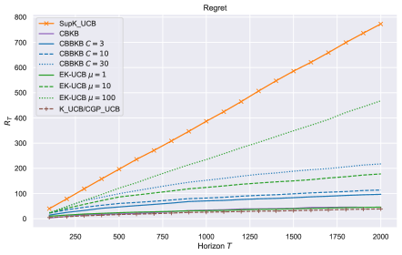
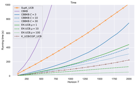
Figure 1: ’Bump’ setting: Regret and running times of EK-UCB, CBBKB, CBKB, SupKUCB and K-UCB, with $T=1000$ and $\lambda=10$ (see Corollary 3.1 and 4.1). EK-UCB matches the best theoretical regret-time compromise when the projection parameter $\mu=\lambda$. We show other values of $\mu$: higher $\mu$ ($\mu=100$) leads to faster computational time but worse regret, and reciprocally ($\mu=1$) leads to worse computational time and better regret. Additional results where $\lambda$ and $\mu$ change simultaneously are available in the Appendix F.

The proof is postponed to Appendix C. In a practical setting, the dictionary size is controlled by the choice of the projection parameter $\mu$. When $\mu$ is too high, it induces a smaller dictionary size $m$ but thus linear regret as indicated in the previous corollary. However, by choosing a low $\mu$, we still recover the original regret but increase the size of the dictionary and thus pay a higher computation time. To recover the original regret, the regularization parameter $\lambda$ must be set to $\mu$ in all cases to recover the original regret, and both values have a theoretical optimal value which depends on the horizon to recover the best convergence rate under the capacity condition assumption.

5 Numerical Experiments

We now evaluate our proposed EK-UCB approach empirically on a synthetic scenario, in order to illustrate its performance in practice. All algorithms have been carefully optimized for fair comparisons. More experimental details, discussions, and additional experimental results are provided in Appendix F.

Experimental setup.

We consider a ’Bump’ synthetic environment with contexts uniformly distributed in $[0,1]^{p}$, with $p=5$, and actions in $[0,1]$. The rewards are generated using the function $r(x,a)=\max(0,1-\|a-a^{*}\|_{1}-\langle w^{*},x-x^{*}\rangle)$ for some $a^{*},w^{*}$ and $x^{*}$ picked randomly and fixed. We also consider additional 2D synthetic settings ’Chessboard’ and ’Step Diagonal’ presented in Appendix F.2.2. We use a Gaussian kernel in this setting. We run our algorithms for $T=2000$ steps and average our results over different 3 random runs.

Baselines.

In our experiments, we chose to compare to K-UCB, SupK-UCB and to works which focus on improving the $\mathcal{O}(T^{3})$ time-complexity for the kernel case. We implemented K-UCB, SupK-UCB (SupKernelUCB, Valko et al. (2013)), EK-UCB (our efficient version of the K-UCB algorithm) as well as our contextual adaptation of the BKB (Calandriello et al., 2019) and BBKB (Calandriello et al., 2020) algorithms; we will refer to these respectively as CBKB and CBBKB. Specifically, we use the same accumulation criteria as Calandriello et al. (2020) for the “resparsification” strategies (i.e., the resampling of the dictionary) with a threshold parameter $C$. We also proceed to the same sampling and equation updates as the original algorithms while using our joint kernel on context-action pairs. Note also that CGP-UCB/K-UCB only differ from their parameter $\beta_{t}$ and match the same algorithm in our implementation (see second last paragraph in Sec. 4.3).

Figure 2: ’Chessboard’ setting: Regret and running times of EK-UCB ($\lambda=\mu$), CBBKB ($C=10$) and CBKB, with $T=2000$ and with varying $\lambda$. We notice that low $\lambda$ values have better regrets but higher computatinal times. Overall EK-UCB achieves the best regret-time compromise for all parameters of $\lambda$ while CBBKB sometimes improves upon the K-UCB complexity but has both higher regret than EK-UCB and higher computational time.

Results.

We report the average regret and running times of the algorithms over different runs in Fig. 1 and Fig. 2 to analyze how the the different algorithms perform. In particular, our algorithm (EK-UCB) achieves low regret while running in low computational time.

In the first example for the ’Bump’ environment in Fig. 1, for $T=2000$, we have set $\lambda~{}=~{}10$ (of the order of $\sqrt{T}$) and see that the value of $\mu=\lambda$ indeed achieves a good tradeoff between regret and time. The parameter $\mu$ determines the quality of the projection required in the algorithm. Thus, for a smaller $\mu$, the algorithm achieves a better regret but pays a higher time complexity. We note that a similar role is played by the parameter $C$ in the BBKB algorithm. The smaller $C$, the more frequent the dictionary updates, and thus the slower is the algorithm. While the CGP-UCB/K-UCB obtains the best regret, we note also, that EK-UCB ($\mu=1$), CBKB (which is CBBKB with $C=1$) essentially take the full dictionary $m\approx T$ and thus also match K-UCB, but with dictionary building computational overheads which make them more computationally intensive than K-UCB itself. In the Appendix F we provide additional results that show that consistently EK-UCB provides the best time-regret compromise with regards to K-UCB.

Second, in Fig. 2 we show for the ’Chessboard’ setting the influence of varying $\lambda$ for all methods (fixing $\mu=\lambda$ for EK-UCB). Both CBBKB and EK-UCB improve upon the K-UCB computational time in this case, but EK-UCB achieves lower computational times while also having lower regrets than CBBKB for all settings. We also notice that the CBKB algorithm runs much slower than the CBBKB algorithm in all experiments, as expected due to its costly dictionary update at every round which requires processing all previous points. The computational overheads of its dictionary building therefore makes it not practical despite its theoretical guarantees. Note also that CBBKB uses scores based on the variance estimates on past states for its “resparfication” strategy and EK-UCB uses leverage scores to build its dictionary thus looking for directions that are orthogonal to the previous anchor points; both approaches are more effective than updating the dictionary at each round. Eventually, recall that our incremental projection scheme allows us to perform rank-one updates of the dictionary. This also contributes to the practical speedup of our EK-UCB algorithm, as compared to the CBBKB strategy.

Moreover, SupK-UCB performs poorly in our experiments due to its over-exploring elimination strategy that might be beneficial only for large $T$ and makes it unpractical in its current time-complexity. Note that the main author of SupK-UCB co-authored Calandriello et al. (2019) where it is mentioned that it indeed has "tighter analysis than GP-UCB [but] does not work well in practice".

6 Discussions

In this work, we proposed a method for contextual kernel UCB algorithms in large-scale problems. The EK-UCB algorithm runs in $\mathcal{O}(Td_{\mathrm{eff}})$ space and $\mathcal{O}(CTd_{\mathrm{eff}}^{2})$ time complexity, which significantly improves over the standard contextual kernel UCB method. Note that while previous efficient Gaussian process algorithms allow to scale up the learning problems in non contextual and discrete action environments, we have shown how the incremental projection updates were crucial to perform efficient approximations in the joint context-action space, providing the same regret guarantees for a smaller computational cost. We note that the batching strategy of BBKB may still be useful even under our incremental updates, and thus provides an interesting avenue for future work. Another natural question is whether we may obtain algorithms with better regret guarantees similar to Valko et al. (2013) in the finite action case, while also achieving gains in computational efficiency as in our work.

Acknowledgments

JM was supported by the ERC grant number 714381 (SOLARIS project) and by ANR 3IA MIAI@Grenoble Alpes, (ANR-19-P3IA-0003).

 

Appendix

 

This appendix is organized as follows:

• Appendix A: summary of the notations used in the analysis

• Appendix B: proofs of Section 3 – Kernel-UCB

• Appendix C: proofs of Section 4 – Efficient Kernel-UCB

• Appendix E: details on the implementation of the algorithms

• Appendix F: additional experiment details, discussions and results

Appendix A List of notations

In this appendix, we recall useful notations that are used throughout the paper.

Below are generic notations and notations related to RKHS:

• $[n]\vcentcolon=\{1,\dots,n\}$

• $\lesssim$ denotes an approximate inequality up to logarithmic multiplicative or additive terms

• $\mathcal{X}$ is the input space

• $\mathcal{A}$ is the action set

• $k:(\mathcal{X}\times\mathcal{A})\times(\mathcal{X}\times\mathcal{A})\to\mathbb{R}$ is a bounded positive definite Kernel

• $\kappa>0$ is an upper-bound on the kernel $\kappa^{2}\geq\sup_{s\in\mathcal{X}\times\mathcal{A}}k(s,s)$.

• $\mathcal{H}$ is the reproducing kernel Hilbert space associated to $k$

• $\phi:\mathcal{X}\times\mathcal{A}\to\mathcal{H}$ is the feature map such that $k(s,s^{\prime})=\langle\phi(s),\phi(s^{\prime})\rangle$ for any $s,s^{\prime}\in\mathcal{X}\times\mathcal{A}$

• $\langle\varphi,\varphi^{\prime}\rangle\vcentcolon=\varphi^{\top}\varphi^{\prime}$ denotes the inner product for any $\varphi,\varphi^{\prime}\in\mathcal{H}$

• $\|\cdot\|$ denotes the norm associated to $\mathcal{H}$. It is the one induced by the inner product, i.e., $\|\varphi\|^{2}=\left<\varphi,\varphi\right>$

• $\|\cdot\|_{V}$ denotes for any symmetric positive semi-definite operator $V:\mathcal{H}\to\mathcal{H}$ the norm such that $\|\varphi\|_{V}=\|V^{1/2}\varphi\|$ for all $\varphi\in\mathcal{H}$

• $L\preccurlyeq L^{\prime}$ means that $L-L^{\prime}$ is positive semi-definite for two operators $L,L^{\prime}$ on $\mathcal{H}$

• $\varphi\otimes\varphi^{\prime}:\mathcal{H}\to\mathcal{H}$ is the tensor product of $\varphi$ and $\varphi^{\prime}\in\mathcal{H}$

Below are notations related to the sequential setting. Here, $t\in[T]$ denotes the index of the round:

• $\theta^{*}\in\mathcal{H}$ is the unknown parameter

• $x_{t}\in\mathcal{X},a_{t}\in\mathcal{A}$ are the context and action played at round $t$

• $s_{t}\vcentcolon=(x_{t},a_{t})\in\mathcal{X}\times\mathcal{A}$

• $\mathcal{S}_{t}\vcentcolon=\{s_{1},\dots,s_{t}\}$ denotes the history

• $\varepsilon_{1},\dots,\varepsilon_{T}$ are independent centered sub-Gaussian noise

• $H_{t}\vcentcolon=(\varepsilon_{1},\dots,\varepsilon_{t})^{\top}$

• $\mathcal{F}_{t}\vcentcolon=\sigma(\varepsilon_{1},\dots,\varepsilon_{t})$ is the natural filtration with respect to $(\varepsilon_{i})_{i\geq 1}$

• $r_{t}\vcentcolon=\langle\theta^{*},\phi(x_{t},a_{t})\rangle+\varepsilon_{t}$ is the reward

• $Y_{t}\vcentcolon=(r_{1},\dots,r_{t})^{\top}\in\mathbb{R}^{t}$ is the vector of rewards

• $\varphi_{t}\vcentcolon=\phi(x_{t},a_{t})\in\mathcal{H}$

• $\lambda>0$ is the regularization parameter

• $F_{t}\vcentcolon=\sum_{s=1}^{t}\varphi_{s}\otimes\varphi_{s}$ is the covariance operator

• $V_{t}\vcentcolon=\sum_{s=1}^{t}\varphi_{s}\otimes\varphi_{s}+\lambda I:\mathcal{H}\to\mathcal{H}$ is the regularized covariance operator

• $\Phi_{t}:\mathcal{H}\to\mathbb{R}^{t}$ is the operator such that $[\Phi_{t}\varphi]_{i}=\varphi(x_{i},a_{i})=\langle\varphi,\phi(x_{i},a_{i})\rangle$ for any $\varphi\in\mathcal{H}$ and $i\in[t]$

• $\Phi^{*}$ denotes the conjugate transpose of a linear operator $\Phi$ on $\mathcal{H}$

• $K_{t}\vcentcolon=\Phi_{t}\Phi_{t}^{*}:\mathbb{R}^{t}\to\mathbb{R}^{t}$ is the kernel matrix at time $t\geq 1$. Note that $[K_{t}]_{ij}=k((x_{i},a_{i}),(x_{j},a_{j}))$.

• $\lambda_{i}(K_{t})$ is the $i$-th largest eigenvalue of $K_{t}$

• $d_{\mathrm{eff}}(\lambda,t)\vcentcolon=\operatorname{Tr}(K_{t}(K_{t}+\lambda I_{t})^{-1})$ is the effective dimension of the matrix $K_{t}$

Below are notations related to the Kernel-UCB algorithm without projections:

• $\hat{\theta}_{t}\vcentcolon=V_{t}^{-1}\Phi_{t}^{*}Y_{t}$ is the estimator of the algorithm

• $\delta>0$ is the confidence level

• $\beta_{t}(\delta)$ is the radius of the confidence ellipsoid of the algorithm

• $\mathcal{C}_{t}\vcentcolon=\big{\{}\theta\in\mathcal{H}:\big{\|}\theta-\hat{\theta}_{t-1}\big{\|}_{V_{t-1}}\leq\beta_{t}(\delta)\big{\}}$ is the confidence ellipsoid played by the algorithm

Below are notations related to the Kernel-UCB algorithm with projections. All along the analysis, the notation $\tilde{x}$ corresponds to the projected version of the object $x$.

• $\mathcal{Z}_{t}\subset\big{\{}(x_{1},a_{1}),\dots,(x_{t},a_{t})\big{\}}$ is a dictionary

• $\tilde{\mathcal{H}}_{t}\vcentcolon=\mathrm{Span}\big{\{}\phi(s),s\in\mathcal{Z}_{t}\big{\}}$ is a linear subspace of $\mathcal{H}$ and is used at round $t$.

• $P_{t}:\mathcal{H}\to\tilde{\mathcal{H}}_{t}$ is the Euclidean projection onto $\mathcal{H}$ so that $\tilde{\mathcal{H}}_{t}=\{P_{t}\varphi,\varphi\in\mathcal{H}\}$

• $\tilde{V}_{t}\vcentcolon=\sum_{s=1}^{t}(P_{t}\varphi_{s})\otimes(P_{t}\varphi_{s})+\lambda I=P_{t}F_{t}P_{t}+\lambda I$ is the regularized projected covariance operator

• $\tilde{\theta}_{t}\vcentcolon=P_{t}\tilde{V}_{t}^{-1}P_{t}\Phi_{t}^{*}Y_{t}$ is the projected estimator of the algorithm

• $\tilde{C}_{t}\vcentcolon=\big{\{}\theta\in\mathcal{H}:\|\theta-\tilde{\theta}_{t-1}\|_{\tilde{V}_{t-1}}\leq\tilde{\beta}_{t}(\delta)\big{\}}$ is the confidence ellipsoid related to the projected estimator

• $\smash{\mu_{t}\vcentcolon=\big{\|}(I-P_{t})F_{t}^{1/2}\big{\|}}^{2}$ is the approximation error of the projection

Eventually, we provide notations related to the kernel matrix computations when we write the update rules of the efficient algorithm.

• $K_{\mathcal{S}}(s^{\prime})$ is the kernel column vector $[k(s_{1},s^{\prime}),\dots,k(s_{l},s^{\prime})]^{\top}$ of size $|\mathcal{S}|=l$. Note that $K_{\mathcal{S}_{t}}(s)=\Phi_{t}\phi(s)$ .

• $K_{\mathcal{Z}\mathcal{S}}$ is the kernel matrix vector $[k(z,s)]_{z\in\mathcal{Z},s\in\mathcal{S}}$ of size $|\mathcal{Z}|\times|\mathcal{S}|$.

• $s_{t,a}=(x_{t},a)$ refers to the pair of context $x_{t}$ and any action $a\in\mathcal{A}_{t}$ that can be chosen in the UCB rule.

Appendix B Proofs of Section 3: Kernel UCB

In this appendix we prove of Lemma 8 and Theorem 3.1.

B.1 Proof of Lemma 8

We first prove Lemma 8, which controls the size of the confidence intervals considered by the algorithm. It states that with probability $1-\delta$, for all $t\geq 1$:

$$\theta^{*}\in C_{t},\quad\text{ where }\quad C_{t}=\big{\{}\theta\in\mathbb{R}^{d},\|\theta-\hat{\theta}_{t-1}\|_{V_{t-1}}\leq\beta_{t}(\delta)\big{\}}\,.$$ (14)

Lemma 8.

Let $\delta\in(0,1)$. Assume $\kappa^{2}\geq\sup_{s\in\mathcal{X}\times\mathcal{A}}k(s,s)$. Then with probability at least $1-T\delta$, for all $t\in[T]$

$$\|\hat{\theta}_{t}-\theta^{*}\|_{V_{t}} \leq\sqrt{\lambda}\|\theta^{*}\|+\sqrt{2\log\frac{1}{\delta}+\log\left(\det\left(\frac{1}{\lambda}(K_{t}+\lambda I)\right)\right)}$$

$$\leq\sqrt{\lambda}\|\theta^{*}\|+\sqrt{2\log\frac{1}{\delta}+\log\left(e+\dfrac{et\kappa^{2}}{\lambda}\right)d_{\mathrm{eff}}(\lambda,T)}\quad=\vcentcolon\quad\beta_{t+1}(\delta).$$

Proof.

The analysis is inspired by the one of Abbasi-yadkori et al. (2011) for linear bandits and uses inequality tails on vector valued martingales. We introduce $M_{t}=\sum_{s=1}^{t}\varphi_{s}\varepsilon_{s}\in\mathcal{H}$, which is a martingale with regards to the natural filtration $\mathcal{F}_{t}\vcentcolon=\sigma(\varepsilon_{1},\dots,\varepsilon_{t})$. Solving the least-square optimization problem (4), $\hat{\theta}_{t}$ equals

$$\hat{\theta_{t}}=V_{t}^{-1}\sum_{s=1}^{t}\varphi_{s}Y_{s}=V_{t}^{-1}\sum_{s=1}^{t}\varphi_{s}(\varphi_{s}^{\top}\theta^{*}+\varepsilon_{s})=V_{t}^{-1}{\left((V_{t}-\lambda I_{d})\theta^{*}+M_{t}\right)}=\theta^{*}-\lambda V_{t}^{-1}\theta^{*}+V_{t}^{-1}M_{t}\,.$$

Multiplying by the square root of $V_{t}$ and using the triangle inequality

$$\Big{\|}V_{t}^{1/2}\big{(}\hat{\theta}_{t}-\theta^{*}\big{)}\Big{\|}=\Big{\|}-\lambda V_{t}^{-1/2}\theta^{*}+V_{t}^{-1/2}M_{t}\Big{\|}\leq\lambda\big{\|}V_{t}^{-1/2}\theta^{*}\big{\|}+\big{\|}V_{t}^{-1/2}M_{t}\big{\|}\,.$$

On the other hand, given that $V_{t}=F_{t}+\lambda I$ where $F_{t}$ is positive semi-definite, $V_{t}^{-1/2}\preccurlyeq\lambda^{-1/2}I$ and thus

$$\lambda\|V_{t}^{-1/2}\theta^{*}\|\leq\lambda\frac{1}{\sqrt{\lambda}}\|\theta^{*}\|=\sqrt{\lambda}\|\theta^{*}\|\,.$$

We now prove for the other term that with probability at least $1-\delta$

$$\|V_{t}^{-1/2}M_{t}\|\leq\sqrt{2\log\frac{1}{\delta}+\log\det\frac{1}{\lambda}(K_{t}+\lambda I)}\,.$$

Step 1: Martingales For all $\nu\in\mathcal{H}$, we define the random-variable

$$S_{t,\nu}=\exp\Big{(}\nu^{\top}M_{t}-\frac{1}{2}\nu^{\top}V_{t}\nu\Big{)}$$

and now show that it is a $\mathcal{F}_{t}$-super-martingale. First, note that the common distribution of the $\varepsilon_{1},\dots,\varepsilon_{t}$ is 1-sub Gaussian, i.e., for all $\mathcal{F}_{t-1}$-measurable real-valued random variable $\nu_{t-1}$, we have

$$\operatorname{\mathbb{E}}\big{[}\exp(\nu_{t-1}\varepsilon_{t})|\mathcal{F}_{t-1}\big{]}\leq\exp\Big{(}\frac{\nu_{t-1}^{2}}{2}\Big{)}\,.$$ (15)

Thus, using that $M_{t}=M_{t-1}+\varphi_{t}\varepsilon_{t}$ and $V_{t}=V_{t-1}+\varphi_{t}\otimes\varphi_{t}$,

$$\operatorname{\mathbb{E}}\left[S_{t,\nu}|\mathcal{F}_{t-1}\right] =\operatorname{\mathbb{E}}\Big{[}\exp\big{(}\nu^{\top}M_{t}-\frac{1}{2}\nu^{\top}V_{t}\nu\big{)}|\mathcal{F}_{t-1}\Big{]}$$

$$=\operatorname{\mathbb{E}}\Big{[}S_{t-1,\nu}\exp\big{(}\nu^{\top}\varphi_{t}\varepsilon_{t}-\frac{1}{2}\nu^{\top}(\varphi_{t}\otimes\varphi_{t})\nu\big{)}|\mathcal{F}_{t-1}\Big{]}$$

$$=S_{t-1,\nu}\operatorname{\mathbb{E}}\Big{[}\exp\big{(}\nu^{\top}\varphi_{t}\varepsilon_{t}-\frac{1}{2}(\nu^{\top}\varphi_{t})^{2}\big{)}\big{|}\mathcal{F}_{t-1}\Big{]}\leq S_{t-1,\nu}\,,$$

where the last inequality is by applying (15) with $\nu_{t-1}=\nu^{\top}\varphi_{t}$ since $\varphi_{t}=\phi(x_{t},a_{t})$ is $\mathcal{F}_{t-1}$-measurable. Therefore, $S_{t,\nu}$ is a $\mathcal{F}_{t}$-super-martingale for any $\nu\in\mathcal{H}$, and

$$\operatorname{\mathbb{E}}\big{[}S_{t,\nu}\big{]}\leq\operatorname{\mathbb{E}}\big{[}S_{0,\nu}\big{]}=\exp\Big{(}-\frac{\lambda}{2}\|\nu\|^{2}\Big{)}\,.$$ (16)

Rewriting $S_{t,\nu}$ in its vertex form with $m=V_{t-1}M_{t}$ yields

$$S_{t,\nu}=\exp\left(-\frac{1}{2}(\nu-m)^{\top}V_{t}(\nu-m)\right)\times\exp\Big{(}\frac{1}{2}\big{\|}V_{t}^{-1/2}M_{t}\big{\|}^{2}\Big{)}\,,$$

which substituted into (16) entails

$$\operatorname{\mathbb{E}}\Bigg{[}\exp\Big{(}-\frac{1}{2}(\nu-m)^{\top}V_{t}(\nu-m)\Big{)}\times\exp\Big{(}\frac{1}{2}\big{\|}V_{t}^{-1/2}M_{t}\big{\|}^{2}\Big{)}\bigg{]}\leq\exp\Big{(}-\frac{\lambda}{2}\|\nu\|^{2}\Big{)},\qquad\forall\nu\in\mathcal{H}\,.$$ (17)

Step 2: Laplace’s method integrating

Now, following Laplace’s method which is standard for the proof of LinUCB, the goal is to integrate both sides of the above expression. Let us first rewrite it in order to consider finite dimensional objects thanks to the Kernel trick.

Recalling $V_{t}\vcentcolon=\Phi_{t}^{*}\Phi_{t}+\lambda I$ and $K_{t}\vcentcolon=\Phi_{t}\Phi_{t}^{*}$, following (Valko et al., 2013), we will use the following identities:

$$(\Phi_{t}^{*}\Phi_{t}+\lambda I)\Phi_{t}^{*} =\Phi_{t}^{*}(\Phi_{t}\Phi_{t}^{*}+\lambda I)$$ (18)

$$\Rightarrow\hskip 64.87224ptV_{t}\Phi_{t}^{*} =\Phi_{t}^{*}(K_{t}+\lambda I)$$ (19)

$$\Rightarrow\qquad\Phi_{t}^{*}(K_{t}+\lambda I)^{-1} =V_{t}^{-1}\Phi_{t}^{*}\,.$$ (20)

Let $x\in\mathbb{R}^{t}$ and write $\nu=V_{t}^{-1}\Phi_{t}^{*}x\in\mathcal{H}$ and recall that $m=V_{t}^{-1}M_{t}=V_{t}^{-1}\Phi_{t}^{*}H_{t}$, where $H_{t}=(\varepsilon_{1},\dots,\varepsilon_{t})^{\top}$. We have

$$\exp\Big{(}-\frac{1}{2}(\nu-m)^{\top}V_{t} (\nu-m)\Big{)}=\exp\Big{(}-\frac{1}{2}(x-H_{t})^{\top}\Phi_{t}V_{t}^{-1}V_{t}V_{t}^{-1}\Phi_{t}^{*}(x-H_{t})\Big{)}$$

$$=\exp\Big{(}-\frac{1}{2}(x-H_{t})^{\top}\Phi_{t}\Phi_{t}^{*}(K_{t}+\lambda I)^{-1}(x-H_{t})\Big{)}\qquad\leftarrow\text{ by~{}\eqref{eq:kerneltrick3}}$$

$$=\exp\Big{(}-\frac{1}{2}(x-H_{t})^{\top}K_{t}(K_{t}+\lambda I)^{-1}(x-H_{t})\Big{)}\hskip 31.2982pt\leftarrow K_{t}=\Phi_{t}\Phi_{t}^{*}$$

$$=\exp\Big{(}-\frac{1}{2}(x-H_{t})^{\top}K_{t}^{1/2}(K_{t}+\lambda I)^{-1}K_{t}^{1/2}(x-H_{t})\Big{)}\,,$$ (21)

where the last equality is because $(K_{t}+\lambda I)^{-1}$ and $K_{t}^{1/2}$ commute. Similarly,

$$\exp\Big{(}-\frac{\lambda}{2}\|\nu\|^{2}\Big{)}=\exp\Big{(}-\frac{\lambda}{2}x^{\top}K_{t}^{1/2}(K_{t}+\lambda I)^{-2}K_{t}^{1/2}x\Big{)}\,.$$

Combining with (16) and (21) thus gives for any $x\in\mathbb{R}^{t}$,

$$\operatorname{\mathbb{E}}\bigg{[}\exp\Big{(}-\frac{1}{2}(x-H_{t})^{\top}K_{t}^{1/2}(K_{t}+\lambda I)^{-1}K_{t}^{1/2}(x-H_{t})\Big{)}\times\exp\Big{(}\frac{1}{2}\big{\|}V_{t}^{-1/2}M_{t}\big{\|}^{2}\Big{)}\bigg{]}\\ \leq\exp\Big{(}-\frac{\lambda}{2}x^{\top}K_{t}^{1/2}(K_{t}+\lambda I)^{-2}K_{t}^{1/2}x\Big{)}\,.$$ (22)

Now, that we are back to finite dimensional space, the idea would consists in integrating both parts over $x\in\mathbb{R}^{t}$. But the matrix $K_{t}$ may be non-invertible, we thus need a few more steps to integrate over $\mathrm{Im}(K_{t})$ only.

Let $d_{t}=\mathrm{rank}(K_{t})$ and $Q_{t}\in\mathbb{R}^{t\times d_{t}}$ the matrix formed by the orthonormal eigenvectors of $K_{t}$ with non-zero eigenvalues. Let $u\in\mathbb{R}^{d_{t}}$ then $Q_{t}u\in\mathrm{Im}(K_{t})$ and there exists $x\in\mathbb{R}^{t}$ such that $K_{t}^{1/2}x=Q_{t}u$. Defining $z\in\mathbb{R}^{d_{t}}$ such that $Q_{t}z=K_{t}^{1/2}H_{t}$ and substituting into Inequality (22) yields, for any $u\in\mathbb{R}^{d_{t}}$

$$\operatorname{\mathbb{E}}\bigg{[}\exp\Big{(}-\frac{1}{2}(u-z)^{\top}Q_{t}^{\top}(K_{t}+\lambda I)^{-1}Q_{t}(u-z)\Big{)}\times\exp\Big{(}\frac{1}{2}\big{\|}V_{t}^{-1/2}M_{t}\big{\|}^{2}\Big{)}\bigg{]}\\ \leq\exp\Big{(}-\frac{\lambda}{2}u^{\top}Q_{t}^{\top}(K_{t}+\lambda I)^{-2}Q_{t}u\Big{)}\,.$$ (23)

Now, we integrate both sides over $u\in\mathbb{R}^{d_{t}}$, recognizing a multidimensional Gaussian density, we have

$$\int_{\mathbb{R}^{d}}\exp\Big{(}-\frac{1}{2}(u-z)^{\top}Q_{t}^{\top}(K_{t}+\lambda I)^{-1}Q_{t}(u-z)\Big{)}d\mu(u)=\sqrt{\det\big{(}2\pi(Q_{t}^{\top}(K_{t}+\lambda I)^{-1}Q_{t})^{-1}\big{)}}\\ =\sqrt{(2\pi)^{d_{t}}\prod_{i=1}^{d_{t}}\big{(}\lambda_{i}(K_{t})+\lambda\big{)}}\,,$$

where $\lambda_{i}(K_{t})$ is the $i$-th largest eigenvalue of $K_{t}$. Similarly

$$\int_{\mathbb{R}^{d}}\exp\Big{(}-\frac{\lambda}{2}u^{\top}Q_{t}^{\top}(K_{t}+\lambda I)^{-2}Q_{t}u\Big{)}d\mu(u)=\sqrt{\det\Big{(}2\pi\lambda^{-1}\big{(}Q_{t}^{\top}(K_{t}+\lambda I)^{-2}Q_{t}\big{)}^{-1}\Big{)}}=\sqrt{\Big{(}\frac{2\pi}{\lambda}\Big{)}^{d_{t}}\prod_{i=1}^{d_{t}}\big{(}\lambda_{i}(K_{t})+\lambda\big{)}^{2}}\,.$$

Therefore, by the Fubini-Tonelli theorem, plugging the last two equations into Inequality (23) entails

$$\sqrt{(2\pi)^{d_{t}}\prod_{i=1}^{d_{t}}\big{(}\lambda_{i}(K_{t})+\lambda\big{)}}\operatorname{\mathbb{E}}\bigg{[}\exp\Big{(}\frac{1}{2}\big{\|}V_{t}^{-1/2}M_{t}\big{\|}^{2}\Big{)}\bigg{]}\leq\sqrt{\Big{(}\frac{2\pi}{\lambda}\Big{)}^{d_{t}}\prod_{i=1}^{d_{t}}\big{(}\lambda_{i}(K_{t})+\lambda\big{)}^{2}}\,,$$

which, after reorganizing the terms, yields

$$\operatorname{\mathbb{E}}\bigg{[}\exp\Big{(}\frac{1}{2}\big{\|}V_{t}^{-1/2}M_{t}\big{\|}^{2}\Big{)}\bigg{]}\leq\sqrt{\prod_{i=1}^{d_{t}}\Big{(}1+\frac{\lambda_{i}(K_{t})}{\lambda}\Big{)}}=\sqrt{\frac{\det(K_{t}+\lambda I)}{\lambda^{t}}}\,.$$

Step 3: Markov-Chernov bound. It remains to upper-bound the above expectation using concentration inequalities. For $u>0$,

$$P\left(\|V_{t}^{-1/2}M_{t}\|>u\right)=P\left(\dfrac{\|V_{t}^{-1/2}M_{t}\|^{2}}{2}>\dfrac{u^{2}}{2}\right) \leq\exp\left(-\frac{1}{2}u^{2}\right)\displaystyle\operatorname{\mathbb{E}}\left[\exp\left(\frac{1}{2}\|V_{t}^{-1/2}M_{t}\|^{2}\right)\right]$$

$$\leq\exp\left(-\dfrac{u^{2}}{2}+\dfrac{1}{2}\log\dfrac{\det(K_{t}+\lambda I)}{\lambda^{t}}\right)=\delta$$ (24)

for the claimed choice

$$u=\sqrt{2\log\frac{1}{\delta}+\log\det\frac{1}{\lambda}(K_{t}+\lambda I)}\,.$$

The proof then concludes by using Prop. 3.1 on the $\log\det\frac{1}{\lambda}(K_{t}+\lambda I)$ term and by applying a union bound. ∎

B.2 Proof of Theorem 3.1

We are now ready to prove Theorem 3.1, which upper-bounds the regret of K-UCB.

Theorem 3.1.

Let $T\geq 2$ and $\theta^{*}\in\mathcal{H}$. Assume that $|\langle\phi(x,a),\theta^{*}\rangle|\leq 1$ and $\|\phi(x,a)\|\leq\kappa$ for all $a\in\bigcup_{t=1}^{T}\mathcal{A}_{t}\subset\mathcal{A}$ and $x\in\mathcal{X}$. Then, the K-UCB rule defined in Eq. (3) for the choice $\mathcal{C}_{t}$ as in (5) satisfies the pseudo-regret bound

$$R_{T} \leq 2+2\sqrt{T\left(\log\left(e+\dfrac{eT\kappa^{2}}{\lambda}\right)d_{\mathrm{eff}}(\lambda,T)\right)}\left[\sqrt{\lambda}\|\theta^{*}\|+\sqrt{2\log(T)+\log\left(e+\dfrac{eT\kappa^{2}}{\lambda}\right)d_{\mathrm{eff}}(\lambda)}\right]$$

$$\lesssim\sqrt{T}\Big{(}\|\theta^{*}\|\sqrt{\lambda d_{\mathrm{eff}}(\lambda,T)}+d_{\mathrm{eff}}(\lambda,T)\Big{)}\,.$$

Proof.

Let $\delta\in(0,1/2)$. By Lemma 8, with probability $1-T\delta$,

$$\forall t\in[T],\quad\theta^{*}\in C_{t}\,.$$ (25)

Step 1: Small instantaneous regrets under the event (25). Assume that (25) holds. Let

$$a_{t}^{*}\vcentcolon=\max_{a\in\mathcal{A}_{t}}\langle\phi(x_{t},a),\theta^{*}\rangle\quad\text{and}\quad\Delta_{t}\vcentcolon=\langle\phi(x_{t},a_{t}^{*})-\phi(x_{t},a_{t}),\theta^{*}\rangle$$

be respectively the optimal decision and the instantaneous regret at round t. We also define

$$\rho_{t}\in\operatorname*{arg\,max}_{\theta\in C_{t}}\big{\{}\langle\phi(x_{t},a_{t}),\theta\rangle\big{\}}\,.$$

Since $\theta^{*}\in C_{t}$, we have

$$\langle\phi(x_{t},a_{t}^{*}),\theta^{*}\rangle\leq\max_{\theta\in C_{t}}\{\langle\phi(x_{t},a_{t}^{*}),\theta\rangle\}=\text{K-UCB}_{t}(a_{t}^{*})\leq\text{K-UCB}_{t}(a_{t})=\max_{\theta\in C_{t}}\{\langle\phi(x_{t},a_{t}),\theta\rangle\}=\langle\phi(x_{t},a_{t}),\rho_{t}\rangle\,,$$

which entails because $\theta^{*}$ and $\tilde{\theta}_{t-1}$ belong to $C_{t}$,

$$\Delta_{t}=\langle\phi(x_{t},a_{t}^{*})-\phi(x_{t},a_{t}),\theta^{*}\rangle\leq\langle\phi(x_{t},a_{t}),\rho_{t}-\theta^{*}\rangle\leq\|\phi(x_{t},a_{t})\|_{V_{t-1}^{-1}}\|\rho_{t}-\theta^{*}\|_{V_{t-1}}\leq 2\|\phi(x_{t},a_{t})\|_{V_{t-1}^{-1}}\beta_{t}(\delta)\,.$$

Recall that $\varphi_{t}\vcentcolon=\phi(x_{t},a_{t})$. Then, summing over $t=1,\dots,T$ and using that by assumption

$$|\Delta_{t}|\leq\big{|}\langle\phi(x_{t},a_{t}^{*}),\theta^{*}\rangle\big{|}+\big{|}\langle\phi(x_{t},a_{t}),\theta^{*}\rangle\big{|}\leq 2\sup_{x\in\mathcal{X},a\in\mathcal{A}_{t}}|\langle\phi(x,a),\theta^{*}\rangle|\leq 2\,,$$

we can write the cumulative regret as

$$\sum_{t=1}^{T}\Delta_{t} \textstyle\leq\sqrt{T\sum_{t=1}^{T}\Delta_{t}^{2}}\hskip 108.12054pt\leftarrow\quad\text{Jensen's inequality}$$

$$\textstyle\leq 2\sqrt{T\sum_{t=1}^{T}\min\{\|\varphi_{t}\|_{V_{t-1}^{-1}}^{2}\beta_{t}(\delta)^{2},1\}}$$

$$\textstyle\leq 2\beta_{T}(\delta)\sqrt{T\sum_{t=1}^{T}\min\{\|\varphi_{t}\|_{V_{t-1}^{-1}}^{2},1\}}\hskip 10.81218pt\leftarrow\quad 1\leq\beta_{t}(\delta)\leq\beta_{T}(\delta)$$

$$\textstyle\leq 2\beta_{T}(\delta)\sqrt{T\sum_{t=1}^{T}\log\Big{(}1+\|\varphi_{t}\|_{V_{t-1}^{-1}}^{2}\Big{)}}\hskip 5.69046pt\leftarrow\quad\min(u,1)\leq 2\log(1+u),\ \forall u>0\,.$$ (26)

Now we will use the kernel trick to obtain a formulation of $\varphi_{t}^{\top}V_{t-1}^{-1}\varphi_{t}$ using gram matrices. Define $s_{t}:=(x_{t},a_{t})$ and $\mathcal{S}_{t}:=(s_{i})_{1\leq i\leq t}$ the historical data. For any $l\geq 1$ and $\mathcal{S}\in(\mathcal{X}\times\mathcal{A})^{l}$, we also denote by $K_{\mathcal{S}}(s^{\prime})$ the kernel column vector $[k(s_{1},s^{\prime}),\dots,k(s_{l},s^{\prime})]^{\top}$ of size $|\mathcal{S}|=l$. Specifically, we have $K_{\mathcal{S}_{t-1}}(s_{t}):=[k(s_{1},s_{t}),\dots,k(s_{t-1},s_{t})]^{\top}=\Phi_{t-1}\varphi_{t}\in\mathbb{R}^{t}$. When multiplying $V_{t-1}\vcentcolon=\Phi_{t-1}^{*}\Phi_{t-1}+\lambda I$ by $\varphi_{t}$ on the right, we can express

$$V_{t-1}\varphi_{t} =\Phi_{t-1}^{*}K_{\mathcal{S}_{t-1}}\left(s_{t}\right)+\lambda\varphi_{t},$$

$$\Rightarrow\hskip 28.45274pt\varphi_{t} =V_{t-1}^{-1}\Phi_{t-1}^{*}K_{\mathcal{S}_{t-1}}\left(s_{t}\right)+\lambda V_{t-1}^{-1}\varphi_{t}$$

$$\Rightarrow\hskip 28.45274pt\varphi_{t} =\Phi_{t-1}^{*}(K_{t-1}+\lambda I)^{-1}K_{\mathcal{S}_{t-1}}\left(s_{t}\right)+\lambda V_{t-1}^{-1}\varphi_{t}\,,$$

where the last equation is by Eq. (20). Thus, multiplying now by $\varphi_{t}^{\top}$ on the left and using $\varphi_{t}^{\top}\Phi_{t-1}^{*}=K_{\mathcal{S}_{t-1}}(s_{t})$ entails

$$\varphi_{t}^{\top}\varphi_{t} =K_{\mathcal{S}_{t-1}}\left(s_{t}\right)^{\top}(K_{t-1}+\lambda I)^{-1}K_{\mathcal{S}_{t-1}}\left(s_{t}\right)+\lambda\varphi_{t}^{\top}V_{t-1}^{-1}\varphi_{t}\,.$$

Therefore, reorganizing the terms ans recognizing $\smash{\|\varphi_{t}\|_{V_{t-1}^{-1}}^{2}=\varphi_{t}^{\top}V_{t-1}^{-1}\varphi_{t}}$ and $\smash{k(s_{t},s_{t})=\varphi_{t}^{\top}\varphi_{t}}$, we can write

$$1+ \|\varphi_{t}\|_{V_{t-1}^{-1}}^{2}=1+\varphi_{t}^{\top}V_{t-1}^{-1}\varphi_{t}$$

$$=\dfrac{\lambda+k(s_{t},s_{t})}{\lambda}-\dfrac{1}{\lambda}K_{\mathcal{S}_{t-1}}(s_{t})^{\top}(K_{t-1}+\lambda I)^{-1}K_{\mathcal{S}_{t-1}}(s_{t})$$

$$=\dfrac{\lambda+k(s_{t},s_{t})}{\lambda}\bigg{(}1-K_{\mathcal{S}_{t-1}}(s_{t})^{\top}(K_{t-1}+\lambda I)^{-1}K_{\mathcal{S}_{t-1}}(s_{t})\big{(}\lambda+k(s_{t},s_{t})\big{)}^{-1}\bigg{)}$$

$$=\dfrac{\lambda+k(s_{t},s_{t})}{\lambda}\det\bigg{(}1-K_{\mathcal{S}_{t-1}}(s_{t})^{\top}(K_{t-1}+\lambda I)^{-1}K_{\mathcal{S}_{t-1}}(s_{t})\big{(}\lambda+k(s_{t},s_{t})\big{)}^{-1}\bigg{)}$$

$$=\dfrac{\lambda+k(s_{t},s_{t})}{\lambda}\det\bigg{(}I-(K_{t-1}+\lambda I)^{-1/2}K_{\mathcal{S}_{t-1}}(s_{t})\big{(}\lambda+k(s_{t},s_{t})\big{)}^{-1}K_{\mathcal{S}_{t-1}}(s_{t})^{\top}(K_{t-1}+\lambda I)^{-1/2}\bigg{)}\,,$$

where the last equality follows by the matrix determinant lemma $\det(I+AB^{\top})=\det(I+B^{\top}A)$ if $A$ and $B$ are $n$-by-$m$ matrices. Then, $1+\|\varphi_{t}\|_{V_{t-1}^{-1}}^{2}$ equals

$$\dfrac{\lambda+k(s_{t},s_{t})}{\lambda}\det\bigg{(}(K_{t-1}+\lambda I)^{-1/2}\Big{(}K_{t-1}+\lambda I-K_{\mathcal{S}_{t-1}}(s_{t})\big{(}\lambda+k(s_{t},s_{t})\big{)}^{-1}K_{\mathcal{S}_{t-1}}(s_{t})^{\top}\Big{)}(K_{t-1}+\lambda I)^{-1/2}\bigg{)}\\ =\dfrac{\lambda+k(s_{t},s_{t})}{\lambda}\dfrac{\det\Big{(}K_{t-1}+\lambda I-K_{\mathcal{S}_{t-1}}(s_{t})\big{(}\lambda+k(s_{t},s_{t})\big{)}^{-1}K_{\mathcal{S}_{t-1}}(s_{t})^{\top}\Big{)}}{\det(K_{t-1}+\lambda I)}\,.$$

Now, using that

$$K_{t}+\lambda I=\begin{bmatrix}K_{t-1}+\lambda I&K_{S_{t-1}}(s_{t})\\ K_{S_{t-1}}(s_{t})^{\top}&k(s_{t},s_{t})+\lambda\end{bmatrix}\,,$$

by the block matrix determinant formula

$$\det\big{(}K_{t}+\lambda I\big{)}=(k(s_{t},s_{t})+\lambda)\det\Big{(}K_{t-1}+\lambda I-K_{S_{t-1}}(s_{t})(k(s_{t},s_{t})+\lambda)^{-1}K_{S_{t-1}}(s_{t})^{\top}\Big{)}$$

we finally get

$$1+\|\varphi_{t}\|_{V_{t-1}^{-1}}^{2}=\dfrac{1}{\lambda}\dfrac{\det(K_{t}+\lambda I)}{\det(K_{t-1}+\lambda I)}\,.$$ (27)

Note here that contrary to the proof in Lattimore and Szepesvári (2020), we used here computations using the gram matrix $K_{t}$ instead of the $V_{t}$ which lives in the feature space that can be infinite dimensional.

Taking the $\log$ and summing over $t=1,\dots,T$ telescopes

$$\sum_{t=1}^{T}\log\left(1+\|\varphi_{t}\|_{V_{t-1}^{-1}}^{2}\right)=\log\left(\det\left(\frac{1}{\lambda}(K_{t}+\lambda I)\right)\right)\leq\log\left(e+\dfrac{eT\kappa^{2}}{\lambda}\right)d_{\mathrm{eff}}(\lambda,T)\,,$$

where we used the Proposition 3.1 for the last inequality and that . Substituting into the regret bound (26) together with $\beta_{T}(\delta)\leq\beta_{T+1}(\delta)$ entails with probability at least $1-T\delta$

$$\sum_{t=1}^{T}\Delta_{t}\leq 2\beta_{T+1}(\delta)\sqrt{T\left(e+\dfrac{eT\kappa^{2}}{\lambda}\right)d_{\mathrm{eff}}(\lambda,T)}\,.$$

Choosing $\delta=1/T^{2}$, taking the expectation $R_{T}=\operatorname{\mathbb{E}}\big{[}\sum_{t=1}^{T}\Delta_{t}\big{]}$ and using $|\Delta_{t}|\leq 2$ concludes. ∎

We now provide a proof for the Corollary that gives out the convergence speed of the K-UCB algorithm with the capacity condition assumption.

B.3 Proof of Corollary 3.1

Corollary 3.1.

Assuming the capacity condition $d_{\mathrm{eff}}\leq(T/\lambda)^{\alpha}$ for $0\leq\alpha\leq 1$, the regret of K-UCB is bounded as $R_{T}\lesssim T^{\frac{1+3\alpha}{2+2\alpha}}$ with an optimal $\lambda\approx T^{\frac{\alpha}{1+\alpha}}$.

Proof.

Starting from $R_{T}\lesssim\sqrt{T}\Big{(}\sqrt{\lambda d_{\mathrm{eff}}(\lambda)}+d_{\mathrm{eff}}(\lambda)\Big{)}$ and assuming the capacity condition $d_{\mathrm{eff}}(\lambda)\lesssim\Big{(}\frac{T}{\lambda}\Big{)}^{\alpha}$ for some $\alpha\in(0,1)$,

$$R_{T}\lesssim\sqrt{T}\Big{(}\sqrt{T^{\alpha}\lambda^{1-\alpha}}+T^{\alpha}\lambda^{-\alpha}\Big{)}\,.$$

Minimizing in $\lambda>0$ entails

$$\sqrt{T^{\alpha}\lambda^{1-\alpha}}=T^{\alpha}\lambda^{-\alpha}\quad\Rightarrow\quad\lambda^{*}=T^{\frac{\alpha}{1+\alpha}}\,,$$

which yields for $\lambda=\lambda^{*}$

$$R_{T}\lesssim T^{\frac{1}{2}+\alpha-\frac{\alpha^{2}}{1+\alpha}}=T^{\frac{1+3\alpha}{2+2\alpha}}\,.$$

∎

Appendix C Proofs of Section 4: Efficient Kernel-UCB

Let us start by recalling the setting and the notation of this section. Let $\mathcal{Z}_{t}\subseteq\mathcal{S}_{t}$, $\smash{\tilde{\mathcal{H}}_{t}\vcentcolon=\mathrm{Span}\big{\{}\phi(s),s\in\mathcal{Z}_{t}\big{\}}}$ be the corresponding linear subspace of $\mathcal{H}$, and $P_{t}:\mathcal{H}\to\tilde{\mathcal{H}}_{t}$ be the Euclidean projection onto $\mathcal{H}$ so that $\smash{\tilde{\mathcal{H}}_{t}=\{P_{t}\varphi,\varphi\in\mathcal{H}\}}$. The EK-UCB algorithm also builds an estimator

$$\tilde{\theta}_{t-1}\in\operatorname*{arg\,min}_{\theta\in\tilde{\mathcal{H}}_{t-1}}\bigg{\{}\sum_{s=1}^{t-1}\left(\langle\theta,\phi(x_{s},a_{s})\rangle-r_{s}\right)^{2}+\lambda\|\theta\|^{2}\bigg{\}}\in{\tilde{\mathcal{H}}}_{t-1}\,,$$ (28)

and uses the confidence set $\smash{\tilde{C}_{t}\vcentcolon=\big{\{}\theta\in\mathcal{H}:\|\theta-\tilde{\theta}_{t-1}\|_{\tilde{V}_{t-1}}\leq\tilde{\beta}_{t}(\delta)\big{\}}}$. We define $\smash{\tilde{V}_{t}\vcentcolon=\sum_{s=1}^{t}(P_{t}\varphi_{s})\otimes(P_{t}\varphi_{s})+\lambda I}$, that we rewrite $\tilde{V}_{t}=P_{t}F_{t}P_{t}+\lambda I$ where $\Phi_{t}^{*}=[\varphi_{1},\dots,\varphi_{t}]$ and $F_{t}=\Phi_{t}^{*}\Phi_{t}$. Recalling the notation, $\smash{Y_{t}\vcentcolon=(r_{1},\dots,r_{t})^{\top}}$, we then obtain that $\smash{\tilde{\theta}_{t}=P_{t}\tilde{V}_{t}^{-1}P_{t}\Phi_{t}^{*}Y_{t}}$. We recall the definition $\smash{\mu_{t}\vcentcolon=\big{\|}(I-P_{t})F_{t}^{1/2}\big{\|}^{2}}$.

C.1 Proof of Lemma 12

The following lemma serves to compute the distance of the center $\tilde{\theta}_{t}$ to any point in the ellipsoid in the projected space $\tilde{\mathcal{H}}_{t}$. Note that the norm uses the geometry induced by the direction matrix $\tilde{V}_{t}$.

Lemma 12.

Let $\delta\in(0,1)$. Assume that $\sup_{s\in\mathcal{X}\times\mathcal{A}}k(s,s)\leq\kappa^{2}$. Then, with probability $1-\delta$, for all $t\geq 1$

$$\|\tilde{\theta}_{t}-\theta^{*}\|_{\tilde{V}_{t}} \leq\left(\sqrt{\lambda}+\sqrt{\mu_{t}}\right)\|\theta^{*}\|+\sqrt{4\log\frac{1}{\delta}+2\log\det\Big{(}\dfrac{{K}_{t}+\lambda I}{\lambda}}\Big{)}$$

$$\leq\left(\sqrt{\lambda}+\sqrt{\mu_{t}}\right)\|\theta^{*}\|+\sqrt{4\log\frac{1}{\delta}+2\log\left(e+\dfrac{et\kappa^{2}}{\lambda}\right)d_{\mathrm{eff}}(\lambda,T)}\quad\vcentcolon=\quad\tilde{\beta}_{t+1}(\delta)\,,$$

where $\|\theta\|_{V}^{2}=\theta^{\top}V\theta$.

Proof.

Let $t\geq 1$. Note that $P_{t}V_{t}P_{t}=P_{t}(F_{t}+\lambda I)P_{t}=P_{t}\tilde{V}_{t}=\tilde{V}_{t}P_{t}$ and consequently as well $P_{t}\tilde{V}_{t}^{-1}=\tilde{V}_{t}^{-1}P_{t}$. We can write with $H_{t}\vcentcolon=(\varepsilon_{1},\dots,\varepsilon_{t})^{\top}$,

$$\tilde{\theta}_{t} =P_{t}\tilde{V}_{t}^{-1}P_{t}\Phi_{t}^{*}Y_{t}$$

$$=\tilde{V}_{t}^{-1}P_{t}\Phi_{t}^{*}Y_{t}\hskip 199.16928pt\leftarrow\quad P_{t}\tilde{V}_{t}^{-1}=\tilde{V}_{t}^{-1}P_{t}$$

$$=\tilde{V}_{t}^{-1}P_{t}\Phi_{t}^{*}(\Phi_{t}\theta^{*}+H_{t})$$

$$=\tilde{V}_{t}^{-1}P_{t}F_{t}P_{t}\theta^{*}+\tilde{V}_{t}^{-1}P_{t}F_{t}(I-P_{t})\theta^{*}+\tilde{V}_{t}^{-1}P_{t}\Phi_{t}^{*}H_{t}$$

$$=\theta^{*}-\lambda\tilde{V}_{t}^{-1}\theta^{*}+\tilde{V}_{t}^{-1}P_{t}F_{t}(I-P_{t})\theta^{*}+\tilde{V}_{t}^{-1}P_{t}\Phi_{t}^{*}H_{t}\,.$$

To obtain later on the norm $\|\tilde{\theta}_{t}-\theta^{*}\|_{\tilde{V}_{t}}$, we multiply by $\tilde{V}_{t}^{1/2}$ on the left

$$\tilde{V}_{t}^{1/2}(\tilde{\theta}_{t}-\theta^{*})=-\underbrace{\lambda\tilde{V}_{t}^{-1/2}\theta^{*}}_{\ref{item1}}+\underbrace{\tilde{V}_{t}^{-1/2}P_{t}F_{t}(I-P_{t})\theta^{*}}_{\ref{item2}}+\underbrace{\tilde{V}_{t}^{-1/2}P_{t}\Phi_{t}^{*}H_{t}}_{\ref{item3}}\,.$$ (29)

We then compute each norm separately.

1. Since $\tilde{V}_{t}=P_{t}F_{t}P_{t}+\lambda I$, all its eigenvalues are larger than $\lambda$. Thus, $\tilde{V}_{t}^{-1/2}\preccurlyeq\lambda^{-1/2}I$, which implies

   $$\big{\|}\lambda\tilde{V}_{t}^{-1/2}\theta^{*}\big{\|}\leq\sqrt{\lambda}\|\theta^{*}\|\,.$$ (30)

2. We write $\big{\|}\tilde{V}_{t}^{-1/2}P_{t}F_{t}(I-P_{t})\theta^{*}\big{\|}=\big{\|}\tilde{V}_{t}^{-1/2}P_{t}F_{t}^{1/2}F_{t}^{1/2}(I-P_{t})\theta^{*}\big{\|}$ and recall $\tilde{V}_{t}=P_{t}F_{t}^{1/2}F_{t}^{1/2}P_{t}+\lambda I$ therefore $\tilde{V}_{t}^{1/2}\succcurlyeq P_{t}F_{t}^{1/2}$, which entails

   $$\big{\|}\tilde{V}_{t}^{-1/2}P_{t}F_{t}(I-P_{t})\theta^{*}\big{\|}\leq\big{\|}F_{t}^{1/2}(I-P_{t})\theta^{*}\big{\|}\leq\sqrt{\mu_{t}}\|\theta^{*}\|\,,$$ (31)

   where we recall that $\mu_{t}\vcentcolon=\big{\|}(I-P_{t})F_{t}^{1/2}\big{\|}^{2}$  .

3. Let us upper-bound the norm of the last term

   $$\big{\|}\tilde{V}_{t}^{-1/2}P_{t}\Phi_{t}^{*}H_{t}\big{\|} \leq\big{\|}\tilde{V}_{t}^{-1/2}P_{t}V_{t}^{1/2}\big{\|}\big{\|}V_{t}^{-1/2}\Phi_{t}^{*}H_{t}\big{\|}$$

   $$\leq\big{\|}\tilde{V}_{t}^{-1/2}P_{t}V_{t}^{1/2}\big{\|}\sqrt{2\log\frac{1}{\delta}+\log\det\Big{(}\frac{1}{\lambda}(K_{t}+\lambda I)\Big{)}}\,,$$ (32)

   with probability at least $1-\delta$, where the last inequality follows from the same analysis as (24). Then, using that $P_{t}V_{t}P_{t}=P_{t}F_{t}P_{t}+\lambda P_{t}=\tilde{V}_{t}+\lambda(P_{t}-I)$, we have

   $$\big{\|}\tilde{V}_{t}^{-1/2}P_{t}V_{t}^{1/2}\big{\|}^{2}=\big{\|}\tilde{V}_{t}^{-1/2}P_{t}V_{t}P_{t}\tilde{V}_{t}^{-1/2}\big{\|}=\big{\|}\tilde{V}_{t}^{-1/2}\big{(}\tilde{V}_{t}+\lambda(P_{t}-I)\big{)}\tilde{V}_{t}^{-1/2}\big{\|}\\ =\big{\|}I+\lambda\tilde{V}_{t}^{-1/2}(P_{t}-I)\tilde{V}_{t}^{-1/2}\big{\|}\leq 1+\lambda\big{\|}\tilde{V}_{t}^{-1/2}\big{\|}^{2}\big{\|}P_{t}-I\big{\|}\leq 2\,,$$

   where the last inequality is because $\big{\|}P_{t}-I\big{\|}\leq 1$ and $\big{\|}\tilde{V}_{t}^{-1/2}\big{\|}\leq\lambda^{-1/2}$. Therefore, substituting into Inequality (32) yields

   $$\big{\|}\tilde{V}_{t}^{-1/2}P_{t}\Phi_{t}^{*}H_{t}\big{\|}\leq\sqrt{4\log\frac{1}{\delta}+2\log\det\Big{(}\frac{1}{\lambda}(K_{t}+\lambda I)\Big{)}}\,,$$ (33)

   with probability at least $1-\delta$.

Finally, combining (30), (31), and (33) with Equation (29) concludes

$$\big{\|}\tilde{\theta}_{t}-\theta\big{\|}_{\tilde{V}_{t}} \leq\lambda\big{\|}\tilde{V}_{t}^{-1/2}\theta^{*}\big{\|}+\big{\|}\tilde{V}_{t}^{-1/2}P_{t}F_{t}(I-P_{t})\theta^{*}\big{\|}+\big{\|}\tilde{V}_{t}^{-1/2}P_{t}\Phi_{t}^{*}H_{t}\big{\|}$$

$$\leq\big{(}\sqrt{\lambda}+\sqrt{\mu_{t}}\big{)}\big{\|}\theta^{*}\big{\|}+\sqrt{4\log\frac{1}{\delta}+2\log\det\Big{(}\frac{1}{\lambda}(K_{t}+\lambda I)\Big{)}}\,.$$

The second line of the statement follows from Proposition 3.1. ∎

C.2 Proof of Theorem 4.1

Theorem 4.1.

Let $T\geq 1$ and $\theta^{*}\in\mathcal{H}$. Assume that $|\langle\phi(x,a),\theta^{*}\rangle|\leq 1$ for all $a\in\bigcup_{t=1}^{T}\mathcal{A}_{t}\subset\mathcal{A}$ and $x\in\mathcal{X}$ then the EK-UCB rule in Eq. (4.1) with $\tilde{\mathcal{C}}_{t}$ defined in Eq. (10), with $m=|\mathcal{Z}_{t}|$ dictionary updates, satisfies the pseudo-regret bound

$$R_{T}\lesssim\sqrt{T}\left(\sqrt{\dfrac{\mu m}{\lambda}}+\sqrt{d_{\mathrm{eff}}}\right)\left(\sqrt{\lambda}+\sqrt{\mu}+\sqrt{d_{\mathrm{eff}}}\right).$$

In particular, the choice $\mu=\lambda$ yields $m\lesssim d_{\mathrm{eff}}$ and

$$R_{T}\lesssim\sqrt{T}\big{(}\|\theta^{*}\|\sqrt{\lambda d_{\mathrm{eff}}}+d_{\mathrm{eff}}\big{)}\,.$$

Proof.

Let $\delta>0$. By Lemma 12, with probability $1-\delta$,

$$\forall t\geq 1,\quad\theta^{*}\in\tilde{C_{t}}\,.$$ (34)

Let us recall and start from the definition of the regret

$$R_{T}\vcentcolon=\operatorname{\mathbb{E}}\bigg{[}\sum_{t=1}^{T}\Delta_{t}\bigg{]},\qquad\text{where}\quad\Delta_{t}\vcentcolon=\langle\phi(x_{t},a_{t}^{*})-\phi(x_{t},a_{t}),\theta^{*}\rangle\quad\text{and}\quad a_{t}^{*}\vcentcolon=\max_{a\in\mathcal{A}_{t}}\langle\phi(x_{t},a),\theta^{*}\rangle\,.$$

Step 1: Small instantaneous regrets under the event (34). Assume that (34) holds and define

$$\tilde{\rho}_{t}\in\operatorname*{arg\,max}_{\theta\in\tilde{C}_{t}}\{\langle\phi(x_{t},a_{t}),\theta\rangle\}\,.$$

Note here that the use of the original feature map allows us to not have any misspecified term that would have been incurred if the projected feature map was used instead instead with $\langle\phi(x_{t},a_{t}^{*}),\theta^{*}\rangle=\langle P_{t}\phi(x_{t},a_{t}^{*}),\theta^{*}\rangle+\langle(I-P_{t})\phi(x_{t},a_{t}^{*}),\theta^{*}\rangle$) in the upper bound expression.

Now given that $\theta^{*}\in\tilde{C}_{t}$ and $a_{t}\in\operatorname*{arg\,max}_{a\in\mathcal{A}}\text{EK-UCB}_{t}(a)$, we have

$$\langle\phi(x_{t},a_{t}^{*}),\theta^{*}\rangle\leq\max_{\theta\in\tilde{C}_{t}}\{\langle\phi(x_{t},a_{t}^{*}),\theta\rangle\}=\text{EK-UCB}_{t}(a_{t}^{*})\leq\text{EK-UCB}_{t}(a_{t})=\max_{\theta\in\tilde{C}_{t}}\{\langle\phi(x_{t},a_{t}),\theta\rangle\}=\langle\phi(x_{t},a_{t}),\tilde{\rho}_{t}\rangle\,.$$

Therefore,

$$\Delta_{t}\vcentcolon=\langle\phi(x_{t},a_{t}^{*})-\phi(x_{t},a_{t}),\theta^{*}\rangle\leq\langle\phi(x_{t},a_{t}),\tilde{\rho}_{t}-\theta^{*}\rangle\leq\|\varphi_{t}\|_{\tilde{V}_{t-1}^{-1}}\|\tilde{\rho}_{t}-\theta^{*}\|_{\tilde{V}_{t-1}}\leq 2\|\varphi_{t}\|_{\tilde{V}_{t-1}^{-1}}\tilde{\beta}_{t}(\delta)\,.$$ (35)

Then, summing over $t=1,\dots,T$ and using $|\Delta_{t}|\leq 2$ and $\tilde{\beta}_{T}(\delta)\geq\beta_{t}(\delta)\geq 1$, we get

$$\sum_{t=1}^{T}\Delta_{t} \leq\sqrt{T\sum_{t=1}^{T}\Delta_{t}^{2}}\hskip 108.12054pt\leftarrow\quad\text{Jensen's inequality}$$

$$\leq 2\sqrt{T\sum_{t=1}^{T}\min\Big{\{}\|\varphi_{t}\|_{\tilde{V}_{t-1}^{-1}}^{2}\tilde{\beta}_{t}(\delta)^{2},1\Big{\}}}\hskip 10.81218pt\leftarrow\quad|\Delta_{t}|\leq 2\text{ and }\eqref{eq:deltat}$$ (36)

$$\leq 2\tilde{\beta}_{T}(\delta)\sqrt{T\sum_{t=1}^{T}\min\big{\{}\|\varphi_{t}\|_{\tilde{V}_{t-1}^{-1}}^{2},1\big{\}}}\hskip 10.81218pt\leftarrow\quad 1\leq\beta_{t}(\delta)\leq\beta_{T}(\delta)\,.$$ (37)

Note now that

$$\min\big{\{}\|\varphi_{t}\|_{\tilde{V}_{t-1}^{-1}}^{2},1\big{\}} \leq 2\min\big{\{}\|P_{t}\varphi_{t}\|_{\tilde{V}_{t-1}^{-1}}^{2}+\|(I-P_{t})\varphi_{t}\|_{\tilde{V}_{t-1}^{-1}}^{2},1\big{\}}$$

$$\leq 2\min\big{\{}\|P_{t}\varphi_{t}\|_{\tilde{V}_{t-1}^{-1}}^{2},1\big{\}}+2\|(I-P_{t})\varphi_{t}\|_{\tilde{V}_{t-1}^{-1}}^{2}$$

$$\leq 4\log\left(1+\|P_{t}\varphi_{t}\|_{\tilde{V}_{t-1}^{-1}}^{2}\right)+2\|(I-P_{t})\varphi_{t}\|_{\tilde{V}_{t-1}^{-1}}^{2}.$$ (38)

The first term can be upper-bounded similarly to (27). First, note that since $P_{s}=P_{s}P_{t-1}$ for any $1\leq s\leq t-1$,

$$\tilde{V}_{t-1}\vcentcolon=\sum_{s=1}^{t-1}(P_{t-1}\varphi_{s})\otimes(P_{t-1}\varphi_{s})+\lambda I\succcurlyeq\sum_{s=1}^{t-1}(P_{s}\varphi_{s})\otimes(P_{s}\varphi_{s})+\lambda I=\vcentcolon\tilde{W}_{t-1}$$

which implies $\tilde{V}_{t-1}^{-1}\preccurlyeq\tilde{W}_{t-1}^{-1}$ and thus

$$\log\left(1+\|P_{t}\varphi_{t}\|_{\tilde{V}_{t-1}^{-1}}^{2}\right)\leq\log\left(1+\|P_{t}\varphi_{t}\|_{\tilde{W}_{t-1}^{-1}}^{2}\right)\,.$$ (39)

Now, recalling that $V_{t-1}\vcentcolon=\sum_{s=1}^{t-1}\varphi_{s}\otimes\varphi_{s}+\lambda I$, following the same analysis as for (27), replacing $\varphi_{s}$ with $P_{s}\varphi_{s}$ for all $s=1,\dots,t$, we get

$$1+\|P_{t}\varphi_{t}\|_{\tilde{W}_{t-1}^{-1}}^{2}=\dfrac{1}{\lambda}\dfrac{\det(\tilde{K}_{t}+\lambda I)}{\det(\tilde{K}_{t-1}+\lambda I)}\,,$$

where $\tilde{K}_{t}\in\mathbb{R}^{t\times t}$ is the kernel matrix such that $\big{[}\tilde{K}_{t}\big{]}_{ij}=\langle P_{i}\varphi_{i},P_{j}\varphi_{j}\rangle$ for all $1\leq i,j\leq t$. Together with Inequalities (38) and (39), and summing over $t=1,\dots,T$, it yields

$$\sum_{t=1}^{T}\min\big{\{}\|\varphi_{t}\|_{\tilde{V}_{t-1}^{-1}}^{2},1\big{\}} \leq 4\sum_{t=1}^{T}\log\left(\dfrac{1}{\lambda}\dfrac{\det(\tilde{K}_{t}+\lambda I)}{\det(\tilde{K}_{t-1}+\lambda I)}\right)+2\sum_{t=1}^{T}\|(I-P_{t})\varphi_{t}\|_{\tilde{V}_{t-1}^{-1}}^{2}$$

$$\leq 4\log\left(\dfrac{\det(\tilde{K}_{T}+\lambda I)}{\lambda^{t}}\right)+2\sum_{t=1}^{T}\|(I-P_{t})\varphi_{t}\|_{\tilde{V}_{t-1}^{-1}}^{2}\,.$$ (40)

We now upper-bound the second term in the right-hand-side. Denoting by $1=\tau_{1}<\tau_{2}<\dots<\tau_{m}\leq T$ the indexes in time when the projection is updated, i.e., $P_{t}=P_{\tau_{i}}$ for all $t\in\{\tau_{i},\dots,\tau_{i+1}-1\}$, we can write

$$\sum_{t=1}^{T}\big{\|}(I-P_{t})\varphi_{t}\big{\|}^{2} =\sum_{i=1}^{m}\sum_{t=\tau_{i}}^{\tau_{i+1}-1}\big{\|}(I-P_{\tau_{i}})\varphi_{t}\big{\|}^{2}$$

$$=\sum_{i=1}^{m}\sum_{t=\tau_{i}}^{\tau_{i+1}-1}\operatorname{Tr}\big{(}(I-P_{\tau_{i}})\varphi_{t}\otimes\varphi_{t}(I-P_{\tau_{i}})\big{)}$$

$$=\sum_{i=1}^{m}\operatorname{Tr}\bigg{(}(I-P_{\tau_{i}})\Big{(}\sum_{t=\tau_{i}}^{\tau_{i+1}-1}\varphi_{t}\otimes\varphi_{t}\Big{)}(I-P_{\tau_{i}})\bigg{)}$$

$$=\sum_{i=1}^{m}\operatorname{Tr}\bigg{(}(I-P_{\tau_{i+1}-1})\Big{(}\sum_{t=\tau_{i}}^{\tau_{i+1}-1}\varphi_{t}\otimes\varphi_{t}\Big{)}(I-P_{\tau_{i+1}-1})\bigg{)}$$

$$\leq\sum_{i=1}^{m}\operatorname{Tr}\bigg{(}(I-P_{\tau_{i+1}-1})\Big{(}\sum_{t=1}^{\tau_{i+1}-1}\varphi_{t}\otimes\varphi_{t}\Big{)}(I-P_{\tau_{i+1}-1})\bigg{)}$$

$$\leq\sum_{l=1}^{m}\mu_{\tau_{i+1}-1}\leq m\mu\,,$$

where the last inequality follows from Prop. 4.1. Therefore, using that $\tilde{V}_{t-1}^{-1}\preccurlyeq\lambda^{-1}I$, from (38) we get

$$\sum_{t=1}^{T}\min\big{\{}\|\varphi_{t}\|_{\tilde{V}_{t-1}^{-1}}^{2},1\big{\}}\leq 4\log\left(\dfrac{\det(\tilde{K}_{T}+\lambda I)}{\lambda^{t}}\right)+\frac{2m\mu}{\lambda}\,.$$

Substituting into Inequality (37) entails

$$\sum_{t=1}^{T}\Delta_{t} \leq 2\tilde{\beta}_{T}(\delta)\sqrt{T\bigg{(}4\log\left(\dfrac{\det(\tilde{K}_{T}+\lambda I)}{\lambda^{t}}\right)+\frac{2m\mu}{\lambda}\bigg{)}}$$

$$\leq 2\tilde{\beta}_{T}(\delta)\sqrt{T\bigg{(}4\log\det\left(\dfrac{K_{T}+\lambda I}{\lambda}\right)+\frac{2m\mu}{\lambda}\bigg{)}}$$

$$\leq 2\tilde{\beta}_{T}(\delta)\sqrt{T\bigg{(}4\log\left(e+\dfrac{eT\kappa^{2}}{\lambda}\right)d_{\mathrm{eff}}+\frac{2m\mu}{\lambda}\bigg{)}}$$

where the last inequality is by Prop. 3.1 and where we recall

$$\tilde{\beta}_{T}(\delta)\leq\left(\sqrt{\lambda}+\sqrt{\mu}\right)\|\theta^{*}\|+\sqrt{4\log\frac{1}{\delta}+2\log\left(e+\dfrac{eT\kappa^{2}}{\lambda}\right)d_{\mathrm{eff}}}\,.$$

Choosing $\delta=1/T$ and taking the expectation concludes

$$R_{T} \leq 2+2\tilde{\beta}_{T}(1/T)\sqrt{T\bigg{(}4\log\left(e+\dfrac{eT\kappa^{2}}{\lambda}\right)d_{\mathrm{eff}}+\frac{2m\mu}{\lambda}\bigg{)}}$$

$$\lesssim\Big{(}(\sqrt{\lambda}+\sqrt{\mu})\|\theta^{*}\|+\sqrt{d_{\mathrm{eff}}}\Big{)}\sqrt{T\Big{(}d_{\mathrm{eff}}+\frac{m\mu}{\lambda}\Big{)}}\,.$$

In particular, for the choice $\mu=\lambda$, by Prop. 4.1, the dictionary is at most of size $m\lesssim d_{\mathrm{eff}}$ with high probability. ∎

C.3 Proof of Cor. 4.1

Corollary 4.1.

Assuming the capacity condition $d_{\mathrm{eff}}\leq(T/\lambda)^{\alpha}$ for $0\leq\alpha\leq 1$. Let $1\leq m\leq T^{\alpha/(1+\alpha)}$, under the assumptions of Thm. 4.1, the regret of EK-UCB satisfies

$$R_{T}\lesssim\left\{\begin{array}[]{ll}&Tm^{\frac{\alpha-1}{2\alpha}}\mbox{ if }m\leq T^{\frac{\alpha}{1+\alpha}}\\ &T^{\frac{1+3\alpha}{2+2\alpha}}\mbox{ otherwise}\end{array}\right.$$

for the choice $\lambda=\mu=Tm^{-1/\alpha}$. Furthermore, the algorithm runs in $O(Tm)$ space complexity and $O(CTm^{2})$ time complexity.

We start from the regret bound of Theorem 4.1, which, forgetting all dependencies that do not depend on $T$, for the choice $\mu=\lambda$ yields

$$R_{T}\lesssim\sqrt{T}\big{(}\sqrt{\lambda d_{\mathrm{eff}}}+d_{\mathrm{eff}}\big{)}\,.$$

Under the capacity condition $d_{\mathrm{eff}}(\lambda,T)\leq\left({T}/{\lambda}\right)^{\alpha}$, it entails

$$R_{T}\lesssim\sqrt{T}\big{(}\lambda^{\frac{1-\alpha}{2}}T^{\frac{\alpha}{2}}+\lambda^{-\alpha}T^{\alpha}\big{)}=T^{\frac{1}{2}}\big{(}T^{1/2}m^{\frac{\alpha-1}{2\alpha}}+m\big{)}=Tm^{\frac{\alpha-1}{2\alpha}}+\sqrt{T}m\,,$$

where we replaced $\lambda=Tm^{-1/\alpha}$. Optimizing in $m$, we retrieve the original rate $R_{T}\lesssim T^{\frac{1+3\alpha}{2+2\alpha}}$ for a dictionary of size $m=T^{\frac{\alpha}{1+\alpha}}\ll T$. Note that a larger dictionary is not necessary in theory since it only hurts both the theoretical rate and the computational complexity. For a smaller dictionary, the first term is predominant and yields a regret of order $\mathcal{O}\big{(}Tm^{\frac{\alpha-1}{2\alpha}}\big{)}$, highlighting a trade-off between the complexity which increases with $m$ and the regret which decreases.

Appendix D Details on the comparison of the regret bounds of CGP-UCB, SupKernelUCB, and K-UCB

In this appendix, we first detail why we can compare the regrets of CGP-UCB (Krause and Ong, 2011), SupKernelUCB (Valko et al., 2013) and K-UCB as shown in Table 1. We compare the quantities $\tilde{d},\gamma$ and $d_{\mathrm{eff}}$ that appear in the regret bound of the literature (Valko et al., 2013; Calandriello et al., 2019; Krause and Ong, 2011). We show that they are essentially equivalent up to logarithmic factors. We recall first their definitions: for any $t\geq 0$ and $\lambda>0$

$$\gamma(\lambda,t) =\dfrac{1}{2}\log\left(\det\left(I+\dfrac{1}{\lambda}K_{t}\right)\right)$$

$$\tilde{d}(\lambda,t) =\min\{j:j\lambda\log T\geq\sum_{k>j}\lambda_{k}(K_{t})\}$$

$$d_{\mathrm{eff}}(\lambda,T) =\operatorname{Tr}(K_{T}(K_{T}+\lambda I_{T})^{-1})\,.$$

We start by proving the first equality (up to logarithmic factors) $d_{\mathrm{eff}}(\lambda,t)\lesssim\gamma(\lambda,t)\lesssim d_{\mathrm{eff}}(\lambda,t)$. We first obtain that $\gamma(\lambda,t)\lesssim d_{\mathrm{eff}}$ with Proposition 3.1. Next, to prove that $d_{\mathrm{eff}}\lesssim\gamma(\lambda,t)$, we prove that for all $x>-1$ $\dfrac{x}{x+1}\leq\log(1+x)$ by writing for $x>-1$, $h(x)=\dfrac{x}{x+1}-\log(1+x)$ studying $h^{\prime}$ and $h(0)$. Therefore,

$$d_{\mathrm{eff}}(\lambda,t)=\operatorname{Tr}(K_{t}(K{t}+\lambda I)^{-1})=\sum_{k=1}^{t}\dfrac{\frac{\lambda_{k}}{\lambda}}{\frac{\lambda_{k}}{\lambda}+1}\leq\sum_{k=1}^{t}\log(1+\frac{\lambda_{k}}{\lambda})=\gamma(\lambda,t)$$

Next we detail that $\tilde{d}(\lambda,t)\lesssim\gamma(\lambda,t)\lesssim\tilde{d}(\lambda,t)$. First, Valko et al. (2013) shows that $\tilde{d}(\lambda,t)\lesssim\gamma(\lambda,t)$. Second, to prove $\gamma(\lambda,t)\lesssim\tilde{d}(\lambda,t)$, we write

$$\sum_{k=1}^{t}\log\left(1+\dfrac{\lambda_{k}}{\lambda}\right)\leq\sum_{k>\tilde{d}}\dfrac{\lambda_{k}}{\lambda}+\sum_{k\leq\tilde{d}}\log(1+\dfrac{\lambda_{k}}{\lambda})\leq\tilde{d}(\lambda,t)\log(t)+\tilde{d}(\lambda,t)\log\left(\dfrac{\lambda_{1}}{\lambda}\right),$$

where we used $\log(1+x)\leq x$ on the first term of the sum decomposition, and $\lambda_{1}$ the first and larger eigenvalue of the matrix $K_{t}$. Then, using $\lambda_{1}(K_{t})\leq\operatorname{Tr}(K_{t})=\sum_{k=1}^{t}\|\varphi_{k}\|^{2}\leq t\kappa^{2}$, we subsequently obtain $\gamma(\lambda,t)\leq\tilde{d}\left(\log(T)+\log\left(\dfrac{t\kappa^{2}}{\lambda}\right)\right)$ which concludes the inequality.

Appendix E Algorithm Implementations

Here we give details on the implementations of the contextual kernel UCB algorithms as well as our EK-UCB.

E.1 Kernel UCB algorithm – Implementation details

Let us write $s_{t,a}\vcentcolon=(x_{t},a)$ and by abbreviation $s_{i}\vcentcolon=(x_{i},a_{i})$, let us write the historical data $\mathcal{S}_{t}=(s_{i})_{1\leq i\leq t}$. Let us recall $\Phi_{t}^{*}=[\varphi_{1},\dots,\varphi_{t}]$ where $\varphi_{i}=\phi(x_{i},a_{i})=\phi(s_{i})$ and $K_{\mathcal{S}_{t}}\left(s\right)=\Phi_{t}\phi(s)=[k(s_{1},s),\dots k(s_{t},s)]^{\top}$. We write $F_{t}=\Phi_{t}^{*}\Phi_{t}$ and the gram matrix $K_{t}=\Phi_{t}\Phi_{t}^{*}$. As in (Valko et al., 2013):

$$(\Phi_{t}^{*}\Phi_{t}+\lambda I)\Phi_{t}^{*} =\Phi_{t}^{*}(\Phi_{t}\Phi_{t}^{*}+\lambda I)$$

$$(F_{t}+\lambda I)\Phi_{t}^{*} =\Phi_{t}^{*}(K_{t}+\lambda I)$$

$$\Phi_{t}^{*}(K_{t}+\lambda I)^{-1} =(F_{t}+\lambda I)^{-1}\Phi_{t}^{*}.$$

Expression of the mean $\hat{\mu}_{t,a}=\langle\hat{\theta}_{t},\varphi_{t,a}\rangle$.

For the mean expression recall that we have: $\hat{\mu}_{t,a}=\langle\hat{\theta}_{t-1},\varphi_{t,a}\rangle=\varphi_{t,a}^{\top}\hat{\theta}_{t-1}$ and $\hat{\theta}_{t}=V_{t}^{-1}\Phi_{t}^{*}Y_{t}$. Therefore,

$$\hat{\mu}_{t,a}=\varphi_{t,a}^{\top}\hat{\theta}_{t-1}=\varphi_{t,a}^{\top}\Phi_{t-1}^{*}(K_{t-1}+\lambda I)^{-1}Y_{t-1}=K_{\mathcal{S}_{t-1}}\left(s_{t,a}\right)^{\top}(K_{t-1}+\lambda I)^{-1}Y_{t-1}.$$

Expression of the standard deviation $\hat{\sigma}_{t,a}=\|\varphi_{t,a}\|_{V_{t-1}^{-1}}$.

When multiplying by $\varphi_{t,a}\vcentcolon=\phi(x_{t},a)$ on the right and then by $\varphi_{t,a}^{\top}$ on the left

$$(\Phi_{t-1}^{*}\Phi_{t-1}+\lambda I)\varphi_{t,a} =\Phi_{t-1}^{*}K_{\mathcal{S}_{t-1}}\left(s_{t,a}\right)+\lambda\varphi_{t,a}$$

$$\varphi_{t,a} =\Phi_{t-1}^{*}(K_{t-1}+\lambda I)^{-1}K_{\mathcal{S}_{t-1}}\left(s_{t,a}\right)+\lambda(\Phi_{t-1}^{*}\Phi_{t-1}+\lambda I)^{-1}\varphi_{t,a}$$

$$\varphi_{t,a}^{\top}\varphi_{t,a} =K_{\mathcal{S}_{t-1}}\left(s_{t,a}\right)^{\top}(K_{t-1}+\lambda I)^{-1}K_{\mathcal{S}_{t-1}}\left(s_{t,a}\right)+\lambda\varphi_{t,a}^{\top}V_{t-1}^{-1}\varphi_{t,a}$$

$$\hat{\sigma}_{t,a}=\|\varphi_{t,a}\|_{V_{t-1}^{-1}} =\frac{1}{\lambda}k\left(s_{t,a},s_{t,a}\right)-\frac{1}{\lambda}K_{\mathcal{S}_{t-1}}\left(s_{t,a}\right)^{\top}(K_{t-1}+\lambda I)^{-1}K_{\mathcal{S}_{t-1}}\left(s_{t,a}\right)$$

This allows to compute the UCB rule with kernel representations as illustrated in Alg. 3.

Input: $T$ the horizon, $\lambda$ regularization and exploration parameters, $k$ the kernel function

initialization;

$K_{\lambda}=\lambda,Y_{0}=[r_{0}]$ where $r_{0}=r(x_{0},a_{0})$ and $a_{0}$ is chosen randomly ;

for $t=1$ to $T$ do

       Observe context $x_{t}$ ;

       Compute $\beta_{t}$ ;

       Choose $a_{t}\leftarrow\operatorname*{arg\,max}_{a\in\mathcal{A}}\hat{\mu}_{t,a}+\beta_{t}\hat{\sigma}_{t,a}$ ;

       $\hat{\mu}_{t,a}\leftarrow K_{\mathcal{S}_{t-1}}\left(s_{t,a}\right)^{\top}K_{\lambda}^{-1}Y_{t-1}$ ;

       $\hat{\sigma}_{t,a}^{2}\leftarrow\frac{1}{\lambda}k\left(s_{t,a},s_{t,a}\right)-\frac{1}{\lambda}K_{\mathcal{S}_{t-1}}\left(s_{t,a}\right)^{\top}K_{\lambda}^{-1}K_{\mathcal{S}_{t-1}}\left(s_{t,a}\right)$ ;

       Observe reward $r_{t}$ and update $Y_{t}\leftarrow[r_{1},\dots r_{t}]$ ;

       Update the translated gram matrix $K_{\lambda}\leftarrow[k(s_{i},s_{j})]_{1\leq i,j\leq t}+\lambda I$ ;

      

end for

Algorithm 3 Kernel UCB

Since the kernel matrices are used instead of estimating and computing directly $\hat{\theta}_{t}$ and $\phi(x_{t},a)$, we can use first-rank updates of the matrices $K_{t}$, since:

$$K_{t}=\begin{bmatrix}K_{t-1}&K_{\mathcal{S}_{t-1}}\left(s_{t,a}\right)\\ K_{\mathcal{S}_{t-1}}\left(s_{t,a}\right)^{\top}&K\left(s_{t,a},s_{t,a}\right)\end{bmatrix}.$$

It is then easy to use the Schur complement on the inverse $K_{\lambda}^{-1}$. Specifically, the update is performed as the following, with

$$s \leftarrow k\left(s_{t,a},s_{t,a}\right)+\lambda-K_{\mathcal{S}_{t-1}}(s_{t,a})^{\top}K_{\lambda}^{-1}K_{\mathcal{S}_{t-1}}(s_{t,a})$$

$$Z_{12} \leftarrow-\frac{1}{s}K_{\mathcal{S}_{t-1}}(s_{t,a})^{\top}K_{\lambda}^{-1}$$

$$Z_{21} \leftarrow-\frac{1}{s}K_{\lambda}^{-1}K_{\mathcal{S}_{t-1}}(s_{t,a})$$

$$Z_{11} \leftarrow K_{\lambda}^{-1}+\frac{1}{s}K_{\lambda}^{-1}K_{\mathcal{S}_{t-1}}(s_{t,a})K_{\mathcal{S}_{t-1}}(s_{t,a})^{\top}K_{\lambda}^{-1}$$

$$K_{\lambda}^{-1} \leftarrow[Z_{11},Z_{12},Z_{21},\frac{1}{s}].$$

Therefore, while inverting the full matrices would induce as full cost of $\mathcal{O}(CT^{4})$, using first order updates with Schur complement allows to run the algorithm in $\mathcal{O}(CT^{3})$, while using $\mathcal{O}(T^{2})$ in space.

E.2 Efficient Kernel UCB algorithm – Implementation details

Instead of using the kernel trick as in the standard algorithm, the efficient Kernel UCB algorithm uses computations in the projected feature space. The key high-level idea is to use as much as possible computations in the projected space $\mathcal{H}_{t}=\text{span}\{\phi(z)\}_{z\in\mathcal{Z}_{t}}$ which is of dimension $m_{t}$ and does not use implicit kernel representation of the whole data which are of size $t\times t$. Here, we detail the computations of the predicted mean and variance bound in the projected space.

At the time $t$ we define the dictionary $\mathcal{Z}_{t}=\{z_{1},\dots,z_{m_{t}}\}$ of size $|\mathcal{Z}_{t}|=m_{t}$ and the $m_{t}\times m_{t}$ kernel matrix $K_{\mathcal{Z}_{t}}~{}=~{}[k(z_{i},z_{j})]_{1\leq i,j\leq m_{t}}$, we also write $K_{\mathcal{Z}_{t}\mathcal{S}_{t}}=[k(z_{i},s_{j})]_{1\leq i\leq m_{t},1\leq j\leq t}$ the $m_{t}\times t$ matrix on anchor points and historical data $\mathcal{S}_{t}=\{s_{i}\}_{1\leq i\leq t}$.

The following proposition provides closed-form formulas to implement EK-UCB (Alg. 2).

Proposition 4.2.

At any round $t$, by considering $s_{t,a}=~{}(x_{t},a)$, the mean and variance term of the EK-UCB rule (Alg 2) can be expressed as

$$\Gamma_{t} =K_{\mathcal{Z}_{t-1}\mathcal{S}_{t-1}}Y_{t-1}$$

$$\Lambda_{t} =\left(K_{\mathcal{Z}_{t-1}\mathcal{S}_{t-1}}K_{\mathcal{S}_{t-1}\mathcal{Z}_{t-1}}+\lambda K_{\mathcal{Z}_{t-1}\mathcal{Z}_{t-1}}\right)^{-1}$$

$$\tilde{\mu}_{t,a} =K_{\mathcal{Z}_{t-1}}(s_{t,a})^{\top}\Lambda_{t}\Gamma_{t}$$

$$\Delta_{t,a} =K_{\mathcal{Z}_{t-1}}(s_{t,a})^{\top}\left(\Lambda_{t}-\frac{1}{\lambda}K_{\mathcal{Z}_{t-1}\mathcal{Z}_{t-1}}^{-1}\right)K_{\mathcal{Z}_{t-1}}(s_{t,a})$$

$$\tilde{\sigma}_{t,a}^{2} =\frac{1}{\lambda}k(s_{t,a},s_{t,a})+\Delta_{t,a}.$$

The algorithm then runs in a space complexity of $\mathcal{O}(Tm)$ and a time complexity of $\mathcal{O}(CTm^{2})$.

Expression of the mean $\tilde{\mu}_{t+1,a}=\langle\tilde{\theta}_{t},\varphi_{t+1,a}\rangle$.

At a time $t+1$, we look for $\tilde{\theta}\in\tilde{\mathcal{C}}_{t+1}$ that we write $\tilde{\theta}=\alpha^{\top}K_{\mathcal{Z}_{t}}$ where $\alpha\in\mathbb{R}^{m_{t}}$. We can rewrite the optimization process in Eq. (9) as

$$\operatorname*{arg\,min}_{\alpha\in\mathbb{R}^{m_{t}}}\Big{\{}(K_{\mathcal{S}_{t}\mathcal{Z}_{t}}\alpha-Y_{t})^{\top}(K_{\mathcal{S}_{t}\mathcal{Z}_{t}}\alpha-Y_{t})+\lambda\alpha^{\top}K_{\mathcal{Z}_{t}\mathcal{Z}_{t}}\alpha\Big{\}}\,$$

which can be rewritten as

$$\operatorname*{arg\,min}_{\alpha\in\mathbb{R}^{m_{t}}}\Big{\{}\alpha^{\top}K_{\mathcal{Z}_{t}\mathcal{S}_{t}}K_{\mathcal{S}_{t}\mathcal{Z}_{t}}\alpha-2\alpha^{\top}K_{\mathcal{Z}_{t}\mathcal{S}_{t}}Y_{t}+\lambda\alpha^{\top}K_{\mathcal{Z}_{t}\mathcal{Z}_{t}}\alpha\Big{\}},$$

and can be solved in closed-form as

$$\alpha^{*}=(K_{\mathcal{Z}_{t}\mathcal{S}_{t}}K_{\mathcal{S}_{t}\mathcal{Z}_{t}}+\lambda K_{\mathcal{Z}_{t}\mathcal{Z}})^{-1}K_{\mathcal{Z}\mathcal{S}_{t}}Y_{t}.$$

This eventually gives the expression $\tilde{\mu}_{t+1,a}=\alpha^{\top}K_{\mathcal{Z}_{t}s_{t+1}}$

$$\tilde{\mu}_{t+1,a}=K_{\mathcal{Z}_{t}}(s_{t+1,a})^{\top}(K_{\mathcal{Z}_{t}\mathcal{S}_{t}}K_{\mathcal{S}_{t}\mathcal{Z}_{t}}+\lambda K_{\mathcal{Z}_{t}\mathcal{Z}_{t}})^{-1}K_{\mathcal{Z}_{t}\mathcal{S}_{t}}Y_{t}\,.$$

Expression of the standard deviation $\tilde{\sigma}_{t+1,a}=\|\varphi_{t+1,a}\|_{\tilde{V}_{t}^{-1}}$.

When we look for the value of EK-UCB in Eq. (11), it is equivalent to have:

$$\text{EK-UCB}_{t+1}(a)=\max_{\theta\in\mathcal{H},\text{ s.t }\|\theta-\tilde{\theta}_{t}\|_{\tilde{V}_{t}}\leq\beta}\langle\theta,\phi(s_{t+1,a})\rangle=\tilde{\mu}_{t+1,a}+\beta\tilde{\sigma}_{t+1,a}.$$

where the variance term $\tilde{\sigma}_{t+1,a}$ is solution to

$$\max_{\theta\in\mathcal{H}}\ \theta^{\top}\phi(s_{t+1,a})\,.$$

$$\text{s.t }\|\theta\|_{\tilde{V}_{t}}\leq 1.$$

Below, we abbreviate $s=s_{t+1,a}\vcentcolon=(x_{t+1},a)$ for simplicity of notation. We advocate that at each time $t$ when we solve this maximization problem, $\theta$ lives in the finite dimensional space

$$\theta\in\mathcal{H}_{t+1,s}=\vcentcolon\text{Span}\left(K_{z_{1}},\dots K_{z_{m_{t}}},K_{s}\right)\,,$$

where $K_{z},K_{s}\in\mathcal{H}$ such that $K_{z}(z^{\prime})=k(z,z^{\prime})$ and $K_{s}(s^{\prime})=k(s,s^{\prime})$. To prove the above statement, following the Representer theorem proof, and $\mathcal{H}_{t+1,s}$ be the linear span of $K_{z_{1}},\dots K_{z_{m_{t}}},K_{s}\in\mathcal{H}$. $\mathcal{H}_{t+1,s}$ is a finite dimensional subspace of $\mathcal{H}$, therefore any $\theta\in\mathcal{H}$ can be uniquely decomposed as

$$\theta=\theta_{\mathcal{H}_{t+1,s}}+\theta_{\perp}$$

with $\theta_{\mathcal{H}_{t+1,s}}\in\mathcal{H}_{t+1,s}$ and $\theta_{\perp}\perp\mathcal{H}_{t+1,s}$. $\mathcal{H}$ being a RKHS it holds that $\langle\theta_{\perp},\phi(s)\rangle=\langle\theta_{\perp},K_{s}\rangle=0$ because $K_{s}\in\mathcal{H}_{t+1,s}$. Therefore, $\langle\theta,K_{s}\rangle=\langle\theta_{\mathcal{H}_{t+1,s}},K_{s}\rangle$.

Now writing $\tilde{V}_{t}=P_{t}V_{t}P_{t}+\lambda(I-P_{t})$, we have that $\|\theta\|_{\tilde{V}_{t}}$ can be written as

$$\|\theta\|_{\tilde{V}_{t}}=\theta_{\mathcal{H}_{t+1,s}}^{\top}P_{t}V_{t}P_{t}\theta_{\mathcal{H}_{t+1,s}}+\lambda\theta_{\mathcal{H}_{t+1,s}}^{\top}(I-P_{t})\theta_{\mathcal{H}_{t+1,s}}+\lambda\theta_{\perp}^{\top}(I-P_{t})\theta_{\perp}.$$

Therefore, $\|\theta_{\mathcal{H}_{t+1,s}}\|_{\tilde{V}_{t}}\leq\|\theta\|_{\tilde{V}_{t}}\leq 1$. The maximization domain $\{\theta\in\mathcal{H}\text{ s.t }\|\theta\|_{\tilde{V}_{t}}\leq 1\}$ is thus included in $\{\theta\in\mathcal{H}_{t+1,s}\text{ s.t }\|\theta_{\mathcal{H}_{t+1,s}}\|_{\tilde{V}_{t}}\leq 1\}$ , while $\langle\theta,K_{s}\rangle=\langle\theta_{\mathcal{H}_{t+1,s}},K_{s}\rangle$. Therefore, $\max_{\theta\in\mathcal{H}}\langle\theta,K_{s}\rangle=\max_{\theta\in\mathcal{H}_{t+1,s}}\langle\theta_{\mathcal{H}_{t+1,s}},K_{s}\rangle$. Hence we can write the solution of the problem from Eq. (4.1) as

$$\theta_{\mathcal{H}_{t+1,s}}=\sum_{i=1}^{m_{t}}\alpha_{i}K_{z_{i}}+\alpha_{m_{t}+1}K_{s},\ \alpha\in\mathbb{R}^{m_{t}},\quad\alpha_{m_{t}+1}\in\mathbb{R}.$$

We will write $\bar{K}_{\mathcal{Z}_{t}}\alpha=\sum_{i=1}^{m_{t}}\alpha_{i}K_{z_{i}}$ and therefore $\bar{K}_{\mathcal{Z}_{t}}^{\top}\bar{K}_{\mathcal{Z}_{t}}=K_{\mathcal{Z}_{t},\mathcal{Z}_{t}}$ or even $\bar{K}_{\mathcal{Z}_{t}}^{\top}K_{s}=K_{\mathcal{Z}_{t}s}\in\mathbb{R}^{m_{t}}$.

Using this notation allows us to write $P_{t}\varphi_{t+1}=\sum_{i=1}^{m_{t}}\beta_{i}(s_{t+1,a})K_{z_{i}}=\bar{K}_{\mathcal{Z}_{t}}(K_{\mathcal{Z}_{t},\mathcal{Z}_{t}}^{-1}K_{\mathcal{Z}_{t}}(s_{t+1,a}))$ where the $\beta$ coefficient is obtained by solving with the minimization problem defined in the Nyström projection. Therefore when taking the projection $P_{t}:\mathcal{H}\rightarrow\mathbb{R}^{m_{t}}$ and the operator $\Phi_{t}:\mathbb{R}^{t}\rightarrow\mathcal{H}$ we can write $P_{t}\Phi_{t}=\bar{K}_{\mathcal{Z}_{t}}(K_{\mathcal{Z}_{t},\mathcal{Z}_{t}}^{-1})K_{\mathcal{Z}_{t}\mathcal{S}_{t}}$.

Therefore when writing $\tilde{V}_{t}=P_{t}F_{t}P_{t}+\lambda I$ we can express $\|\theta\|_{\tilde{V}_{t}}$ as

$$\|\theta\|_{\tilde{V}_{t}}=[\bar{K}_{\mathcal{Z}_{t}}\alpha+\alpha_{m_{t}+1}K_{s_{t}}]^{\top}[\bar{K}_{\mathcal{Z}_{t}}K_{\mathcal{Z}_{t},\mathcal{Z}_{t}}^{-1}K_{\mathcal{Z}_{t},\mathcal{S}_{t}}K_{\mathcal{S}_{t},\mathcal{Z}_{t}}K_{\mathcal{Z}_{t},\mathcal{Z}_{t}}^{-1}\bar{K}_{\mathcal{Z}_{t}}^{\top}+\lambda I][\bar{K}_{\mathcal{Z}_{t}}\alpha+\alpha_{m_{t}+1}K_{s}].$$

This can be reformulated as

$$\begin{bmatrix}\alpha&\alpha_{m_{t}+1}\end{bmatrix}Q_{t}\begin{bmatrix}\alpha\\ \alpha_{m_{t}+1}\end{bmatrix}\,,$$

where $Q_{t}=\begin{bmatrix}A_{t}&b_{t}\\ b_{t}^{\top}&c_{t}\end{bmatrix}$ and for which we have $A_{t}=K_{\mathcal{Z}_{t}\mathcal{S}_{t}}K_{\mathcal{S}_{t}\mathcal{Z}_{t}}+\lambda K_{\mathcal{Z}_{t}\mathcal{Z}_{t}}$, $b^{\top}_{t}=K_{s\mathcal{Z}_{t}}K_{\mathcal{Z}_{t}\mathcal{Z}_{t}}^{-1}K_{\mathcal{Z}_{t}\mathcal{S}_{t}}K_{\mathcal{S}_{t}\mathcal{Z}_{t}}+\lambda K_{s\mathcal{Z}_{t}}$ and eventually $c_{t}=K_{s\mathcal{Z}_{t}}K_{\mathcal{Z}_{t}\mathcal{Z}_{t}}^{-1}K_{\mathcal{Z}_{t}\mathcal{S}_{t}}K_{\mathcal{S}_{t}\mathcal{Z}_{t}}K_{\mathcal{Z}_{t}\mathcal{Z}_{t}}^{-1}K_{\mathcal{Z}_{t}s}+\lambda K_{ss}$

Next to find the variance term, we note $q_{t}=[K_{\mathcal{Z}_{t}s},K_{ss}]^{\top}$ and reformulate the optimization process above as

$$\max_{\alpha\in\mathbb{R}^{m_{t}+1}}\ \alpha^{\top}q_{t}$$

$$\text{s.t }\alpha^{\top}Q_{t}\alpha\leq 1$$

gives the solution $\alpha^{\prime}=\dfrac{Q_{t}^{-1/2}q_{t}}{\|Q_{t}^{-1/2}q_{t}\|}$ which gives $\sigma_{t,a}$ the maximum value: $\sqrt{q_{t}^{\top}Q_{t}^{-1}q_{t}}$. We will now express the squared maximum $\sigma_{t+1,a}^{2}=q_{t}^{\top}Q_{t}^{-1}q_{t}$ using the Schur complement on the $Q_{t}$ matrix.

Defining $A_{t}=K_{\mathcal{Z}_{t}\mathcal{S}_{t}}K_{\mathcal{S}_{t}\mathcal{Z}_{t}}+\lambda K_{\mathcal{Z}_{t}\mathcal{Z}_{t}}$ and the Schur complement $l_{t}=c_{t}-b_{t}^{\top}A_{t}^{-1}b_{t}$.

We start by simplifying the expression of the Schur complement. For this we reformulate

$$A_{t} =K_{\mathcal{Z}_{t}\mathcal{S}_{t}}K_{\mathcal{S}_{t}\mathcal{Z}_{t}}+\lambda K_{\mathcal{Z}_{t}\mathcal{Z}_{t}}$$

$$b_{t}^{\top} =K_{s\mathcal{Z}_{t}}K_{\mathcal{Z}_{t}\mathcal{Z}_{t}}^{-1}(A_{t}-\lambda K_{\mathcal{Z}_{t}\mathcal{Z}_{t}})+\lambda K_{s\mathcal{Z}_{t}}$$

$$=K_{s\mathcal{Z}_{t}}K_{\mathcal{Z}_{t}\mathcal{Z}_{t}}^{-1}A_{t}$$

$$c_{t} =K_{s\mathcal{Z}_{t}}K_{\mathcal{Z}_{t}\mathcal{Z}_{t}}^{-1}(A_{t}-\lambda K_{\mathcal{Z}_{t}\mathcal{Z}_{t}})K_{\mathcal{Z}_{t}\mathcal{Z}_{t}}^{-1}K_{\mathcal{Z}_{t}s}+\lambda K_{ss}$$

$$=K_{s\mathcal{Z}_{t}}K_{\mathcal{Z}_{t}\mathcal{Z}_{t}}^{-1}A_{t}K_{\mathcal{Z}_{t}\mathcal{Z}_{t}}^{-1}K_{\mathcal{Z}_{t}s}-\lambda K_{s\mathcal{Z}_{t}}K_{\mathcal{Z}_{t}\mathcal{Z}_{t}}^{-1}K_{\mathcal{Z}_{t}s}+\lambda K_{ss}.$$

Thus we obtain:

$$l_{t} =K_{s\mathcal{Z}_{t}}K_{\mathcal{Z}_{t}\mathcal{Z}_{t}}^{-1}A_{t}K_{\mathcal{Z}_{t}\mathcal{Z}_{t}}^{-1}K_{\mathcal{Z}_{t}s}-\lambda K_{s\mathcal{Z}_{t}}K_{\mathcal{Z}_{t}\mathcal{Z}_{t}}^{-1}K_{\mathcal{Z}_{t}s}+\lambda K_{ss}-K_{s\mathcal{Z}_{t}}K_{\mathcal{Z}_{t}\mathcal{Z}_{t}}^{-1}A_{t}A_{t}^{-1}A_{t}K_{\mathcal{Z}_{t}\mathcal{Z}_{t}}^{-1}K_{\mathcal{Z}_{t}s}$$

$$=\lambda(K_{ss}-K_{s\mathcal{Z}_{t}}K_{\mathcal{Z}_{t}\mathcal{Z}_{t}}^{-1}K_{\mathcal{Z}_{t}s}).$$

Then we write the product between $Q_{t}^{-1}$ and $q_{t}$ as:

$$\tilde{\sigma}_{t+1,a}^{2} =\begin{bmatrix}K_{s\mathcal{Z}_{t}}&K_{ss}\end{bmatrix}\begin{bmatrix}A_{t}^{-1}+\frac{1}{l}A_{t}^{-1}b_{t}b_{t}^{\top}A_{t}^{-1}&-\frac{1}{l}A_{t}^{-1}b_{t}\\ -\frac{1}{l}b_{t}^{\top}A_{t}^{-1}&\frac{1}{l}\end{bmatrix}\begin{bmatrix}K_{\mathcal{Z}_{t}s}\\ K_{ss}\end{bmatrix}$$

$$=\begin{bmatrix}K_{s\mathcal{Z}_{t}}A_{t}^{-1}+\frac{1}{l}K_{s\mathcal{Z}_{t}}A_{t}^{-1}b_{t}b_{t}^{\top}A_{t}^{-1}-\frac{1}{l}K_{ss}b_{t}^{\top}A_{t}^{-1}&-\frac{1}{l}\lambda K_{s\mathcal{Z}_{t}}A_{t}^{-1}b_{t}+\frac{1}{l}K_{ss}\end{bmatrix}\begin{bmatrix}K_{\mathcal{Z}_{t}s}\\ K_{ss}\end{bmatrix}$$

$$=K_{s\mathcal{Z}_{t}}A_{t}^{-1}K_{\mathcal{Z}_{t}s}+\frac{1}{l}K_{s\mathcal{Z}_{t}}A_{t}^{-1}b_{t}b_{t}^{\top}A_{t}^{-1}K_{\mathcal{Z}_{t}s}-\frac{1}{l}K_{ss}b_{t}^{\top}A_{t}^{-1}K_{\mathcal{Z}_{t}s}-\frac{1}{l}K_{s\mathcal{Z}_{t}}A_{t}^{-1}b_{t}K_{ss}+\frac{1}{l}K_{ss}^{2}$$

$$=K_{s\mathcal{Z}_{t}}A_{t}^{-1}K_{\mathcal{Z}_{t}s}+\frac{1}{l}\left(K_{s\mathcal{Z}_{t}}A_{t}^{-1}b_{t}-K_{ss}\right)^{2}$$

$$=K_{s\mathcal{Z}_{t}}A_{t}^{-1}K_{\mathcal{Z}_{t}s}+\frac{1}{l}\left(K_{s\mathcal{Z}_{t}}K_{\mathcal{Z}_{t}\mathcal{Z}_{t}}^{-1}K_{\mathcal{Z}_{t}s}-K_{ss}\right)^{2}$$

$$=K_{s\mathcal{Z}_{t}}A_{t}^{-1}K_{\mathcal{Z}_{t}s}+\frac{1}{\lambda}K_{ss}-\frac{1}{\lambda}K_{s\mathcal{Z}_{t}}K_{\mathcal{Z}_{t}\mathcal{Z}_{t}}^{-1}K_{\mathcal{Z}_{t}s}$$

$$=\frac{1}{\lambda}k(s_{t,a},s_{t,a})+\Delta_{t+1,a}\,,$$

where $\Delta_{t+1,a}\vcentcolon=K_{\mathcal{Z}_{t}}(s_{t+1,a})^{\top}\left(\Lambda_{t+1}-\frac{1}{\lambda}K_{\mathcal{Z}_{t}\mathcal{Z}_{t}}^{-1}\right)K_{\mathcal{Z}_{t}}(s_{t+1,a})$ and $\Lambda_{t+1}\vcentcolon=A_{t+1}^{-1}$.

This proves the first of Prop. 4.2.

Input: $T$ the horizon, $\lambda$ regularization and exploration parameters, $k$ the kernel function, $\varepsilon>0,\gamma>0$

Initialization;

Context $x_{0}$, $a_{0}$ chosen randomly and reward $r_{0}$ ;

$\mathcal{S}=\{(x_{0},a_{0})\},Y_{\mathcal{S}}=[r_{0}]$ ;

$\mathcal{Z}=\{(x_{0},a_{0})\}$ ;

$\Lambda_{t}=\left(K_{\mathcal{Z}\mathcal{S}}K_{\mathcal{S}\mathcal{Z}}+\lambda K_{\mathcal{Z}\mathcal{Z}}\right)^{-1}$ $\Gamma_{t}=K_{\mathcal{Z}\mathcal{S}}Y_{\mathcal{S}}$ ;

for $t=1$ to $T$ do

       Observe context $x_{t}$ ;

       Choose $\tilde{\beta}_{t}$ (e.g as in Lem. 12, and $\delta=\frac{1}{T^{2}}$) ;

       Choose $a_{t}\leftarrow\operatorname*{arg\,max}_{a\in\mathcal{A}}\tilde{\mu}_{t,a}+\tilde{\beta}_{t}\tilde{\sigma}_{t,a}$ ;

       $\tilde{\mu}_{t,a}\leftarrow K_{\mathcal{Z}}(s_{t,a})^{\top}\Lambda_{t}\Gamma_{t}$ ;

       $\Delta_{t,a}=K_{\mathcal{Z}}(s_{t,a})^{\top}\left(\Lambda_{t}-\frac{1}{\lambda}K_{\mathcal{Z}\mathcal{Z}}^{-1}\right)K_{\mathcal{Z}}(s_{t,a})$ ;

       $\tilde{\sigma}_{t,a}^{2}\leftarrow\frac{1}{\lambda}k(s_{t,a},s_{t,a})+\Delta_{t,a}$ ;

      

      Observe reward $r_{t}$ and $s_{t}\leftarrow(x_{t},a_{t})$ ;

       $Y_{\mathcal{S}}\leftarrow[Y_{\mathcal{S}},r_{t}]^{\top},\mathcal{S}\leftarrow\mathcal{S}\cup\{s_{t}\}$ ;

       $\mathcal{Z}^{\prime}\leftarrow\text{KORS}(t,\mathcal{Z},K_{\mathcal{Z}}(s_{t}),\lambda,\varepsilon,\gamma)$ ;

       if $\mathcal{Z}^{\prime}=\mathcal{Z}$  then

             Incremental inverse update $\Lambda_{t}$ with $s_{t}$;

             $\Gamma_{t+1}\leftarrow\Gamma_{t}+r_{t}K_{\mathcal{Z}}(s_{t})$ ;

            

       end if

      else

             $z=\mathcal{Z}^{\prime}\ \backslash\ \mathcal{Z}$ ;

             Incremental inverse update $\Lambda_{t}$ with $s_{t},z$ ;

             Incremental inverse update $K_{\mathcal{Z}\mathcal{Z}}^{-1}$ with $z$;

             Update $\Gamma_{t+1}\leftarrow[\Gamma_{t}+r_{t}K_{\mathcal{Z}}(s_{t}),\ K_{\mathcal{S}}(z)^{\top}Y_{\mathcal{S}}]^{\top}$

       end if

      

end for

Algorithm 4 Efficient Kernel UCB

Discussion on practical implementation and time and space complexities

The efficient implementation of the algorithm requires to perform efficient updates of the quantities (defined in Prop 4.2) $\Lambda_{t}=(K_{\mathcal{Z}_{t-1}\mathcal{S}_{t-1}}K_{\mathcal{S}_{t-1}\mathcal{Z}_{t-1}}+\lambda K_{\mathcal{Z}_{t-1}\mathcal{Z}_{t-1}})^{-1}$ and $\Gamma_{t}=K_{\mathcal{Z}_{t-1}\mathcal{S}_{t-1}}Y_{t-1}$.

(i) When the dictionary is not updated $\mathcal{Z}_{t}=\mathcal{Z}_{t-1}$. For the matrix $\Gamma_{t}$ we can perform the update $\Gamma_{t+1}\leftarrow\Gamma_{t}+r_{t}K_{\mathcal{Z}_{t}}(s_{t})$ which requires $m_{t}$ kernel evaluations. As for the matrix $\Lambda_{t}$ we can use the first rank Shermann-Morrison formula on it by adding updates on $s_{t}$ in $\mathcal{O}(m_{t}^{2})$ operations where $\Lambda_{t+1}=(K_{\mathcal{Z}_{t}\mathcal{S}_{t}}K_{\mathcal{S}_{t}\mathcal{Z}_{t}}+\lambda K_{\mathcal{Z}_{t}\mathcal{Z}_{t}})^{-1}$. Here we only store $K_{\mathcal{Z}_{t}\mathcal{Z}_{t}}^{-1}$ and do not update it.

(ii) When the dictionary is updated $\mathcal{Z}_{t}\neq\mathcal{Z}_{t-1}$ and we can write $\mathcal{Z}_{t}=\mathcal{Z}_{t-1}\cup\{z_{m_{t}}\}$,

Regarding $\Gamma_{t}$, we do two updates, one on the state $s_{t}$ by adding $r_{t}K_{\mathcal{Z}_{t-1}}(s_{t})$ and a second on the new anchor point $z_{m_{t}}$ so that we have

$$\Gamma_{t+1}\leftarrow[\Gamma_{t}+r_{t}K_{\mathcal{Z}_{t-1}}(s_{t}),K_{\mathcal{S}_{t}}(z_{m_{t}})^{\top}Y_{t}]^{\top}\,.$$

The first update is performed in $\mathcal{O}(m_{t})$ kernel evaluations as in the (i) case, and the second update requires $\mathcal{O}(t)$ kernel evaluations and then $\mathcal{O}(t)$ computations. Note that the (ii) is only visited at most $m$ times which is the size of the dictionary at $t=T$.

Regarding $\Lambda_{t}$, we note that we can write $K_{\mathcal{Z}_{t}\mathcal{S}_{t}}K_{\mathcal{S}_{t}\mathcal{Z}_{t}}+\lambda K_{\mathcal{Z}_{t}\mathcal{Z}_{t}}$ as

$$\begin{bmatrix}K_{\mathcal{Z}_{t-1}\mathcal{S}_{t}}K_{\mathcal{S}_{t}\mathcal{Z}_{t-1}}+\lambda K_{\mathcal{Z}_{t-1}\mathcal{Z}_{t-1}}&K_{\mathcal{Z}_{t-1}\mathcal{S}_{t}}K_{\mathcal{S}_{t}}(z)+\lambda K_{\mathcal{Z}_{t-1}}(z)\\ K_{\mathcal{S}_{t}}(z)^{\top}K_{\mathcal{S}_{t}\mathcal{Z}_{t-1}}+\lambda K_{\mathcal{Z}_{t-1}}(z)^{\top}&K_{\mathcal{S}_{t}}(z)^{\top}K_{\mathcal{S}_{t}}(z)+\lambda k(z,z)\end{bmatrix}.$$

We perform the update in two stages by first computing the inverse $(K_{\mathcal{Z}_{t-1}\mathcal{S}_{t}}K_{\mathcal{S}_{t}\mathcal{Z}_{t-1}}+\lambda K_{\mathcal{Z}_{t-1}\mathcal{Z}_{t-1}})^{-1}$ by using a first-rank Sherman Morrison on the state update $s_{t}$, as if the dictionary did not change, and we then perform a Schur complement update using the latter inverse. Both updates are done in $\mathcal{O}(m_{t}^{2})$ operations.

As for the inverse of the projection gram matrix, we use a Schur complement update in $\mathcal{O}(m_{t}^{2})$ operations that we detail here for $K_{\mathcal{Z}_{t+1}\mathcal{Z}_{t+1}}^{-1}$:

$$K_{\mathcal{Z}_{t}\mathcal{Z}_{t}}^{-1}=\begin{bmatrix}K_{\mathcal{Z}_{t-1}\mathcal{Z}_{t-1}}^{-1}+\frac{1}{\omega}w_{t}w_{t}^{\top}&-\frac{1}{\omega}w_{t}\\ -\frac{1}{\omega}w_{t}^{\top}&\frac{1}{\omega}\end{bmatrix}$$

where $\omega=k(z_{m_{t}},z_{m_{t}})-K_{\mathcal{Z}_{t-1}}(z_{m_{t}})^{\top}K_{\mathcal{Z}_{t-1}\mathcal{Z}_{t-1}}^{-1}k_{\mathcal{Z}_{t-1}}(z_{m_{t}})$ and with $w_{t}=K_{\mathcal{Z}_{t-1}\mathcal{Z}_{t-1}}^{-1}k_{\mathcal{Z}_{t-1}}(z_{m_{t}})$.

E.3 Kernel Online Row Sampling (KORS) Subroutine

As in Calandriello et al. (2017b), let us define a projection dictionary $\mathcal{Z}_{t}$ as a collection of indexed anchor points $\{(z_{t_{i}}\}_{1\leq i\leq m_{t}}$ where $m_{t}=|\mathcal{Z}_{t}|$ as well as the rescaling diagonal matrix $S_{\mathcal{Z}_{t}}$ with $1/\sqrt{\tilde{p}_{z_{s}}}$ corresponding to the past sampling probabilities of points $z\in\mathcal{Z}_{t}$, this matrix is of size $m_{t}\times m_{t}$. At each time step, KORS temporarily adds $t$ with weight 1 to the temporary dictionary $\mathcal{Z}_{t}^{*}$ and accordingly augments the corresponding matrix $S_{\mathcal{Z}_{t}^{*}}$. The augmented dictionary is then used to compute the ridge leverage score (RLS) estimator:

$$\tilde{\tau}_{t}=\dfrac{1+\varepsilon}{\mu}\left(k(s_{t},s_{t})-K_{\mathcal{Z}_{t}^{*}}(s_{t})^{\top}S_{\mathcal{Z}_{t}^{*}}(S_{\mathcal{Z}_{t}^{*}}^{\top}K_{\mathcal{Z}_{t}^{*}\mathcal{Z}_{t}^{*}}S_{\mathcal{Z}_{t}^{*}}+\mu I)^{-1}S_{\mathcal{Z}_{t}^{*}}^{\top}K_{\mathcal{Z}_{t}^{*}}(s_{t})\right)\,.$$ (41)

Afterward, it draws a Bernoulli random variable $z_{t}$ proportionally to $\tilde{\tau}_{t}$, if it succeeds, ($z_{t}=1$) the point is deemed relevant and added to the dictionary, otherwise it is discarded and never added.

Input: Time $t$, past dictionary $\mathcal{Z}$, context-action $s_{t}$, regularization $\mu$, accuracy $\varepsilon$, budget $\gamma$

Compute the leverage score $\tilde{\tau}_{t}$ from $\mathcal{Z},s_{t},\mu,\varepsilon$ ;

Compute $\tilde{p}_{t}=\min\{\gamma\tilde{\tau}_{t},1\}$ ;

Draw $z_{t}\sim\mathcal{B}(\tilde{p}_{t})$ and if $z_{t}=1$, add $s_{t}$ to $\mathcal{Z}$;

Result: Dictionary $\mathcal{Z}$

Algorithm 5 Incremental Kernel Online Row Sampling (KORS) subroutine

Here, all rows and columns for which $S_{t,*}$ is zero (all points outside the temporary dictionary $\mathcal{I}_{t,*}$) do not influence the estimator, so they can be excluded from the computation. As a consequence, the RLS score $\tilde{\tau}_{t}$ can be computed efficiently in $\mathcal{O}((m_{t}+1)^{2})$ space and $\mathcal{O}((m_{t}+1)^{2})$ time, using an incremental update in Eq. (41).

As a side note, the quantity $\tilde{\tau}$ is an estimator of the exact RLS quantity $\tau_{t}$ (see Calandriello et al. (2017b)):

$$\tau_{t}=\varphi_{t}^{\top}(K_{t}+\mu I)^{-1}\varphi_{t}\,.$$ (42)

Here, leverage scores are used to measure the correlation between the new point $\varphi_{t}$ w.r.t. the previous $t-1$ points $\{\varphi_{i}\}_{i\leq t-1}$, and therefore how essential it is in characterizing the dataset. In particular, if $\varphi_{t}$ is completely orthogonal to the other points, its RLS is maximized, while in the opposite case it would be minimal. In the incremental strategy of the Nyström dictionary building, we use the RLS estimates to add anchor points that are as informative as possible.

Appendix F Experiment details

In this section we provide further details as well as additional discussions and numerical results on our proposed method.

F.1 Reproducibility and Implementations

We provide code that is accessible at the link https://github.com/criteo-research/Efficient-Kernel-UCB. All experiments were run on a single CPU core (2 x Intel(R) Xeon(R) Gold 6146 CPU@ 3.20GHz).

Baseline implementations

We implemented the BKB and BBKB algorithms in (Calandriello et al., 2019) and (Calandriello et al., 2020) by introducing modifications in their implementation to handle contextual information. For both methods, in the contextual variant, each update involves the computation of a new covariance matrix $K_{\mathcal{Z}\mathcal{S}}K_{\mathcal{S}\mathcal{Z}}$ while the original algorithms do not involve contexts and consider a finite set of actions, allowing to compute the covariance matrix on the finite set of actions (which is done for computational efficiency and is impossible in the joint context-action space). The baselines were carefully optimized using the Jax library (https://github.com/google/jax) to allow for just in time compilations of similar blocks in every methods.

Empirical setting

In our empirical setting we aimed at showing the regret/computational complexity compromise that is achieved by each method. In particular, both the CBBKB method (Calandriello et al., 2020) and our EK-UCB algorithm use additional hyperparameters than the CBKB. As a matter of fact, CBBKB uses an accumulation threshold $C$ and is used for the ’resparsification’ step, with dictionary updates based on all historical states. EK-UCB also uses the hyperparameter $\mu$ in KORS that is set to $\lambda$ for optimal regret-time compromise (see Theorem 4.1). The KORS algorithm uses a budget parameter $\gamma$, for which we found empirically good performances when $\gamma\approx\lambda$. We tried our method with a grid on hyperparameters and discuss their influence in the next subsection.

F.2 Additional Results

In this section we provide additional numerical experiment discussions.

F.2.1 Additional discussions on the setting of Section 5

We present additional results on the synthetic setting presented in Section 5 that we call ’Bump’ in Figures 3, 4, 5. Here we fix $\lambda=\mu$ for EK-UCB and report the performances of the baselines with the same hyperparameters and make the accumulation threshold $C$ of CBBKB vary through the Figures 3, 4, 5. We provide more discussion on the methods we evaluated.

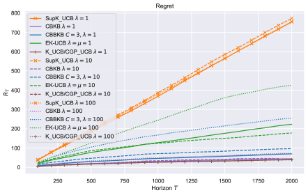
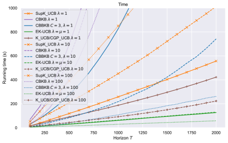
Figure 3: ’Bump’ setting: Regret and running times of EK-UCB, CBBKB and CBKB, with $T=2000$ and $\lambda=\mu$ (see Corollary 3.1 and 4.1) with varying $\lambda$ and $C=3$ for CBBKB. EK-UCB matches the best regret-time compromise.

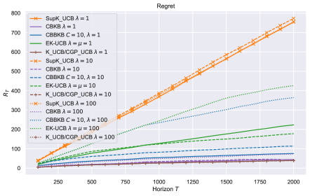
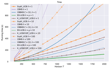
Figure 4: ’Bump’ setting: Regret and running times of EK-UCB, CBBKB and CBKB, with $T=2000$ and $\lambda=\mu$ with varying $\lambda$ and $C=10$ for CBBKB. EK-UCB matches the best regret-time compromise.

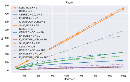
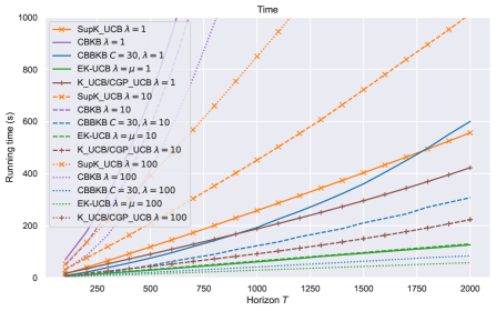
Figure 5: ’Bump’ setting: Regret and running times of EK-UCB, CBBKB and CBKB, with $T=2000$ and $\lambda=\mu$ with varying $\lambda$ and $C=30$ for CBBKB. EK-UCB matches the best regret-time compromise

More dictionary updates lead to better regret but a higher computational complexity

We note that the CBKB baseline achieves satisfactory regret but with a drastically higher computational time. This is due to the fact that it resamples the dictionary at each step and therefore resamples a dictionary at the price of a higher time complexity. As for CBBKB, throughout the Figures 3, 4, 5, we can see that the accumulation threshold $C$ that controls the anchor point update frequency determines the regret-time compromise. The lower $C$, the better is the regret but the higher is the computational time. We can see through the figures that for all values of $C$, our EK-UCB method achieves similar or better (especially when $C=30$) regret than CBBKB while always being both faster than CBBKB but more importantly faster than K-UCB. Overall, EK-UCB proposes the most satisfactory regret-time compromise. Moreover, we see that the SupK-UCB method also performs poorly even with different parameters $\lambda$ and that the optimized K-UCB method also performs better than efficient strategies when the computational overheads of dictionary buildings overtake the efficient kernel approximations.

The regularization parameter controls the regret-time comprise in EK-UCB

In our method, we can see that the higher $\lambda$ (with $\lambda=\mu$) the faster the algorithm is but the worse is its regret. As discussed in Corollary 3.1 and 4.1, we use the heuristic to take $\lambda\approx\sqrt{T}$ and set $\mu=\lambda$ afterwards to enjoy the optimal guarantees of our algorithm.

F.2.2 Additional synthetic settings

In this section we introduce additional settings that we call the ’Chessboard’ setting as well as the ’Step Diagonal’ setting. The two settings lead to similar numerical conclusions as the previous one. We provide more discussions here.

Chessboard and Step Diagonal synthetic setups.

The ’Chessboard’ synthetic setup is a contextual environment with a piecewise reward function over the joint context-action space $\mathcal{X}\times\mathcal{A}=[0,1]\times[0,1]$. More precisely, the joint 2D space is cut into a grid where the values are either 1, 0.5 or 0 according to the part of the grid. Results are shown in Figures 7, 8, 9. The ’Step diagonal’ synthetic setup is a contextual environment with a diagonal reward function over the joint context-action space $\mathcal{X}\times\mathcal{A}=[0,1]\times[0,1]$. More precisely, the joint 2D space has values of 0 everywhere except along two bands along the diagonal where the action and context values are identical with values 0.5 and 1 respectively on the sub diagonal and the above diagonal. Results are shown in Figures 10, 11, 12. See the code for more details and an illustration of the settings in Fig 6.

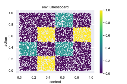
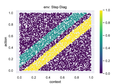
Figure 6: Chessboard (left) and Step Diagonal (right) synthetic setups.

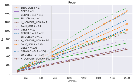
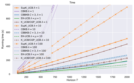
Figure 7: ’Chessboard’ setting: Regret and running times of EK-UCB, CBBKB and CBKB, with $T=2000$ and $\lambda=\mu$ with varying $\lambda$ and $C=3$ for CBBKB.

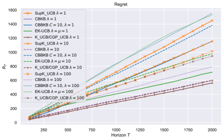
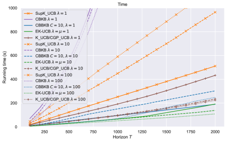
Figure 8: ’Chessboard’ setting: Regret and running times of EK-UCB, CBBKB and CBKB, with $T=2000$ and $\lambda=\mu$ with varying $\lambda$ and $C=10$ for CBBKB.

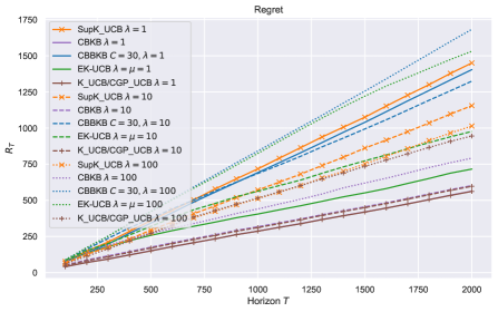
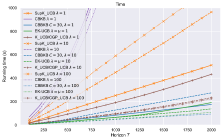
Figure 9: ’Chessboard’ setting: Regret and running times of EK-UCB, CBBKB and CBKB, with $T=2000$ and $\lambda=\mu$ with varying $\lambda$ and $C=30$ for CBBKB.

Regret-time compromise for CBBKB and EK-UCB.

The two settings show what both algorithms CBBKB and EK-UCB achieve as a regret-time compromise. In cases where $C$ is lower (note that CBKB corresponds to CBBKB with $C=1$) the regret often decreases at the price of higher computational time complexity. Similarly, we can notice that our method has better regrets when $\lambda$ is low, but with higher computational times, while still providing a benefit over to the K-UCB method, unlike CBBKB. We therefore note again that in practice, dictionary building computational overheads may influence the global computational complexity. Overall, our method with its incremental dictionary building strategy achieves the best satisfactory time-regret compromises in the Chessboard and Step Diagonal settings compared to both K-UCB and the efficient algorithms CBKB and CBBKB.

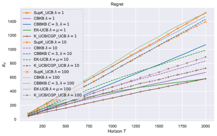
Figure 10: ’Step Diagonal’ setting: Regret and running times of EK-UCB, CBBKB and CBKB, with $T=2000$ and $\lambda=\mu$ with varying $\lambda$ and $C=3$ for CBBKB.

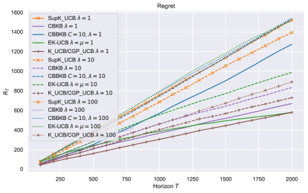
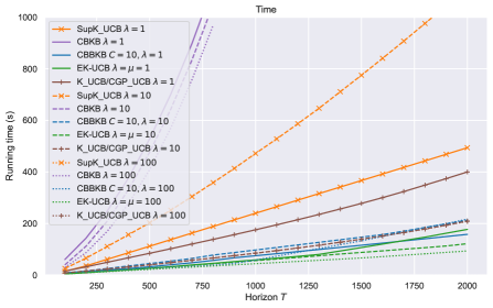
Figure 11: ’Step Diagonal’ setting: Regret and running times of EK-UCB, CBBKB and CBKB, with $T=2000$ and $\lambda=\mu$ with varying $\lambda$ and $C=10$ for CBBKB.

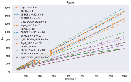
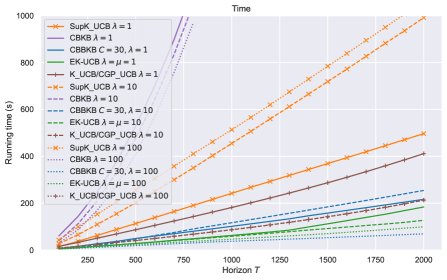
Figure 12: ’Step Diagonal’ setting: Regret and running times of EK-UCB, CBBKB and CBKB, with $T=2000$ and $\lambda=\mu$ with varying $\lambda$ and $C=30$ for CBBKB.

References

- Abbasi-yadkori et al. (2011) Y. Abbasi-yadkori, D. Pál, and C. Szepesvári. Improved algorithms for linear stochastic bandits. In Adv. Neural Information Processing Systems (NIPS), 2011.
- Calandriello et al. (2017a) D. Calandriello, A. Lazaric, and M. Valko. Efficient second-order online kernel learning with adaptive embedding. In Adv. Neural Information Processing Systems (NIPS), 2017a.
- Calandriello et al. (2017b) D. Calandriello, A. Lazaric, and M. Valko. Second-order kernel online convex optimization with adaptive sketching. In International Conference on Machine Learning (ICML), 2017b.
- Calandriello et al. (2019) D. Calandriello, L. Carratino, A. Lazaric, M. Valko, and L. Rosasco. Gaussian process optimization with adaptive sketching: Scalable and no regret. In Conference on Learning Theory (COLT), 2019.
- Calandriello et al. (2020) D. Calandriello, L. Carratino, A. Lazaric, M. Valko, and L. Rosasco. Near-linear time Gaussian process optimization with adaptive batching and resparsification. In International Conference on Machine Learning (ICML), 2020.
- Camilleri et al. (2021) R. Camilleri, J. Katz-Samuels, and K. Jamieson. High-dimensional experimental design and kernel bandits. In International Conference on Machine Learning (ICML), 2021.
- Chowdhury and Gopalan (2017) S. R. Chowdhury and A. Gopalan. On kernelized multi-armed bandits. In International Conference on Machine Learning (ICML), 2017.
- Derezinski et al. (2020) M. Derezinski, F. Liang, and M. Mahoney. Bayesian experimental design using regularized determinantal point processes. In International Conference on Artificial Intelligence and Statistics (AISTATS), 2020.
- Hastie et al. (2001) T. Hastie, R. Tibshirani, and J. Friedman. The Elements of Statistical Learning. Springer Series in Statistics. 2001.
- Jézéquel et al. (2019) R. Jézéquel, P. Gaillard, and A. Rudi. Efficient online learning with kernels for adversarial large scale problems. In Adv. in Neural Information Processing Systems (NeurIPS). 2019.
- Krause and Ong (2011) A. Krause and C. S. Ong. Contextual gaussian process bandit optimization. In Adv. Neural Information Processing Systems (NIPS), 2011.
- Kuzborskij et al. (2019) I. Kuzborskij, L. Cella, and N. Cesa-Bianchi. Efficient linear bandits through matrix sketching. In International Conference on Artificial Intelligence and Statistics (AISTATS), 2019.
- Lattimore and Szepesvári (2020) T. Lattimore and C. Szepesvári. Bandit Algorithms. Cambridge University Press, 2020.
- Li et al. (2010) L. Li, W. Chu, J. Langford, and R. E. Schapire. A contextual-bandit approach to personalized news article recommendation. In International Conference on World Wide Web (WWW), 2010.
- Mahoney and Drineas (2009) M. W. Mahoney and P. Drineas. Cur matrix decompositions for improved data analysis. Proceedings of the National Academy of Sciences (PNAS), 106(3):697–702, 2009.
- Mutnỳ and Krause (2019) M. Mutnỳ and A. Krause. Efficient high dimensional bayesian optimization with additivity and quadrature fourier features. In Adv. in Neural Information Processing Systems (NeurIPS), 2019.
- Rudi et al. (2015) A. Rudi, R. Camoriano, and L. Rosasco. Less is more: Nyström computational regularization. In Adv. in Neural Information Processing Systems (NIPS), 2015.
- Scarlett et al. (2017) J. Scarlett, I. Bogunovic, and V. Cevher. Lower bounds on regret for noisy gaussian process bandit optimization. In Conference on Learning Theory (COLT), 2017.
- Srinivas et al. (2010) N. Srinivas, A. Krause, S. M. Kakade, and M. W. Seeger. Gaussian process optimization in the bandit setting: No regret and experimental design. In International Conference on Machine Learning (ICML), 2010.
- Tirinzoni et al. (2020) A. Tirinzoni, M. Pirotta, M. Restelli, and A. Lazaric. An asymptotically optimal primal-dual incremental algorithm for contextual linear bandits. In NeurIPS, 2020.
- Valko et al. (2013) M. Valko, N. Korda, R. Munos, I. Flaounas, and N. Cristianini. Finite-time analysis of kernelised contextual bandits. In Conference on Uncertainty in Artificial Intelligence (UAI), 2013.
- Williams and Seeger (2001) C. K. Williams and M. Seeger. Using the nyström method to speed up kernel machines. In Adv. Neural Information Processing Systems (NIPS), 2001.