High-dimensional Inference and FDR Control for Simulated Markov Random Fields
Abstract
Identifying important features linked to a response variable is a fundamental task in various scientific domains. This article explores statistical inference for simulated Markov random fields in high-dimensional settings. We introduce a methodology based on Markov Chain Monte Carlo Maximum Likelihood Estimation (MCMC-MLE) with Elastic-net regularization. Under mild conditions on the MCMC method, our penalized MCMC-MLE method achieves -consistency. We propose a decorrelated score test, establishing both its asymptotic normality and that of a one-step estimator, along with the associated confidence interval. Furthermore, we construct two false discovery rate control procedures via the asymptotic behaviors for both p-values and e-values. Comprehensive numerical simulations confirm the theoretical validity of the proposed methods.
1 Introduction
1.1 Backgrounds and Related Work
The probabilistic graphical model is a framework comprising various probability distributions that decompose based on the architecture of an associated graph [66]. This model adeptly encapsulates the intricate interdependencies among random variables, enabling the construction of extensive multivariate statistical models. These models have found extensive applications across diverse research domains. Notably, they are utilized in hierarchical Bayesian models [35], and in the analysis of contingency tables [26, 69], a key aspect of categorical data analysis [1, 29]. Within these graphical models, undirected graphical models stand out, characterized by a probability distribution that factorizes based on functions defined over the graph’s cliques. These undirected graphical models typically play a critical role in constraint satisfaction problems [20, 17], and have significant applications in language and speech processing [11, 14]. Their utility extends to image processing [21, 30, 36] and more broadly in the realm of spatial statistics [9], demonstrating their versatility and importance in contemporary research. These models are widely employed in diverse fields such as statistical physics [41], natural language processing [46], image analysis [70], and spatial statistics [53].
Our focus narrows specifically to undirected graphical models conceptualized as exponential families. This broad category of probability distributions has been extensively examined in statistical literature [5, 27]. The characteristics of exponential families forge insightful links between inference methodologies and convex analysis [13, 39]. Notably, many renowned models are perceived as exponential families within undirected graphical models, including the Ising model [41, 6], Gaussian random fields [58], and latent Dirichlet allocation [11]. These models are all special instances of Markov Random Fields (MRFs) framed within exponential families [56]. Consequently, our paper will concentrate on this particular aspect of MRFs.
In the realm of graphical models, two crucial aspects are structure learning and parameter estimation [66, 42, 49, 18]. The significance of Markov Random Fields (MRFs) with exponential families necessitates effective solutions tailored to this specific framework. A primary challenge in learning the structure of such models is the computationally daunting normalizing constant. In a scenario where a graphical model comprises vertices, with each variable at a vertex assuming values from a discrete state space of distinct elements, the normalizing constant escalates to a sum of terms, rendering computation impractical. To address this challenge, numerous methods have been proposed. A prominent approach is the pseudo-likelihood method [9], which substitutes the likelihood involving the normalizing constant with the product of conditional probabilities that do not include this constant. However, its effectiveness is contingent on the pseudo-likelihood being a close approximation to the actual likelihood, which typically occurs in graphs with simpler structures. Another notable strategy to tackle the intractable normalizing constant is the Markov Chain Monte Carlo (MCMC) method [34, 54]. Here, the normalizing constant is approximated through a path integral over a Markov chain. A significant advantage of the MCMC method is that its computational cost does not depend on the complexity of the graph being estimated. This implies that sufficiently large sample sizes can effectively approximate the normalizing constant, offering a viable solution for handling more complex graphical structures.
In the evolving landscape of graphical models, a notable trend is their increasing dimensionality, often resulting in high-dimensional settings [48, 37, 45]. In such scenarios, where the number of parameters () exceeds the number of independent samples (), the maximum likelihood estimation becomes problematic. To address this, the Lasso method, a penalty, is commonly applied [60], effectively constraining parameters to prevent overfitting. While Lasso can zero out certain parameters, ridge regression ensures that no parameter is entirely excluded. The Elastic-net method, a combination of Lasso (-)penalty and ridge (-)penalty [74], will be used in our study. This approach, often outperforming Lasso in practice, can select multiple correlated variables simultaneously, demonstrating a group effect and handling multicollinearity effectively. Another challenge in a high-dimensional graphical model is discerning the most influential factors, crucial in fields like genomics for identifying genes related to specific diseases. The false discovery rate (FDR), as proposed by [7], is preferred over the family-wise error rate (FWER) in these scenarios due to its suitability for large-scale hypothesis testing. The Benjamini-Hochberg (BH) procedure [7] is commonly used for controlling the FDR, especially effective with asymptotically normal estimators in high dimensions. Additionally, e-values [65] have emerged as a novel and mathematically convenient tool for multiple testing, gaining prominence in statistical analysis [64, 22].
In high-dimensional graphical models, a significant hurdle is the estimation of the intractable normalizing constant from the Markov Chain Monte Carlo (MCMC) component. In low-dimensional cases, the normalizing constant is often linked to MCMC-MLE, the minimization of the MCMC approximation of the likelihood, as discussed in various studies [32, 33, 3]. However, the high-dimensional scenario introduces the complexity of numerous nuisance parameters, rendering traditional partial-likelihood-based inferences impractical. To address this, some researchers have explored penalized MCMC approximations of the likelihood. For example, [49] applied an penalty to the MCMC approximation for the Ising model, while [31] implemented an penalty for discrete MRFs. Additionally, [12] discussed the potential of this approach in Bayesian logic regression using arbitrary priors from MCMC-MLE. Despite these advancements, there remains a big gap in the literature regarding the analysis of general MRFs within the exponential family for high-dimensional settings.
1.2 Our Contributions
In our study, we bridge a significant gap by integrating - and -penalties in the MCMC-MLE for general MRFs within the exponential family. Our contributions are three-fold. First, we derive an oracle inequality for the MCMC-MLE under Elastic-net penalty, establishing the -consistency of the estimator under conditions such as the compatibility condition [61, 15]; see Appendix A.
To address the issue of high-dimensional nuisance parameters, we construct a decorrelated score function by projecting the score function of the parameter onto the space spanned by the nuisance parameters. This approach yields a corresponding decorrelated score test statistic [51, 57, 19] and facilitates the proposal of an asymptotically unbiased one-step estimator. We establish asymptotic normality and confidence intervals in our work, aligning with high-dimensional inferential statistics. with a stronger assumption , where denotes the sample size, and signifies the dimension of the model parameter. Achieving the desired asymptotic normality with the introduction of the Monte Carlo method and simulated samples necessitates the acceleration of its convergence. This requires the assumption , marking a theoretical breakthrough and a notable departure from current literature.
1.3 Outline and Notations
The paper is outlined as follows. The paper is outlined as follows. Section 2 provides background: it gives an overview of graphical models, the MCMC-MLE method, Elastic-net penalized estimation for high-dimensional data, and concentration inequalities for Markov chains. Section 3 constructs the decorrelated score function and corresponding test statistic, proving their asymptotic normality. This section also introduces an asymptotically unbiased one-step estimator used to formulate a confidence interval for a single parameter of interest. Section 4 presents two distinct procedures for controlling the FDR, utilizing p-values and e-values. Finally, Section 5 conducts simulations to validate the theoretical aspects discussed.
Throughout the paper, we define the following notations. Let be a series of random variables and a series of constants. The notation is used to denote that converges to zero in probability as tends to infinity. Conversely, indicates that the set of random variables is stochastically bounded. For two series of constants and , the notation implies the existence of a constant such that for all . Analogously, indicates the lower bound. Let denote weak convergence. The notation is used when both and hold true.
2 Preliminaries
2.1 Graphical Models within Exponential Families
Define graph model , where is a set of vertices and is a set of edges. For each vertex , assign a random variable To establish a probability distribution associated with the graph. In our study, we focus on the finite discrete state space . We denote the Cartesian product of the state spaces —where the random vector takes values—by . The notation represents a specific element in , and signifies a specific value within the space . For any subset of the vertex set , we define as the sub-vector of the random vector and as a specific element of the random sub-vector.
The undirected graphical models are factorized according to a function defined over the graph’s cliques. A clique is identified as a fully connected subset of the vertex set, satisfying for every . For each clique , we introduce a compatibility function . Let represent a set of the graph’s cliques. The undirected graphical model also referred to as the Markov random field (MRF, [44]), is expressed as
with is the constant chosen to normalize the distribution. Concentrating on the canonical exponential family. the probability mass function for is given by
and is the unknown parameters of interest. Denote . Let and be the expectation and covariance of the random vector , respectively. Specifically, by taking where , the model evolves into the Ising model in [49]. Further, constraining for any transforms the model into the discrete MRFs, also discussed in [31]. Consequently, our model is considerably more general than those in the existing literature.
2.2 Penalized Markov Chain Monte Carlo Likelihood
Suppose are independent and identically distributed from distribution , where is the true parameter. We construct the negative log-likelihood function as follows:
| (1) |
We then employ the MCMC method for approximation of the normalized constant . Consider as a Markov chain with its stationary distribution on the product space being . By the ergodic property of the Markov chain, can be approximated through a path integral
| (2) |
Combining (1) and (2), the MCMC log-likelihood function is
Denote and Then the gradient and the Hessian can be re-expressed as
| (3) |
| (4) |
It is clear that is convex. Denote as the covariance matrix of the function under the true value .
In high-dimensional cases where the number of parameters significantly exceeds the number of samples (), the minimum of is not unique, resulting in an ill-posed minimizer of MCMC log-likelihood. To address this issue, we consider deploying a penalty to the likelihood function in this article. We employ the Elastic-net penalty, which combines the benefits of both the Lasso method and ridge regression. The Elastic-net-penalized MCMC-MLE we propose is formulated as
| (5) |
where are two tuning parameters. The terms and represent the -norm and -norm of the vector , respectively.
3 Decorrelated Score Test and Confidence Interval
In high-dimensional inference, testing a specific element within the true vector presents some challenges. Unlike low-dimensional scenarios, the presence of a high-dimensional nuisance parameter set complicates the development of valid inferential methods. Traditional approaches like partial-likelihood-based inference [51, 28, 57], become impractical in this context due to the intractability of the limiting distribution and the complexity introduced by numerous nuisance parameters. Motivated from [28], we propose a decorrelated score test to address the hypothesis testing of versus . This approach is analogous to the traditional score test but modified to suit high-dimensional contexts. In such settings, a direct extension of the profile partial score test becomes infeasible due to the intractable limiting distribution caused by the large number of nuisance parameters. We address this challenge by adopting a decorrelated method inspired by a projection technique, which helps to mitigate the influence of these nuisance parameters.
Without loss of generality, consider as , with being the first scalar component. The gradients and Hessian are partitioned as and . Similarly, we denote the blocks of as . To test the hypothesis , we first estimate the nuisance parameters by using the Elastic-net-penalized MCMC-MLE defined in (5). Then, we approximate using the partial score function in terms of expectation:
where is the projection of onto the linear space spanned by elements. In high-dimension case, direct computation of from sample data is problematic, so we estimate using a lasso-type estimator :
where is another tuning parameter. Building upon this, we propose a decorrelated score function:
| (6) |
Intuitively, this decorrelated score function removes the effects of the high-dimensional nuisance parameters [51]. Then to establish the limiting distribution of under the null hypothesis , the following assumptions regarding the properties of the covariance matrix and the weight vector are required.
Assumption 3.1.
The eigenvalues of the covariance matrix are lower and upper bounded: for some .
Assumption 3.2.
The -norm of is bounded: for some .
Define the -norm as for any vector , and let and . The following lemmas establish the asymptotic normality of and the consistency of the estimator .
Lemma 3.2 implies that the sparsity parameters of are essential for the asymptotic normality of and the consistency of . Additionally, the condition is required to ensure the consistency of . We now present the main result of the proposed method, which demonstrates the asymptotic normality of the decorrelated score function under the null.
Theorem 3.1.
Theorem 3.1 indicates that to achieve the asymptotic normality of the decorrelated score function, we require the condition , which is a stronger assumption than , necessary for the -consistency of . This stronger assumption aligns with existing literature for proportional hazards models [28] and broader statistical frameworks [51]. Note that the asymptotic variance is unknown. Thus, we estimate the variance of the limiting normal distribution with .
And thus, we define the decorrelated score test statistic as
by Theorem 3.1 and Lemma 3.3, we know that the asymptotic distribution of is a standard normal distribution under . Next, we focus on developing a confidence interval for the true parameter . This approach addresses the limitation noted earlier, where the decorrelated score function did not directly yield a confidence interval for .
The key idea to derive a confidence interval for is based on the decorrelated score function . Drawing from Theorem 3.1 and leveraging the properties of Z-estimators as outlined in [63], we find that the solution to the equation closely approximates . However, directly solving the estimation equation is computationally challenging. To circumvent this, we employ a method that linearizes around the penalized estimator , leading to the introduction of the following one-step estimator :
| (7) |
where is derived from the Elastic-net-penalized MCMC-MLE in (5), and is defined as the decorrelated score test in (6). Notably, the formulation of parallels the application of a one-step iteration at the initial point , akin to Newton’s method, for solving .
A key advantage of the one-step estimator in high-dimensional settings is its asymptotic normality, a property not shared by traditional penalty estimators such as ; this is detailed in the theorem below.
Theorem 3.2.
4 FDR Control
In this section, we develop two effective false discovery rate (FDR) control procedures using p-values and e-values. Specifically, we define a specific “metric" value to assess the confidence level associated with each component of via data splitting for the p-value based approach; and further introduce the e-value based approach to facilitate more streamlined computations.
Formally speaking, FDR control is for the multiple hypothesis testing when addressing a series of hypotheses, such as for each in . Here, signifies the pre-established value against which the true value is tested [7, 8, 59]. Consider as the set encompassing unknown true null hypotheses. The FDR control process, based on certain statistical measures, decides on the acceptance or rejection of each hypothesis . The subset , identified as discoveries in the literature, represents those hypotheses rejected. The intersection , known as false discoveries, includes the true null hypotheses erroneously rejected. The false discovery proportion (FDP), defined as , is a critical metric indicating the efficacy of the FDR control procedure. Notably, is a random variable, but the emphasis is on its expected value under the data’s generating distribution, referred to as FDR represented as
Crafting an effective FDR control strategy is a fundamental task in multiple hypothesis testing to control the type-I errors [59, 64, 67].
4.1 FDR control via p-values
False discovery rate is a profound p-value based criterion for controlling uncertainty and avoiding spurious discoveries in multiple testing [7]. Nevertheless, the challenge with classical p-values arises from their inter-correlation, which prevents straightforward summation for statistical analysis. To address the dependence, data splitting is effective in constructing data-driven mirror statistics [23, 25]
where is a function that is non-negative, symmetric, and exhibits monotonic increase for both and and is the sign function. The term represents the normalized estimates for in the -th partition of the entire dataset. Specifically, we employ
where denotes the one-step estimator of in (7) and . Thus, we first split the data into two disjoint parts, and then run Algorithm 1 analogous to that in [23] to asymptotically control the FDR.
We necessitate an additional assumption to theoretically substantiate our method for controlling the FDR.
Assumption 4.1.
The indices are exchangeable. Specifically, for the population version , we have that and .
Assumption 4.1 is commonly encountered in the literature on multiple hypothesis testing, underpinning the concept of ‘knockoff filtering’ [4, 55, 40, 18]. This assumption is satisfied by a broad spectrum of models within the exponential family of MRFs, including Ising model and the Gaussian graphical model.
Theorem 4.1.
Theorem 4.1 validates that single data split (Algorithm 1) yields effective FDR at the target level. However, potential loss of power or instability [23] are involved due to the split randomness. To mitigate these issues, we consider multiple data splits, akin to the approach described in [23]. Define
where denotes the set of selected features in the -th data split as determined by Algorithm 1. Set if . The term represents the inclusion rate, reflecting the extent to which information about is captured within the selected set .
4.2 FDR control via e-values
Controlling FDR typically aims to restrict the expected proportion of Type I errors, which involve the incorrect rejection of a true null hypothesis. The p-value based approaches are typically adept at closely controlling the FDR at a pre-specified level, implying a concurrent tendency to manage Type II errors – the probability of erroneously retaining a false null hypothesis [23, 24] However, in some scenarios, the focus on Type II error is less critical, allowing for the possibility of controlling the FDR at levels significantly below the designated threshold. This approach may be overly stringent, but if such strictness is not a concern, it can be an effective strategy. In these instances, the e-BH procedure proves beneficial [64, 65, 68]. The e-values are characterized by their additivity, independent of the correlation among covariates. This unique attribute simplifies and streamlines the FDR control process using e-values, compared to approaches based on p-values. In this section, we will design the e-BH procedure in [64, 65, 68], and then analyze the asymptotic properties of the proposed methods.
The key to a valid e-value procedure is the establishment of an e-variable such that under the null hypothesis [65]. When the hypothesis is true, by (8) we observe that , leading to . Based on this, we propose the following Algorithm 3.
| (10) |
For the purpose of avoiding overly complex structures in the index set, we introduce the following assumption.
Assumption 4.2.
For any ,
Assumption 4.2 is pivotal in ensuring average convergence on sets with diverging numbers of elements. However, this assumption can be relaxed with additional constraints on the data, as discussed in Section 4 of [16]. Under this assumption, the following theorem addressees the control of FDR in an asymptotic framework.
5 Simulation Studies
In this section, we conduct extensive numerical studies to assess the finite sample performance of the proposed procedure. We generate i.i.d. from with . The following scenarios for are investigated:
-
•
.
-
•
.
-
•
.
Utilizing the Metropolis sampling method [38], we generate samples , treating as an i.i.d. sample. In each simulation, cross-validation is employed to select the tuning parameters . The elements of the true parameter are generated from , where and are independently uniformly distributed over . We set the simulated sample size as . All the simulation results are based on replications.
| 50 | 100 | 150 | 200 | 250 | 300 | 350 | 400 | 450 | 500 | |
| 100 | 0.0583 | 0.1232 | 0.2042 | 0.5108 | 1.8834 | 1.5548 | 1.5819 | 2.0679 | 2.9404 | 3.7422 |
| 200 | 0.0422 | 0.0751 | 0.0903 | 0.1596 | 0.2024 | 0.2187 | 0.4313 | 0.5091 | 0.5176 | 1.1599 |
| 300 | 0.0354 | 0.0541 | 0.0909 | 0.1052 | 0.1183 | 0.1741 | 0.2058 | 0.2232 | 0.2828 | 0.3410 |
| 400 | 0.0326 | 0.0614 | 0.0965 | 0.1044 | 0.0863 | 0.1089 | 0.1622 | 0.1689 | 0.1952 | 0.2074 |
| 500 | 0.0762 | 0.0853 | 0.0550 | 0.0783 | 0.0930 | 0.1220 | 0.1221 | 0.1227 | 0.1615 | 0.1903 |
| 600 | 0.0219 | 0.0565 | 0.0453 | 0.0696 | 0.0695 | 0.0821 | 0.1344 | 0.1116 | 0.1513 | 0.1390 |
| 700 | 0.0281 | 0.0377 | 0.0476 | 0.0612 | 0.0714 | 0.0920 | 0.0914 | 0.1051 | 0.1102 | 0.1218 |
| 800 | 0.0230 | 0.0550 | 0.0373 | 0.1000 | 0.0755 | 0.0710 | 0.1041 | 0.0957 | 0.1244 | 0.1294 |
| 900 | 0.0218 | 0.0351 | 0.0667 | 0.0617 | 0.0651 | 0.0614 | 0.0788 | 0.0911 | 0.0888 | 0.1185 |
| 1000 | 0.0521 | 0.0452 | 0.0854 | 0.0495 | 0.0620 | 0.0737 | 0.0794 | 0.0795 | 0.0998 | 0.1097 |
| 50 | 100 | 150 | 200 | 250 | 300 | 350 | 400 | 450 | 500 | |
| 100 | 0.2420 | 0.9483 | 0.0920 | 3.7035 | 5.7790 | 0.9768 | 11.1498 | 14.4463 | 18.1982 | 19.6261 |
| 200 | 0.1179 | 0.4703 | 0.1048 | 0.1615 | 2.8785 | 0.2173 | 5.5507 | 7.1994 | 9.3011 | 11.4753 |
| 300 | 0.0790 | 0.3118 | 0.0252 | 1.2319 | 0.0555 | 0.0748 | 3.7021 | 4.7937 | 6.1796 | 8.6076 |
| 400 | 0.0596 | 0.2335 | 0.0174 | 0.9251 | 1.4300 | 0.2248 | 2.7787 | 3.6098 | 4.6258 | 5.7292 |
| 500 | 0.0475 | 0.1853 | 0.4183 | 0.0309 | 1.1425 | 0.1636 | 0.1216 | 2.8813 | 3.6366 | 4.5797 |
| 600 | 0.0393 | 0.1545 | 0.0189 | 0.0264 | 0.9494 | 0.1365 | 0.1844 | 2.3881 | 0.2575 | 0.4251 |
| 700 | 0.0332 | 0.1329 | 0.0110 | 0.0621 | 0.8180 | 0.0577 | 0.1580 | 2.0542 | 2.6547 | 0.3268 |
| 800 | 0.0297 | 0.1164 | 0.2591 | 0.0239 | 0.7172 | 0.0361 | 0.1384 | 0.1570 | 0.1404 | 0.2866 |
| 900 | 0.0261 | 0.1033 | 0.0066 | 0.4086 | 0.0246 | 0.0352 | 0.1229 | 0.1583 | 0.1321 | 0.2545 |
| 1000 | 0.0236 | 0.0024 | 0.0208 | 0.0120 | 0.0573 | 0.0818 | 0.1105 | 0.1441 | 0.1205 | 0.1126 |
| 50 | 100 | 150 | 200 | 250 | 300 | 350 | 400 | 450 | 500 | |
| 100 | 0.0744 | 0.0802 | 0.3834 | 0.1714 | 0.6114 | 0.8035 | 0.5839 | 0.4769 | 2.0614 | 6.2039 |
| 200 | 0.0724 | 0.1124 | 0.0550 | 0.1127 | 0.3119 | 1.8504 | 0.2266 | 0.2357 | 0.6231 | 0.8614 |
| 300 | 0.0114 | 0.0465 | 0.0596 | 0.0549 | 0.2676 | 0.1700 | 0.1451 | 0.1181 | 0.4000 | 0.1436 |
| 400 | 0.0095 | 0.0171 | 0.0335 | 0.0427 | 0.5303 | 0.0639 | 0.3037 | 0.1764 | 0.2361 | 1.4182 |
| 500 | 0.0101 | 0.0142 | 0.0235 | 0.0672 | 0.1142 | 0.0819 | 0.8170 | 1.0434 | 0.7713 | 0.1647 |
| 600 | 0.0057 | 0.0135 | 0.0469 | 0.0450 | 0.3342 | 0.2689 | 0.6022 | 0.8204 | 0.6905 | 0.1272 |
| 700 | 0.0060 | 0.0100 | 0.0185 | 0.0258 | 0.0399 | 0.0605 | 0.0472 | 0.8851 | 0.8351 | 0.0566 |
| 800 | 0.0042 | 0.0104 | 0.0210 | 0.0197 | 0.0346 | 0.0485 | 0.0449 | 0.6599 | 0.4567 | 0.0721 |
| 900 | 0.0039 | 0.0086 | 0.0136 | 0.0217 | 0.0261 | 0.0411 | 0.0538 | 0.4903 | 0.0550 | 0.0577 |
| 1000 | 0.0035 | 0.0084 | 0.0308 | 0.0273 | 0.0201 | 0.0267 | 0.0392 | 0.0309 | 0.0695 | 0.0572 |
To assess the estimation performance of the proposed methods, we calculate the -error of the Elastic-net estimator from . Table 1 shows our estimator demonstrating consistency under both low and high-dimensional cases when the tuning parameters and are appropriately selected. This empirically confirms the theoretical consistency guarantee stated in Theorem B.1.
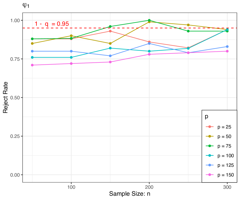
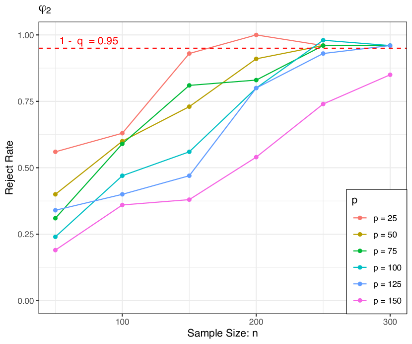
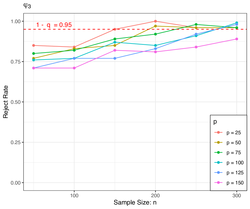
Next, we investigate the one-step estimator with the empirical rejection rate , where represents the number of replications, and and correspond to the values obtained in the -th simulation. For the sake of simplicity, we construct the confidence interval for defined (9). The results of this analysis are depicted in Figure 1.As shown in Figure 1, the one-step estimators exhibit the asymptotic normality stated in Theorem 3.2, without requiring extremely large sample sizes. The empirical rejection rates match the designed confidence level when is around 300. This demonstrates the asymptotic normality holding reasonably well for moderately sized samples.
As for FDR control, we study the traditional false discovery rate control procedures via p-values (Algorithm 1) and the more novel approach utilizing e-values (Algorithm 3) with a nominal level of . Table 2 demonstrates that both the p-value and e-value based procedures effectively maintain the desired level of FDR control. Notably, the e-value based procedure (Algorithm 3) tends to produce a more conservative FDP level. Moreover, the e-value procedure is more computationally efficient than the p-value procedure.
| 50 | 100 | 150 | 200 | 250 | 300 | 350 | 400 | 450 | 500 | |
| 100 | 0.0598, 0.02 | 0.0972, 0 | 0.1234, 0 | 0.1338, 0 | 0.1001, 0 | 0.1387, 0 | 0.1084, 0.02 | 0.1059, 0.06 | 0.0963, 0.04 | 0.0957, 0.102 |
| 200 | 0.0060, 0 | 0.0062, 0 | 0.0325, 0 | 0.0671, 0 | 0.1001, 0 | 0.0706, 0 | 0.1084, 0 | 0.1059, 0 | 0.0963, 0 | 0.0957, 0 |
| 300 | 0.0030, 0 | 0, 0 | 0.0011, 0 | 0.0018, 0 | 0.0148, 0 | 0.0435, 0 | 0.0724, 0 | 0.0928, 0 | 0.0803, 0 | 0.1103, 0 |
| 400 | 0, 0 | 0, 0 | 0, 0 | 0, 0 | 0, 0 | 0.0042, 0 | 0.0116, 0 | 0.0287, 0 | 0.0623, 0 | 0.0672, 0 |
| 500 | 0, 0 | 0, 0 | 0, 0 | 0, 0 | 0, 0 | 0, 0 | 0, 0 | 0, 0 | 0.0066, 0 | 0.0303, 0 |
| 50 | 100 | 150 | 200 | 250 | 300 | 350 | 400 | 450 | 500 | |
| 100 | 0.0162, 0.02 | 0.0584, 0 | 0.0737, 0 | 0.1408, 0 | 0.1289, 0.02 | 0.1105, 0.02 | 0.1171, 0.04 | 0.0647, 0.04 | 0.069, 0.08 | 0.1121, 0.12 |
| 200 | 0, 0 | 0, 0 | 0.0068, 0 | 0.0399, 0 | 0.0723, 0 | 0.1105, 0 | 0.1171, 0 | 0.0073, 0 | 0.0337, 0 | 0.0636, 0 |
| 300 | 0, 0 | 0, 0 | 0, 0 | 0, 0 | 0.0017, 0 | 0.0173, 0 | 0.0348, 0 | 0.0647, 0 | 0.0690, 0 | 0.1121, 0 |
| 400 | 0, 0 | 0, 0 | 0, 0 | 0, 0 | 0, 0 | 0, 0 | 0, 0 | 0.0011, 0 | 0.0254, 0 | 0.0496, 0 |
| 500 | 0, 0 | 0, 0 | 0, 0 | 0, 0 | 0, 0 | 0, 0 | 0, 0 | 0.0005, 0 | 0.0010, 0 | 0.0023, 0 |
| 50 | 100 | 150 | 200 | 250 | 300 | 350 | 400 | 450 | 500 | |
| 100 | 0.0988, 0.08 | 0.1421, 0.02 | 0.1145, 0 | 0.1024, 0.04 | 0.1408, 0.04 | 0.0954, 0.1 | 0.1132, 0.12 | 0.0935, 0.12 | 0.0836, 0.08 | 0.0992, 0.12 |
| 200 | 0.0771, 0.002 | 0.1342, 0 | 0.1145, 0.02 | 0.1024, 0 | 0.1408, 0.02 | 0.0954, 0 | 0.0814, 0.02 | 0.1111, 0.02 | 0.1067, 0.02 | 0.1060, 0.06 |
| 300 | 0.0988, 0 | 0.0408, 0 | 0.0617, 0 | 0.0685, 0 | 0.1138, 0 | 0.1096, 0 | 0.1132, 0 | 0.0935, 0 | 0.0836, 0 | 0.0992, 0 |
| 400 | 0.0697, 0 | 0.0238, 0 | 0.0251, 0 | 0.028, 0 | 0.0346, 0 | 0.0505, 0 | 0.0696, 0 | 0.0885, 0 | 0.0997, 0 | 0.0996, 0 |
| 500 | 0.0405, 0 | 0.0232, 0 | 0.0122, 0 | 0.0076, 0 | 0.0102, 0 | 0.0183, 0 | 0.0223, 0 | 0.0368, 0 | 0.0428, 0 | 0.0556, 0 |
6 Concluding remarks
This paper investigated the estimation and inference of parameters for Markov Random Fields in canonical exponential families. We propose a penalized Markov Chain Monte Carlo Maximum Likelihood method to estimate the intractable normalizing constant in high-dimensional settings. To facilitate statistical inference on the obtained estimates, we subsequently devise a one-step estimator with decorrelated scores and thus present two FDR controlling procedures. Our extensive numerical investigations demonstrate that the proposed methods provide satisfactory performances in estimation and inference. Given our methodology’s reliance on mild assumptions, its broad potential applicability, warrants further research.
Acknowledgments
The research of H. Zhang is supported in part by NSFC Grant No.12101630.
Author contributions statement
H.Z. was the driving force behind the motivation for this study and developed the main ideas. H.W., X.L. and Y.H. were responsible for the writing and rigorous completion of all proofs. H.W. took the lead in implementing the experiments. All authors participated in writing and reviewing the manuscript.
References
- Agresti [2003] Agresti, A. (2003). Categorical Data Analysis, Volume 482. John Wiley & Sons.
- Azriel and Schwartzman [2017] Azriel, D. and A. Schwartzman (2017). The empirical distribution of a large number of correlated normal variables. Journal of the American Statistical Association 110(511), 1217–1228.
- Banerjee et al. [2008] Banerjee, O., L. E. Ghaoui, and A. d’Aspremont (2008). Model Selection through Sparse Maximum Likelihood Estimation for Multivariate Gaussian or Binary Data. The Journal of Machine Learning Research 9(Mar), 485–516.
- Barber and Candès [2015] Barber, R. F. and E. J. Candès (2015). Controlling the false discovery rate via knockoffs. The Annals of Statistics 43(5).
- Barndorff-Nielsen [2014] Barndorff-Nielsen, O. E. (2014). Information and Exponential Families: in Statistical Theory. John Wiley & Sons.
- Baxter [2016] Baxter, R. J. (2016). Exactly Solved Models in Statistical Mechanics. Elsevier.
- Benjamini and Hochberg [1995] Benjamini, Y. and Y. Hochberg (1995). Controlling the false discovery rate: a practical and powerful approach to multiple testing. Journal of the Royal Statistical Society: Series B (Methodological) 57(1), 289–300.
- Benjamini and Yekutieli [2001] Benjamini, Y. and D. Yekutieli (2001). The control of the false discovery rate in multiple testing under dependency. The Annals of Statistics, 1165–1188.
- Besag [1974] Besag, J. (1974). Spatial Interaction and the Statistical Analysis of Lattice Systems. Journal of the Royal Statistical Society: Series B (Methodological) 36(2), 192–225.
- Bickel et al. [2009] Bickel, P. J., Y. Ritov, and A. B. Tsybakov (2009). Simultaneous Analysis of Lasso and Dantzig Selector. The Annals of Statistics 37(4), 1705–1732.
- Blei et al. [2003] Blei, D. M., A. Y. Ng, and M. I. Jordan (2003). Latent Dirichlet Allocation. The Journal of Machine Learning Research 3(Jan), 993–1022.
- [12] Bogdan, M., B. Miasojedow, and J. Wallin. Discussion of” a novel algorithmic approach to bayesian logic regression” by a. hubin, g. storvik and f. frommlet.
- Borwein and Lewis [2010] Borwein, J. and A. S. Lewis (2010). Convex Analysis and Nonlinear Optimization: Theory and Examples. Springer Science & Business Media.
- Brown [1986] Brown, L. D. (1986). Fundamentals of statistical exponential families: with applications in statistical decision theory. Ims.
- Bühlmann [2013] Bühlmann, P. (2013). Statistical significance in high-dimensional linear models. Bernoulli 19(4), 1212–1242.
- Chakrabortty et al. [2018] Chakrabortty, A., P. Nandy, and H. Li (2018). Inference for individual mediation effects and interventional effects in sparse high-dimensional causal graphical models. arXiv preprint arXiv:1809.10652.
- Chandrasekaran et al. [2012] Chandrasekaran, V., N. Srebro, and P. Harsha (2012). Complexity of Inference in Graphical Models. arXiv preprint arXiv:1206.3240.
- Chen et al. [2023] Chen, S., Z. Li, L. Liu, and Y. Wen (2023). The systematic comparison between gaussian mirror and model-x knockoff models. Scientific Reports 13(1), 5478.
- Chernozhukov et al. [2023] Chernozhukov, V., D. Chetverikov, K. Kato, and Y. Koike (2023). High-dimensional data bootstrap. Annual Review of Statistics and Its Application 10, 427–449.
- Cook [1971] Cook, S. A. (1971). The Complexity of Theorem-Proving Procedures. In Proceedings of the third annual ACM symposium on Theory of computing, pp. 151–158.
- Cross and Jain [1983] Cross, G. R. and A. K. Jain (1983). Markov Random Field Texture Models. IEEE Transactions on Pattern Analysis and Machine Intelligence PAMI-5(1), 25–39.
- Cui et al. [2021] Cui, C., J. Jia, Y. Xiao, and H. Zhang (2021). Directional fdr control for sub-gaussian sparse glms. arXiv preprint arXiv:2105.00393.
- Dai et al. [2022] Dai, C., B. Lin, X. Xing, and J. S. Liu (2022). False discovery rate control via data splitting. Journal of the American Statistical Association, 1–18.
- Dai et al. [2023] Dai, C., B. Lin, X. Xing, and J. S. Liu (2023). A scale-free approach for false discovery rate control in generalized linear models. Journal of the American Statistical Association, 1–15.
- Du et al. [2023] Du, L., X. Guo, W. Sun, and C. Zou (2023). False discovery rate control under general dependence by symmetrized data aggregation. Journal of the American Statistical Association 118(541), 607–621.
- Edwards and Kreiner [1983] Edwards, D. and S. Kreiner (1983). The Analysis of Contingency Tables by Graphical Models. Biometrika 70(3), 553–565.
- Efron [1978] Efron, B. (1978). The Geometry of Exponential Families. The Annals of Statistics 6(2), 362–376.
- Fang et al. [2017] Fang, E. X., Y. Ning, and H. Liu (2017). Testing and Confidence Intervals for High Dimensional Proportional Hazards Models. Journal of the Royal Statistical Society: Series B (Methodological) 79(5), 1415–1437.
- Fienberg [2000] Fienberg, S. E. (2000). Contingency Tables and Log-Linear Models: Basic Results and New Developments. Journal of the American Statistical Association 95(450), 643–647.
- Geman and Geman [1984] Geman, S. and D. Geman (1984). Stochastic Relaxation, Gibbs Distributions, and the Bayesian Restoration of Images. IEEE Transactions on Pattern Analysis and Machine Intelligence PAMI-6(6), 721–741.
- Geng et al. [2018] Geng, S., Z. Kuang, J. Liu, S. Wright, and D. Page (2018). Stochastic learning for sparse discrete markov random fields with controlled gradient approximation error. In Uncertainty in artificial intelligence: proceedings of the… conference. Conference on Uncertainty in Artificial Intelligence, Volume 2018, pp. 156. NIH Public Access.
- Geyer [1992] Geyer, C. J. (1992). Markov Chain Monte Carlo Maximum Likelihood. Technical report, Minnesota University, Minneapolis, School Of Statistics.
- Geyer [1994] Geyer, C. J. (1994). On the Convergence of Monte Carlo Maximum Likelihood Calculations. Journal of the Royal Statistical Society: Series B (Methodological) 56(1), 261–274.
- Gilks [2005] Gilks, W. R. (2005). Markov Chain Monte Carlo. Encyclopedia of Biostatistics 4.
- Gyftodimos and Flach [2002] Gyftodimos, E. and P. A. Flach (2002). Hierarchical Bayesian Networks: A Probabilistic Reasoning Model for Structured Domains. In Proceedings of the ICML-2002 Workshop on Development of Representations, pp. 23–30. Citeseer.
- Hassner and Sklansky [1981] Hassner, M. and J. Sklansky (1981). The Use of Markov Random Fields as Models of Texture. In Image Modeling, pp. 185–198. Elsevier.
- Hastie et al. [2015] Hastie, T., R. Tibshirani, and M. Wainwright (2015). Statistical learning with sparsity: the lasso and generalizations. CRC press.
- Hastings [1970] Hastings, W. (1970). Monte carlo sampling methods using markov chains and their applications. Biometrika, 97–109.
- Hiriart-Urruty and Lemaréchal [2013] Hiriart-Urruty, J.-B. and C. Lemaréchal (2013). Convex Analysis and Minimization Algorithms I: Fundamentals, Volume 305. Springer science & business media.
- Huang and Janson [2020] Huang, D. and L. Janson (2020). Relaxing the assumptions of knockoffs by conditioning. The Annals of Statistics 48(5), 3021–3042.
- Ising [1925] Ising, E. (1925). Beitrag zur theorie des ferromagnetismus. Zeitschrift für Physik 31(1), 253–258.
- Jalali et al. [2011] Jalali, A., C. C. Johnson, and P. K. Ravikumar (2011). On Learning Discrete Graphical Models using Greedy Methods. In Advances in Neural Information Processing Systems, pp. 1935–1943.
- Jiang et al. [2018] Jiang, B., Q. Sun, and J. Fan (2018). Bernstein’s inequality for general markov chains. arXiv preprint arXiv:1805.10721.
- Kindermann and Snell [1980] Kindermann, R. and J. L. Snell (1980). Markov random fields and their applications, Volume 1. American Mathematical Society.
- Kurtz et al. [2015] Kurtz, Z. D., C. L. Müller, E. R. Miraldi, D. R. Littman, M. J. Blaser, and R. A. Bonneau (2015). Sparse and compositionally robust inference of microbial ecological networks. PLoS Computational Biology 11(5), e1004226.
- Manning et al. [1999] Manning, C. D., C. D. Manning, and H. Schütze (1999). Foundations of Statistical Natural Language Processing. MIT press.
- Meier et al. [2009] Meier, L., S. van de Geer, and P. Bühlmann (2009). High-dimensional additive modeling. The Annals of Statistics 37(6B), 3779–3821.
- Meinshausen and Bühlmann [2006] Meinshausen, N. and P. Bühlmann (2006). High-dimensional graphs and variable selection with the lasso. The Annals of Statistics 34(3), 1436–1462.
- Miasojedow and Rejchel [2018] Miasojedow, B. and W. Rejchel (2018). Sparse Estimation in Ising Model via Penalized Monte Carlo Methods. The Journal of Machine Learning Research 19(1), 2979–3004.
- Nielsen and Nock [2009] Nielsen, F. and R. Nock (2009). Sided and Symmetrized Bregman Centroids. IEEE Transactions on Information Theory 55(6), 2882–2904.
- Ning and Liu [2017] Ning, Y. and H. Liu (2017). A General Theory of Hypothesis Tests and Confidence Regions for Sparse High Dimensional Models. The Annals of Statistics 45(1), 158–195.
- Raskutti et al. [2010] Raskutti, G., M. J. Wainwright, and B. Yu (2010). Restricted eigenvalue properties for correlated gaussian designs. The Journal of Machine Learning Research 11, 2241–2259.
- Ripley [1984] Ripley, B. D. (1984). Spatial Statistics: Developments 1980-3, Correspondent Paper. International Statistical Review/Revue Internationale de Statistique, 141–150.
- Robert and Casella [2013] Robert, C. and G. Casella (2013). Monte Carlo Statistical Methods. Springer Science & Business Media.
- Romano et al. [2020] Romano, Y., M. Sesia, and E. Candès (2020). Deep knockoffs. Journal of the American Statistical Association 115(532), 1861–1872.
- Rue and Held [2005] Rue, H. and L. Held (2005). Gaussian Markov random fields: theory and applications. CRC press.
- Shi et al. [2021] Shi, C., R. Song, W. Lu, and R. Li (2021). Statistical inference for high-dimensional models via recursive online-score estimation. Journal of the American Statistical Association 116(535), 1307–1318.
- Speed and Kiiveri [1986] Speed, T. P. and H. T. Kiiveri (1986). Gaussian Markov Distributions over Finite Graphs. The Annals of Statistics, 138–150.
- Storey [2002] Storey, J. D. (2002). A direct approach to false discovery rates. Journal of the Royal Statistical Society: Series B (Methodological) 64(3), 479–498.
- Tibshirani [1996] Tibshirani, R. (1996). Regression Shrinkage and Selection via the Lasso. Journal of the Royal Statistical Society: Series B (Methodological) 58(1), 267–288.
- van de Geer [2008] van de Geer, S. A. (2008). High-dimensional Generalized Linear Models and the Lasso. The Annals of Statistics 36(2), 614–645.
- van de Geer and Bühlmann [2009] van de Geer, S. A. and P. Bühlmann (2009). On the conditions used to prove oracle results for the lasso. Electronic Journal of Statistics 3, 1360–1392.
- Van der Vaart [2000] Van der Vaart, A. W. (2000). Asymptotic statistics, Volume 3. Cambridge university press.
- Vovk and Wang [2019] Vovk, V. and R. Wang (2019). True and false discoveries with e-values. arXiv preprint arXiv:1912.13292 54.
- Vovk and Wang [2021] Vovk, V. and R. Wang (2021). E-values: Calibration, combination and applications. The Annals of Statistics 49(3), 1736–1754.
- Wainwright and Jordan [2008] Wainwright, M. J. and M. I. Jordan (2008). Graphical Models, Exponential Families, and Variational Inference. Now Publishers Inc.
- Wang and Ramdas [2022a] Wang, R. and A. Ramdas (2022a). False discovery rate control with e-values. Journal of the Royal Statistical Society: Series B (Methodological) 84(3), 822–852.
- Wang and Ramdas [2022b] Wang, R. and A. Ramdas (2022b). False discovery rate control with e-values. Journal of the Royal Statistical Society: Series B (Methodological) 84(3), 822–852.
- Wermuth and Lauritzen [1982] Wermuth, N. and S. L. Lauritzen (1982). Graphical and Recursive Models for Contigency Tables. Institut for Elektroniske Systemer, Aalborg Universitetscenter.
- Woods [1978] Woods, J. (1978). Markov Image Modeling. IEEE Transactions on Automatic Control 23(5), 846–850.
- Yu [2010] Yu, Y. (2010). High-dimensional Variable Selection in Cox Model with Generalized Lasso-type Convex Penalty.
- Zhang and Chen [2021] Zhang, H. and S. X. Chen (2021). Concentration inequalities for statistical inference. Communications in Mathematical Research 37(1), 1–85.
- Zhang and Jia [2022] Zhang, H. and J. Jia (2022). Elastic-net regularized high-dimensional negative binomial regression: Consistency and weak signals detection. Statistica Sinica 32, 181–207.
- Zou and Hastie [2005] Zou, H. and T. Hastie (2005). Regularization and Variable Selection via the Elastic Net. Journal of the Royal Statistical Society: Series B (Methodological) 67(2), 301–320.
Appendix
Appendix A Concentration Inequalities for Markov Chain
Concentration inequalities provide essential non-asymptotic error bounds for sums of random variables, crucial for high-dimensional statistical inference. They are notably used in analyzing how closely these sums approximate their expected values, as demonstrated in applications like Oracle inequalities in linear models and testing in high-dimensional regression models [10, 51, 72].
In MCMC-MLE, the Markov chain’s trajectory average approximates the normalizing constant . To evaluate how this average aligns with , we require a concentration inequality for the Markov chain. Our setup involves a Markov chain on state space , with transition kernel , initial distribution , and stationary distribution . We assume the chain is irreducible and aperiodic, typical in MCMC, ensuring a unique stationary distribution and ergodicity. Key quantities are defined as
| (11) |
where and gauge the deviation between the stationary distribution and the true distribution .
Denote the Hilbert space with the inner product . A linear operator , connected to the transition kernel , is defined as . The spectral gap of the Markov chain, denoted as , is characterized by , where represents the spectrum of . We define and to describe the convergence rate of a trajectory’s average to its expectation:
| (12) |
These definitions set the stage for a crucial concentration inequality for Markov chains, pivotal in the proof of this article.
Lemma A.1 (Theorem 1 in [43]).
Let be a stationary Markov chain with invariant distribution and non-zero absolute spectral gap . Suppose is a sequence of functions with . Let . Then for any , we have
Appendix B -Consistency
In this part, we will address the oracle inequality and demonstrate the -consistency of MCMC-MLE penalized by Elastic-net under certain regularity conditions.
To study the Elastic-net penalty, consider a more generalized framework with the concept of symmetric Bregman divergence
where is the generalized Lasso-type convex penalty (GLCP). In our case, we have . The following lemma provides an upper bound for the symmetric Bregman divergence [50, 71, 73].
Lemma B.1.
For GLCP maximum likelihood estimation, we have for any
where .
We define the cone set, with parameter and index set . If constant satifies that , we have and . Hence,
| (13) |
which implies that is within the cone on the event [61, 47, 15]. Another essential aspect for deriving -consistency is the compatibility factor [10, 62, 52]
| (14) |
where is a non-negative-definite matrix. Denote as the variance of under the true parameter , , and . To demonstrate the desired consistency, we need the following technical assumptions.
Assumption B.1.
The link function is continuous and bounded, with the existence of a constant such that for any .
Assumption B.2.
has a uniform positive lower bound such that for some .
Assumption B.3.
The -norm of is bounded: for some .
Lemma B.2 controls by .
Lemma B.2.
Suppose Assumption B.1 hold. Define the event On the event , it holds that
| (15) |
We need the following results of and to prove consistency.
Lemma B.3.
The above lemma implies that and are stochastically bounded, i.e.,
| (16) |
Theorem B.1.
Theorem B.1 confirms the consistency of the estimator .Set , which yields . By choosing a constant and setting
| (17) |
it follows that , and thus we have . Note that
| (18) |
ensures , and then we have and . Furthermore, when we have
| (19) |
for some constant , it holds Therefore, the other components of and also converge to .
Indeed, if we set aside the probability term in Theorem B.1, the theorem implies that . For -consistency, it’s necessary that , which translates to and as per conditions (17) and (18). Given that , the condition in (19) is naturally satisfied. Consequently, in this scenario, both and approach zero. This result confirms the consistency of the estimator under these conditions, indicating that as the sample size increases (for both and ), the probability of the estimator deviating significantly from the true value diminishes. We state this fact in the following corollary.
Corollary B.1.
Corollary B.1 shows that under the assumption , the -error of the bias is asymptotically negligible. Specifically, we have This result implies that consistency for high-dimensional estimators requires sparsity of and the standard assumption Additionally, when using Monte Carlo methods, ensuring the Markov chain convergence rate satisfies is crucial.
Lemma B.4.
Given and it holds
Appendix C Proofs of Theorem and Lemmas in Section B
Proof of Lemma B.2:
Proof.
Define , , and Note that , , and is non-decreasing for as is convex. By Lemma B.1 and (13), for , we have
| (20) | ||||
where . Let be the maximal value satsfiyig Note that According to (3), we have
Let and , we have
By Assumption B.1 and due to , we have and
where the last step is from the reformulation of in (4). Therefore, we have
By the definition of and (20), we have
which means for any It is easy to verify that achieves its unique maximum at . Based on the event we have , and therefore ∎
Proof of Lemma B.3:
Proof.
Consider -th element in , it can be written as
Define events
Note that we have the following relationships:
-
(i)
;
-
(ii)
;
-
(iii)
,
which implies By Hoeffding inequality and , we have
| (21) |
Let Note that Since
and
by Lemma A.1 with and , we obtain
| (22) |
We define the function Since , ,
thus by applying Lemma A.1 again, we obtain
| (23) |
Combining (21), (22) and (23), we conclude
which gives the first result in the lemma. For the second inequality in the lemma, according to the reformulation of in (4) and the definition of , we have
where for Similar as the proof in Lemma B.3, we define the events
then . Let Note that
We have
and
By Lemma A.1 with , we have
Thus,
| (24) |
where we use the upper bound for in the proof of Lemma B.3 in the last step. Now we turn to bound . We rewrite its elements as
Therefore,
Similar to the proof in Lemma B.3, we establish the upper bound for
| (25) |
Finally, by using (24) and (25), we have
which concludes this result. ∎
Proof of Theorem B.1
Appendix D Proofs of Theorem and Lemmas in Section 3
Proof of Lemma 3.1:
Proof.
Since . According to the reformulation of in (3),
By the central limit theorem, we have . If we can show , we will get the desired result due to Slutsky’s theorem. Indeed, using the fact , we have
Similar to the proof Lemma B.3, we can show that
Therefore, for any , we have
With the assumption and , there exists a constant such that
for sufficiently large . Thus, we have and . ∎
Proof of Lemma 3.2
Proof.
Define the function mapping from to . Let . Note that minimizes , and thus we have , which implies
where , , , and . For , we have
| (26) |
where the last inequality holds by (16). For , let be the support of . By the fact and , we have
| (27) |
Next for , according to the reformulation of in (4), we rewrite as
where and . Define , , , and . Note that then we reformulate and as , and respectively. Thus, for , we have
Since , by Cauchy’ inequality
where last inequality holds by the fact that , . For the above bound, we rewrite
By Corollary B.1,
| (28) |
Similarly for , we have
| (29) |
Therefore, according to (28) and (29), we have
| (30) |
Combining (D), (27) and (30), we get the conclusion with a similar proof of Lemma 1 in [28]. ∎
Proof.
We only prove the first claim, the same techniques can be applied to prove the second claim.
Using the fact and by the triangle inequality, we have
Since , we have by (16). Since and ,
we have by (16) and . It remains to prove the rate of and . Note that
where , , , and as in the proof of Lemma 3.2. Then, by the similar proof in Lemma 3.2, we have
which implies . Similarly, we have . ∎
Proof of Theorem 3.1:
Proof.
We begin the proof by decomposing the as
where and for by Taylor’s expansion. by Lemma 3.1, we have and thus for term , where . For the term , by the Lemma 3.2 and (16), we have
By assumptions about the relations among , and the assumption , we have
| (31) |
and then,
Therefore, . For the term , we have
with the same proof for and the results in Corollary B.1. Finally, for the term , we have
By the same proofs for the terms and in the proof of Lemma D.1, we have
Finally, and thus by the similar techniques in ,
Combining the above results, we get the desired asymptotic normality ∎
Proof of Lemma 3.3:
Proof.
Proof of the Theorem 3.2:
Proof.
According to the definition of in (7), we have
where for some . By Theorem 3.1, it is easy to verify that . It remains to show that . Indeed, by the Lemma 3.3,
Thus,
Similarly, by Corollary B.1,
by the assumptions for , and . Finally, for the term , with the same proof of the Lemma 3.3, one can show that
and then . Thus,
which leads to the desired result. ∎
Appendix E Proofs of Theorem and Lemmas in Section 4
We first need the following lemma stating the rate of correlation between any elements in . Denote .
Lemma E.1.
Proof.
By Cauchy-Schwartz inequality, it suffices to show that for any . Define event . By and the exchangeable property in Assumption 4.1, on the event , we have
By Theorem B.1, we know that . Note that , then
Finally, by using the same argument in (31), we conclude that
where the last step is by . Thus, we complete the proof of the lemma. ∎
Proof of the Theorem 4.1
Proof.
Since is naturally symmetric about for any , from Proposition 1 in [23], we only need to verify that there exists some constants and such that for any , where . It is suffices to show
| (32) |
Indeed, we decompose this quantity as
| (33) |
where with and are independent standard normal distribution. From Theorem 3.2, for whole-data based statistic , denoted by , we have
where is the density of standard normal density and the last equality holds by the uniform integrability of . By Lemma A.5 in [23], we have , which implies
For the last term in (33), we make the following decomposition
where . For ,
where , is some positive number, and the last “" follows from Mehler’s identity and Lemma 1 in [2]. For the zero mean bivariate normal distribution function with covariance matrix , Mehler’s identity ensures that
where the last inequality holds due to by Lemma 1 in [2]. We first deal with the covariance . Denote , by the definition of the one-step estimator
| (34) | ||||
In the above decomposition, the first term is by Lemma E.1, thus it is sufficient to show the last term above is . Note that where lies between and . By the similar proof in Theorem 3.2, one can show that and . Thus, by the continuity and Assumption 3.1, we know that ,
where and are some positive number independent with , , and . Then,
Theorem 3.1 implies that the first term is , Lemma E.1 ensures the second term above is , and the Cauchy’s inequality gives the third term above is also . Hence, for , we have
where is some positive number free of . By applying the similar techniques for , , and , we get an upper bound on specified as below
with some positive , in which and are two independent random variables following the standard normal distribution. By conditioning on the signs of and and decomposing the above display as previously, one can show with . Therefore,
uniformly on by Assumption 4.1. As a result, 32 is valid, and we complete the proof. ∎
Proof of the Theorem 4.2:
Proof.
By Theorem 4.1, we know . Therefore, , which implies
And for any , note that , we have . Then
So rank faithfulness in [23] holds. Finally, since for any , has the same limit distribution, then shares with the same law by Assumption 4.1, the null exchangeability in [23] are also satisfied. By Proposition 2 in [23], we obtain this theorem. ∎
Proof of the Theorem 4.3:
Proof.
Let be the number of true null hypotheses with e-values larger than or equal to and be the number of all hypotheses with e-values larger than or equal to . Define Note that we reject all hypotheses with e-values larger than or equal to , from which the FDR can be written as
where . Note thus we have where the inequality hold due to a.s.. Now, we bound the FDR by
| (35) |
By taking the limit superior on both sides of (35) and Assumption 4.2, we conclude the result. ∎