Dissecting the different components of the modest accretion bursts
of the very young protostar HOPS 373

Abstract

Observed changes in protostellar brightness can be complicated to interpret. In our JCMT Transient monitoring survey, we discovered that a young binary protostar, HOPS 373, is undergoing a modest $30\%$ brightness increase at 850 $\mu$m, caused by a factor of 1.8–3.3 enhancement in the accretion rate. The initial burst occurred over a few months, with a sharp rise and then shallower decay. A second rise occurred soon after the decay, and the source is still bright one year later. The mid-IR emission, the small-scale CO outflow mapped with ALMA, and the location of variable maser emission indicate that the variability is associated with the SW component. The near-infrared and NEOWISE $W1$ and $W2$ emission is located along the blueshifted CO outflow, spatially offset by $\sim 3$ to $4^{\prime\prime}$ from the SW component. The $K$-band emission imaged by UKIRT shows a compact H₂ emission source at the edge of the outflow, with a tail tracing the outflow back to the source. The $W1$ emission, likely dominated by scattered light, brightens by 0.7 mag, consistent with expectations based on the sub-mm lightcurve. The signal of continuum variability in $K$-band and $W2$ is masked by stable H₂ emission, as seen in our Gemini/GNIRS spectrum, and perhaps by CO emission. These differences in emission sources complicate infrared searches for variability of the youngest protostars.

1 Introduction

Accretion outbursts are thought to play an important role in the growth of the protostar and evolution of its disk. Historically, most accretion bursts were discovered with optical variability and are therefore identified during the later stages of protostellar evolution, after the star has already grown to near its final mass and has shed its envelope (see reviews by Hartmann & Kenyon 1996 and Audard et al. 2014 and subsequent discoveries from Gaia by, e.g., Hillenbrand et al. 2018 and Szegedi-Elek et al. 2020). However, accretion outbursts may play an even more important role at the youngest stages of stellar growth, as indicated by indirect probes such as outflow knots (e.g. Reipurth, 1989; Plunkett et al., 2015), envelope chemistry (e.g. Lee, 2007; Jørgensen et al., 2015; Hsieh et al., 2019), and by models of disk instabilities (e.g. Bae et al., 2014). A few accretion outbursts have been detected toward very young low-mass protostars (e.g. Kóspál et al., 2007; Safron et al., 2015; Kóspál et al., 2020).

Over the past few years, several surveys at longer wavelengths have been designed to statistically evaluate accretion variability at earlier stages of protostellar evolution (e.g. Scholz et al., 2013; Rebull et al., 2014; Antoniucci et al., 2014; Lucas et al., 2017; Johnstone et al., 2018; Fischer et al., 2019; Lee et al., 2021; Park et al., 2021; Zakri et al., 2022), when the star is still in its main growth phase and the disk is accreting from the envelope. For protostars, sub-mm emission is produced by warm dust in the envelope (and disk), serving as a bolometer that can be converted into a luminosity (e.g. Johnstone et al., 2013; MacFarlane et al., 2019a, b; Baek et al., 2020). However, the infrared emission from deeply embedded objects may be much more complicated, since this emission may escape only through optically-thin outflow cavities (e.g. Lee et al., 2010; Herczeg et al., 2012; Tobin et al., 2020a). In three previous cases, varying infrared emission has been resolved into scattered light nebulae surrounding embedded protostars (Muzerolle et al., 2013; Balog et al., 2014; Caratti o Garatti et al., 2015; Cook et al., 2019).

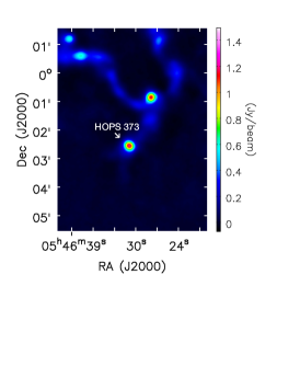
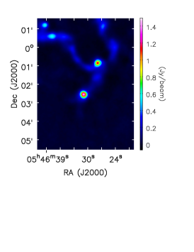
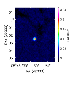
Figure 1: SCUBA-2 850 $\mu$m continuum images of HOPS 373 in the quiescent phase (left, coadded from 14 epochs in 2017), in the burst phase (center, coadded from 12 epochs in 2020–2021), and the residual (burst minus quiescent) image (right).

In this paper, we dissect the ongoing, modest accretion outburst of HOPS 373 as seen in near-IR, mid-IR, sub-mm, mm, and cm observations. The central protostar has characteristics that are typical of a very young protostar driving a powerful outflow. The protostellar envelope of HOPS 373 was initially identified in sub-mm mapping of NGC 2068 (distance of 428 pc, Kounkel et al., 2018) in the Orion B cloud complex (Phillips et al., 2001; Johnstone et al., 2001; Motte et al., 2001), following the discovery of a large CO outflow (Gibb & Little, 2000) and a nearby maser (Haschick et al., 1983). From fits to the near-IR through mm spectral energy distribution, the protostar has a bolometric luminosity of $5.3-6.1$ L_⊙ and a bolometric temperature of $37$ K (Kang et al., 2015; Furlan et al., 2016). The SED, with a total-to-submm luminosity ratio of 34, is red enough to be a PACS Bright Red Source (Stutz et al., 2013) and consistent with an early stage of a Class 0 protostar. HOPS 373 and its associated outflows are not detected in X-rays (Getman et al., 2017). The central object was resolved with high-resolution mm interferometry into two distinct mm peaks separated by $3\farcs 6$, or 1500 AU (Tobin et al., 2015, 2020b). The source drives a powerful outflow. Sub-mm CO emission from the large-scale outflow extends over $1$ arcmin to both the blue (southeast) and red (northwest) directions with a dynamical time of $10^{4}$ yr (Mitchell et al., 2001; Nagy et al., 2020). Far-IR spectra reveal excited molecular emission that likely traces the walls of an outflow cavity (Tobin et al., 2016), with far-IR CO emission that is the brightest of all PACS Bright Red Sources and amongst the brightest of all low-mass protostars (Manoj et al., 2016; Karska et al., 2018).

The NGC 2068 star-forming region, including HOPS 373, has been monitored in the sub-mm by the JCMT Transient Survey since December 2015 (Herczeg et al., 2017). Beginning in 2016, HOPS 373 had gotten fainter by 10% (Johnstone et al., 2018) and stayed steady in this lower luminosity state until a brief increase of 25% in late 2019 (Lee et al., 2021), a pattern also seen at $4.5$ $\mu$m with NEOWISE (Contreras Peña et al., 2020; Park et al., 2021). We report that HOPS 373 has since returned to the bright state in the sub-mm, and analyze in detail the location of emission across the spectrum. We combine the sub-mm lightcurve with near-IR spectroscopy and imaging to dissect how the source is seen across a range of diagnostics. In Section 2, we describe the array of observations that are used in this paper. In Section 3, we describe the sub-mm and NEOWISE lightcurves and provide a physical interpretation for the sub-mm variability. In Section 4, we describe the morphology of the emission sources. In Section 5, we present Gemini/GNIRS spectra to demonstrate the dominance of H₂ emission in the $K$-band imaging. In Section 6, we interpret these results and discuss their importance in on-going and future searches for variable protostars.

2 Observations

2.1 Sub-mm Monitoring at 450 and 850 $\mu$m

The JCMT-Transient survey (Herczeg et al., 2017) has been using SCUBA-2 (Holland et al., 2013) on the James Clerk Maxwell Telescope (JCMT) to monitor every month emission at 450 and 850 $\mu$m from eight regions, including NGC 2068, beginning in December 2015. We also include an earlier data point from the JCMT-Gould Belt Survey (Kirk et al., 2016) obtained from 2014 November 16-22, reported and re-analyzed by Mairs et al. (2017a). In November 2019, we discovered that HOPS 373 had brightened and increased our observational cadence of NGC 2068 to once every two weeks (Figure 1).

Table 1: Selected sub-mm peak brightness^a

MJD	450b	850b	MJD	450b	850b
	[Jy/beam]			[Jy/beam]
57403.348	5.07	1.31	58850.285	5.32	1.32
57424.223	4.91	1.32	58872.391	5.14	1.27
57505.215	4.54	1.23	58915.297	4.99	1.26
57997.668	4.75	1.22	59072.633		1.42
58025.621	4.26	1.19	59087.645	6.21	1.47
58095.422	4.89	1.18	59106.723	6.09	1.48
58133.410	4.35	1.20	59155.480	6.07	1.46
58486.270	4.38	1.19	59180.371	6.22	1.43
58519.336	4.73	1.23	59256.199	5.96	1.44
58580.258		1.26	59275.273	6.08	1.46
58715.621		1.35	59300.223	6.47	1.52
58752.539		1.48	59321.219	6.69	1.57
58774.727	6.02	1.41	59454.633	6.31	1.45
58788.465	5.75	1.40	59485.562	5.81	1.48
58836.355	5.58	1.34	59541.398		1.41
aFull table available online, selected points shown here
bError of 5% at 450 $\mu$m, 2% at 850 $\mu$m

Table 2: Mid-IR Photometry from NEOWISE

MJD	$W1$	Err	$W2$	Err
	[mag]	[mag]	[mag]	[mag]
55266.88a	15.32	0.27	10.930	0.021
55458.14a	15.49	0.38	10.933	0.026
56731.57	15.01	0.24	10.765	0.031
56923.07	15.32	0.50	10.802	0.040
57090.68	14.99	0.24	10.741	0.029
57284.77	15.13	0.42	10.745	0.036
57285.24	15.12	0.25	10.772	0.024
57449.77	15.08	0.26	10.768	0.038
57649.51	15.29	0.30	10.867	0.037
57814.28	15.49	0.40	10.942	0.036
58016.13	15.52	0.42	10.954	0.040
58171.58	15.38	0.36	10.983	0.035
58380.29	15.44	0.35	10.966	0.032
58537.98	15.38	0.33	10.905	0.031
58744.87	14.49	0.15	10.602	0.033
58902.25	15.09	0.24	10.835	0.035
59111.60	14.31	0.14	10.515	0.036
aALLWISE photometry from Cutri et al. (2021)

Table 3: Selected $K$-band Photometry^a

MJD	Brt	Err	Tail	Err	$t_{exp}$
	[mag]	[mag]	[mag]	[mag]	[s]
51093.310	$15.22\pm 0.16$		summed 2MASS $K_{S}^{b}$
55164.335	$15.037\pm 0.029$		summed VISTA $K_{S}^{c}$
55984.308	15.74	0.02	16.26	0.03	72
56262.376	15.67	0.03	16.09	0.04	72
57990.635	15.67	0.02	16.32	0.03	72
58566.254	15.70	0.03	16.28	0.05	72
58812.650	15.67	0.02	16.25	0.03	72
58814.551	15.67	0.02	16.25	0.03	72
58818.513	15.71	0.03	16.28	0.04	72
59075.633	15.63	0.02	16.03	0.03	72
59103.641	15.61	0.02	16.11	0.02	72
59105.629	15.59	0.02	16.14	0.03	72
59100.576	15.62	0.02	16.15	0.02	360
59105.588	15.62	0.02	16.16	0.02	360
59114.569	15.61	0.02	16.11	0.02	360
59118.632	15.59	0.02	16.11	0.02	360
59122.538	15.59	0.02	16.14	0.02	360
59132.591	15.60	0.02	16.10	0.02	360
59136.594	15.57	0.02	16.07	0.02	360
59144.565	15.57	0.02	16.10	0.02	360
59161.540	15.59	0.02	16.07	0.02	360
59172.479	15.57	0.02	16.05	0.02	360
59229.241	15.55	0.03	16.05	0.03	360
59247.368	15.57	0.03	15.97	0.03	360
59257.290	15.62	0.02	16.08	0.02	360
59277.303	15.55	0.02	15.96	0.02	360
59295.228	15.49	0.02	15.85	0.02	360
59436.638	15.48	0.02	15.86	0.03	72
59451.640	15.51	0.02	15.87	0.02	72
59477.540	15.51	0.02	15.92	0.03	72
aFull table available online, selected points shown here.
bIncludes bright compact object and tail.
cExtended source extraction with $5\farcs 7$ diameter aperture
from McMahon et al. (2013).

JCMT Transient Survey observations occur only when the precipitable water vapor content is $<2.58$ mm (opacity of $<0.12$ at 225 GHZ), corresponding to JCMT weather bands 1–3. Because of telluric absorption, the 450 $\mu$m imaging is only useable from the $\sim 50\%$ of our observations that occur during epochs with the lowest precipitable water vapor content.

A full description of the data, advanced reduction, relative alignment, and calibration process developed by the JCMT Transient Survey is provided by Mairs et al. (2017b) for the 850 $\mu$m data and by Mairs et al. (in prep) for 450 $\mu$m data. For HOPS 373, a bright sub-mm source, the relative flux calibration is typically accurate to 2% at 850 $\mu$m and $\sim 5$% at 450 $\mu$m. The effective beam sizes are $14\farcs 1$ and $9\farcs 6$ at 850 and 450 $\mu$m, respectively (Dempsey et al., 2013; Mairs et al., 2021).

The absolute alignment of the SCUBA-2 images is uncertain by $\sim 2^{\prime\prime}$. Six objects in the field are compact, bright enough for centroid, and have a well-identified WISE or 2MASS counterpart. The position of HOPS 373 is shifted to the average WISE position of those objects, with a standard deviation in the positional differences of $1\farcs 4$. However, possible systematics across the field limit our confidence to $2^{\prime\prime}$.

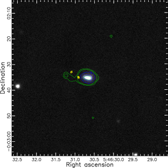
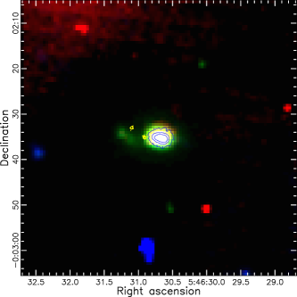
Figure 2: A $1^{\prime}\times 1^{\prime}$ field around HOPS 373 from (left) UKIRT $K$-band imaging and from (right) Spitzer/IRAC imaging in Band 1 (3.6 $\mu$m; blue), Band 2 (4.5 $\mu$m; green) and Band 4 (8 $\mu$m; red). Both images also show blue contours (99.9, 99.8, 99.5 percentiles) from UKIRT 2.122 $\mu$m H₂ imaging and the yellow contours (99.5, 99.0) from emission in the ALMA 890 $\mu$m continuum map; the left image shows green contours (99.9, 99, 98.5) from Spitzer IRAC 4.5 $\mu$m imaging.

2.2 Mid-IR Imaging from 3–24 $\mu$m

The Wide-field Infrared Survey Explorer (WISE) (Wright et al., 2010) surveyed the entire sky in four bands, $W1$ (3.4 $\mu$m), $W2$ (4.6 $\mu$m), $W3$ (12 $\mu$m), and $W4$ (22 $\mu$m), with the angular resolutions of 6$\farcs$1, 6$\farcs$4, 6$\farcs$5, and 12″, respectively, from January to September 2010. After the depletion of hydrogen from the cryostat, the NEOWISE Post-Cryogenic Mission (Mainzer et al., 2011, 2014) has been observing the full sky in $W1$ and $W2$ at a 6-month cadence since late 2013. HOPS 373 has been observed in March and September each year from 2014–2020.

Each epoch consists of $\sim 10-20$ exposures taken over a few days. Each set of exposures are averaged to produce a single photometric point per epoch (following Contreras Peña et al., 2020). No significant variability is identified within each epoch.

We identify consistent seasonal offsets in the NEOWISE position of HOPS 373, as observed during fainter epochs. In March, the average position in $W1$ is located $0\farcs 109\pm 0\farcs 018$ west and $0\farcs 152\pm 0\farcs 016$ south of the average position in September; for $W2$ the September position is $0\farcs 120\pm 0\farcs 016$ west and $0\farcs 149\pm 0\farcs 016$ south. The average standard deviation in the seasonal position in a filter is $0\farcs 024$ in each direction, which we adopt for the uncertainty in individual measurements. We are not aware of the reason behind these seasonal differences or whether they are common.

The field of HOPS 373 was observed multiple times using Spitzer space telescope and the Infrared Array Camera (Fazio et al., 2004) in the IRAC bands 1, 2, 3 and 4, centered at 3.6, 4.5, 5.8 and 8 $\mu$m, respectively. We obtained and averaged IRAC images from three AORs (4105472, 4105728 and 4105984) from the Spitzer Heritage Archive. Figure 2-right shows a color composite image in a $1^{\prime}\times 1^{\prime}$ field extracted from the averaged images in Band 1 (blue), Band 2 (green) and Band 4 (red). The near-IR counterpart of HOPS 373 has excess IRAC Band 2 emission, consistent with classification as an extended green object (EGO; Cyganowski et al., 2008).

The Spitzer/MIPS scan map observing mode covered the NGC 2068 region on 2004 March 15. We obtained the MIPS images at 24 $\mu$m, with the AOR of 4320256 from the Spitzer Heritage Archive.

2.3 Far-IR Imaging from 70–160 $\mu$m

The Herschel Space Observatory (Pilbratt et al., 2010) surveyed protostars in Orion star forming regions (Stutz et al., 2013) with PACS 70 $\mu$m and 160 $\mu$m photometry. The PACS 70 $\mu$m and 160 $\mu$m data of HOPS 373 were acquired over 8′$\times$ 8′  field size with beam sizes of 5$\farcs$6 and 10$\farcs$7, respectively. We obtained the PACS images of HOPS 373 observed on 2010 Sep 28 and 2011 Mar 6 from Herschel science archive with the observation ID of 1342205216, 1342205217, 1342215363, and 13422115364 (Fischer et al., 2020).

2.4 Monitoring at $2.2$ $\mu$m and imaging from 1–2.5 $\mu$m

We monitored HOPS 373 at near-IR wavelengths using the Wide Field Camera (WFCAM; Casali et al., 2007) on the 3.8-m UKIRT telescope from February 2012 to March 2021. WFCAM employs four 2048$\times$2048 HgCdTe Hawaii ii arrays at an image scale of 0$\farcs$4 pixel^-1. The object was dithered to nine positions separated by a few arcsecs, with 2$\times$2 microsteps at each dither position to achieve an image scale of 0$\farcs$2 pixel^-1 in the final mosaics. The observations were obtained using the $J$, $H$ and $K$ MKO filters centered at 1.25, 1.65 and 2.2 $\mu$m respectively, and in a narrow-band filter centered at the wavelength of the H₂ 1–0 S(1) line at 2.1218 $\mu$m. The monitoring comprised of a set of shallow observations (1 s$\times$2 coadds per frame; 72 s integration per mosaic) in $J$, $H$ and $K$ filters from 2012 to 2021 and observations with deeper integration in $K$ (2 s$\times$5 coadds per frame; 360 s integration per mosaic) from September 2020 to March 2021. The magnitudes are derived using the average zero points estimated from a set of isolated point sources, with absolute scaling from images obtained on a clear, photometric night. Data points are discarded if the the standard deviation of the zero points on the derived on field stars is larger than 0.03 mag.

We observed HOPS 373 in the H₂ line on eight epochs. The dither and microstep patter were similar to that in K, but with the per frame exposure time of 40s. This gives a total integration time of 1440 sec for the mosaic from each epoch. The H₂ images are continuum-subtracted using the $K$-band images obtained closest in time and with the best agreement in seeing. The background-subtracted $K$-band image is divided by the average ratio of counts [$K$/H₂] obtained for a few isolated point sources in the $K$ and H₂ images. This image is then subtracted from the background-subtracted H₂ image to obtain the continuum-subtracted emission line image. Since clouds were present during some of those observations, the continuum subtracted images from the different epochs were weighted according to the extinction from clouds and averaged.

The near-IR emission from HOPS 373 consists of a compact source with a tail. The magnitudes for these components, presented in Table 3, are estimated in two apertures of diameter 2″, centered on the compact source at $\alpha$=5:46:30.631 $\delta$=-00:02:35.43 (J2000) and on the tail closer to the YSO, $1\farcs 74$ NE of the first position. Figure 2 shows a 1′$\times$1′ field surrounding HOPS 373 in $K$, generated from the average of the $K$-band images from the epochs with deeper integration. The contours derived from the averaged continuum-subtracted H₂ image are overlaid on the $K$-band image.

We also obtained an acquisition image with Gemini North/GNIRS for our spectrum (Section 2.5). Because HOPS 373 shows extended structure in near-infrared, seven K-band acquisition images were taken to locate the GNIRS slit position precisely. Each image consists of 12 coadded frames with the exposure time of 2 seconds. A blank sky image was generated by combining seven images after masking the emission region; it was then used for background subtraction and flat fielding. The total exposure time of the integrated image is 168 s. The pixel size of 0$\farcs$15 and position angle of $157.49^{\circ}$ were used to put the imaging scale and orientation on the sky.

2.5 Spectroscopy from 1.9–2.5 $\mu$m

We obtained a near-IR $JHK$ spectrum of HOPS 373 using GNIRS on Gemini North in Fast Turnaround Time, program GN-2020B-FT-110 (PI: Doug Johnstone) on 2020 October 3 (HJD=2459126.12). The integration time was 2400 s, split into two ABBA sequences with individual exposures of 300 s.

The data were obtained in the cross-dispersed mode with the 32 mm grating, the short camera, and a 0$\farcs$3 slit to achieve $R=1700$ spectra from 1–2.5 $\mu$m. Our focus here is on the $K$-band spectrum, since little emission is detected in $H$ and none in $J$. The slit of 0$\farcs$3$\times$7″ was aligned with the parallactic angle of $157.49^{\circ}$, almost perpendicular to the direction of the source extension, and centered on the compact source, which dominates the observed emission. The spectra were obtained at an average airmass 1.07. The data were reduced and extracted following standard techniques.

The data were corrected for telluric absorption using B8 V star HD 39803 observed immediately after HOPS 373 at an airmass of 1.14. The flux calibration of the HOPS 373 spectrum, with an estimated synthetic magnitude of $K=15.56$, is estimated by the relative brightness to the same telluric standard star, as measured in the acquisition images, and assuming that the standard star is constant in brightness across the band.

The wavelength solution is accurate to $\sim 0.5$ Å, or 7 km s^-1. However, each pixel covers 80–100 km s^-1, so any asymmetry in spatial extent of the source within the slit may cause additional shifts. We corrected for the local standard of rest (LSR) velocity frame using the IRAF task rvcorrect.

2.6 Radio observations with the VLA

Observations toward HOPS 373 were conducted with the NSF’s Karl G. Jansky Very Large Array (VLA) located on the Plains of San Agustin in central New Mexico, USA. HOPS 373 was observed in multiple bands both before and after the outburst.

2.6.1 C-band Observations at 5 cm

Observations of HOPS 373 were conducted in C-band at a central frequency of 6 GHz on 2015 Oct 06 (2 executions) and on 2015 Oct 07, as part of archival program 15A-369. Both observations were obtained while the array configuration was transitioning from A to D configuration, with 21 useable antennas in the D-configuration. The 2015 Oct 07 data were unusable due to a system issue that occurred during observations. We performed subsequent observations on 2021 Mar 24 (program 21A-409) and 2021 May 15 (program 21A-423) in D-configuration, replicating the setup of the archival observations. In 2015, J0541-0541 was used as the phase calibrator and 3C147 was used as the bandpass and flux calibrator. For 2021, we used J0552+0313 as the complex gain calibrator and 3C147 as the flux and bandpass calibrator.

We reduced and imaged the data using the VLA calibration pipeline in Common Astronomy Software Application (CASA, McMullin et al., 2007) version 6.1.2. The correlator was configured for 3-bit mode where the entire 4 to 8 GHz band is covered with a single setting. We performed additional flagging for system issues (amplitude jumps and spws total swamped with radio frequency interference [RFI]) and re-ran the calibration pipeline. We imaged each observation using the CASA task tclean using robust=0.5 weighting. We also cut out the inner 1.4 k$\lambda$ baselines using the uvrange parameter to remove contributions from large-scale emission associated with the nearby H II region. The 2015 data were self-calibrated to remove dynamic range artifacts associated with a bright source in the field of view. The same source was substantially fainter during the 2021 observations and therefore self-calibration was not required.

For the 2021 observations, we restored the image using the same beam as the archival observations (14$\farcs$77$\times$11$\farcs$40) to perform data analysis with beam-matched data sets. The noise in each observation is 6.28, 5.35, 4.88 $\mu$Jy beam^-1 in respective chronological order.

2.6.2 K-band Observations at 1.3 cm

D-configuration observations were conducted in K-band (22 GHz) on 2015 Oct 17 and 2015 Nov 21 as part of program 15B-229. On 2021 Apr 05 we acquired additional D-configuration observations (program 21A-409). The 2015 observations used 8-bit samplers and observed spectral lines and continuum within two 1-GHz basebands. The main lines targeted were NH₃ (1,1), (2,2), (3,3) and the H₂O (water) maser transition ($J=6_{1,6}\rightarrow 5_{2,3})$) at 22.23507980 GHz. For the follow-up observations in 2021, we used 3-bit samplers to obtain the maximum continuum bandwidth, but also observed the same lines as observed in 2015. We only discuss the water maser emission and continuum data in this paper.

The data were all calibrated using the same methodology as described for C-band. Imaging was performed with the CASA task tclean using robust=0.5 for the continuum data, and robust=2 for the line data with 0.5 km s^-1 channels. The noise in the continuum images is 7.2 and 10.7 $\mu$Jy beam^-1 for the 2015 and 2021 data, respectively, while the noise in the water maser data cubes is 1.23 and 5.55 $\mu$Jy beam^-1 for the 2015 and 2021 data, respectively.

2.6.3 Ka-band Observations at 9 mm

Observations were conducted in C-configuration at Ka-band (33 GHz) on 2016 Jan 30 as part of program 16A-197 and again on 2021 Apr 07 in D-configuration (program 21A-409). Both observations utilized the 3-bit samplers to cover a total bandwidth of 8 GHz, but in 2021 we centered the two 4 GHz basebands at $\sim$29 and 37 GHz to sample a wider fractional bandwidth.

The data were all calibrated using the same methodology as described for C-band. Imaging was performed with the CASA task tclean using robust=0.5 for the D-configuration data observed in 2021. Then for the C-configuration data, we used robust=2.0 and uvtaper=70 k$\lambda$ to better match the D-configuration beam.

2.6.4 Flux Density Measurements with the VLA

To measure the flux densities of the continuum sources in C, K, and Ka-bands, we used the CASA imfit task to fit the source with two Gaussian profiles in K and Ka-bands, where the sources are resolved, and a single Gaussian profile in C-band, where the two sources are unresolved. We provided imfit with initial estimates for the position, flux density, and source size and allowed the fitting to converge on its own. At C-band, we fixed the source size to be a point source.

For the C-band data, we also measured the flux densities of all sources that appeared in both the 2015 and 2021 data since numerous YSOs and background sources lie within the field of view. This enables us to characterize any systematic offsets in flux density calibration. Twenty-five sources detected in both the 2015 and 2021 observations show a median variation of +15 $\mu$Jy, with a corresponding median flux density ratio of 1.22. Similarly, for the two 2021 epochs, 28 matched sources show a median variation of +1 $\mu$Jy, with a corresponding median flux density ratio of 1.01.

The median flux density ratio of 1.22 for the 2015 to 2021 epoch is larger than the expected flux density uncertainty of 5-10% in C-band. Furthermore, the same absolute flux calibrator (3C147) was used for both the 2015 and 2021 observations and the calibrator has had consistent flux density within $\sim$1% between 2016 and 2019. We therefore expect that the large difference of measured flux densities between epochs is due to real variability in the sources and not flux density calibration error.

2.7 ALMA Observations

The Atacama Large Millimeter/submillimeter Array (ALMA), located in northern Chile on the Chajnantor plateau at an elevation of $\sim$5000 m, consists of 50 12 m antennas that constitute the main 12-m array, ten 7 m antennas that form the ALMA Compact Array (also called the Morita Array), and an additional four 12-m antennas that are used for total power observations. The analysis of HOPS 373 makes use of data from standalone observations with the ACA and the 12m array. No data combination is performed.

2.7.1 ACA Observations at 1.33 mm

The Atacama Compact Array (ACA) and Total Power (TP) antennas conducted the Band 6 observation toward HOPS 373 on 2019 March 21 as a part of program (2018.1.01565.S; PI: Tom Megeath). The beam size of the continuum is $4\farcs 4\times 6\farcs 8$ and the reference frequency is 225.69 GHz (1.33 mm). The ¹²CO J=2-1 line (230.538 GHz) analyzed in this work is obtained from the spectral window having the reference frequency of 230.59 GHz and bandwidth of 250.00 MHz. The spectral resolution is 0.317 km s^-1.

Figure 3: Lightcurves of HOPS 373 at 850 and 450 $\mu$m from JCMT/SCUBA-2, at 4.5 and 3.6 $\mu$m from WISE and NEOWISE, and in the $K$-band with UKIRT. The dotted vertical lines mark January 1 for each year. The dashed vertical lines indicate the dates that are used for Table 4.

2.7.2 ALMA 12m Array and ACA Observations at 0.89 mm

The observations of HOPS 373 with the 12m array were conducted as part of program 2015.1.00041.S (PI: John J. Tobin) and were carried out in Band 7 on 2016 September 03, 04, and 2017 July 19. The time on HOPS 373 during each execution was $\sim$20 seconds for a total integration time of $\sim$1 minute. The maximum baseline length for the 2016 and 2017 observations was $\sim$2500 m and $\sim$3700 m, respectively. The correlator was configured to have two basebands observed in low-resolution continuum mode, each baseband having a bandwidth of 1.875 GHz divided into 128 channels that are 31.25 MHz wide. The other two basebands were configured for spectral line observations. The first was centered on ¹²CO ($J=3\rightarrow 2$) at 345.79599 GHz, having a total bandwidth of 937.5 MHz and 0.489 km s^-1 channels. The second spectral line baseband was centered on ¹³CO ($J=3\rightarrow 2$) at 330.58797 GHz, having a total bandwidth of 234.375 MHz and 0.128 km s^-1 channels. The line-free regions of the spectral line basebands were also used in the continuum imaging to result in an effective bandwidth of $\sim$4.75 GHz at 0.89 mm. Reduction of the raw data and subsequent imaging was performed using CASA version 4.7.2. Self-calibration was also performed on the continuum data to increase the S/N, and the self-calibration solutions were also applied to the spectral line data. The resultant 0.89 mm continuum image created using the CASA task clean with robust=0.5 has a beam of $\sim$0$\farcs$11 and a noise of 0.27 mJy beam^-1. The ¹²CO ($J=3\rightarrow 2$) image was created using natural weighting, but the visibilities were also tapered, starting at 500 k$\lambda$ to increase sensitivity to large scale structures, resulting in a $\sim$0$\farcs$25 beam with a noise level of 20 mJy beam^-1 (see Tobin et al. 2020b for further details on the observations and data analysis).

The ACA observation is conducted on 2018 October 2 as a part of program 2018.1.01284.S (PI: Tom Megeath). The continuum is observed with the beam size of 5$\farcs$0$\times$2$\farcs$9 at reference frequency of 338.239 GHz.

2.8 Gaia Astrometry of the Parent Association

HOPS 373 is likely associated with the NGC 2068 - 1 group described by Kounkel et al. (2018) from Gaia DR2 astrometry, located at 428 pc (Gaia Collaboration et al., 2018). The mean proper motion of this group is 0.254 mas/yr in right ascension and -0.573 mas/yr in declination. This proper motion leads to spatial offsets of $\sim$ 0$\farcs$01 between the 2MASS epoch and later epochs from ALMA and NEOWISE. This offset is negligible for our analysis and is not applied to our astrometry. The velocity relative to the local standard of rest ($v_{lsr}$) is $\sim 10.3$ km s^-1 (e.g. Mitchell et al., 2001; Kang et al., 2015; Nagy et al., 2020).

3 Lightcurves of spatially unresolved emission

In this section, we describe the time variability of HOPS 373 and present a fiducial model to explain the sub-mm brightening as a response to increased accretion luminosity from a protostar deeply embedded in an envelope.

3.1 Qualitative and Quantitative Description of the Lightcurves

The burst was initially detected in monitoring at 850 $\mu$m (Figure 1), triggering the follow-up investigation analyzed here. Figure 3 and Tables 1–3 present lightcurves for HOPS 373 in the sub-mm, mid-IR, and near-IR. Figure 4 and Table 4 compare the size of the burst in each band.

Starting in December 2015, HOPS 373 had an initial flux density of $1.3$ Jy/beam at 850 $\mu$m for a few months, before decaying to a steady local minimum (quiescent) level of $1.2$ Jy/beam by April 2016. An early point from the Gould Belt Survey in November 2014 (Mairs et al., 2017a) is consistent with the initial level in December 2015. HOPS 373 then brightened by 25% to 1.5 Jy/beam in September 2019 and decayed back to quiescence by 7 March 2020. By the next data point, in August 2020, HOPS 373 was again bright and has stayed in this bright state in all epochs through the end of 2021. The SCUBA-2 450 $\mu$m data are noisier and sparser but follow the same trend as the 850 $\mu$m measurements, with $F_{450}\propto F_{850}^{1.6\pm 0.1}.$

The late 2019 outburst is narrower and more peaked in time than a Gaussian profile. The rise time is very uncertain and can be arbitrarily steep, since only one point is clearly in the increasing part of the lightcurve. If the rise is exponential, the timescale near the peak must be shorter than 70 days (doubling time shorter than 50 days), based on the peak flux plus the one point in the rise. The decay is better constrained, with an e-folding timescale of $105^{+35}_{-21}$ days (halving time of 73 days). The brightening of 30% from minima to maxima is the third largest change in flux seen in the JCMT Transient survey to date, surpassed by only by HOPS 358 and Serpens Main EC 53 (Lee et al., 2021).

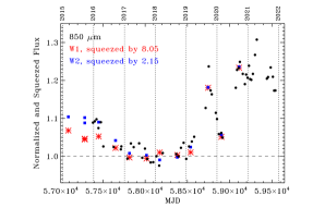
Figure 4: The sub-mm and WISE lightcurves of HOPS 373. The WISE W1 (red asterisks) and W2 (blue squares) photometry is squeezed so that the change between the quiescent level and the most recent burst match the contemporaneous sub-mm fluxes (black circles). The dotted vertical lines indicate January 1 for each year.

The NEOWISE mid-IR lightcurves also follow the same general pattern, with a lower cadence of one epoch every six months. The 2015–2016 decay occurred from a previous stable period that was 25% brighter in $W1$. HOPS 373 then stayed faint until February 2019, with a bright epoch in September 2019, a faint epoch in March 2020, and then another bright epoch in September 2020. The NEOWISE epoch in late 2019 occurred about 8 days before the first SCUBA-2 peak, including one exposure just 4 days earlier. In 2020, the mid-IR returned to quiescence and then burst again, with an epoch four days after a SCUBA-2 observation. The two mid-IR bright measurements are 2.46 and 2.88 times brighter than quiescence at $W1$ but only 1.39 and 1.51 times brighter than quiescence at $W2$.

The $K$-band monitoring is consistent with the sub-mm and mid-IR lightcurves, but with the scale of variability suppressed. Prior to the first burst, the $K$-band emission showed stochastic fluctuations within a 0.1 mag range that are consistent with a constant brightness. The $K$-band monitoring missed the first burst. The most recent points are $\sim 0.15-0.25$ mag brighter than those in quiescence.

The sub-mm and mid-IR lightcurves follow each other closely, but with differences in the amplitude of change. Averaging the two bursts and comparing against the mean of the preceding quiescent period (Table 4), the minimum to peak increase is a factor of 2.66 ($1.06$ mag) at W1, 1.45 (0.40 mag) at W2, and 1.24 (0.23 mag) at 850 $\mu$m. Scaled to the 850 $\mu$m observations, both the $W1$ and $W2$ emission increased more during the 2020 peak than in the 2019 peak. However, this difference may be the consequence of the offset in time between the mid-IR and sub-mm observations in the first burst. The higher cadence of sub-mm observations and the long duration at a near-constant flux during the second burst makes the relative changes more reliable.

The previous Spitzer photometry is consistent with the WISE photometry, with IRAC Band 1 of $13.86$ and IRAC Band 2 of 10.79 mag (Stutz et al., 2013; Getman et al., 2017).

Table 4: Flux versus wavelength^a

MJD=	57750–58450	58748		59111b
$\lambda$ ($\mu$m)	Quiescent	Burst 1	Ratio	Burst 2	Ratio
2.2 compc	3.42e-4	–	–	3.72e-4	1.087
2.2 tailc	1.97e-4	–	–	2.30e-4	1.170
3.6	2.02e-4	4.96e-4	2.46	5.82e-4	2.88
4.5	7.10e-3	9.87e-3	1.39	10.7e-3	1.51
450	4.30	–	–	5.91	1.37
850	1.20	1.485	1.24	1.490	1.24
aAll fluxes in Jy; ratios are burst/quiescent flux.
bRelative offsets from MJD=59111 may be more reliable,
SCUBA-2 averaged from MJD 59107 and 59121.
cCompact source and tail in $K$-band.

3.2 A Fiducial Model for the Sub-mm Lightcurve

The variability in the sub-mm lightcurve is likely a response to a luminosity change within the deeply embedded protostar. The variable emission at 850 $\mu$m, where the envelope is optically thin, is the consequence of a change in the dust temperature within the dense enshrouding envelope (see for example, Johnstone et al., 2013). Infrared wavelengths are closer to the peak of the spectral energy distribution and should directly trace the emission from the protostar and inner disk, but with interpretations that are complicated by uncertain optical depth effects, including scattering. As we will show in Section 4, for this deeply embedded source, the outflow cavity is the surface of last emission for the energy that escapes in the mid-IR, although that energy should trace changes in the emission from the central protostar and its disk.

For sufficiently low dust temperatures, the 450 $\mu$m emission is somewhat shortward of the Planck function Rayleigh-Jeans limit, such that small temperature changes result in larger than linear brightness response. In contrast, the longer wavelength 850 $\mu$m emission is always closer to the Rayleigh-Jeans limit. Indeed, for a mean dust temperature in the envelope of 10 – 15 K at quiescence, the observed relationship between the sub-mm brightnesses, $F_{450}\propto F_{850}^{1.6}$, is well recovered, as the heating leads to a larger response at 450 $\mu$m versus 850 $\mu$m.

Along with the variation in the amplitude of brightness changes across wavelengths to underlying protostar luminosity changes, the Johnstone et al. (2013) model predicts a time delay for the sub-mm emission due to the finite light propagation that is required for the dust heating within the envelope. The crossing time of a 5000 AU core is about 30 days. Given that most of the core mass is on large scales, Johnstone et al. (2013) anticipated a smoothing of the light curve on timescales shorter than a month.

To roughly estimate the sub-mm lightcurve, we model the time-dependent sub-mm transport of energy through the envelope as a response to a jump in protostellar luminosity. Because the expected density and temperature profiles within the core decline as radial power-laws outward from the centre, the sub-mm time response is not uniform but rather highly peaked toward the first few days and with a long tail reaching out to months (heating the backside of the core introduces twice the delay from light travel time). Using this time dependent response to fit the observed sub-mm lightcurve in late 2019, we find that the limit on the exponential rise doubling time of the source shrinks to less than 30 days while the $\sim 75$ day decay halving time stays the same. The timing of the underlying burst, however, is shifted earlier by about 25 days. This is not the entire story, however, as the sub-mm response is approximately a dust temperature response and thus the underlying protostar luminosity change should be much stronger (i.e. expected to be more similar to the $W1$ lightcurve; Johnstone et al., 2013; Contreras Peña et al., 2020). We therefore expect that the protostellar luminosity change during the burst event was significantly more peaked than that seen in the sub-mm, with a half-maximum width of only days for the rise and weeks for the decay.

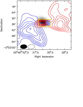
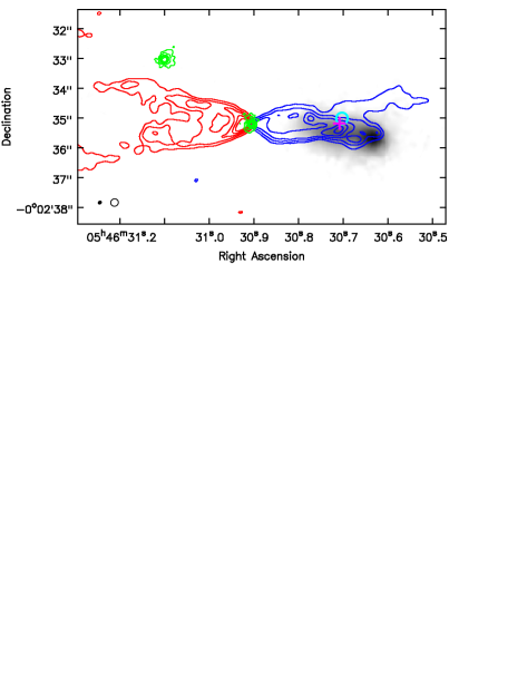
Figure 5: Left: ¹²CO (2-1) integrated intensity map (blue contours from $-6.2$ to $9.0$ km s^-1, red contours from 12.5 to 36.0 km s^-1) overlaid on the 1.3 mm continuum image (grayscale). The contour levels are from 4$\sigma$ to 28$\sigma$ in steps of 4$\sigma$, with 1$\sigma$ = 2.4 Jy beam^-1 km s^-1. The cross (magenta) and circle (cyan) marks show the median centroid of the WISE observations at the quiescent and burst phases respectively. The yellow box is the field of view of the right panel. Right: ¹²CO (3-2) integrated intensity and the 0.89 mm continuum maps overlaid on the Gemini North/GNIRS K-band acquisition image. The blue and red contours show the CO integrated emission over the velocity ranges of from -16.0 to 9.0 km s^-1 and 13.0 to 37.0 km s^-1, with contour levels from 4$\sigma$ to 20$\sigma$ in the step of 4$\sigma$ with 1$\sigma$ = 0.2 Jy beam^-1 km s^-1. The green contours show 0.89 mm continuum emission associated with NE and SW sources with levels of 5$\sigma$ $\times$ (1, 2, 4, 6, 10, 20) with 1 $\sigma$ = 4.0$\times$10^-4 Jy beam^-1. The filled and open circles at bottom left present the beam size of the continuum and spectral line observations, respectively.

4 Morphology of emission components

In the previous section, we demonstrate that HOPS 373 is variable in the mid-IR and sub-mm and interpret the sub-mm variability in terms of an accretion burst. In this section, we dissect the source into distinct structures to understand the variability. In the sub-mm, HOPS 373 has been resolved into two compact continuum sources with a small-scale CO outflow from the SW component (Figure 5). These structures together serve as benchmarks for interpreting the emission sources across wavelengths (Figure 6). In this section, we first describe the binary components and the outflow, and then describe the locations of emission in different bands.

For each instrument and image, the precise location of the emission related to HOPS 373 is determined by centroiding nearby compact sources (Table 5). The absolute images are then registered to the WISE astrometric frame. Appendix A describes the details of these positional shifts.

Table 5: Centroid positions

Instrument	$\lambda$	RAa	Deca
		05 46 00 +Xb	-00 02 00 -Yb
2MASS	$1.2$–$2.5$ $\mu$m	30.648	35.02
WISE	$3$–$25$ $\mu$m	30.705	35.23
IRAC	3.6 $\mu$m	30.686	35.26
IRAC	4.5 $\mu$m	30.692	35.26
IRAC	5.8 $\mu$m	30.709	35.16
IRAC	8.0 $\mu$m	30.698	35.07
MIPS	24 $\mu$m	30.726	35.10
PACS	70 $\mu$m	30.859	35.31
PACS	160 $\mu$m	30.855	34.87
SCUBA-2	450 $\mu$m	30.902	34.17
SCUBA-2	850 $\mu$m	30.913	34.43
ALMA ACA	1.33 mm	30.973	34.11
aFor uncertainty of centroid positions, see Appendix A
bAs example, the first source is 05 46 30.648 -00 02 35.02

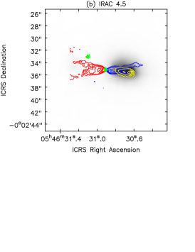
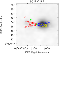
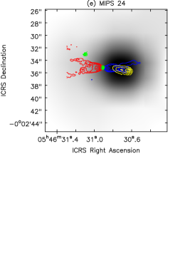
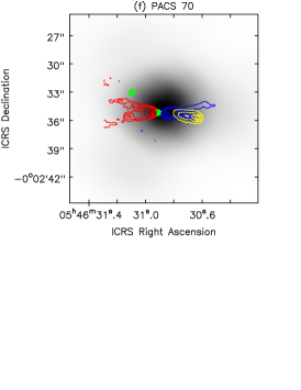
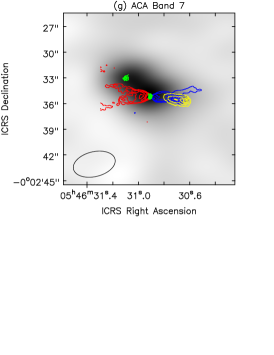
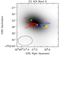
Figure 6: The ¹²CO 3-2 (blue and red contours, following Figure 5), 0.89 mm continuum emission (green) and GNIRS Ks-band contours (yellow) map, superimposed on (a) IRAC 3.6 $\mu$m (Band 1) image; (b) IRAC 4.5 $\mu$m (Band 2) image; (c) IRAC 5.8 $\mu$m (Band 3) image; (d) IRAC 8 $\mu$m (Band 4) image; (e) MIPS 24 $\mu$m band image; (f) PACS 70 $\mu$m band image; (g) ACA Band 7 (0.89 mm) continuum image ; (h) and ACA Band 6 (1.3 mm) continuum image.

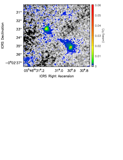
Figure 7: ALMA Band 7 (0.89 mm) continuum image of HOPS 373. The NE and SW sources show a weak extended continuum emission surrounding the compact emission.

4.1 Binarity in the sub-mm

High-resolution mm imaging shows two distinct continuum sources with a separation of $3\farcs 6$ and a position angle 232^∘ (Figure 7, Tobin et al., 2015, 2020b), using the NE component as the reference point. The continuum sources seem to be surrounded by a large envelope, which is resolved out in the high-resolution image. In Figure 7, the diffuse emission surrounding the sources is associated with this unseen larger envelope.

The binary components of the 0.89 mm emission are HOPS 373 NE centered at 05:46:31.100 -00:02:33.02 and HOPS 373 SW at 05:46:30.905 -00:02:35.20 (Tobin et al., 2020b). The integrated flux of the NE and SW sources are 85.0$\pm$3.3 mJy and 81.8$\pm$1.7 mJy, respectively, as measured from the integrated flux in a 2D Gaussian fit of imfit in CASA. The total 0.89 mm emission in the two continuum sources is $\sim 0.17$ Jy, or about 9% of the integrated flux in the 850 $\mu$m emission seen in SCUBA-2. Most of the emission is resolved out with the small beam.

The ACA 1.33 mm continuum emission, obtained with a 6$\farcs$8$\times$4$\farcs$4 beam, has a centroid of 05:46:30.971 -00:02:34.13, between the two compact components, is elongated in the position angle of those components, and has a flux of 362$\pm$9 mJy. In the Rayleigh-Jeans limit, this flux at 1.33 mm implies a flux of 886 mJy at 850 $\mu$m, or 45% of the total emission from the source. In a simulation of the ACA observation, if only the two point sources are present, they would be marginally resolved. However, the ACA continuum image shows an emission peak between the two sources, which requires some diffuse emission surrounds the two compact sources.

During the burst, the centroid of the residual (burst–quiescent) emission in the SCUBA-2 850 $\mu$m images is located $1\farcs 1$ closer to the SW component than the quiescent emission, consistent with expectations if the SW component is the source of the variability. The residual emission also has a compact profile, consistent with a FWHM of $\sim 7\arcsec$, while the quiescent emission has a FWHM of 15″ in the SCUBA-2 data.

4.2 CO Outflows

The ALMA images from the ACA and the 12 m array reveal large-scale outflows in CO 2–1 emission (see Figure 5 and also channel maps from the high-resolution 12m array observations of the CO outflow presented in Appendix A). At large scales, the blueshifted outflow is located to the southeast of the source while the redshifted outflow is located to the northwest (see also Mitchell et al., 2001; Nagy et al., 2020). At small scales, the outflow direction is the opposite: the blueshifted outflow is launched to the west, while the redshifted outflow is launched to the east. The small-scale outflow is driven by the southwestern component.

The position-velocity (PV) diagram (the upper panel in Figure 8) along the position angle of 90^∘ centered on HOPS 373 SW shows that the blue and redshifted outflows extend to 4″ from the source. CO emission is also detected in extremely high-velocity components, or bullets, in a jet-like collimated morphology with velocities of $-60$ and 65 km s^-1 in each direction, relative to the source velocity of 10 km s^-1(the lower panel in Figure 8). Such bullets are commonly detected in CO emission in jets from very young protostars (Tychoniec et al., 2019). However, since the CO (3-2) line observation was carried in 2016, the jet-like feature is not directly related to the recent outburst.

The northeastern component is not associated with any detected small-scale outflow. Any outflow from the northeastern component would have to either be low-velocity and absorbed by the cloud or large enough that it is resolved out. The large-scale outflow is either a historical remnant of an outflow driven by the northeastern component, or the southwestern component has precessed such that the wind direction changed from red to blue. A large change in outflow direction has been identified in another very young protostar, IRAS 15398-3359 (Okoda et al., 2021).

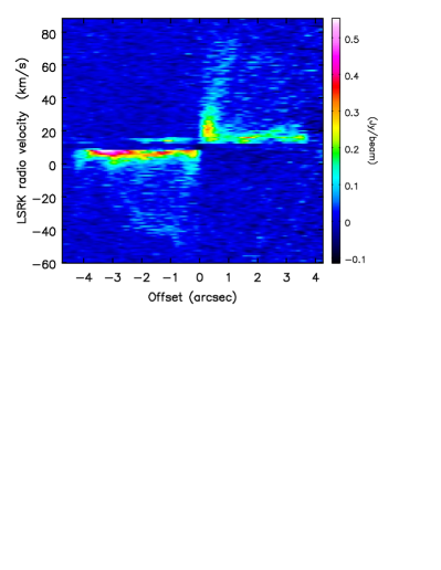
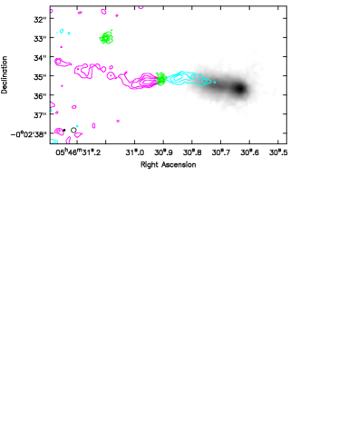
Figure 8: Top: Position-velocity diagram of CO 3-2, centered at HOPS 373 SW and aligned along the outflow axis, with a position angle of 90^∘. Extremely high velocity bullets are detected within $1\arcsec$ of the star in both the red and blueshifted jets. The velocity shown here is not corrected for the source velocity of $\sim 10$ km s^-1. Bottom: ¹²CO (3-2) integrated intensity and the 0.89 mm continuum maps (green contours) overlaid on the GNIRS K-band acquisition image. Cyan and magenta contours show CO emission integrated over the velocity ranges from -50.0 to -17.0 km s^-1 and 38.0 to 75.0 km s^-1, respectively, with contour levels set to (3, 5, 7, and 10) $\times\sigma$, with $\sigma=0.19$ Jy beam^-1 km s^-1.

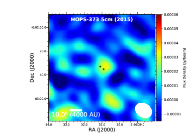
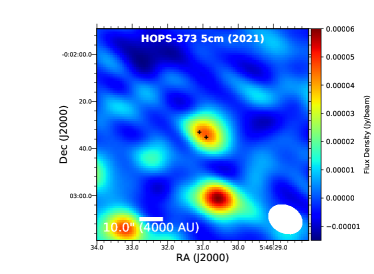
Figure 9: VLA images toward HOPS 373 at 5 cm; the 2015 data are on the left and the 2021 data are on the right. The images clearly show that the 2021 data are brighter at 5 cm, potentially a calibration issue. The positions of the SW and NE compact continuum components of HOPS 373 are marked by crosses in each panel. The beam in each image is 14$\farcs$77$\times$11$\farcs$40.

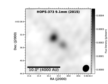
Figure 10: Top: VLA images of HOPS 373 at 9.1 mm in 2015 (left) and 2021 (right). Although both sources appear brighter in 2021, possibly because of absolute calibration error, the ratio of flux densities indicates that the SW source is brighter in 2021. Bottom: VLA images toward HOPS 373 at 1.3 cm with H₂O maser contours overlaid, in 2015 (left) and 2021 (right), both shown with the same color stretch. The positions of the northeast and southwest components of HOPS 373 are marked by crosses. The H₂O maser emission is associated with the southwest source and brightened substantially in 2021 relative to 2015; the contours start at 3$\sigma$ and increase on 2$\sigma$ increments where $\sigma_{2015}=1$ (mJy km s^-1)/beam and $\sigma_{2021}=4$ (mJy km s^-1)/beam demonstrating a 7$\times$ increase in maser emission between 2015 and 2021. The 2015 maser emission is integrated from -15.5 to -14.5 km s^-1, and the 2021 maser emission is integrated from 9.5 to 10.5 km s^-1.

4.3 Radio emission from 0.9–5 cm

The archival observations from the VLA were obtained in 2015 October, just prior to the start of JCMT monitoring. At that time, the protostar was likely in a quiescent state, though brighter than the minimum. Our follow-up C-band observations in 2021 occurred $\sim$6 months after the current and on-going burst began.

Emission at 5 cm: The large VLA beam encompasses both of the distinct sub-mm continuum sources. The flux density of HOPS 373 was 32$\pm$6 $\mu$Jy in 2015 and 47$\pm$6 $\mu$Jy in 2021 (see Table 6), apparently brighter during the burst but consistent with no change to within $2\sigma$. As detailed in Section 2.6.4, there is a systematic offset in the distribution of flux density differences and ratios measured for other sources in the field between 2015 and 2021. Therefore we cannot be confident that the difference in flux density at C-band represents a true variation. These uncertainties also do not include the 5-10% absolute flux density calibration uncertainty.

Table 6: VLA Flux Densities^a

	Flux Density	Flux Density	Flux Density
$\lambda$	2015/2016	2021 Mar/Apr	2021 May
(cm)	($\mu$Jy)	($\mu$Jy)	($\mu$Jy)
0.9	761$\pm$24	960$\pm$30	$\cdots$
1.3	323$\pm$10	337$\pm$38	$\cdots$
5.0	32$\pm$6	47$\pm$6	45$\pm$6
NE
0.9	486$\pm$17	569$\pm$21	$\cdots$
1.3	170$\pm$7	175$\pm$27	$\cdots$
SW
0.9	275$\pm$17	391$\pm$21	$\cdots$
1.3	153$\pm$7	162$\pm$27	$\cdots$
H2O Maser	(mJy km s-1)	(mJy km s-1)
1.349	5.5 $\pm$0.8	56.1$\pm$7	$\cdots$
aMeasured from fits with Gaussian profiles

Emission at 1.3 cm: At 1.3 cm the two continuum sources are marginally resolved when imaged at the same resolution in 2015 and 2021 (Table 6). The NE component appears brighter than the SW at 1.3 cm in 2015, while in 2021 the SW source appears to be the brighter (Figure 10), though with flux densities consistent within the uncertainties.

Emission at 0.9 cm: At 0.9 cm, the NE source is brighter than the SW source in both 2015 and 2021, but the sources are both overall brighter in 2021 relative to 2015 (Figure 10). Using the well-resolved and high S/N detections of each source at 9 mm, we find a NE/SW flux density ratio of 1.77$\pm$0.13 in 2015 and 1.45$\pm$0.12 in 2021, suggesting that the SW source brightened; again a constant ratio cannot be ruled out at the 2$\sigma$ level. Most of the 9-mm emission is produced by thermal dust, so the brighter emission from the SW source indicates an increase in the dust temperature, in agreement with the JCMT sub-mm observations.

Emission in water masers: The water maser emission is only associated with the SW source, with a spatial position that did not change between 2015 and 2021 (Figure 10). The flux density increased by a factor of $\sim$10 from 2015 to 2021 (Table 6) and changed in velocity from -15 km s^-1 in 2015 to $\sim$10 km s^-1 in 2021 (relative to the local standard of rest and not corrected for the source velocity). The maser lines are narrow, with FWHM of $<$1 km s^-1 in both epochs. The previously published single-dish maser observations toward the region detected maser activity at substantially higher flux densities and at velocities of $\sim$20 km s^-1 (Haschick et al., 1983).

4.4 Near- and Mid-IR emission from the outflow

The WISE $W1$ and $W2$ emission is centered $3\farcs 1$ to the west of the ALMA-observed southwestern sub-mm continuum source and is spatially unresolved due to the $\sim 6^{\prime\prime}$ point spread functions. The two epochs when HOPS 373 was bright occurred in Sept. 2019 and Sept. 2020. Compared to the centroid position from previous September epochs, in 2019 the centroid position in $W1$ is $0\farcs 176$ W and $0\farcs 093$ N of previous Sept. epochs; in 2020 the centroid is $0\farcs 122$ W and $0\farcs 077$ N. In $W2$, the offsets are $0\farcs 132$ west and $0.068$ north in 2019 and $0\farcs 133$ W and $0.079$ N in 2020. Based on previous epochs, each position has a $1\sigma$ uncertainty of $0\farcs 025$. These centroid positions include the quiescent emission and the emission added from the burst. After subtracting the quiescent emission, the position of the burst would be even further away from the quiescent centroid.

The $K$-band images of HOPS 373, mostly H₂ emission (see Section 5), are dominated by a compact source 4.2^′′ west of the southwestern continuum component, with a tail of fainter emission extending back to the northeast toward the source (Figure 5). The IRAC 4.5 $\mu$m emission also shows very faint emission to the east of this source, likely associated with the redshifted outflow (Figure 2).

The $K$-band tail follows the southern half of the blueshifted CO emission. The $K$-band compact emission is located just beyond the extent of the CO emission, perhaps indicating a bow-shock at the end of the jet (Varricatt et al., 2010).

The $J$- and $H$-band emission seen with UKIRT is spatially consistent with the $K$-band emission and likely traces molecular and atomic line emission from the outflow. The total source brightness is $J=21.18\pm 0.4$ and $H=18.78\pm 0.09$, but the emission is too faint to divide into individual epochs or to separate into different components. Spezzi et al. (2015) reported $H=19.34$ from the VISTA Orion Survey, fainter than measured here, either because of variability or a smaller aperture over which the emission was measured.

4.5 Far-IR emission from the SW component

The Herschel PACS 70 and 160 $\mu$m emission is nearly centered on the HOPS 373 SW (Figure 6). The binary is not resolved and the emission is not elongated in any direction. The total fluxes at 70 $\mu$m and 160 $\mu$m are 5.46 Jy and 36.3 Jy, respectively (Furlan et al., 2016). The far-IR emission seems to be mainly associated with HOPS 373 SW, attributed to the thermal emission from the HOPS 373 SW envelopes rather than the scattered light from the cavity wall or the shocked emission, seen in shorter wavelengths.

4.6 Summary of source morphology

The HOPS 373 protostar consists of two compact dust sources, HOPS 373 NE and SW, separated by $3\farcs 6$, corresponding to a projected separation of 1500 AU at the distance of 428 pc. Both a molecular outflow and maser emission are associated with the SW component. No small-scale outflow is seen from HOPS 373 NE.

In Figure 6, we identify the location where each emission component is detected. The near- and mid-infrared emission centroids are all consistent with emission located along the blueshifted outflow from the central source, where the opacity should be reduced. At 70 $\mu$m, the emission is located nearly on the position of the SW source. In the ALMA ACA Band 6 imaging at 1.33 mm, the emission centroid is located between the sources, as is the emission at $\sim$850 $\mu$m from SCUBA-2. The NE source does not show any emission feature over the mid-infrared images. However, as the wavelength gets longer through far-infrared to sub-mm, the thermal emission from each individual dust component becomes significant and the flux of the NE source increases.

The variability in the infrared continuum and in the maser emission, along with the detected outflow, conclusively demonstrates that the SW component is the component that is actively accreting and variable. The variability in maser emission is consistent with past associations between maser emission and accretion (e.g. Burns et al., 2015, 2020; Hirota et al., 2021; Stecklum et al., 2021). Assuming that the maser variability is related to the accretion event, then the water masers are responding to the increase in radiation field. The masers may also brighten due to an increase in outflow activity, any such change would occur over longer timescale than observed for HOPS 373 and would mean that the correlation between maser emission and sub-mm emission is only a coincidence.

The NE source is only bright in the sub-mm and is not detected in the mid-IR. The luminosity must be very low. The compact object is the size of a disk, but the central source must be low-mass and is not actively driving any outflow. The large-scale outflow may be a remnant outflow from the NE source or may be an outflow from the SW source that changed direction.

5 Molecular Emission in the Near-Infrared

The compact near-IR emission is located $\sim$4.3″ away from HOPS 373 SW and has $\sim$1″ in diameter. The elongated emission feature extends $\sim$3″ to the east, towards the driving source. We obtained the near-infrared spectrum from the compact source by placing the 0.3″$\times$7″ slit nearly perpendicular to the extended near-IR emission feature (see Figure 5). The near-IR spectrum of the compact $K$-band source is dominated by rovibrational H₂ emission, detected in vibrationally excited lines up to $v=3$ (Figure 11). Table 7 provides the intensities of the H₂ lines, measured from fitting Gaussian profiles to the lines. The flux error is estimated from the standard deviation in the continuum near each line. The H₂ 1-0 S(1) line center is shifted from the central wavelength by about -22 km s^-1 in LSR velocity, or $\sim-32$ km s^-1 relative to the source velocity.

For an optically thin line, the intensity is proportional to the column density $N_{vj}$ in a given rovibrational level as follows

$$\frac{I_{\lambda}(v,J)}{\Omega}=\frac{Ahc}{4{\pi}{\lambda}}N(v,J)\cdot 10^{-0.4A_{\lambda}}$$ (1)

where $I$ is the line flux given in the unit of W cm^-2, $A$ is the Einstein coefficient, $h$ is the Planck constant, $c$ is the speed of light, $N$ is the column density at a given rovibrational level, and $\Omega$ is the area that the emission comes from, with 0$\farcs$3$\times$1″adopted here for simplicity. The near-infrared extinction to the H₂ emission is estimated to be 8.4$\pm$0.1 at 1 $\mu$m from the H₂ line ratio of 1-0 S(1) to 1-0 Q(3) with the extinction law of A_λ/A₁ = $\lambda^{-2.27}$ where A₁ is the extinction at 1 $\mu$m (Maíz Apellániz et al., 2020). Other H₂ line ratios yield $\rm{A}_{1}=4-10$ mag but are less reliable because they rely upon lines at wavelengths that are progressively longward of 2.4 $\mu$m, where our telluric correction is more uncertain. For comparison, if we adopt the extinction law of Wang & Chen (2019), with a near-IR power-law index of 2.07, the H₂ 1-0 S(1) to 1-0 Q(3) line flux ratio would lead to extinctions of $A_{K}=1.5$ mag and $A_{1}=7.8$ mag.

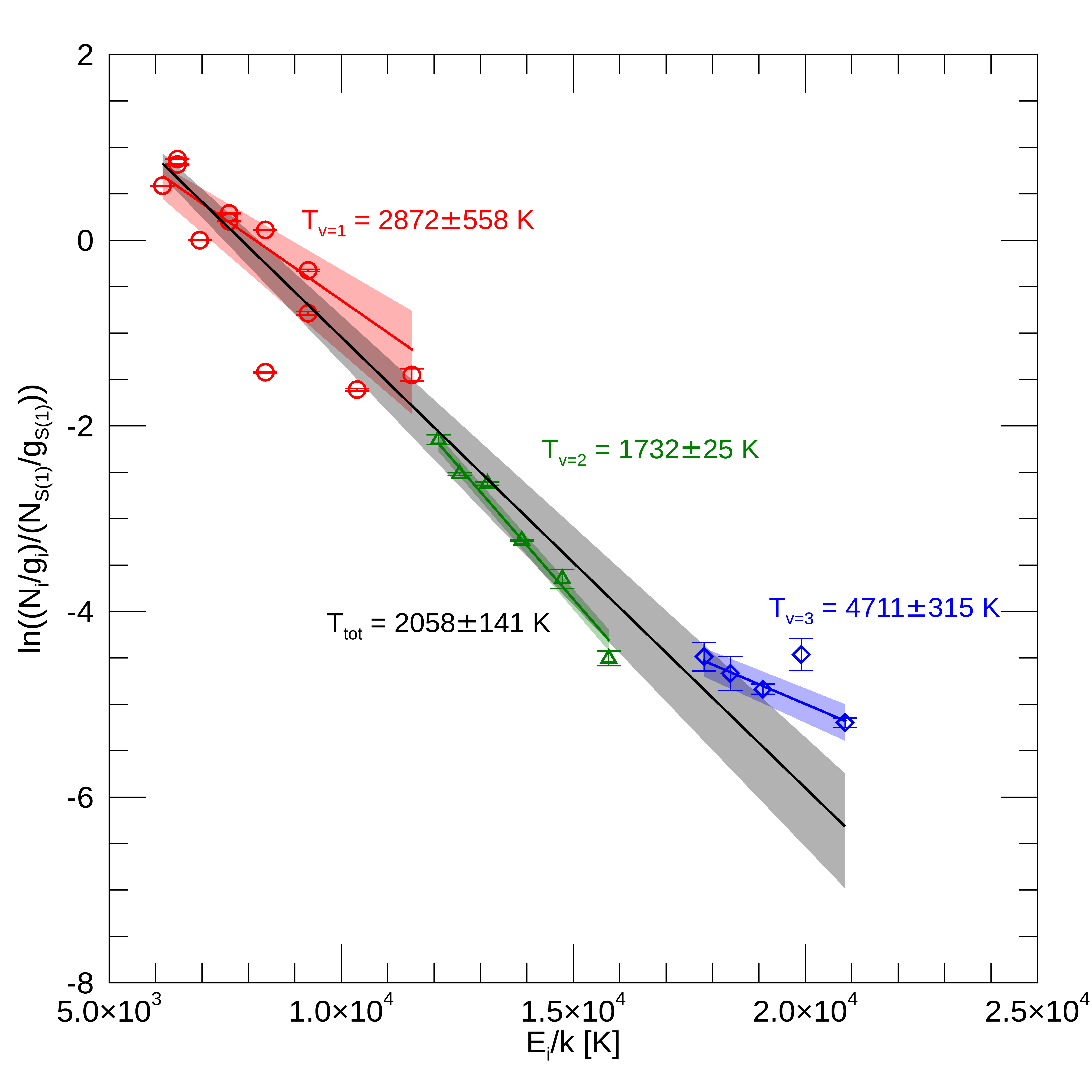
Figure 12: The excitation diagram of H₂ transitions for HOPS 373. The column densities per statistical weights of H₂ transitions are normalized by that of H₂ 1-0 S(1) line. The vibrational transitions of $v$=1-0, 2-1, and 3-2 are fitted by red, green, and blue straight lines, respectively. The H₂ 1-0 Q(5) line is excluded from the fit. The total H₂ transitions are fitted by the black solid line. The shaded regions show the 3 sigma error of the fitted lines.

After correcting for the near-infrared extinction, the H₂ $v$=1-0, 2-1, and 3-2 rovibrational transitions are fitted with the excitation temperatures of about 2900, 1700, and 4700 K, respectively (Figure 12). A combined fit to all lines leads to an excitation temperature of about 2100 K and a total column density of 4.4$\times$10¹⁹ cm^-2 calculated assuming a 0$\farcs$3$\times$1″  emitting area on the sky. These temperatures are roughly consistent with H₂ excitation temperatures from other protostellar jets (e.g. Giannini et al., 2002; Takami et al., 2006; Beck et al., 2008; Oh et al., 2018) and, together with the 1-0 to 2-1 S(1) line ratio of $\sim$8 (Smith, 1995), indicate thermal excitation from shocks. The lines from the $v^{\prime}=3$ are somewhat stronger than thermal excitation, suggesting a possibility that populations in high vibrational levels are enhanced by UV irradiation (e.g. Black & van Dishoeck, 1987; Nomura et al., 2007).

The total flux of H₂ emission in the $K$-band between wavelengths from 2.03 to 2.37 $\mu$m is 4.0$\times$10^-21 W cm^-2, based on the best-fit to all lines. This flux is 12.0 times brighter than the total continuum flux in the K-band, as measured from the spectrum. Extrapolating from an H₂ excitation temperature of 2100 K and column density of 4.4$\times$10¹⁹ cm^-2, extincted by $A_{1}=8.4$ mag, leads to H₂ fluxes of 3.21$\times$10^-20 W cm^-2 in the WISE W1 band and 2.97$\times$ 10^-20 W cm^-2 in the WISE W2 band (magnitudes of 16.8 and 15.8, respectively). Even with some correction for emission outside of the slit, these magnitudes are much fainter than the observed $W1$ and $W2$ brightness.

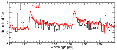
Figure 13: GNIRS CO overtone band spectrum. The IGRINS spectrum of IRAS 03445+3242 (Lee et al., 2016), multiplied by 13, is overlaid with red. The spectrum of HOPS 373 is not continuum-subtracted.

The CO $v$=2-0 and 3-1 overtone bandheads are detected in emission with an integrated flux 50–90 times weaker than the summed H₂ line emission (Figure 13). These lines typically trace emission at $\sim 3000$ K, hotter than either the sub-mm outflow emission seen in the outflow or the warmer far-IR emission (Tobin et al., 2016). The critical density required to excite these levels, $\sim 10^{12}-10^{13}$ cm^-3 (Najita et al., 1996), is associated with dense inner disks and not with outflows.

If the $W1$ and $W2$ variability are both caused by continuum emission that scales in the same way, then $\sim 73$% of the quiescent emission in $W2$ would have to be produced by lines (assuming that the lines are non-variable). Although the H₂ component identified in the $K$-band cannot explain such line emission at $W1$, a cooler H₂ emission component may be present that could contribute flux at $W2$ but not in $W1$ or in the $K$-band (see, e.g., excitation diagrams in Giannini et al., 2006). This scenario would also be consistent with the warm ($\sim 300$ K) CO component detected in the far-IR (Tobin et al., 2016). Alternately, strong shocks may also produce strong CO emission, as inferred in the 4–5 $\mu$m emission in photometry for the outflow shock HH 212 and the young protostar NGC 1333 IRAS 4B (Tappe et al., 2012; Herczeg et al., 2012). Strong CO fundamental ($v=1-0$) band emission has been detected from the outflow of GSS 30 (Herczeg et al., 2011), an embedded protostar that also shows excited far-IR CO emission, like HOPS 373 (Green et al., 2013; Tobin et al., 2016).

Table 7: H₂ Linelist

Line	$\lambda$	Flux	Error
ID	($\mu$m)	($10^{-23}$ W cm-2)
1-0 S(4)	1.8919	67.3	0.9
2-1 S(5)	1.9449	4.7	0.4
1-0 S(3)	1.9576	293.8	0.4
2-1 S(4)	2.0041	3.8	0.4
1-0 S(2)	2.0338	92.0	0.1
3-2 S(5)	2.0656	2.5	0.1
2-1 S(3)	2.0735	16.5	0.1
1-0 S(1)	2.1218	168.7	0.6
3-2 S(4)	2.1280	1.8	0.3
2-1 S(2)	2.1542	8.7	0.1
3-2 S(3)	2.2014	3.7	0.2
1-0 S(0)	2.2233	77.0	0.1
2-1 S(1)	2.2477	21.8	0.3
3-2 S(2)	2.2870	1.3	0.2
2-1 S(0)	2.3556	6.0	0.3
3-2 S(1)	2.3865	3.5	0.5
1-0 Q(1)	2.4066	201.1	0.5
1-0 Q(2)	2.4134	100.2	0.5
1-0 Q(3)	2.4237	173.2	0.6
1-0 Q(4)	2.4375	96.2	0.3
1-0 Q(5)	2.4548	62.7	0.4
1-0 Q(6)	2.4756	46.1	0.9
1-0 Q(7)	2.5000	69.5	1.0
1-0 Q(8)	2.5280	30.5	2.0

Figure 11: The normalized K-band spectrum of HOPS 373. The rovibrational transitions of H₂ dominate the K-band emission. The rovibrational transitions of $v$=1-0, 2-1, and 3-2 are denoted with red, green, and blue labels above the lines.

6 The Dissection of the HOPS 373 Accretion Burst

The broadband wavelength coverage and $K$-band spectroscopy help us to dissect the response to an accretion burst of different structural components in the HOPS 373 protostar. In this section, we step through the different wavelengths to describe the changes in the central source, as seen at long wavelengths, and how some of that emission escapes in the outflow cavity at short wavelengths. We then describe the importance of these results for surveys that search for variable protostars.

6.1 The sub-mm variability and change in luminosity

The sub-mm continuum emission seen with JCMT/SCUBA-2 traces dust in the envelope, heated primarily by emission from accretion onto the central protostar (see Section 3.2). Since the envelope acts as a bolometer, any change in the sub-mm emission should probe changes in the dust temperature profile caused by variable accretion luminosity (Johnstone et al., 2013). The different scales for emission are important: the SCUBA-2 imaging has an angular resolution of $14\farcs 1$ ($\sim$6100 AU), so most of the envelope emission is detected in a single resolution element. The ALMA 12-m Array observations have an angular resolution of $\sim 0.08^{\prime\prime}$, the typical scale of protoplanetary disks, and filter out most of the envelope emission, which occurs on scales larger than $\sim 1^{\prime\prime}$.

In the SCUBA-2 monitoring, HOPS 373 brightens by a factor of $\sim 1.25$ at 850 $\mu$m. The single-dish SCUBA-2 and ACA sub-mm emission is centered between the two sources. The variability is associated with the SW source, as inferred by the location of WISE mid-IR emission, ongoing outflow activity, and increase in H₂O maser emission. In the resolved ALMA observations of the continuum emission at 890 $\mu$m, obtained during a quiescent period of the NEOWISE lightcurve, the SW source is 88% as bright as the NE source. Nevertheless, while the NE component is bright in high-resolution sub-mm images, the images at shorter wavelengths indicate that this source is faint and contributes little to the heating and total luminosity of the envelope. The SW component dominates the emission in the far-IR, where the combined SED peaks (Stutz et al., 2013); the SW component is also not detected at shorter wavelengths.

The bolometric luminosity of $5.3$ L_⊙ (Kang et al., 2015), measured during a low luminosity epoch, corresponds to an accretion rate of approximately

$$\dot{M}_{acc}=1.4\times 10^{-6}\frac{R*}{2\times R_{\odot}}\frac{0.3M_{\odot}}{M_{*}}~{}{\rm M}_{\odot}{\rm yr}^{-1}.$$ (2)

The SW component is expected to contribute most of the envelope heating. With this assumption and scaling from radiative transfer models by Baek et al. (2020), the 25% brightness increase at 850 $\mu$m translates into an increase of the source luminosity by a factor $\sim 1.8$. However, if both targets contribute equally to the source luminosity, and therefore the heating of the envelope (similar to the measured ratio on small scales with ALMA), then we would infer a brightness increase of 50% at 850 $\mu$m from the southwest source. This brightening would correspond to a luminosity increase of a factor of 3.3.

Our monitoring probes only changes during what we identify as the quiescent level of emission. The far-IR CO emission is about 30 times stronger than that expected for its luminosity, based on correlations established for protostellar outflows (Manoj et al., 2016). In addition, HOPS 373 is the only PACS Bright Red source detected in far-IR [OI] and OH emission in the Tobin et al. (2016) sample, indicating the presence of very strong shocks in the outflow.

If the high far-IR CO luminosity is associated with a photo-dissociation region along the outflow cavity walls, then the current internal luminosity must be, higher than that from the SED fitting, given the cooling timescales. Inspecting the SED model of HOPS 373 by Furlan et al. (2016), the model flux peaks at shorter wavelengths than the observed SED. The envelope may be more massive than $\sim 0.3$ M_⊙ (Furlan et al., 2016), since no near- and mid-IR emission is detected from the protostar itself. We estimated the envelope mass from the 850 $\mu$m flux to be $\sim 3.6$ M_⊙ by using equation 1 in Johnstone et al. (2001) with the dust temperature of 20 K and the dust opacity of 0.01 cm² g^-1 at 850 $\mu$m. The source luminosity may be underestimated, if some uncertain fraction of the energy escapes the system through the outflow cavities, although any underestimate would likely be much less than the factor of 30 needed to explain the CO emission.

On the other hand, if the far-IR CO emission is dominated by the shocked gas, then the internal luminosity and far-IR CO emission might not be necessary to be contemporaneous. HOPS 373 is the only one of the PBRS with strong far-IR CO and H₂O lines, along with some OH and [O I] emission (Manoj et al., 2016; Tobin et al., 2016). The ALMA observation of CO emission shows a well-collimated jet and spot-like H₂ emission at along the outer boundary of CO outflows and at the termination of the outflow. These observational results indicate non-dissociative C-shocks, and a time difference of  1000 yrs might be possible in the consideration of shock chemistry. Other young sources, such as NGC 1333 IRAS 4B, HOPS 108, and HOPS 370, also have anomalously strong CO emission, perhaps because the emission is produced by non-dissociative C-shocks (e.g. Herczeg et al., 2012; Manoj et al., 2013; Karska et al., 2018).

6.2 Interpreting the brightness changes in the infrared

The warm dust and gas emission seen in the near- and mid-IR traces the outflow (see schematic from Visser et al., 2012). The H₂ emission is produced in shocks in the outflow and along the cavity walls. The continuum emission, which dominates the $W1$ imaging, is most likely produced by the warm inner disk, which irradiates the cavity walls, although we cannot rule out in situ emission from warm dust that could line the cavity walls. In this scenario, the mid-IR emission from the disk is detected in scattered light off of the cavity walls. The high extinction through the envelope to the central star absorbs all short-wavelength emission, with a dense envelope that causes the SED to peak at $100$ $\mu$m, while the line of sight extinction to the H₂ emission in the outflow is $A_{1}=8.4$ mag. This extinction is caused by dust in the interstellar medium and in the circumstellar envelope. The disk origin for the infrared continuum emission is supported by the detection of CO overtone band emission and by the ratio of changes in the infrared compared with the sub-mm.

The CO overtone bands (${\Delta}v=2$) in our GNIRS spectrum are likely produced in the disk (e.g. Brown et al., 2013; Ilee et al., 2013), since the critical density to excite the upper levels is higher than expected for outflow shocks. The detected CO emission would therefore be seen only because the outflow scatters emission that originates in the disk. This scenario strongly supports the idea that the $W1$ emission is scattered light. For the high-mass protostar, IRAS 11101-5829, CO overtone emission is detected in scattered light by the outflow wall but is generated by the disk (Fedriani et al., 2020). The high-mass protostar S255IR NIRS 3 also seems to have a similar morphology, with variability in continuum and CO emission traced to light echoes (Caratti o Garatti et al., 2017). This specific scenario, with H₂ emission from extended winds and CO emission produced by the disk but seen only in scattered light, also has a direct analog with the post-main sequence, pre-planetary nebula IRAS 16342-3814 (Gledhill & Forde, 2012).

The relation between the variability in W1 and that at 850 $\mu$m, $F_{\rm mid-IR}\propto F_{850}^{\eta}$, is $\eta\sim 4.6$ for HOPS 373, consistent with the empirical correlation found for mid-IR and sub-mm variability for a subset of JCMT Transient Survey embedded protostars, $\eta=5.53\pm 0.29$ (Contreras Peña et al., 2020). This correlation is also close to expectations from radiative transfer models that include mid-IR emission from disks scattering of light off of outflow cavities (Baek et al., 2020).

The variability is smaller in other IR bands, with $\eta\sim 1.8$ at $W2$ and $\eta\sim$0.5 at $K$-band (average of the bursts in Table 4). Since the $K$-band emission is dominated by H₂ lines, the observed variability must be produced by either large changes in the continuum emission or small changes in the H₂ emission. The continuum variability at $W2$ is also likely veiled by stable molecular emission, either a cool H₂ component or CO emission from a strong shock in the outflow.

The raw $W2-W1$ color is an extreme outlier in protostar samples (e.g. Gutermuth et al., 2009; Dunham et al., 2015). If we correct the $W2$ photometry by assuming that the continuum variability at $W1$ and $W2$ are the same, then the $W2$ continuum brightness would be 1.4 mag fainter than measured, or $W2=12.3$, during quiescence; the remaining 75% of the quiescent $W2$ emission is produced by either CO or H₂. The $W1-W2$ color is then $\sim 3.1$ mag, still an outlier among protostars. Compared to the variable young protostar EC 53 ($W1-W2=2.3$ from Lee et al. 2020 and $A_{V}\sim 10$ from Dunham et al. 2015), HOPS 373 is 0.8 mag redder than EC 53, so if the emission sources are similar, then there should be $A_{V}=60$ mag more extinction to HOPS 373 than to EC 53 (for the extinction curve of Wang & Chen, 2019), so $A_{V}\sim 70$ mag. This excess extinction is the sum of extinction in our line of sight to the outflow emission (including any interstellar dust) and in the line between the outflow emission and the central source. While this extinction estimate is highly uncertain, the very red color even after correcting for molecular line emission indicates that either the extinction to the mid-IR emission from the outflow is high, or the emission is from a very cool source. The extinction of $A_{V}\sim 70$ mag is higher than that inferred from the H₂, but the H₂ emission in the slit is dominated by the compact source while the mid-IR emission is centered closer to the central object. The extinction in our line of sight to the central source is probably even larger than this value.

The mid-IR (and any near-IR) continuum emission is either scattered light or produced in situ by dust along the cavity walls. If this continuum is produced by scattered light, the quiescent brightness of $W1=15.0$ would correspond to a central source brightness of $W1\sim 6$, after very roughly correcting for both the scattered light, as follows. We assume that the scattering source intercepts 1% of the stellar emission (5 mag reduction in brightness) and then re-radiates that emission over $4\pi$ steradians (2.75 mag reduction). The albedo is 0.3–0.55 at $3.5$ $\mu$m (Weingartner & Draine, 2001), and the extinction (if the same as the H₂ extinction) causes a 0.3 mag reduction in brightness. The source would still have a very red $W1-W2$ color, so the extinction to the mid-IR emission may be higher than that to the H₂ emission. The $W2$ absolute brightness would then be comparable to the bright outbursting star FU Ori (e.g. Zhu et al., 2007), in other words, very bright but still physically plausible. Any infrared emission from the central star itself is entirely attenuated by the optically thick envelope and not directly detected. If the energy from the central source is beamed out of the cavity, the bolometric luminosity of 5–6 L_⊙ may be somewhat underestimated because the fluxes in near- and mid-IR are not the total fluxes originated from the central protostar itself. This might be hinted at by the overluminous far-IR CO emission, as discussed in Section 6.1.

An alternative to the scattering hypthesis for the infrared emission is that dust emission could be produced from the cavity walls themselves. Such emission could be explained by $\sim 200$ K dust emission along the observed emission area, leading to a very red spectrum with a flux that is roughly consistent with the observed brightness. In this scenario, excess luminosity from the protostar would heat the dust enough to increase the near-IR emission on light travel timescales ($<10$ days). However, the high density of the CO overtone emission makes it challenging to explain with in situ emission from the cavity walls. Additionally, the region where the 2000–3000 K CO emission is produced is hotter than the dust sublimation temperature, so dust emission would not be co-located exactly where the CO emission occurs. A time-dependent SED, including measurements at 5–15 $\mu$m where the albedo is much smaller than at shorter wavelengths, would break the degeneracy between scattered and in situ emission.

6.3 Implications for Variability Surveys

The morphology of the emission from HOPS 373 has important implications for variability surveys that include protostars. The variability in the sub-mm indicates a modest burst in the source luminosity by about a factor of 2 (Section 6.1), presumably due to enhanced accretion. The near- and mid-infrared emission from the central protostar is too extincted to be directly detected (Section 4.4). The observed emission escapes along the outflow cavities, where the infrared extinction is about 8 mag, as inferred from the H₂ lines. The change in luminosity implied by the sub-mm variability is consistent with the level of variability seen at $W1$ (Section 6.2).

However, since the $W1$ emission emerges from the outflow cavity, any robust interpretation is empirical, depends on multiple lines of sight in a complicated geometry, and may be suspect. That the $W1$ emission is seen in scattered light does not necessarily affect the interpretation of the variability, unless there are optical depth changes anywhere along the lines of sight (as seen for some large outbursts, including V2492 Cyg and V346 Nor, Hillenbrand et al., 2013; Kóspál et al., 2017).

For HOPS 373, the near-IR and $W2$ emission are dominated by stable molecular emission, which reduces the detectability of any changes in the continuum emission. EGOs and the youngest (Class 0) protostars also have $K$-band emission dominated by H₂ lines (Caratti o Garatti et al., 2015; Laos et al., 2021), such that any continuum variability would be veiled and not large enough to trigger follow-up. The variability in $W2$ is also less than expected, likely veiled by non-variable CO and/or H₂ emission. The line emission is produced along the outflow cavity walls, detected here as H₂ and sub-mm CO emission, and at a strong bow shock that produces H₂ emission but no significant sub-mm CO emission (see also far-IR CO emission, Tobin et al., 2016).

Searches for variability in the $K$-band (e.g., VVV Survey, Contreras Peña et al., 2017; Lucas et al., 2017) or in $W2$ (Park et al., 2021) may miss variability in sources like HOPS 373. Many spectra of outbursts identified in the VVV survey show strong H₂ emission (Guo et al., 2020), although none are nearly as extreme as HOPS 373 because they would not have been identified as candidate outbursts. The variability in $W1$ emission should be more reliable than $K$ or $W2$ of diagnosing changes in the warm dust emission from the disk. Any IR color analysis would indicate molecular emission rather than any spectral index for the dust continuum emission. For follow-up investigations of protostellar variables, sources that are found to have spatial offsets between the infrared and sub-mm emission are likely to yield similar $K$-band spectra as HOPS 373, with strong H₂ emission.

6.4 Future experiments with high-cadence lightcurves

The protostellar morphology is a confounding variable but also a potential source of leverage because of delays caused by light travel time and opacities. If the outflow is nearly in the plane of the sky, to maximize the light travel time for infrared light from the source scattered by the blueshifted outflow, then the emission at $\sim 3$ – $4$ arcsec ($1400$ – $1800$ AU) would by delayed by 7 – 9 days. Very high time resolution might be able to trace the outflow shape as the emission scatters off of dust at progressively larger distances from the central object. Such reverberation mapping has been applied to variable protostars IRAS 18148-0440 (Connelley et al., 2009), LRLL 110 (Muzerolle et al., 2013), and L1527 IRS (Cook et al., 2019). The infrared lightcurve from the central star would only be delayed and not appreciably smoothed out.

On the other hand, the sub-mm emission is expected to be delayed and smoothed out (see Section 3.2 and Johnstone et al., 2013). The energy from the central star heats the envelope, which is optically thin at 850 $\mu$m. The heating occurs in all directions away from the central star, including the far side of the envelope. Even though the envelope dust temperature equilibrates quickly, the associated light crossing timescale for the core is on the order of one month and thus any short timescale burst will be smoothed out. Competing with this relatively long smoothing function, the steep density and temperature radial gradients in the envelope make the initial sub-mm reaction to an instantaneous burst strong, with a long weaker tail to the response. The first burst of HOPS 373 has a sub-mm lightcurve with a steep rise ($<50$ day doubling time), which is expected to have been broadened by the envelope heating and light propagation times – implying an underlying rise that must have been even faster. Conversely, the broader observed decay, $\sim 75$ day halving time, is not much influenced by the envelope response time. Future simultaneous, well calibrated and high cadence (daily) monitoring of a protostellar burst in both the infrared and sub-mm could place much stronger constraints on the envelope structure.

7 Conclusions

In recent years, infrared and sub-mm variability surveys have been developed to search for large accretion outbursts on protostars. In this paper, we evaluate multi-wavelength emission for the modest accretion burst of HOPS 373, a deeply embedded protostar in NGC 2068 in Orion, with the following results:

• Variability in the sub-mm continuum emission provides an indirect probe of variability of the central source luminosity, dominated by accretion. The source luminosity brightens by $\sim 1.8$ – $3.3$, depending on the contribution to the quiescent luminosity from the northeast source.

• High-resolution mm imaging reveals two distinct compact sources, which complicates the conversion of sub-mm brightness variability to changes in accretion luminosity onto the varying source. The southwest component is identified as the variable because it launches the small-scale outflow and is associated with maser emission, which is also much brighter in 2021 than in 2015.

• The observed near and mid-IR continuum emission is likely scattered light from the central protostar and disk scattered in the outflow cavity; similar to the spatially resolved variability in the scattered light nebulae of low-mass stars LRL 54361 (Muzerolle et al., 2013) and L1527 IRS (Cook et al., 2019). In the infrared and sub-mm, the variable emission from the protostar and its disk cannot be detected directly.

• For the youngest protostars, the $W1$-band is likely optimal for measuring continuum changes. The $K$- and $W2$-band emission are dominated by CO and H₂ emission lines produced by the outflow, along the cavity walls and at a bow shock. The line emission is expected to be much more steady than the continuum emission, so these contributions will reduce any variability signal that might otherwise be measured from the continuum.

These results together indicate that photometric variability (or lack of variability) for protostars require spectroscopic and multi-wavelength investigations for physical interpretations. The $K$-band and $W2$ bands pose challenges for some subset of young protostars. Variability searches in $W1$ may be more reliable because of the lack of strong lines coincident with the filter transmission. With existing facilities, the sub-mm provides the most robust measurement of protostellar variability, but is limited by sensitivity and spatial resolution, and should be coupled with observations at shorter wavelengths and sub-mm observations with high resolution.

8 Acknowledgements

The authors thank the referee, Phil Lucas, for a helpful and careful report. We also thank Xindi Tang, Miju Kang, Jenny Hatchell, Somnath Dutta, Ross Burns, and Jan Forbrich for helpful comments in the preparation of the manuscript.

SYY and JEL are supported by the National Research Foundation of Korea (NRF) grant funded by the Korea government (MSIT) (grant number 2021R1A2C1011718). G.J.H. is supported by general grants 12173003 and 11773002 awarded by the National Science Foundation of China. D.J. is supported by NRC Canada and by an NSERC Discovery Grant. J.J.T. acknowledges support from NSF AST-1814762. M.O. acknowledges support from the Spanish MINECO/AEI AYA2017-84390-C2-1-R (co-funded by FEDER) and PID2020-114461GB-I00/AEI/10.13039/501100011033 grants, and from the State Agency for Research of the Spanish MCIU through the “Center of Excellence Severo Ochoa” award for the Instituto de Astrofísica de Andalucía (SEV-2017-0709).

The authors wish to recognize and acknowledge the very significant cultural role and reverence that the summit of Maunakea has always had within the indigenous Hawaiian community. We are most fortunate to have the opportunity to conduct observations from this mountain.

The James Clerk Maxwell Telescope is operated by the East Asian Observatory on behalf of The National Astronomical Observatory of Japan; Academia Sinica Institute of Astronomy and Astrophysics; the Korea Astronomy and Space Science Institute; the Operation, Maintenance and Upgrading Fund for Astronomical Telescopes and Facility Instruments, budgeted from the Ministry of Finance (MOF) of China and administrated by the Chinese Academy of Sciences (CAS), as well as the National Key R&D Program of China (No. 2017YFA0402700). Additional funding support is provided by the Science and Technology Facilities Council of the United Kingdom and participating universities in the United Kingdom and Canada. Additional funds for the construction of SCUBA-2 were provided by the Canada Foundation for Innovation. The James Clerk Maxwell Telescope has historically been operated by the Joint Astronomy Centre on behalf of the Science and Technology Facilities Council of the United Kingdom, the National Research Council of Canada and the Netherlands Organisation for Scientific Research.

This paper makes use of the following ALMA data: ADS/JAO.ALMA#2015.1.00041.S and ADS/JAO.ALMA#2018.1.01565.S ALMA is a partnership of ESO (representing its member states), NSF (USA) and NINS (Japan), together with NRC (Canada), NSC and ASIAA (Taiwan), and KASI (Republic of Korea), in cooperation with the Republic of Chile. The Joint ALMA Observatory is operated by ESO, AUI/NRAO and NAOJ. The National Radio Astronomy Observatory is a facility of the National Science Foundation operated under cooperative agreement by Associated Universities, Inc.

UKIRT is owned by the University of Hawaii (UH) and operated by the UH Institute for Astronomy. When some of the data reported here were obtained, UKIRT was supported by NASA and operated under an agreement among the University of Hawaii, the University of Arizona, and Lockheed Martin Advanced Technology Center; operations were enabled through the cooperation of the East Asian Observatory. We thank the UKIRT staff for carrying out the queue observations, and the Cambridge Astronomy Survey Unit for carrying out the WFCAM data processing.

Appendix A Astrometric shifts and uncertainties for accurate positional comparisons

The absolute astrometry for some observations may be unreliable. In each image listed in Table 8, we measure the centroid of a set of objects and then register the absolute pointing of the image based on the positions of those objects in WISE (Cutri et al., 2021).

Table 8 and 9 lists the adopted uncertainties in right ascention and declination in each band. For 2MASS, PACS, and SCUBA-2 450 and 850 $\mu$m images, the uncertainties are measured from the astrometry using the centroids of objects presented in Table 8. The uncertainties in the WISE image are adopted from the ALLWISE catalog. Table 9 lists the uncertainties in mid-infrared images which are estimated from the 2-dimensional Gaussian fit and assuming that the astrometry is accurate.

Table 8: Centroid positions

Object	Typea	RA (J2000)	Dec (J2000)	$\Delta$RA (′′)b	$\Delta$Dec (′′)b
WISE Positions
HOPS 388	Protostar	05 46 13.136	-00 06 04.85	–	–
LkHA 301	Disk	05 46 19.466	-00 05 20.02	–	–
HOPS 321	Protostar	05 46 33.184	00 00 02.03	–	–
HOPS 363	Protostar	05 46 43.129	00 00 52.28	–	–
Adopted HOPS 373		05 36 30.705	-00 02 35.23	–	–
2MASS Positions
HOPS 388	Protostar	05 46 13.135	-00 06 04.82	-0.015	0.034
LkHA 301	Disk	05 46 19.468	-00 05 19.99	0.030	0.027
HOPS 321	Protostar	05 46 33.188	00 00 02.15	0.067	0.116
HOPS 363	Protostar	05 46 43.112	00 00 52.30	-0.246	0.022
Shift				-0.041	0.050
Uncertainty				0.141	0.044
Adopted HOPS 373		05 46 30.648	-00 02 35.02	-0.855	0.210
SCUBA-2 Positionsc
850 $\mu$m
LkHa 298	Disk	05 46 04.618	00 04 59.88	-0.09	1.71
V1647 Ori	FUor disk	05 46 13.140	-00 06 04.06	-0.05	0.79
LkHa 301	Disk	05 46 19.457	-00 05 18.55	-0.12	1.39
(LkHa 309)	Disk, excluded	05 47 06.861	00 00 48.81	-1.57	1.16
MGM2012 3292	Disk	05 46 18.032	00 12 12.89	0.32	0.73
450 $\mu$m
HOPS 315	Protostar	05 46 03.604	-00 14 47.33	-0.44	2.19
HOPS 385	Protostar	05 46 04.801	-00 14 15.20	0.24	1.49
V1647 Ori	FUor disk	05 46 13.174	-00 06 02.74	0.57	2.11
LkHa 301	Disk	05 46 19.530	-00 05 18.00	0.98	1.94
Shift				0.18	1.54
Uncertainty				0.42	0.52
Adopted HOPS 373	850 $\mu$m	05 46 30.913	-00 02 34.43	3.12	0.80
Adopted HOPS 373	450 $\mu$m	05 46 30.902	-00 02 34.17	2.96	1.06
MIPS 70 $\mu$m Positions
HOPS 388	Protostar	05 46 13.046	-00 06 04.64	-1.359	0.207
LkHA 301	Disk	05 46 19.473	-00 05 16.21	0.100	3.805
HOPS 321	Protostar	05 46 33.250	00 00 03.83	0.991	1.796
HOPS 363	Protostar	05 46 43.145	00 00 55.14	0.247	2.857
Shift				-0.005	2.166
Uncertainty				0.983	1.543
Adopted HOPS 373		05 46 30.916	-00 02 37.85	3.165	-2.62
PACS 70 $\mu$m Positions
HOPS 388	Protostar	05 46 13.128	-00 06 04.84	-0.128	0.013
LkHA 301	Disk	05 46 19.432	-00 05 19.64	-0.512	0.372
HOPS 321	Protostar	05 46 33.152	00 00 01.45	-0.485	-0.581
HOPS 363	Protostar	05 46 43.084	00 00 51.93	-0.665	-0.347
Shift				-0.298	-0.136
Uncertainty				0.233	0.417
Adopted HOPS 373		05 46 30.859	-00 02 35.31	2.310	-0.08
PACS 160 $\mu$m Positions
HOPS 388	Protostar	05 46 13.150	-00 06 05.08	0.207	-0.233
LkHA 301	Disk	05 46 19.450	-00 05 19.27	-0.243	0.751
HOPS 321	Protostar	05 46 33.291	00 00 00.62	1.609	-1.405
HOPS 363	Protostar	05 46 43.081	00 00 51.08	-0.712	-1.195
Shift				0.215	-0.512
Uncertainty				1.002	0.989
Adopted HOPS 373		05 46 30.855	-00 02 34.87	2.250	0.36
aClassifications from Megeath et al. (2012).
bOffset between WISE position and measured position.
cSCUBA-2 450 and 850 $\mu$m images have same pointing solution.

Table 9: Uncertainty in centroid positions for mid-infrared images

Instrument	$\lambda$	$\Delta$RA (″)	$\Delta$Dec (″)
IRAC	3.6 $\mu$m	0.012	0.009
IRAC	4.5 $\mu$m	0.018	0.012
IRAC	5.8 $\mu$m	0.020	0.014
IRAC	8.0 $\mu$m	0.020	0.014
IRAC	8.0 $\mu$m	0.020	0.014
MIPS	24 $\mu$m	0.072	0.063

Appendix B Channel maps for CO emission from HOPS 373

Figure 14 presents the channel maps for ¹²CO 3-2 emission from HOPS 373. The blueshifted emission from the central velocity of 10.3 km s^-1 is distributed along with the elongated feature of the GNIRS Ks emission. On the other hand, the redshifted emission shows a limb-brightened structure that traces the outflow cavity wall.

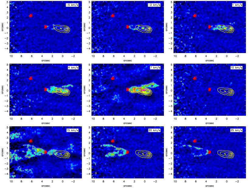
Figure 14: The ¹²CO (3-2) channel map. The central velocity is 10.3 km s^-1. The grey contours show the flux density levels of $4\sigma\times$(1, 2, 3, 4 5) with $1\sigma=2.74\times 10^{-2}$ Jy beam^-1. The 0.89 mm continuum is superposed on the map in red contours with levels of 5$\sigma\times$(1, 2, 4, 6, 10, 20) and 1$\sigma$=4.0$\times$10^-4 Jy beam^-1. The GNIRS K-band emission is overlaid onto the channel map with the yellow contours, in which the contour levels are $20\sigma$, $50\sigma$, $100\sigma$, $150\sigma$, and $200\sigma$ with 1$\sigma$=8.4 in arbitrary units. The beam size is presented in bottom left in each panel.

UTF8gbsn

References

- Antoniucci et al. (2014) Antoniucci, S., Giannini, T., Li Causi, G., & Lorenzetti, D. 2014, ApJ, 782, 51, doi: 10.1088/0004-637X/782/1/51
- Audard et al. (2014) Audard, M., Ábrahám, P., Dunham, M. M., et al. 2014, in Protostars and Planets VI, ed. H. Beuther, R. S. Klessen, C. P. Dullemond, & T. Henning, 387, doi: 10.2458/azu_uapress_9780816531240-ch017
- Bae et al. (2014) Bae, J., Hartmann, L., Zhu, Z., & Nelson, R. P. 2014, ApJ, 795, 61, doi: 10.1088/0004-637X/795/1/61
- Baek et al. (2020) Baek, G., MacFarlane, B. A., Lee, J.-E., et al. 2020, ApJ, 895, 27, doi: 10.3847/1538-4357/ab8ad4
- Balog et al. (2014) Balog, Z., Muzerolle, J., Flaherty, K., et al. 2014, ApJ, 789, L38, doi: 10.1088/2041-8205/789/2/L38
- Beck et al. (2008) Beck, T. L., McGregor, P. J., Takami, M., & Pyo, T.-S. 2008, ApJ, 676, 472, doi: 10.1086/527528
- Black & van Dishoeck (1987) Black, J. H., & van Dishoeck, E. F. 1987, ApJ, 322, 412, doi: 10.1086/165740
- Brown et al. (2013) Brown, J. M., Pontoppidan, K. M., van Dishoeck, E. F., et al. 2013, ApJ, 770, 94, doi: 10.1088/0004-637X/770/2/94
- Burns et al. (2015) Burns, R. A., Imai, H., Handa, T., et al. 2015, MNRAS, 453, 3163, doi: 10.1093/mnras/stv1836
- Burns et al. (2020) Burns, R. A., Sugiyama, K., Hirota, T., et al. 2020, Nature Astronomy, 4, 506, doi: 10.1038/s41550-019-0989-3
- Caratti o Garatti et al. (2015) Caratti o Garatti, A., Stecklum, B., Linz, H., Garcia Lopez, R., & Sanna, A. 2015, A&A, 573, A82, doi: 10.1051/0004-6361/201423992
- Caratti o Garatti et al. (2017) Caratti o Garatti, A., Stecklum, B., Garcia Lopez, R., et al. 2017, Nature Physics, 13, 276, doi: 10.1038/nphys3942
- Casali et al. (2007) Casali, M., Adamson, A., Alves de Oliveira, C., et al. 2007, A&A, 467, 777, doi: 10.1051/0004-6361:20066514
- Connelley et al. (2009) Connelley, M. S., Hodapp, K. W., & Fuller, G. A. 2009, AJ, 137, 3494, doi: 10.1088/0004-6256/137/3/3494
- Contreras Peña et al. (2020) Contreras Peña, C., Johnstone, D., Baek, G., et al. 2020, MNRAS, 495, 3614, doi: 10.1093/mnras/staa1254
- Contreras Peña et al. (2017) Contreras Peña, C., Lucas, P. W., Kurtev, R., et al. 2017, Monthly Notices of the Royal Astronomical Society, 465, 3039, doi: 10.1093/mnras/stw2802
- Cook et al. (2019) Cook, B. T., Tobin, J. J., Skrutskie, M. F., & Nelson, M. J. 2019, A&A, 626, A51, doi: 10.1051/0004-6361/201935419
- Cutri et al. (2021) Cutri, R. M., Wright, E. L., Conrow, T., et al. 2021, VizieR Online Data Catalog, II/328
- Cyganowski et al. (2008) Cyganowski, C. J., Whitney, B. A., Holden, E., et al. 2008, AJ, 136, 2391, doi: 10.1088/0004-6256/136/6/2391
- Dempsey et al. (2013) Dempsey, J. T., Friberg, P., Jenness, T., et al. 2013, MNRAS, 430, 2534, doi: 10.1093/mnras/stt090
- Dunham et al. (2015) Dunham, M. M., Allen, L. E., Evans, II, N. J., et al. 2015, ApJS, 220, 11, doi: 10.1088/0067-0049/220/1/11
- Fazio et al. (2004) Fazio, G. G., Hora, J. L., Allen, L. E., et al. 2004, ApJS, 154, 10, doi: 10.1086/422843
- Fedriani et al. (2020) Fedriani, R., Caratti o Garatti, A., Koutoulaki, M., et al. 2020, A&A, 633, A128, doi: 10.1051/0004-6361/201936748
- Fischer et al. (2019) Fischer, W. J., Safron, E., & Megeath, S. T. 2019, ApJ, 872, 183, doi: 10.3847/1538-4357/ab01dc
- Fischer et al. (2020) Fischer, W. J., Megeath, S. T., Furlan, E., et al. 2020, ApJ, 905, 119, doi: 10.3847/1538-4357/abc7cb
- Furlan et al. (2016) Furlan, E., Fischer, W. J., Ali, B., et al. 2016, The Astrophysical Journal Supplement Series, 224, 5, doi: 10.3847/0067-0049/224/1/5
- Gaia Collaboration et al. (2018) Gaia Collaboration, Brown, A. G. A., Vallenari, A., et al. 2018, A&A, 616, A1, doi: 10.1051/0004-6361/201833051
- Getman et al. (2017) Getman, K. V., Broos, P. S., Kuhn, M. A., et al. 2017, ApJS, 229, 28, doi: 10.3847/1538-4365/229/2/28
- Giannini et al. (2006) Giannini, T., McCoey, C., Nisini, B., et al. 2006, A&A, 459, 821, doi: 10.1051/0004-6361:20065127
- Giannini et al. (2002) Giannini, T., Nisini, B., Caratti o Garatti, A., & Lorenzetti, D. 2002, ApJ, 570, L33, doi: 10.1086/340883
- Gibb & Little (2000) Gibb, A. G., & Little, L. T. 2000, MNRAS, 313, 663, doi: 10.1046/j.1365-8711.2000.03235.x
- Gledhill & Forde (2012) Gledhill, T. M., & Forde, K. P. 2012, MNRAS, 421, 346, doi: 10.1111/j.1365-2966.2011.20309.x
- Green et al. (2013) Green, J. D., Evans, II, N. J., Kóspál, Á., et al. 2013, ApJ, 772, 117, doi: 10.1088/0004-637X/772/2/117
- Guo et al. (2020) Guo, Z., Lucas, P. W., Contreras Peña, C., et al. 2020, MNRAS, 492, 294, doi: 10.1093/mnras/stz3374
- Gutermuth et al. (2009) Gutermuth, R. A., Megeath, S. T., Myers, P. C., et al. 2009, ApJS, 184, 18, doi: 10.1088/0067-0049/184/1/18
- Hartmann & Kenyon (1996) Hartmann, L., & Kenyon, S. J. 1996, ARA&A, 34, 207, doi: 10.1146/annurev.astro.34.1.207
- Haschick et al. (1983) Haschick, A. D., Moran, J. M., Rodriguez, L. F., & Ho, P. T. P. 1983, ApJ, 265, 281, doi: 10.1086/160673
- Herczeg et al. (2011) Herczeg, G. J., Brown, J. M., van Dishoeck, E. F., & Pontoppidan, K. M. 2011, A&A, 533, A112, doi: 10.1051/0004-6361/201016246
- Herczeg et al. (2012) Herczeg, G. J., Karska, A., Bruderer, S., et al. 2012, A&A, 540, A84, doi: 10.1051/0004-6361/201117914
- Herczeg et al. (2017) Herczeg, G. J., Johnstone, D., Mairs, S., et al. 2017, The Astrophysical Journal, 849, 43, doi: 10.3847/1538-4357/aa8b62
- Hillenbrand et al. (2013) Hillenbrand, L. A., Miller, A. A., Covey, K. R., et al. 2013, AJ, 145, 59, doi: 10.1088/0004-6256/145/3/59
- Hillenbrand et al. (2018) Hillenbrand, L. A., Contreras Peña, C., Morrell, S., et al. 2018, ApJ, 869, 146, doi: 10.3847/1538-4357/aaf414
- Hirota et al. (2021) Hirota, T., Cesaroni, R., Moscadelli, L., et al. 2021, A&A, 647, A23, doi: 10.1051/0004-6361/202039798
- Holland et al. (2013) Holland, W. S., Bintley, D., Chapin, E. L., et al. 2013, Monthly Notices of the Royal Astronomical Society, 430, 2513, doi: 10.1093/mnras/sts612
- Hsieh et al. (2019) Hsieh, T.-H., Murillo, N. M., Belloche, A., et al. 2019, ApJ, 884, 149, doi: 10.3847/1538-4357/ab425a
- Ilee et al. (2013) Ilee, J. D., Wheelwright, H. E., Oudmaijer, R. D., et al. 2013, MNRAS, 429, 2960, doi: 10.1093/mnras/sts537
- Johnstone et al. (2001) Johnstone, D., Fich, M., Mitchell, G. F., & Moriarty-Schieven, G. 2001, ApJ, 559, 307, doi: 10.1086/322323
- Johnstone et al. (2013) Johnstone, D., Hendricks, B., Herczeg, G. J., & Bruderer, S. 2013, ApJ, 765, 133, doi: 10.1088/0004-637X/765/2/133
- Johnstone et al. (2018) Johnstone, D., Herczeg, G. J., Mairs, S., et al. 2018, The Astrophysical Journal, 854, 31, doi: 10.3847/1538-4357/aaa764
- Jørgensen et al. (2015) Jørgensen, J. K., Visser, R., Williams, J. P., & Bergin, E. A. 2015, A&A, 579, A23, doi: 10.1051/0004-6361/201425317
- Kang et al. (2015) Kang, M., Choi, M., Stutz, A. M., & Tatematsu, K. 2015, ApJ, 814, 31, doi: 10.1088/0004-637X/814/1/31
- Karska et al. (2018) Karska, A., Kaufman, M. J., Kristensen, L. E., et al. 2018, ApJS, 235, 30, doi: 10.3847/1538-4365/aaaec5
- Kirk et al. (2016) Kirk, H., Di Francesco, J., Johnstone, D., et al. 2016, ApJ, 817, 167, doi: 10.3847/0004-637X/817/2/167
- Kóspál et al. (2007) Kóspál, Á., Ábrahám, P., Prusti, T., et al. 2007, A&A, 470, 211, doi: 10.1051/0004-6361:20066108
- Kóspál et al. (2017) Kóspál, Á., Ábrahám, P., Westhues, C., & Haas, M. 2017, A&A, 597, L10, doi: 10.1051/0004-6361/201629447
- Kóspál et al. (2020) Kóspál, Á., Szabó, Z. M., Ábrahám, P., et al. 2020, ApJ, 889, 148, doi: 10.3847/1538-4357/ab6174
- Kounkel et al. (2018) Kounkel, M., Covey, K., Suárez, G., et al. 2018, AJ, 156, 84, doi: 10.3847/1538-3881/aad1f1
- Laos et al. (2021) Laos, S., Greene, T. P., Najita, J. R., & Stassun, K. G. 2021, ApJ, 921, 110, doi: 10.3847/1538-4357/ac1f1b
- Lee (2007) Lee, J.-E. 2007, Journal of Korean Astronomical Society, 40, 83, doi: 10.5303/JKAS.2007.40.4.083
- Lee et al. (2010) Lee, J.-E., Lee, H.-G., Shinn, J.-H., et al. 2010, ApJ, 709, L74, doi: 10.1088/2041-8205/709/1/L74
- Lee et al. (2016) Lee, S., Lee, J.-E., Park, S., et al. 2016, ApJ, 826, 179, doi: 10.3847/0004-637X/826/2/179
- Lee et al. (2020) Lee, Y.-H., Johnstone, D., Lee, J.-E., et al. 2020, ApJ, 903, 5, doi: 10.3847/1538-4357/abb6fe
- Lee et al. (2021) —. 2021, arXiv e-prints, arXiv:2107.10750. https://arxiv.org/abs/2107.10750
- Lucas et al. (2017) Lucas, P. W., Smith, L. C., Contreras Peña, C., et al. 2017, MNRAS, 472, 2990, doi: 10.1093/mnras/stx2058
- MacFarlane et al. (2019a) MacFarlane, B., Stamatellos, D., Johnstone, D., et al. 2019a, MNRAS, 487, 5106, doi: 10.1093/mnras/stz1512
- MacFarlane et al. (2019b) —. 2019b, MNRAS, 1508, doi: 10.1093/mnras/stz1570
- Mainzer et al. (2011) Mainzer, A., Bauer, J., Grav, T., et al. 2011, ApJ, 731, 53, doi: 10.1088/0004-637X/731/1/53
- Mainzer et al. (2014) Mainzer, A., Bauer, J., Cutri, R. M., et al. 2014, ApJ, 792, 30, doi: 10.1088/0004-637X/792/1/30
- Mairs et al. (2017a) Mairs, S., Johnstone, D., Kirk, H., et al. 2017a, The Astrophysical Journal, 849, 107, doi: 10.3847/1538-4357/aa9225
- Mairs et al. (2017b) Mairs, S., Lane, J., Johnstone, D., et al. 2017b, The Astrophysical Journal, 843, 55, doi: 10.3847/1538-4357/aa7844
- Mairs et al. (2021) Mairs, S., Dempsey, J. T., Bell, G. S., et al. 2021, arXiv e-prints, arXiv:2107.13558. https://arxiv.org/abs/2107.13558
- Maíz Apellániz et al. (2020) Maíz Apellániz, J., Pantaleoni González, M., Barbá, R. H., García-Lario, P., & Nogueras-Lara, F. 2020, MNRAS, 496, 4951, doi: 10.1093/mnras/staa1790
- Manoj et al. (2013) Manoj, P., Watson, D. M., Neufeld, D. A., et al. 2013, ApJ, 763, 83, doi: 10.1088/0004-637X/763/2/83
- Manoj et al. (2016) Manoj, P., Green, J. D., Megeath, S. T., et al. 2016, ApJ, 831, 69, doi: 10.3847/0004-637X/831/1/69
- McMahon et al. (2013) McMahon, R. G., Banerji, M., Gonzalez, E., et al. 2013, The Messenger, 154, 35
- McMullin et al. (2007) McMullin, J. P., Waters, B., Schiebel, D., Young, W., & Golap, K. 2007, in Astronomical Society of the Pacific Conference Series, Vol. 376, Astronomical Data Analysis Software and Systems XVI, ed. R. A. Shaw, F. Hill, & D. J. Bell, 127
- Megeath et al. (2012) Megeath, S. T., Gutermuth, R., Muzerolle, J., et al. 2012, AJ, 144, 192, doi: 10.1088/0004-6256/144/6/192
- Mitchell et al. (2001) Mitchell, G. F., Johnstone, D., Moriarty-Schieven, G., Fich, M., & Tothill, N. F. H. 2001, ApJ, 556, 215, doi: 10.1086/321574
- Motte et al. (2001) Motte, F., André, P., Ward-Thompson, D., & Bontemps, S. 2001, A&A, 372, L41, doi: 10.1051/0004-6361:20010543
- Muzerolle et al. (2013) Muzerolle, J., Furlan, E., Flaherty, K., Balog, Z., & Gutermuth, R. 2013, Nature, 493, 378, doi: 10.1038/nature11746
- Nagy et al. (2020) Nagy, Z., Menechella, A., Megeath, S. T., et al. 2020, A&A, 642, A137, doi: 10.1051/0004-6361/201937342
- Najita et al. (1996) Najita, J., Carr, J. S., Glassgold, A. E., Shu, F. H., & Tokunaga, A. T. 1996, ApJ, 462, 919, doi: 10.1086/177205
- Nomura et al. (2007) Nomura, H., Aikawa, Y., Tsujimoto, M., Nakagawa, Y., & Millar, T. J. 2007, ApJ, 661, 334, doi: 10.1086/513419
- Oh et al. (2018) Oh, H., Pyo, T.-S., Koo, B.-C., et al. 2018, ApJ, 858, 23, doi: 10.3847/1538-4357/aabba4
- Okoda et al. (2021) Okoda, Y., Oya, Y., Francis, L., et al. 2021, ApJ, 910, 11, doi: 10.3847/1538-4357/abddb1
- Park et al. (2021) Park, W., Lee, J.-E., Contreras Peña, C., et al. 2021, arXiv e-prints, arXiv:2107.10751. https://arxiv.org/abs/2107.10751
- Phillips et al. (2001) Phillips, R. R., Gibb, A. G., & Little, L. T. 2001, MNRAS, 326, 927, doi: 10.1046/j.1365-8711.2001.04502.x
- Pilbratt et al. (2010) Pilbratt, G. L., Riedinger, J. R., Passvogel, T., et al. 2010, A&A, 518, L1, doi: 10.1051/0004-6361/201014759
- Plunkett et al. (2015) Plunkett, A. L., Arce, H. G., Mardones, D., et al. 2015, Nature, 527, 70, doi: 10.1038/nature15702
- Rebull et al. (2014) Rebull, L. M., Cody, A. M., Covey, K. R., et al. 2014, AJ, 148, 92, doi: 10.1088/0004-6256/148/5/92
- Reipurth (1989) Reipurth, B. 1989, Nature, 340, 42, doi: 10.1038/340042a0
- Safron et al. (2015) Safron, E. J., Fischer, W. J., Megeath, S. T., et al. 2015, ApJ, 800, L5, doi: 10.1088/2041-8205/800/1/L5
- Scholz et al. (2013) Scholz, A., Froebrich, D., & Wood, K. 2013, MNRAS, 430, 2910, doi: 10.1093/mnras/stt091
- Smith (1995) Smith, M. D. 1995, A&A, 296, 789
- Spezzi et al. (2015) Spezzi, L., Petr-Gotzens, M. G., Alcalá, J. M., et al. 2015, A&A, 581, A140, doi: 10.1051/0004-6361/201425417
- Stecklum et al. (2021) Stecklum, B., Wolf, V., Linz, H., et al. 2021, A&A, 646, A161, doi: 10.1051/0004-6361/202039645
- Stutz et al. (2013) Stutz, A. M., Tobin, J. J., Stanke, T., et al. 2013, The Astrophysical Journal, 767, 36, doi: 10.1088/0004-637X/767/1/36
- Szegedi-Elek et al. (2020) Szegedi-Elek, E., Ábrahám, P., Wyrzykowski, Ł., et al. 2020, ApJ, 899, 130, doi: 10.3847/1538-4357/aba129
- Takami et al. (2006) Takami, M., Chrysostomou, A., Ray, T. P., et al. 2006, ApJ, 641, 357, doi: 10.1086/500352
- Tappe et al. (2012) Tappe, A., Forbrich, J., Martín, S., Yuan, Y., & Lada, C. J. 2012, ApJ, 751, 9, doi: 10.1088/0004-637X/751/1/9
- Tobin et al. (2015) Tobin, J. J., Stutz, A. M., Megeath, S. T., et al. 2015, ApJ, 798, 128, doi: 10.1088/0004-637X/798/2/128
- Tobin et al. (2016) Tobin, J. J., Stutz, A. M., Manoj, P., et al. 2016, ApJ, 831, 36, doi: 10.3847/0004-637X/831/1/36
- Tobin et al. (2020a) Tobin, J. J., Sheehan, P. D., Reynolds, N., et al. 2020a, ApJ, 905, 162, doi: 10.3847/1538-4357/abc5bf
- Tobin et al. (2020b) Tobin, J. J., Sheehan, P. D., Megeath, S. T., et al. 2020b, ApJ, 890, 130, doi: 10.3847/1538-4357/ab6f64
- Tychoniec et al. (2019) Tychoniec, Ł., Hull, C. L. H., Kristensen, L. E., et al. 2019, A&A, 632, A101, doi: 10.1051/0004-6361/201935409
- Varricatt et al. (2010) Varricatt, W. P., Davis, C. J., Ramsay, S., & Todd, S. P. 2010, MNRAS, 404, 661, doi: 10.1111/j.1365-2966.2010.16356.x
- Visser et al. (2012) Visser, R., Kristensen, L. E., Bruderer, S., et al. 2012, A&A, 537, A55, doi: 10.1051/0004-6361/201117109
- Wang & Chen (2019) Wang, S., & Chen, X. 2019, ApJ, 877, 116, doi: 10.3847/1538-4357/ab1c61
- Weingartner & Draine (2001) Weingartner, J. C., & Draine, B. T. 2001, ApJ, 548, 296, doi: 10.1086/318651
- Wright et al. (2010) Wright, E. L., Eisenhardt, P. R. M., Mainzer, A. K., et al. 2010, AJ, 140, 1868, doi: 10.1088/0004-6256/140/6/1868
- Zakri et al. (2022) Zakri, W., Megeath, S. T., Fischer, W. J., et al. 2022, arXiv e-prints, arXiv:2201.04647. https://arxiv.org/abs/2201.04647
- Zhu et al. (2007) Zhu, Z., Hartmann, L., Calvet, N., et al. 2007, ApJ, 669, 483, doi: 10.1086/521345