$\theta$ dependence of $T_{c}$ in 4d SU(3) Yang-Mills theory with histogram method and the Lee-Yang zeros in the large $N$ limit

Abstract

The phase diagram on the $\theta$-$T$ plane in four dimensional SU(3) Yang-Mills theory is explored. We revisit the $\theta$ dependence of the deconfinement transition temperature, $T_{c}(\theta)$, on the lattice through the constraint effective potential for Polyakov loop. The $\theta$ term is introduced by the reweighting method, and the critical $\beta$ is determined to $\theta\sim 0.75$, where the interpolation in $\beta$ is carried out by the multipoint reweighting method. The $\theta$ dependence of $T_{c}$ obtained here turns out to be consistent with the previous result by D’Elia and Negro DElia:2012pvq ; DElia:2013uaf . We also derive $T_{c}(\theta)$ by classifying configurations into the high and low temperature phases and applying the Clausius-Clapeyron equation. It is found that the potential barrier in the double well potential at $T_{c}(\theta)$ becomes higher with $\theta$, which suggests that the first order transition continues robustly above $\theta\sim 0.75$. Using information obtained here, we try to depict the expected $\theta$ dependence of the free energy density at $T\mathrel{\hbox to0.0pt{\raise 2.20013pt\hbox{$<$}\hss}{\lower 2.20013pt\hbox{$\sim$}}}T_{c}(0)$, which crosses the first order transition line at an intermediate value of $\theta$. Finally, how the Lee-Yang zeros associated with the spontaneous CP violation appear is discussed formally in the large $N$ limit, and the locations of them are found to be $(\theta_{R},\theta_{I})=\left((2m+1)\pi,\frac{2n+1}{2\chi V_{4}}\right)$ with $m$ and $n$ arbitrary integers.

1 Introduction

To understand phases realized in a theory and how those change under varying parameters is one of the most attractive aspects of field theory. In this work, we consider the $\theta$-$T$ phase diagram for four dimensional SU(3) Yang-Mills theory, where $\theta$ is a parameter controlling relative weights of different topological sectors in the path integral Callan:1976je and $T$ denotes temperature.

In the high temperature deconfined phase, it has been known that instanton calculus Polyakov:1975rs ; Belavin:1975fg ; Harrington:1978ve is reliable Gross:1980br ; Frison:2016vuc , and no phase transition is expected to occur by changing $\theta$. Interestingly, in the low temperature phase, it has been argued that spontaneous CP violation takes place at $\theta=\pi$ if the vacuum is in the confined phase there Gaiotto:2017yup ; Kitano:2017jng . In the large $N$ limit, the occurrence of the CP violation at $\theta=\pi$ seemed to be established tHooft:1973alw ; Witten:1980sp ; tHooft:1981bkw ; Witten:1998uka . It is speculated based on numerical evidences that CP symmetry is also broken at $\theta=\pi$ in the opposite limit, i.e. SU(2) Yang-Mills theory Kitano:2020mfk . Recently, the $\theta$ dependence of the vacuum energy density of SU(2) theory was calculated on the lattice for $\theta\mathrel{\hbox to0.0pt{\raise 2.20013pt\hbox{$<$}\hss}{\lower 2.20013pt\hbox{$\sim$}}}3\pi/2$, and the spontaneous CP violation at $\theta=\pi$ is concluded in Kitano:2021jho , where a newly developed method, called the subvolume method, is applied.

Although it is straightforward to apply the subvolume method to explore the phase diagram of SU(3) Yang-Mills theory, it requires some cares. Since the subvolume method can be seen as a variant of the reweighting method, it may suffer from the so-called overlap problem. In the SU(3) case, the deconfinement transition is of first order, and when used to study phases with varying $\theta$ the method may fail to detect the phase transition and follow the original branch even after passing the transition point .

One approach complementary to calculating the free energy density with the subvolume method is to identify the curve of $T_{c}(\theta)$ in the phase diagram. Especially, if one could have succeeded to determine $T_{c}(\theta)$ to $\theta=\pi$, it becomes clear whether $T_{c}(\theta)$ touches to the $T=0$ axis or not. Unfortunately, it is difficult to estimate the critical temperature at general values of $\theta$ because the standard lattice techniques do not work in the region with $\theta\mathrel{\hbox to0.0pt{\raise 2.20013pt\hbox{$>$}\hss}{\lower 2.20013pt\hbox{$\sim$}}}O(1)$, and hence as a first step we constrain our discussion to the small $\theta$ region, where several numerical techniques are available. In DElia:2012pvq ; DElia:2013uaf , $T_{c}(\theta)$ is determined in such a region with the analytic continuation from imaginary $\theta$ and the reweighting method by monitoring the Polyakov loop susceptibility and found to decrease with $\theta$. The aims of this work are to confirm this $\theta$ dependence and obtain different insights through a different approach.

In this work, we construct the constraint effective potential ORaifeartaigh:1986axd from the histogram of the Polyakov loop to identify $T_{c}(\theta)$. The $\theta$ term is introduced by the standard reweighting technique. With the effective potential at hand, we hope to gain some insights on how the potential shape changes or whether the first order transition at $T_{c}(\theta)$ becomes stronger or weaker with $\theta$. Furthermore, according to the resulting histogram it becomes possible to classify each configuration into the high and low temperature phases. Using those configurations, we can separately calculate the free energy density in two phases and combine them to depict the $\theta$ dependence of the free energy density across the first order phase transition.

In the discussion of the phase transition, the zeros of partition function Yang:1952be ; Lee:1952ig ; Fischer:1965rna are often analyzed. On the $\theta$-$T$ plane, at least, two kinds of phase transitions exist corresponding to the center and CP symmetry breaking, respectively. After briefly recalling how the zeros appear in the deconfinement transition, we perform a formal discussion to explore the locations of them associated with the spontaneous CP violation at $\theta=\pi$ in the large $N$ limit.

In sec. 2, we briefly describe the lattice setup and the methods as well as some basic results to show the features of the ensembles used in the following analysis. In sec. 3, the details of the numerical analysis and the results for $T_{c}(\theta)$ are presented, where the consistencies with the previous result and the Clausius-Clapeyron equation are tested. The analyses using the configurations separated into high and low temperature phases are also given here. In sec. 4, the Lee-Yang zeros associated with phase transitions relevant to the present study are explored. Finally, the summary and the outlook are stated in sec. 5. In Appendix A, the application of the Clapeyron-Clausius equation to the determination of $dT(\theta)/d\theta\big{|}_{\theta=0}$ is described.

2 Lattice Setup and method

2.1 parameters

The partition function for lattice SU($N$) Yang-Mills theory including the $\theta$ term is

$$Z(\beta,\theta)=\int\!{\cal D}U\,e^{-6\,\beta\,N_{\rm site}\,\hat{s}_{g}-i\theta\hat{Q}}\ ,\qquad$$ (1)

where $\hat{s}_{g}$ is the action density averaged over the number of the lattice sites, $N_{\rm site}$, and given by the sum of the average of the plaquette $\hat{w}_{P}$ and the rectangle $\hat{w}_{R}$,

$$\hat{s}_{g}= \ c_{0}(1-\hat{w}_{P})+2\,c_{1}(1-\hat{w}_{R})\ ,$$ (2)

where $c_{0}$ and $c_{1}$ satisfying $c_{0}=1-8c_{1}$ are the improvement coefficients for the lattice gauge action and $c_{1}=-0.331$ is taken corresponding to the Iwasaki RG improved action Iwasaki:1985we . The lattice gauge coupling is tuned by changing $\beta=2N/g^{2}$. Throughout the paper, a hat $\ \hat{}\$ is attached to functions of link variable, e.g. $\hat{s}_{g}=\hat{s}_{g}[U]$, to distinguish from $c$-numbers without a hat $\ \hat{}\$.

In the definition of the topological charge on the lattice $\hat{Q}=\sum_{x}\hat{q}(x)$, we employ the five-loop improved topological charge density operator $\hat{q}(x)$ deForcrand:1997esx . The topological charge for a given configuration is calculated after $n_{\rm APE}$ times of the APE smearing Albanese:1987ds , and observables are extrapolated to $n_{\rm APE}=0$ using those obtained in the range of $n_{\rm APE}=[35,55]$, which is chosen following the criterion given in Kitano:2020mfk . Since the $n_{\rm APE}$ dependence for any observables studied here turns out to be negligibly small, we will present results without specifying $n_{\rm APE}$.

The number of lattice sites is $N_{\rm site}=N_{S}^{3}\times N_{T}$ with $N_{S}=24$ and $N_{T}=6$. We choose four values of $\beta$ with $N=3$ to cover the critical $\beta$ at $\theta=0$, $\beta_{c}\sim 2.515$ Okamoto:1999hi . The number of configurations at each $\beta$ is 40,000. The statistical errors are estimated by the jackknife method. Simulation parameters, $T/T_{c}$ and the statistics are summarized in Tab. 1.

	$\beta$	$T/T_{c}$	statistics
SU(3)	2.505	0.984	40,000
Iwasaki RG	2.510	0.992	40,000
$24^{3}\times 6$	2.515	1.000	40,000
	2.520	1.008	40,000

Table 1: The lattice parameters of the ensembles and other informations.

2.2 constraint effective potential

The histogram method or the constraint effective potential described below is a useful tool especially when exploring phase boundaries and has been used, for example, in the study of the phase diagram for many flavor QCD Ejiri:2012rr or in searching for the critical end point in the heavy quark region Ejiri:2019csa .

The histogram for CP even operators $\hat{o}_{i}$ ($i=1,2,\cdots,N_{o}$) measured at $\beta$ and $\theta$ is defined by

$$p(o_{1},\cdots,o_{N_{o}};\beta,\theta) =\ \frac{1}{Z(\beta,\theta)}\int\!\!{\cal D}U\left\{\displaystyle\prod_{i=1}^{N_{o}}\delta(\hat{o}_{i}-o_{i})\right\}e^{-6\beta N_{\rm site}s_{g}-i\theta\hat{Q}}$$

$$=\ {\left\langle\,\left\{\displaystyle\prod_{i=1}^{N_{o}}\delta(\hat{o}_{i}-o_{i})\right\}\cos(\theta\hat{Q})\,\right\rangle_{\beta}\over\left\langle\,\cos(\theta\hat{Q})\,\right\rangle_{\beta}}\ ,$$ (3)

$$p(o_{2},\cdots,o_{N_{o}};\beta,\theta) =\ \int\!\!do_{1}\,p(o_{1},\cdots,o_{N_{o}};\beta,\theta)\ ,$$ (4)

where $o_{i}$ denotes a c-number. As indicated in (3), the $\theta$ term is interpreted as a part of observable, that is, introduced through the reweighting method. $\left\langle\,\cdots\,\right\rangle_{\beta}$ denotes the expectation value over the configurations generated at $\beta$ without the $\theta$ term.

Some examples are shown in what follows because they would help to grab the features of ensembles used in this work. The first examples with $N_{o}=1$ shown in Fig. 1 are the histograms for the action density, $p(s_{g};\beta,0)$, and the modulus of the Polyakov loop, $p(\omega;\beta,0)$ at $\theta=0$, where

$$\hat{\omega}=\left|\hat{\Omega}\right|=\left|\frac{1}{N_{S}^{3}\,N_{c}}\sum_{\vec{x}}{\rm Tr_{c}}\big{[}\displaystyle\prod_{t=1}^{N_{T}}U_{4}(\vec{x},t)\big{]}\right|\ ,$$ (5)

where $U_{4}(\vec{x},t)$ is the link variable in time direction. $\hat{\omega}$ is an approximate order parameter for the confinement-deconfinement transition.

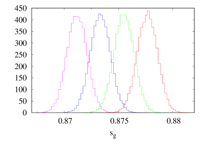
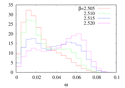
Figure 1: The histogram of the action $s_{g}$ (left) and the modulus of the Polyakov loop $\omega$ (right) for the four ensembles.

In each plot, the four histograms correspond to the four values of $\beta$. Each histogram for $s_{g}$ well overlaps with, at least, one of others, which becomes important later when interpolating histograms in $\beta$. Some of the histograms for $\omega$ show a clear double-peak, which indicates that the $\beta$ value for those are close to the critical point.

Figure 2 shows examples with $N_{o}=2$, the histogram of the real and imaginary part of the Polyakov loop at $\theta=0$, $p({\rm Re}\,\Omega,{\rm Im}\,\Omega;\beta,0)$, where it is seen that the center symmetry is gradually broken with $\beta$.

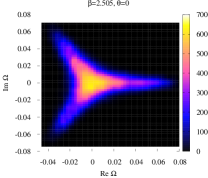
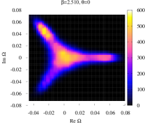
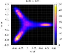
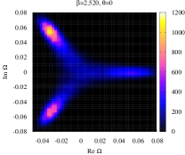
Figure 2: Two dimensional histogram on the ${\rm Re}\,\Omega$-${\rm Im}\,\Omega$ plane. The results at $\beta=2.505$, 2.510, 2.515 and 2.520 are shown from left to right.

Another example with $N_{o}=2$ shown in Fig 3 is the histogram for $s_{g}$ and $\omega$, $p(s_{g},\omega;\beta,\theta)$, at $\theta=0$ and $2\pi/10$. These histograms are used in the following analyses and the intervals of histogram are set to 0.0005 for $s_{g}$ and 0.005 for $\omega$. One or two peaks are observed around $\omega\sim 0.01$ and/or $0.05$, where the former gets lower and the latter higher with $\theta$. In the plot for $\theta=0$ and $\beta=2.515$, the two peaks are located at almost the same value of $s_{g}$ and hence it would be difficult to identify $\beta_{c}$ only by looking at the histogram for $s_{g}$, which is contrary to the case using the Wilson plaquette gauge action Saito:2013vja .

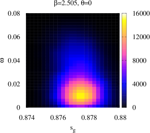
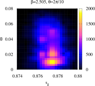
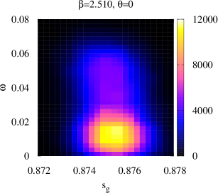
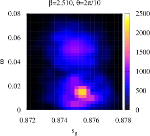
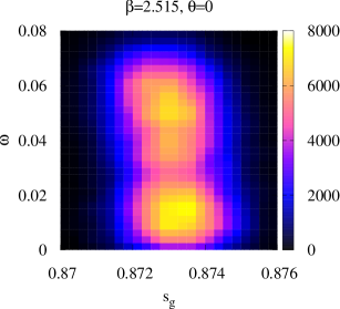
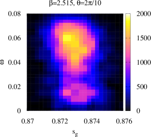
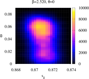
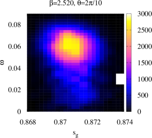
Figure 3: Two dimensional histogram on the $s_{g}$-$\omega$ plane at $\beta=2.505$ 2.510, 2.515, 2.520 from top to bottom.

Using a histogram like above, we can define the constraint effective potential by

$$V_{\rm eff}(o_{1},\cdots,o_{N_{o}};\beta,\theta)=-\frac{1}{N_{\rm site}}\ln p(o_{1},\cdots,o_{N_{o}};\beta,\theta)\ ,$$ (6)

which coincides with the ordinary effective potential in the infinite volume limit ORaifeartaigh:1986axd . We investigate the constraint effective potential for $\hat{\omega}$,

$$V_{\rm eff}(\omega;\beta,\theta) =-\frac{1}{N_{\rm site}}\ln p(\omega;\beta,\theta)\ .$$ (7)

We can immediately calculate $V_{\rm eff}(\omega;\beta,\theta)$ by using the histograms at four values of $\beta$ following (3). To show $V_{\rm eff}(\omega;\beta,\theta)$, we separate it into the $\theta=0$ contribution and the correction to that due to non-zero $\theta$ defined by

$$\delta V_{\rm eff}(\omega;\beta,\theta)= V_{\rm eff}(\omega;\beta,\theta)-V_{\rm eff}(\omega;\beta,0)=\ -\frac{1}{N_{\rm site}}\ln{p(\omega;\beta,\theta)\over p(\omega;\beta,0)}\ .$$ (8)

$V_{\rm eff}$ and $\delta V_{\rm eff}$ are shown in Fig. 4.

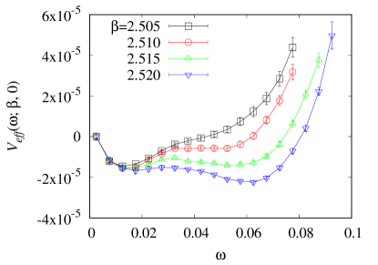
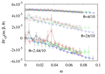
Figure 4: $V_{\mathrm{eff}}(\omega;\beta,0)$ (left) obtained at four $\beta$ values and $\delta V_{\mathrm{eff}}(\omega;\beta,\theta)$ (right) for four $\beta$ and three different $\theta$. In both plots, the same symbols are used and the data are shifted in the vertical direction for visibility.

It is seen that at $\theta=0$ the global minimum transitions around $\beta=2.515$. The contribution of the nonzero $\theta$ to the potential turns out to depend on $\theta$ but not on $\beta$ strongly. It is also found that the nonzero $\theta$ contributions are approximately linear in $\omega$ with a negative slope being steeper with $\theta$. These observations immediately tell us that $\beta_{c}$ decreases with $\theta$.

In order to explore the origin of the negative slope, we examine the $Q$-$\omega$ histogram at $\theta=0$, $p(Q,\omega;\beta,0)$, shown in Fig. 5.

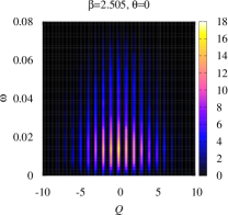
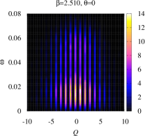
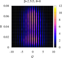
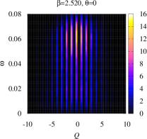
Figure 5: Two dimensional histograms on the $Q$-$\omega$ plane at four values of $\beta$.

Roughly speaking, the histogram consists of two lumps located at $\omega\sim 0.01$ and $\omega\sim 0.05$. Importantly, the former spreads in the $Q$ direction more than the later. Noticing that, up to a normalization,

$$p(\omega;\beta,\theta) =\sum_{Q}p(Q,\omega;\beta,\theta)\sim\sum_{Q}\cos(\theta Q)p(Q,\omega;\beta,0)\ ,$$ (9)

the different distribution in $Q$ yields due to the cosine factor the different suppression in $p(Q,\omega;\beta,\theta)$ and then $p(\omega;\beta,\theta)$. Since $p(Q,0.01;\beta,0)$ distributes wider in $Q$ than $p(Q,0.05;\beta,0)$, $p(0.01;\beta,\theta)$ is more suppressed. It means that the local minimum in the potential around $\omega=0.01$ becomes relatively shallower compared with the one around $\omega=0.05$ when $\theta$ increases from 0. Therefore, the reason for the negative slope is attributed to the different distribution of $Q$ in $p(Q,\omega;\beta,0)$ in a large and small $\omega$ region. The distribution of $Q$ is measured by the topological susceptibility, $\chi=\langle\hat{Q}^{2}\rangle_{\beta}/V$. The relationship between the negative slope and the topological susceptibilities in the low and high temperature phase becomes clear when discussing the Clapeyron-Clausius equation later.

2.3 interpolation in $\beta$

We define $\beta_{c}$ by the value of $\beta$, at which two local minima in the constraint effective potential degenerate. As inferred from Fig. 4, $\beta_{c}$ varies with $\theta$. To determine $\beta_{c}$ at arbitrary $\theta$ as precisely as possible, we apply the multipoint reweighting method Ferrenberg:1989ui ; Iwami:2015eba to the histograms for $\hat{\omega}$, allowing us to interpolate them to desired values of $\beta$.

The details on how to interpolate the histogram in $\beta$ are described below. Recalling the reweighting technique, the histogram for $\hat{s}_{g}$ and $\hat{\omega}$ at $\beta$ and $\theta$ can be written in terms of the expectation values evaluated at $\beta_{i}$ and $\theta=0$ as

$$p(s_{g},\omega;\beta,\theta)= {1\over Z(\beta,\theta)}\int{\cal D}U\,\delta(\hat{s}_{g}-s_{g})\delta(\hat{\omega}-\omega)\,e^{-6\beta N_{\rm site}\hat{s}_{g}-i\theta\hat{Q}}$$

$$= {\left\langle\,\delta(\hat{s}_{g}-s_{g})\delta(\hat{\omega}-\omega)\cos(\theta\hat{Q})\,\right\rangle_{\beta_{i}}\over\left\langle\,e^{-6(\beta-\beta_{i})N_{\rm site}(\hat{s}_{g}-s_{g})}\cos(\theta\hat{Q})\,\right\rangle_{\beta_{i}}}\ ,$$ (10)

where the numerator is given by (3). By integrating (10) over $s_{g}$, one can obtain $p(\omega;\beta,\theta)$. If there are more than one ensembles with different $\beta_{i}$’s, one can calculate (10) on each of those ensembles and take an average over them with suitable weights to determine the histogram at $\beta$.

The simplest way of making the average would be

$$p(\omega;\beta,\theta)=\ {1\over\left(\sum_{i}W_{i}\right)}\sum_{i}W_{i}\,\int\!\!ds_{g}\,{\left\langle\,\delta(\hat{s}_{g}-s_{g})\delta(\hat{\omega}-\omega)\cos(\theta\hat{Q})\,\right\rangle_{\beta_{i}}\over\left\langle\,e^{-6(\beta-\beta_{i})N_{\rm site}(\hat{s}_{g}-s_{g})}\cos(\theta\hat{Q})\,\right\rangle_{\beta_{i}}}\ ,$$ (11)

with arbitrary weight $W_{i}$. Following Saito:2013vja , as an alternative, we also calculate the average by

$$p(\omega;\beta,\theta)= \ \int\!\!ds_{g}\,{\sum_{i}W_{i}\,\left\langle\,\delta(\hat{s}_{g}-s_{g})\delta(\hat{\omega}-\omega)\cos(\theta\hat{Q})\,\right\rangle_{\beta_{i}}\over\sum_{i}W_{i}\left\langle\,e^{-6(\beta-\beta_{i})N_{\rm site}(\hat{s}_{g}-s_{g})}\cos(\theta\hat{Q})\,\right\rangle_{\beta_{i}}}\ ,$$ (12)

which is obtained by rewriting (10) as

$$\left\langle\,e^{-6(\beta-\beta_{i})N_{\rm site}(\hat{s}_{g}-s_{g})}\cos(\theta\hat{Q})\,\,\right\rangle_{\beta_{i}}p(s_{g},\omega;\beta,\theta)= \ \left\langle\,\delta(\hat{s}_{g}-s_{g})\delta(\hat{\omega}-\omega)\cos(\theta\hat{Q})\,\right\rangle_{\beta_{i}}\ ,$$ (13)

and summing both sides over $i$ with a weight $W_{i}$. We examined the above averages with two different weight factors

$$W_{i}= N(\beta_{i})\ ,$$ (14)

$$W_{i}= N(\beta_{i})\times\exp\{-(\beta-\beta_{i})^{2}/\sigma_{\beta}^{2}\}\ ,$$ (15)

where $N(\beta_{i})$ is the number of configurations generated at $\beta_{i}$. $\sigma_{\beta}$ essentially sets the effective range of $\beta_{i}$ to be included in the average and is chosen to be $0.0025$ from the width of the distribution of $s_{g}$ (the left panel of Fig. 1).

It turns out that the combination of (11) and (14) is the noisiest among all and the others are qualitatively similar. In the following, we representatively show results with (12) and (14) as it does not contain tunable parameters.

Fig. 6 shows the numerator of the integrand in (12), which is the simple sum of the histogram obtained at four ensembles with the weight (14).

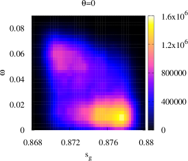
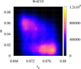
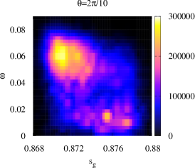
Figure 6: The numerator of the integrand in (12) for $\theta=0$, $\pi/10$ and $2\pi/10$ from left to right.

The denominator does not depend on $\omega$ and is the function of $s_{g}$, $\beta$ and $\theta$, some examples of which are shown in Fig. 7.

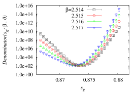
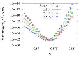
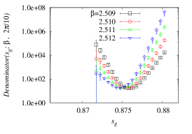
Figure 7: Some examples of the denominator of the integrand in (12) for $\theta=0$, $\pi/10$ and $2\pi/10$ from left to right. In the plot for $\theta=2\pi/10$, the results below $s_{g}\sim 0.872$ are not shown because of too large statistical uncertainties.

As seen from the figure, the denominator takes a minimum at a certain value of $s_{g}$, which depends on $\beta$. Thus, around such $s_{g}$, the integrand in (12) is relatively enhanced. Eventually, combining the numerator and denominator derives $p(s_{g},\omega;\beta,\theta)$, some examples of which are shown in Fig. 8.

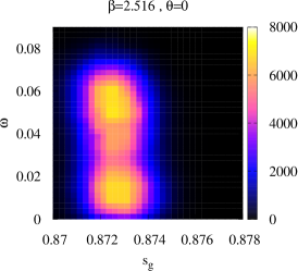
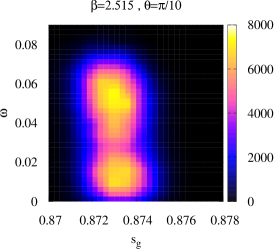
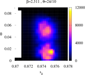
Figure 8: Examples of the resulting 2-d histogram, $p(s_{g},\omega;\beta,\theta)$, for $\theta=0$, $\pi/10$ and $2\pi/10$ from left to right.

$\beta$ in (12) is arbitrary in principle, however the interpolation does not always work in practice. For example, if only a few configurations contribute to the enhanced region of the histogram, the statistical error of that region becomes large. This necessarily happens if $\beta$ is not covered by the range of $\beta_{i}$. It is thus important to choose $\beta_{i}$’s over a suitable range and with a small enough interval. In this work, the interval of $\beta_{i}$ is chosen to be 0.005 such that the distribution of $s_{g}$ at one of the ensembles well overlaps with that at the neighboring $\beta_{i}$.

3 Numerical results

3.1 $\theta$ dependence of $T_{c}$

Integrating $p(s_{g},\omega;\beta,\theta)$ over $s_{g}$ and following (7), the constraint effective potential for $\hat{\omega}$ is obtained. Since for $\theta>\pi/4$ the results are very noisy and $\beta_{c}(\theta)$ appears to take the value out of the $\beta_{i}$ range, in the following we restrict our analysis to $\theta$ smaller than $\pi/4$.

Figure 9 shows the potential at $\theta=0$ and $2\pi/10$, where the potential value at one of the minima around $\omega\sim 0.01$ is fixed to zero.

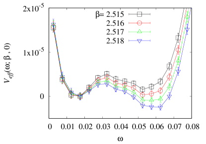
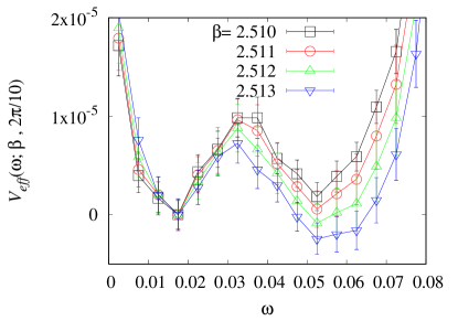
Figure 9: $V_{\rm eff}(\omega;\beta,\theta)$ at $\theta=0$ (left) and $2\pi/10$ (right).

It is seen from Fig. 9 that the potential barrier between two minima becomes higher with $\theta$ in the lattice unit, which suggests that the first order phase transition continues to be robust beyond $\theta\sim\pi/5$.

In addition to the robustness, we have also tried to see the $\theta$ dependence of the strength by calculating the latent heat. It looks consistent with constant, but the sizable statistical errors prohibits us from leading definite conclusions.

We determine $\beta_{c}$ at each $\theta$ by identifying the $\beta$ value at which the difference between two minima vanishes.

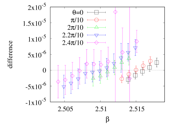
Figure 10: The difference of the energies between the two minima is shown as a function of $\beta$.

The differences between two minima are plotted as a function of $\beta$ in Fig. 10 for $\theta=0$, $\pi/10$, $2\pi/10$, $2.2\pi/10$, $2.4\pi/10$. The $\beta$ dependence of the difference turns out to be linear in the region explored. We thus fit them to a function linear in $\beta$ at each $\theta$ and obtain $\beta_{c}$. $\beta_{c}(\theta)$ is then altered to $T_{c}(\theta)/T_{c}(0)$ using the relation between the lattice spacing and $\beta$ determined at $\theta=0$ in Okamoto:1999hi . The numerical results are tabulated in Tab. 2.

$\theta$	$\beta_{c}(\theta)$	$T_{c}(\theta)/T_{c}(0)$
0	2.5162( 9)	1
$\pi/10$	2.5149( 9)	0.9979( 6)
$2\pi/10$	2.5112(15)	0.9921(24)
$2.2\pi/10$	2.5095(19)	0.9894(31)
$2.4\pi/10$	2.5074(32)	0.9861(51)

Table 2: The numerical results for $\beta_{c}(\theta)$ and $T_{c}(\theta)/T_{c}(0)$.

3.2 comparison with other results

D’Elia and Negro determined the $\theta$ dependence of $T_{c}$ through the Polyakov loop susceptibility DElia:2012pvq ; DElia:2013uaf . In their estimates, the analytic continuation from imaginary $\theta$ and the reweighting of real $\theta$ give consistent results. They parameterized the $\theta$ dependence of $T_{c}$ as

$${T_{c}(\theta)\over T_{c}(0)}=1-R_{\theta}\theta^{2}+O(\theta^{4})\ ,$$ (16)

and derived $R_{\theta}=0.0178(5)$ in the continuum limit. The results obtained in this work and theirs are compared in Fig. 11. Although we have not yet taken the continuum limit, the reasonable agreement is seen.

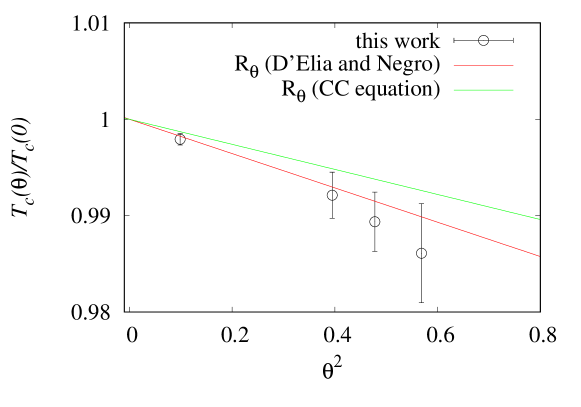
Figure 11: Comparison of our result for $T_{c}(\theta)/T_{c}(0)$ with the result of DElia:2012pvq ; DElia:2013uaf . $R_{\theta}$ obtained through the CC relation is also shown.

Another numerical test is possible by the use of the Clapeyron-Clausius (CC) equation DElia:2013uaf . The application of the equation to the present case is described in Appendix A, from which $R_{\theta}$ is found to be

$$R_{\theta}= {\Delta\chi\over 2\Delta\epsilon}\ ,$$ (17)

where $\Delta\chi=\chi_{L}(T_{c})-\chi_{H}(T_{c})$ and $\chi_{L,H}(T_{c})$ denote the topological susceptibility at the low and high temperature phase at $T=T_{c}$, respectively. For the latent heat, $\Delta\epsilon$, the precise values in the continuum limit are available in Shirogane:2020muc , $\Delta\epsilon/T_{c}^{4}=$1.117(40) for $N_{S}/N_{T}=8$ and 1.349(38) for $N_{S}/N_{T}=6$ . We extrapolate them using a function linear in $N_{T}/N_{S}$ to guess $\Delta\epsilon/T_{c}^{4}\sim 1.813$ for $N_{S}/N_{T}=4$.

For $\Delta\chi$, no data is available. Thus, we try to estimate $\Delta\chi$ as follows. We first divide the configurations at each $\beta_{i}$ into two groups, the low and high temperature phases, by setting the threshold for $\omega$, $\omega_{\rm th}$. Taking $\omega_{\rm th}=0.030$, we calculate the topological susceptibility in each group. Figure 12 shows the $\beta$ dependence of $a^{4}\chi_{L}=\chi(\omega<\omega_{\rm th})$, $a^{4}\chi_{H}=\chi(\omega\geq\omega_{\rm th})$ and $a^{4}\Delta\chi$.

Figure 12: The difference of $a^{4}\chi$ in high and low temperature phases and their difference.

Within the range of $\omega_{\rm th}$ we have studied ($0.028\leq\omega_{\rm th}\leq 0.032$), the variation of $a^{4}\Delta\chi$ is negligibly small. Since the $\beta$ dependence of $a^{4}\Delta\chi$ turns out to be mild, we adopt $a^{4}\Delta\chi=3.6(6)\times 10^{-5}$ at $\beta=2.515$ as the gap at the critical temperature at $\theta=0$.

Substituting $\Delta\epsilon/T_{c}^{4}$ and $a^{4}\Delta\chi$ into (17) leads to

$$R_{\theta}\sim 0.013\ ,$$ (18)

which is reasonably consistent with the value by D’Elia and Negro if we take into account the fact that the mass dimension of $\chi$ is four and tends to be affected by large discretization effects. $R_{\theta}$ thus obtained is shown in Fig. 11. Reasonable consistency with the numerical data for $T_{c}(\theta)/T_{c}(0)$ implies that this way to estimate gaps at the first order transition point can be used, at least, at qualitative level.

It is also possible to use our lattices to estimate $\Delta\epsilon/T_{c}^{4}$ by recalling $\Delta\epsilon/T^{4}=6\,\Delta s_{g}N_{T}^{4}a(d\beta/da)$ Saito:2011fs , where $\Delta s_{g}=s_{gL}-s_{gH}$, the difference of the action density in the low and high temperature phase. Using the above divided configurations at $\beta=2.515$, we obtain $\Delta s_{g}=2.66(12)\times 10^{-4}$, which gives $R_{\theta}\sim 0.0178$.

3.3 free energy density across the transition curve

The $\theta$ dependence of the free energy density is another interesting quantity to study because if it shows a cusp or any other non-analytic behavior it signals a phase transition. However, it is possible to observe such a behavior only after accumulating enough statistics and taking the infinite volume limit. Here, we consider how the free energy density is expected to behave as a function of $\theta$ when it crosses the $T_{c}(\theta)$ curve and try to depict it. To this purpose, we choose the ensemble at $\beta=2.510$ as an example and estimate the free energy density in the lattice unit, $a^{4}f(\theta,T)$, defined by

$$a^{4}f(\theta,T)=\lim_{N_{\rm site}\to\infty}\frac{-1}{N_{\rm site}}\ln\frac{Z(\beta,\theta)}{Z(\beta,0)}=\lim_{N_{\rm site}\to\infty}\frac{-1}{N_{\rm site}}\ln\,\left\langle\,\cos\big{(}\theta\,\hat{Q}\big{)}\,\right\rangle_{\beta}\ .$$ (19)

Since only single lattice size is available in this work, the infinite volume limit is not taken in the following analysis. Unfortunately, the simple implementation of (19) can not detect possible signs of non-analytic behavior as the statistical error and the finiteness of the volume obscure them. Thus, we divide each configuration in the ensemble at $\beta=2.510$ and determine $a^{4}f(\theta,T)$ in each phase through (19).

Figure 13 shows the $\theta$ dependence of the free energy densities. The two curves represent $a^{4}f(\theta,T)$ expected for $\theta\ll 1$ in the two phases, respectively, where $a^{4}\chi_{L,H}$ shown in Fig. 12 are used.

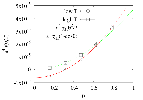
Figure 13: The $\theta$ dependence of the free energy density. The numerical data are obtained at $\beta=2.510$. The expected behaviors in the low and high $T$ phases, $a^{4}\chi_{L}\theta^{2}/2$ and $a^{4}\chi_{H}(1-\cos\theta)$, are shown as a guide to eyes.

According to Tab. 2, the free energy density at $\beta_{c}\sim 2.510$ crosses the $T_{c}(\theta)$ curve around $\theta\sim 2.15\pi/10$. Therefore, in Fig. 13 the data and the curve in the low $T$ phase are shifted in the vertical direction such that the two curves meets there. From the resulting free energy density, it is seen that the ground state transitions from the low to the high $T$ phase as $\theta$ increases from 0.

4 zeros of partition function

When a system experiences a phase transition, the free energy often shows non-analytic behavior, and correspondingly the partition function takes zero in the infinite volume limit. In finite volume, instead zeros appear in unphysical regions of a parameter, known as the Lee-Yang zeros Yang:1952be ; Lee:1952ig or Fischer’s zeros Fischer:1965rna . The aim of this section is to see how the zeros of the partition function associated with phase transitions in the $\theta$-$T$ plane appear. First, following the discussion of Ref. Ejiri:2005ts , let us see the Fischer’s zeros, where $\beta$ is extended to a complex variable as $\beta=\beta_{R}+i\beta_{I}$ and $\beta_{R}$ is fixed to the critical value for a given real $\theta$, $\beta_{R}=\beta_{c}=\beta_{c}(\theta)$. Consider the following ratio of the partition functions and write it in terms of the histogram for $\hat{s}_{g}$ and $\hat{\omega}$ as

$${Z(\beta_{c}+i\beta_{I},\theta)\over Z(\beta_{c},\theta)} ={1\over Z(\beta_{c},\theta)}\int\!\!d\omega\,ds_{g}\,\int{\cal D}U\delta(\hat{\omega}-\omega)\,\delta(\hat{s}_{g}-s_{g})e^{-6(\beta_{c}+i\beta_{I})N_{\rm site}\hat{s}_{g}-i\theta\hat{Q}}$$

$$=\int\!\!d\omega\,ds_{g}\,e^{-6i\beta_{I}N_{\rm site}\,s_{g}}\,p(s_{g},\omega;\beta_{c},\theta)\ .$$ (20)

Assuming the volume to be large enough, when the first order phase transition occurs, the integral of (20) is dominated by two peaks in $p(s_{g},\omega;\beta_{c},\theta_{R})$ around $(s_{g1},\omega_{1})$ and $(s_{g2},\omega_{2})$ with an equal height, i.e. $p(s_{g1},\omega_{1};\beta_{c},\theta_{R})=p(s_{g2},\omega_{2};\beta_{c},\theta_{R})$. Up to an overall constant, (20) is simplified as

$$\ \int\!\!d\omega\,ds_{g}\,e^{-6i\beta_{I}N_{\rm site}\,s_{g}}\,p(s_{g},\omega,Q;\beta_{c},0)$$

$$\approx\left(e^{-6i\beta_{I}N_{\rm site}\,s_{g1}}+e^{-6i\beta_{I}N_{\rm site}\,s_{g2}}\right)\,p(s_{g1},\omega_{1};\beta_{c},\theta_{R})$$

$$\approx 2\,e^{-3i\beta_{I}N_{\rm site}\,(s_{g1}+s_{g2})}\cos\big{(}3\,\beta_{I}N_{\rm site}\,(s_{g1}-s_{g2})\big{)}\,p(s_{g1},\omega_{1};\beta_{c}(\theta_{R}),\theta_{R})\ .$$ (21)

Therefore, $Z(\beta_{c}+i\beta_{I},\theta)$ in (20) vanishes at

$$(\beta_{R},\ \beta_{I})=\left(\beta_{c},\ {\pm(2n+1)\pi\over 6N_{\rm site}(s_{g1}-s_{g2})}\right)\qquad{\rm with}\ n=0,1,2,\cdots\ .$$ (22)

The zeros appear periodically in the imaginary direction, and their interval is inversely proportional to the volume. Therefore, the appearance of two peaks results in these typical signatures for the first order phase transition.

Next, let us explore the Lee-Yang zeros in the complex $\theta$ plane. In the following, $\beta$ is real and $\theta=\theta_{R}+i\theta_{I}$. In this case, the Lee-Yang zeros are found in a specific case. Consider theories in which the histogram of the topological charge at $\theta=0$ follows the Gaussian distribution,

$$p(Q;\beta,0)\sim e^{-\frac{Q^{2}}{2\chi V_{4}}}\ ,$$ (23)

where $V_{4}=a^{4}N_{\rm site}$ denotes the volume of the system under consideration. The following ratio of the partition functions can be written in terms of the histogram for $\hat{Q}$ as

$${Z(\beta,\theta_{R}+i\theta_{I})\over Z(\beta,0)} ={1\over Z(\beta,0)}\sum_{Q}\int\!\!{\cal D}U\,\delta_{\hat{Q},Q}\,e^{-6\beta N_{\rm site}\hat{s}_{g}-i(\theta_{R}+i\theta_{I})\hat{Q}}$$

$$=\sum_{Q}e^{-i(\theta_{R}+i\theta_{I})Q}\,p(Q;\beta,0)\ .$$ (24)

Separating (24) into the real and imaginary part, we try to find the values of $\theta_{R}$ and $\theta_{I}$ where the both parts vanish simultaneously. Using $p(Q;\beta,0)=p(-Q;\beta,0)$, the real part is rewritten as

$${\rm Re}\left[{Z(\beta,\theta_{R}+i\theta_{I})\over Z(\beta,0)}\right]= \ p(0;\beta,0)+\sum_{Q=1}^{\infty}\cos(\theta_{R}Q)\left(e^{+\theta_{I}Q}+e^{-\theta_{I}Q}\right)\,p(Q;\beta,0)\ .$$ (25)

This vanishes if $\theta_{R}$ and $\theta_{I}$ satisfy

$$\cos(\theta_{R}Q)\,e^{-|\theta_{I}|Q}\,p(Q;\beta,0)+\cos(\theta_{R}(Q+k))\,e^{+|\theta_{I}|(Q+k)}\,p(Q+k;\beta,0)=0\ ,$$ (26)

for any integer $Q$ and any positive odd integer $k=2n+1$ with $n=0,1,2,\cdots$. This condition is rewritten as

$$\theta_{I}=\pm\frac{1}{2Q+k}\ln\bigg{(}-\frac{\cos(\theta_{R}Q)}{\cos(\theta_{R}(Q+k))}\frac{p(Q;\beta,0)}{p(Q+k;\beta,0)}\bigg{)}\ .$$ (27)

In order for the argument of the logarithm to be positive,

$$\theta_{R} =(2m+1)\pi\ ,$$ (28)

where $m$ is any integer. Recalling (23), $\theta_{I}$ is eventually found to be

$$\theta_{I}=\pm\frac{2n+1}{2\chi V_{4}}\qquad(n=0,1,2,\cdots)\ .$$ (29)

Next, the imaginary part of (24) is

$${\rm Im}\left[{Z(\beta,\theta_{R}+i\theta_{I})\over Z(\beta,0)}\right]= -\sum_{Q=1}^{\infty}\sin(\theta_{R}Q)\left(e^{+\theta_{I}Q}-e^{-\theta_{I}Q}\right)\,p(Q;\beta,0)\ .$$ (30)

Clearly, it vanishes under (28). Therefore, the partition function of any theories in any dimensions vanishes at

$$(\theta_{R},\ \theta_{I})=\left((2m+1)\pi,\ \frac{2n+1}{2\chi V_{4}}\right)\qquad m,\ n\ :\mbox{ integer}\ ,$$ (31)

as long as the theory has integer topological charge with the Gaussian distribution, (23). The facts that the zeros appear periodically in the imaginary direction and their interval is inversely proportional to the volume tell us that these are the Lee-Yang zeros for the first order phase transition.

Now, the question is whether the distribution (23) is realized in 4d SU($N$) Yang-Mills theory. The large $N$ theory indeed shows (23) in the large volume limit but may not at finite volumes. From the lattice calculation Bonati:2016tvi studying finite volume effects, it is expected that the distribution of $Q$ in the large $N$ limit is, to good approximation, Gaussian even at finite volume and thus the partition function vanishes at (31) to similarly good approximation.

In the large volume limit, the vacuum energy density of the large $N$ Yang-Mills theory is expected to behave with some integer $l$ Witten:1980sp ; Witten:1998uka ; Bonati:2016tvi as

$$\varepsilon(\theta)= \min_{l}\frac{\chi}{2}\left(\theta+2\pi l\right)^{2}\ ,$$ (32)

which has a cusp at $\theta=(2m+1)\pi$ for any integer $m$. These singularities in the large volume limit correspond to the (approximate) zeros at (31) at finite volume.

5 Summary and outlook

We have explored the $\theta$-$T$ phase diagram of four dimensional SU(3) Yang-Mills theory, focusing on the phase boundary, $T_{c}(\theta)$. Instead of measuring the Polyakov loop susceptibility, we employed the histogram method and the constraint effective potential for the Polyakov loop to identify the critical temperature as they provide us with other useful information like the $\theta$ dependence of robustness of the phase transition. Since $\theta$ was introduced through the reweighting method, we could not explore $T_{c}(\theta)$ to $\theta\sim\pi$. The calculations succeeded to $\theta\sim 0.75$ and yielded the results for $T_{c}(\theta)$ consistent with those in DElia:2012pvq ; DElia:2013uaf .

Alternatively, based on the Clapeyron-Clausius equation, one can express $R_{\theta}$ in (16) in terms of the ratio of two gaps at $T=T_{c}(0)$, one being the gap of the topological susceptibility and the other being the latent heat. We divided configurations into the high and low temperature phases and calculated these gaps. For the latent heat, the precise values are available in Shirogane:2020muc ; Borsanyi:2022xml . Combining these gaps, we confirmed the validity of our numerical results. Using those divided configurations, we also depicted the $\theta$ dependence of the free energy density across the first order phase transition.

To study possible phase transitions in the $\theta$-$T$ plane from a different point of view, we examined zeros of partition functions. After recalling how the zeros corresponding to the deconfinement transition appear, those associated with the spontaneous CP violation was studied on the complex $\theta$ plane, and the locations of the Lee-Yang zeros are identified in the large $N$ limit.

There are many points to be improved in the present work. The infinite volume limit and the continuum limit remain to be done to bring the results obtained here to a quantitative level. In order to approach the $\theta=\pi$, it is clearly interesting to combine the histogram method with the subvolume method Kitano:2021jho , which is used to calculate the vacuum energy beyond $\theta=\pi$ in the SU(2) case. Once the whole shape of the $T(\theta)$ curve on the $\theta$-$T$ plane has been determined, we would be able to gain further understandings on the $\theta$ vacuum and field theories.

Appendix A Applying Clapeyron-Clausius equation to the present case

Let $T_{c}(\theta)$ express the curve on the $\theta$-$T$ plane, which separates two phases by first order phase transition. The $\theta$ dependence of $T_{c}(\theta)$ can be expressed in terms of a few measurable quantities by applying Clapeyron-Clausius equation to this system. Following the argument in Shimizu:2007 , we derive the relevant relation below.

We define the free energy density in the high and low temperature phases by $f_{H}(\theta,T)$ and $f_{L}(\theta,T)$, respectively. Note that $f_{H}(\theta,T_{c}(\theta))=f_{L}(\theta,T_{c}(\theta))$. We choose two points close to each other on the critical line $T_{c}(\theta)$, named as $(0,\ T_{c})$ and $(\delta\theta,\ T_{c}+\delta T_{c})$, and calculate the difference of the free energy densities at these points. One can estimate the difference following two paths, one going through the high temperature phase and the other through the low temperature phase as

path 1: $$\ f_{H}(\delta\theta,T_{c}+\delta T_{c})-f_{H}(0,T_{c})={\partial f_{H}(0,T_{c})\over\partial T_{c}}\delta T_{c}+{1\over 2}{\partial^{2}f_{H}(\theta,T_{c})\over\partial\theta^{2}}\bigg{|}_{\theta=0}\delta\theta_{c}^{2}+O(\delta^{2})\ ,$$ (33)

path 2: $$\ f_{L}(\delta\theta,T_{c}+\delta T_{c})-f_{L}(0,T_{c})={\partial f_{L}(0,T_{c})\over\partial T_{c}}\delta T_{c}+{1\over 2}{\partial^{2}f_{L}(\theta,T_{c})\over\partial\theta^{2}}\bigg{|}_{\theta=0}\delta\theta^{2}+O(\delta^{2})\ ,$$ (34)

where $O(\delta^{2})$ representatively expresses $O(\delta T_{c}^{2})$, $O(\delta\theta^{4})$ or $O(\delta T_{c}\delta\theta^{2})$. Note that the symmetry of $f_{H,L}(-\theta,T)=f_{H,L}(\theta,T)$ is used above.

Recalling $f=\epsilon-Ts$ with $\epsilon$ internal energy density and $s$ entropy density and $\partial^{2}f/\partial\theta^{2}|_{\theta=0}=\chi$ and using the fact that the difference (33) and (34) are equal, the following holds up to $O(\delta^{2})$,

$$-s_{H}(0,T_{c})\delta T_{c}+{1\over 2}\chi_{H}\delta\theta^{2}\approx-s_{L}(0,T_{c})\delta T_{c}+{1\over 2}\chi_{L}\delta\theta^{2}\ .$$ (35)

Using the latent heat, $\Delta\epsilon=(s_{H}-s_{L})T_{c}=\epsilon_{H}-\epsilon_{L}$, and noticing that $T_{c}(\delta\theta)/T_{c}(0)=1+\delta T_{c}/T_{c}$, one ends up with

$${T_{c}(\theta)\over T_{c}(0)}\approx 1-{\chi_{L}(T_{c})-\chi_{H}(T_{c})\over 2\Delta\epsilon}\theta^{2}\ .$$ (36)

This relation is derived also in DElia:2013uaf in a similar way.

References

- (1) M. D’Elia and F. Negro, “ dependence of the deconfinement temperature in Yang-Mills theories,” Phys. Rev. Lett. 109, 072001 (2012) doi: 10.1103/PhysRevLett.109.072001 [arXiv:1205.0538 [hep-lat]].
- (2) M. D’Elia and F. Negro, “Phase diagram of Yang-Mills theories in the presence of a term,” Phys. Rev. D 88, no.3, 034503 (2013) doi: 10.1103/PhysRevD.88.034503 [arXiv:1306.2919 [hep-lat]].
- (3) C. G. Callan, Jr., R. F. Dashen and D. J. Gross, “The Structure of the Gauge Theory Vacuum,” Phys. Lett. B 63, 334-340 (1976) doi: 10.1016/0370-2693(76)90277-X
- (4) A. M. Polyakov, “Compact Gauge Fields and the Infrared Catastrophe,” Phys. Lett. B 59, 82-84 (1975) doi: 10.1016/0370-2693(75)90162-8
- (5) A. A. Belavin, A. M. Polyakov, A. S. Schwartz and Y. S. Tyupkin, “Pseudoparticle Solutions of the Yang-Mills Equations,” Phys. Lett. B 59, 85-87 (1975) doi: 10.1016/0370-2693(75)90163-X
- (6) B. J. Harrington and H. K. Shepard, “Periodic Euclidean Solutions and the Finite Temperature Yang-Mills Gas,” Phys. Rev. D 17, 2122 (1978) doi: 10.1103/PhysRevD.17.2122
- (7) D. J. Gross, R. D. Pisarski and L. G. Yaffe, “QCD and Instantons at Finite Temperature,” Rev. Mod. Phys. 53, 43 (1981) doi: 10.1103/RevModPhys.53.43
- (8) J. Frison, R. Kitano, H. Matsufuru, S. Mori and N. Yamada, “Topological susceptibility at high temperature on the lattice,” JHEP 09, 021 (2016) doi: 10.1007/JHEP09(2016)021 [arXiv:1606.07175 [hep-lat]].
- (9) D. Gaiotto, A. Kapustin, Z. Komargodski and N. Seiberg, “Theta, Time Reversal, and Temperature,” JHEP 05, 091 (2017) doi: 10.1007/JHEP05(2017)091 [arXiv:1703.00501 [hep-th]].
- (10) R. Kitano, T. Suyama and N. Yamada, “ in gauge theories,” JHEP 09, 137 (2017) doi: 10.1007/JHEP09(2017)137 [arXiv:1709.04225 [hep-th]].
- (11) G. ’t Hooft, “A Planar Diagram Theory for Strong Interactions,” Nucl. Phys. B 72, 461 (1974) doi: 10.1016/0550-3213(74)90154-0
- (12) E. Witten, “Large N Chiral Dynamics,” Annals Phys. 128, 363 (1980) doi: 10.1016/0003-4916(80)90325-5
- (13) G. ’t Hooft, “Topology of the Gauge Condition and New Confinement Phases in Nonabelian Gauge Theories,” Nucl. Phys. B 190, 455-478 (1981) doi: 10.1016/0550-3213(81)90442-9
- (14) E. Witten, “Theta dependence in the large N limit of four-dimensional gauge theories,” Phys. Rev. Lett. 81, 2862-2865 (1998) doi: 10.1103/PhysRevLett.81.2862 [arXiv:hep-th/9807109 [hep-th]].
- (15) R. Kitano, N. Yamada and M. Yamazaki, “Is Large?,” JHEP 02, 073 (2021) doi: 10.1007/JHEP02(2021)073 [arXiv:2010.08810 [hep-lat]].
- (16) R. Kitano, R. Matsudo, N. Yamada and M. Yamazaki, “Peeking into the vacuum,” Phys. Lett. B 822, 136657 (2021) doi: 10.1016/j.physletb.2021.136657 [arXiv:2102.08784 [hep-lat]].
- (17) L. O’Raifeartaigh, A. Wipf and H. Yoneyama, “The Constraint Effective Potential,” Nucl. Phys. B 271, 653-680 (1986) doi: 10.1016/S0550-3213(86)80031-1
- (18) C. N. Yang and T. D. Lee, “Statistical theory of equations of state and phase transitions. 1. Theory of condensation,” Phys. Rev. 87, 404-409 (1952) doi: 10.1103/PhysRev.87.404
- (19) T. D. Lee and C. N. Yang, “Statistical theory of equations of state and phase transitions. 2. Lattice gas and Ising model,” Phys. Rev. 87, 410-419 (1952) doi: 10.1103/PhysRev.87.410
- (20) M. E. Fischer, “The nature of critical points,” Lect. Theor. Phys. c 7, 1-159 (1965)
- (21) Y. Iwasaki, “Renormalization Group Analysis of Lattice Theories and Improved Lattice Action: Two-Dimensional Nonlinear O(N) Sigma Model,” Nucl. Phys. B 258, 141-156 (1985) doi: 10.1016/0550-3213(85)90606-6
- (22) P. de Forcrand, M. Garcia Perez and I. O. Stamatescu, “Topology of the SU(2) vacuum: A Lattice study using improved cooling,” Nucl. Phys. B 499, 409 (1997) doi: 10.1016/S0550-3213(97)00275-7 [hep-lat/9701012].
- (23) M. Albanese et al. [APE], “Glueball Masses and String Tension in Lattice QCD,” Phys. Lett. B 192, 163-169 (1987) doi: 10.1016/0370-2693(87)91160-9
- (24) M. Okamoto et al. [CP-PACS], “Equation of state for pure SU(3) gauge theory with renormalization group improved action,” Phys. Rev. D 60, 094510 (1999) doi: 10.1103/PhysRevD.60.094510 [arXiv:hep-lat/9905005 [hep-lat]].
- (25) S. Ejiri and N. Yamada, “End Point of a First-Order Phase Transition in Many-Flavor Lattice QCD at Finite Temperature and Density,” Phys. Rev. Lett. 110, no.17, 172001 (2013) doi: 10.1103/PhysRevLett.110.172001 [arXiv:1212.5899 [hep-lat]].
- (26) S. Ejiri et al. [WHOT-QCD], “End point of the first-order phase transition of QCD in the heavy quark region by reweighting from quenched QCD,” Phys. Rev. D 101, no.5, 054505 (2020) doi: 10.1103/PhysRevD.101.054505 [arXiv:1912.10500 [hep-lat]].
- (27) H. Saito, S. Ejiri, S. Aoki, K. Kanaya, Y. Nakagawa, H. Ohno, K. Okuno and T. Umeda, “Histograms in heavy-quark QCD at finite temperature and density,” Phys. Rev. D 89, no.3, 034507 (2014) doi: 10.1103/PhysRevD.89.034507 [arXiv:1309.2445 [hep-lat]].
- (28) A. M. Ferrenberg and R. H. Swendsen, “Optimized Monte Carlo analysis,” Phys. Rev. Lett. 63, 1195-1198 (1989) doi: 10.1103/PhysRevLett.63.1195
- (29) R. Iwami, S. Ejiri, K. Kanaya, Y. Nakagawa, D. Yamamoto and T. Umeda, “Multipoint reweighting method and its applications to lattice QCD,” Phys. Rev. D 92, no.9, 094507 (2015) doi: 10.1103/PhysRevD.92.094507 [arXiv:1508.01747 [hep-lat]].
- (30) M. Shirogane et al. [WHOT-QCD], “Latent heat and pressure gap at the first-order deconfining phase transition of SU(3) Yang-Mills theory using the small flow-time expansion method,” PTEP 2021, no.1, 013B08 (2021) doi: 10.1093/ptep/ptaa184 [arXiv:2011.10292 [hep-lat]].
- (31) S. Borsanyi, Z. Fodor, D. A. Godzieba, R. Kara, P. Parotto and D. Sexty, “Precision study of the continuum SU(3) Yang-Mills theory: how to use parallel tempering to improve on supercritical slowing down for first order phase transitions,” [arXiv:2202.05234 [hep-lat]].
- (32) H. Saito et al. [WHOT-QCD], “Phase structure of finite temperature QCD in the heavy quark region,” Phys. Rev. D 84, 054502 (2011) [erratum: Phys. Rev. D 85, 079902 (2012)] doi: 10.1103/PhysRevD.85.079902 [arXiv:1106.0974 [hep-lat]].
- (33) C. Bonati, M. D’Elia, P. Rossi and E. Vicari, “ dependence of 4D gauge theories in the large- limit,” Phys. Rev. D 94, no. 8, 085017 (2016) doi: 10.1103/PhysRevD.94.085017 [arXiv:1607.06360 [hep-lat]].
- (34) S. Ejiri, “Lee-Yang zero analysis for the study of QCD phase structure,” Phys. Rev. D 73, 054502 (2006) doi: 10.1103/PhysRevD.73.054502 [arXiv:hep-lat/0506023 [hep-lat]].
- (35) S. Ueda, S. Aoki, T. Aoyama, K. Kanaya, H. Matsufuru, S. Motoki, Y. Namekawa, H. Nemura, Y. Taniguchi and N. Ukita, “Development of an object oriented lattice QCD code ’Bridge++’,” J. Phys. Conf. Ser. 523, 012046 (2014) doi: 10.1088/1742-6596/523/1/012046
- (36) A. Shimizu, “Netsugaku no Kiso (Principles of Thermodynamics)”, University of Tokyo Press, 2007 [in Japanese].