STEP: State Estimator for Legged Robots Using a Preintegrated Foot Velocity Factor

Abstract

We propose a novel state estimator for legged robots, STEP, achieved through a novel preintegrated foot velocity factor. In the preintegrated foot velocity factor, the usual non-slip assumption is not adopted. Instead, the end effector velocity becomes observable by exploiting the body speed obtained from a stereo camera. In other words, the preintegrated end effector’s pose can be estimated. Another advantage of our approach is that it eliminates the necessity for a contact detection step, unlike the typical approaches. The proposed method has also been validated in harsh-environment simulations and real-world experiments containing uneven or slippery terrains.

I Introduction

Legged robots are often needed because wheeled robots cannot navigate rough terrains and UAVs cannot carry heavy items due to its payload limitations. As the need for legged robots increases, many studies for accurate state estimation of legged robots have been conducted.

One outstanding research for state estimation of legged robots on unstable and slippery terrain is a stochastic filtering-based method[1]. The key contribution of their approach is the introduction of a leg kinematics constraint during non-slip contact. The effects coming from a possible slip are considered as a Gaussian noise. This framework is still considered a fundamental element of a legged robot’s state estimation. To demonstrate the effectiveness of their approach, they use the contact sensor because the accurate contact detection is necessary for utilizing the leg kinematics constraint.

Figure 1: The legged robot [2] and installed sensor setup for the real-world experiment on gravels. Each robot leg contains three joint encoders. The robot’s body, camera, and foot frames are labelled with $b$, $c$, and $f$, respectively. ${{}^{b}}\boldsymbol{\Gamma}_{{p}}$ and ${{}^{b}}\boldsymbol{\Gamma}_{{R}}$ refer to the translational and rotational transformations from the body frame to the foot frame.

There were attempts to adopt new methodologies or frameworks, such as Invariant Extended Kalman Filter (IEKF) [3, 4], analysis of legged robot’s dynamics [5], optimization on a smooth manifold [6], and preintegration factors [7, 8, 5].

The main advantage of utilizing IEKF is faster convergence and better performance under a wrong initial state [3, 4]. Unfortunately, if the bias is augmented in the state of IEKF, it becomes “imperfect IEKF” named in [3, 9] although this imperfect IEKF outperforms the standard EKF.

A state estimation study has been conducted that considers not only kinematics but also dynamics more efficiently [5], where the authors preintegrate the contact force. However, it is assumed that accurate contact detection is achieved, even if it is considered challenging.

In [6], the robot’s state defined on a smooth manifold was optimized by using the Gauss-Newton method. If a slip occurs (slip can be identified through the speed of the end effector), the leg kinematic factor is ignored.

In addition, similar to the IMU preintegration presented in [10], there were attempts to construct a more robust system by introducing the concept of the preintegrated factor [7, 8, 5]. The authors of [7] proposed preintegrated forward kinematic factor and contact factor, which are adopted in this study. [8] extended [7] by adequately considering the detachment of the foot where the contact was made.

In [11], they developed the loosely coupled state estimator utilizing not only proprioceptive sensors but also a camera and a LiDAR. The robustness and versatility of their approach were demonstrated by using several legged robots for more than two hours of total runtime.

Despite these remarkable studies, the limitations of proprioceptive sensor-based or loosely coupled methods are evident under extreme environments. For instance, the system relying on proprioceptive sensors may diverge on a slippery surface. Similarly, the system that uses loosely coupled camera information easily degraded when significant lighting changes or repetitive patterns appear. Therefore, to develop a more robust and reliable system, there have been many recent attempts for legged robots to couple exteroceptive sensors tightly.

One remarkable study used factor graphs to couple visual odometry and leg odometry tightly [12]. They proposed a novel framework called VILENS. VILENS did not diverge, even if vision degeneracy happened. VILENS was validated on several datasets, including an environment in which illumination was changed. In their following study [13], the body velocity can be calculated based on the non-slip assumption. And, they empirically found that the slip effect can be modeled as a slowly time-varying bias of the body velocity. The body velocities corrected by the bias are preintegrated. The preintegrated measurements constrain the two neighboring poses. Then, this velocity bias was added to the state, resulting in a more robust system. This showed significant improvement compared to their previous approach [12]. These studies are incorporated and detailed in [14]. The main contribution of [14] is that a camera, an IMU, joint encoders, and a LiDAR are tightly fused to achieve more robust operation when the individual sensors would otherwise degraded.

Our previous work, WALK-VIO [15], tightly fuses an inertial sensor, a camera sensor, and joint encoders. The issue that the generated body motion varies with the different controllers was a motivation for developing WALK-VIO. In WALK-VIO, the walking-motion-adaptive leg kinematic constraints that change with the body motion are employed, improving the state estimator’s performance.

Nevertheless, there are still many issues with legged robot state estimation in slippery or uneven terrain. For instance, many researchers assumed that the end effector location is not changed in contact with the ground. This approach is not appropriate if the surface is slippery. Furthermore, the non-slip assumption requires the contact state detection, which needs additional sensors and considerations.

The contact detection methods can be classified as to whether the contact sensor is used or not. In contact sensor-based methods, several limitations exist [16]. First, due to the aggressive motions of legged robots and the impacts at the feet, the sensors would be damaged over repeated use. Second, a heavy protector for the sensor is required. Thus, to utilize the leg kinematics constraint, detecting the contact without using the contact sensor is preferred.

The ground reaction force (GRF) analysis is typically used for contact estimation without contact sensors. In [17], through a detailed analysis of GRF parameters, invalid leg odometry was discarded. Moreover, [16] proposed a probabilistic way to detect contact, which was extended to the Hidden Markov Model (HMM) based probabilistic slip estimator[18]. This approach has been demonstrated by operating ANYmal [19] on ice.

Even though several studies not using contact sensors have been published, an additional computation is required for any contact detection. Furthermore, the possibility of mis-detecting the contact cannot be ignored in a harsh environment, such as muddy or slippery surfaces. Even though previous studies assumed the slip effect could be modeled as Gaussian noise (or bias), this approach might be invalid under severe slip. As long as we adopt the above assumptions, the accurate contact detector is essential.

However, in this research, those assumptions are not adopted when establishing leg kinematics. Thus, the proposed algorithm can be utilized even in harsh environments, thereby broadening its application. This letter proposes a novel state estimator, STEP (STate Estimator using Preintegrated foot velocity factor), that does not rely on an accurate contact detector and does not assume that the foot’s position is fixed in contact. This letter makes the following contributions:

• We present a novel preintegrated foot velocity factor that can be exploited regardless of contact state. This factor can constrain the foot pose between the consecutive image frames, which results in the improvement in the optimization of the overall cost function.

• The end effector velocity is estimated from leg kinematics. Note that we do not use the non-slip assumption. Thus, it is independent of ground characteristics, such as the friction coefficient.

• The performance of STEP was evaluated in harsh simulation environments and with real experimental datasets.

II Preliminaries

In this section, preliminaries of Lie groups and associated Lie Algebra are briefly presented for the following sections. More information on Lie group and Lie algebra can be found in [10, 20, 21, 22]. Especially, [10] is recommended for better understanding of this letter.

II-A Useful Properties of Matrix Lie Group

In the section, we consider the matrix Lie group $\mathcal{G}$ closed under matrix multiplication [22]. Specifically, we are interested in the rotation matrix, an element of Lie group, especially special orthogonal group. The rotation matrix in 3D space is formally defined as follows:

$$\mathrm{SO}(3)=\left\{\mathbf{R}\in\mathrm{GL}_{3}(\mathbb{R})\mid\mathbf{R}^{\top}\mathbf{R}=\mathbf{I}_{3\times 3},\operatorname{det}\mathbf{R}=1\right\},\vspace{-1mm}$$ (1)

where $\mathbf{R}$ is the rotation matrix, an element of $\mathrm{GL}_{3}(\mathbb{R})$, general linear group of degree 3 and $\mathbf{I}_{3\times 3}$ is the $3\times 3$ identity matrix.

The associated Lie algebra is denoted by $\mathfrak{g}$. The linear hat operator, $(\cdot)^{\wedge}:\mathbb{R}^{m}\rightarrow\mathfrak{g}$, maps a vector to the Lie algebra. The tangent space to the smooth manifold, $\mathrm{SO}(3)$, (at the identity of $\mathcal{G}$) is denoted as $\mathfrak{so}(3)$, which is the associated Lie algebra and coincides with the space of 3 $\times$ 3 skew symmetric matrices. As described in [10], by adopting the hat operator, Lie algebra can be vectorized for convenience as follows:

$$\boldsymbol{\phi}^{\wedge}=\left[\begin{array}[]{c}\phi_{1}\\ \phi_{2}\\ \phi_{3}\end{array}\right]^{\wedge}=\left[\begin{array}[]{ccc}0&-\phi_{3}&\phi_{2}\\ \phi_{3}&0&-\phi_{1}\\ -\phi_{2}&\phi_{1}&0\end{array}\right]\in\mathfrak{so}(3).$$ (2)

A useful property of $(\cdot)^{\wedge}$, anticommutative property is introduced:

$$\mathbf{a}^{\wedge}\mathbf{b}=-\mathbf{b}^{\wedge}\mathbf{a}\quad\forall\mathbf{a},\mathbf{b}\in\mathbb{R}^{3}.\vspace{-2mm}$$ (3)

For the corresponding inverse map, vee operator is introduced as $(\cdot)^{\vee}:\mathfrak{g}\rightarrow\mathbb{R}^{m}$. The hat operator and the vee operator have the following relationship$:\mathbf{R}={\mathbf{a}}^{\wedge}$ then $\mathbf{R}^{\vee}=\mathbf{a}$. More information can be found in [10].

The exponential map, $\operatorname{exp}:\mathfrak{so}(3)\rightarrow\mathrm{SO}(3)$, is defined as follows:

$$\exp\left(\boldsymbol{\phi}^{\wedge}\right)=\mathbf{I}_{3\times 3}+\frac{\sin(\|\boldsymbol{\phi}\|)}{\|\boldsymbol{\phi}\|}\boldsymbol{\phi}^{\wedge}+\frac{1-\cos(\|\boldsymbol{\phi}\|)}{\|\boldsymbol{\phi}\|^{2}}\left(\boldsymbol{\phi}^{\wedge}\right)^{2}.$$ (4)

It is often approximated that $\exp\left(\boldsymbol{\phi}^{\wedge}\right)\approx\mathbf{I}_{3\times 3}+\boldsymbol{\phi}^{\wedge}$, where $\boldsymbol{\phi}\approx 0$.

Likewise, for any $\|\boldsymbol{\phi}\|<\pi$, the logarithm map, $\operatorname{log}:\mathrm{SO}(3)\rightarrow\mathfrak{so}(3)$, which associates a Lie group element $\mathbf{R}\neq\mathbf{I}_{3\times 3}$ in $\mathrm{SO}(3)$ to a Lie algebra element is defined as follows:

$$\small\log(\mathbf{R})=\frac{\varphi\cdot\left(\mathbf{R}-\mathbf{R}^{\top}\right)}{2\sin(\varphi)}\text{ with }\varphi=\cos^{-1}\left(\frac{\operatorname{tr}(\mathbf{R})-1}{2}\right).$$ (5)

Note that it represents the rotation by using the rotation axis and the rotation angle: $\operatorname{log}(\mathbf{R})^{\vee}=\mathbf{a}\phi$, where $\mathbf{a}$ and $\phi$ are the rotation axis and the rotation angle of $\mathbf{R}$, respectively. If $\mathbf{R}=\mathbf{I}_{3\times 3}$, then the rotation angle, $\phi=0$ and the rotation axis, $\mathbf{a}$, can be chosen arbitrarily.

Similar to the vectorization of Lie algebra above, the exponential and logarithm map is vectorized as below [10]:

$$\operatorname{Exp}:\mathbb{R}^{3}\rightarrow\mathrm{SO}(3)\quad;\boldsymbol{\phi}\mapsto\exp\left(\boldsymbol{\phi}^{\wedge}\right)$$ (6)

$$\operatorname{Log}:\mathrm{SO}(3)\rightarrow\mathbb{R}^{3}\quad;\mathbf{R}\mapsto\log(\mathbf{R})^{\vee}.$$

Later, for small $\delta\boldsymbol{\phi}$, the following first-order approximation will be used:

$$\vspace{-1mm}\operatorname{Exp}(\boldsymbol{\phi}+\delta\boldsymbol{\phi})\approx\operatorname{Exp}(\boldsymbol{\phi})\operatorname{Exp}\left(\mathbf{J}_{r}(\boldsymbol{\phi})\delta\boldsymbol{\phi}\right),$$ (7)

$$\vspace{-1mm}\operatorname{Log}(\operatorname{Exp}(\boldsymbol{\phi})\operatorname{Exp}(\delta\boldsymbol{\phi}))\approx\boldsymbol{\phi}+\mathbf{J}_{r}^{-1}(\boldsymbol{\phi})\delta\boldsymbol{\phi},$$ (8)

$$\operatorname{Exp}(\delta\boldsymbol{\phi})\approx\mathbf{I}+(\delta\boldsymbol{\phi})^{\wedge},\vspace{-1mm}$$ (9)

where $\mathbf{J}_{r}(\boldsymbol{\phi})$ is right Jacobian. The derivation of $\mathbf{J}_{r}(\boldsymbol{\phi})$ can be found in [20, 10] as follows:

$$\small\mathbf{J}_{r}(\boldsymbol{\phi})=\mathbf{I}-\frac{1-\cos(\|\boldsymbol{\phi}\|)}{\|\boldsymbol{\phi}\|^{2}}\boldsymbol{\phi}^{\wedge}+\frac{\|\boldsymbol{\phi}\|-\sin(\|\boldsymbol{\phi}\|)}{\left\|\boldsymbol{\phi}^{3}\right\|}\left(\boldsymbol{\phi}^{\wedge}\right)^{2}.\normalsize$$ (10)

Lastly, another property of the exponential map of $\mathrm{SO}$(3) is introduced:

$$\vspace{-1mm}\mathbf{R}\operatorname{Exp}(\boldsymbol{\phi})\mathbf{R}^{\top}=\operatorname{exp}\left(\mathbf{R}\boldsymbol{\phi}^{\wedge}\mathbf{R}^{\top}\right)=\operatorname{Exp}(\mathbf{R}\boldsymbol{\phi}),$$ (11)

$$\operatorname{Exp}(\boldsymbol{\phi})\mathbf{R}=\mathbf{R}\operatorname{Exp}\left(\mathbf{R}^{\top}\boldsymbol{\phi}\right).$$ (12)

II-B Uncertainty Description on a Smooth Manifold

One advantage of representing the rotation as the Lie group and the associated Lie algebra is that uncertainty can be described without losing the Gaussian property [10]. The uncertainty in $\mathrm{SO}(3)$ is modeled by defining a noise distribution in the tangent space, its Lie algebra $\mathfrak{so}(3)$, and then mapping it to $\mathrm{SO}(3)$ through the exponential map [7, 10], which will be explained in the following section. The perturbed rotation matrix can be written as follows:

$$\tilde{\mathbf{R}}=\mathbf{R}\operatorname{Exp}\left(\delta\boldsymbol{\phi}\right),\quad\delta\boldsymbol{\phi}\sim\mathcal{N}(0,\boldsymbol{\Omega}),\vspace{-1mm}$$ (13)

where $\delta\boldsymbol{\phi}$ is a normally distributed small perturbation with zero mean and covariance $\boldsymbol{\Omega}$, and ${\mathbf{R}}$ is the noise-free rotation. The detailed derivation of the distribution of $\mathbf{R}$ is indicated in [23, 10]. We adopt the result of the negative log-likelihood $\mathcal{L}$ of a rotation $\mathbf{R}$ given a noisy measurement $\tilde{\mathbf{R}}$:

$$\mathcal{L}({\mathbf{R}})\propto\frac{1}{2}\left\|\operatorname{Log}\left({\mathbf{R}}^{-1}\tilde{\mathbf{R}}\right)\right\|_{\boldsymbol{\Sigma}}^{2}=\frac{1}{2}\left\|\operatorname{Log}\left(\tilde{\mathbf{R}}^{-1}{\mathbf{R}}\right)\right\|_{\boldsymbol{\Sigma}}^{2}.$$ (14)

The uncertainty of translation can be characterized by exploiting the additive Gaussian noise assumptions [10].

II-C Optimization on a Smooth Manifold

We could not directly apply vector calculus to the body orientation involved in the state that evolves on the $\mathrm{SO}(3)$ manifold. Thus, we adopt the approach suggested in [10, 6], called the lift-solve-retract scheme. Furthermore, for the required retraction for $\mathrm{SO}$(3) and lifting for $\mathfrak{so}$(3), $\operatorname{Exp}(\cdot)$ and $\operatorname{Log}(\cdot)$ maps are adopted, which are introduced in Section II-A.

III Factor Graph Formulation

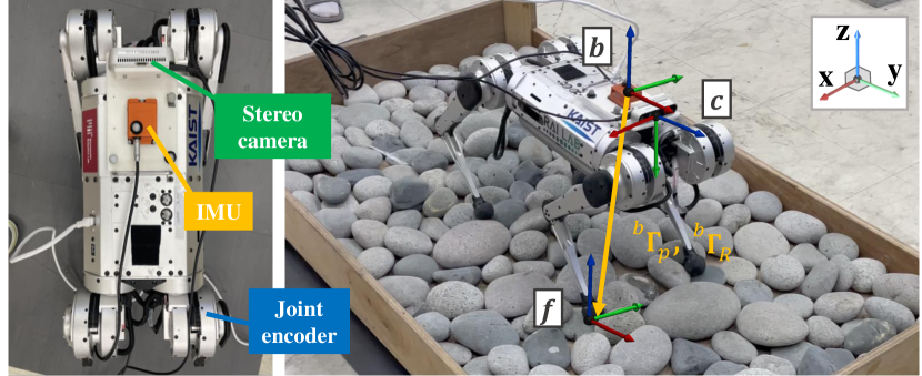
In this section, we explain the factor graph formulation of STEP. The factor graph is based on that of the VINS-Fusion [24] framework, which is a tightly coupled, sliding-window nonlinear optimization-based VIO algorithm. To construct a state estimator for legged robots, we added a novel preintegrated foot velocity factor to the factor graph. In addition, we modified VINS-Fusion to optimize the factor graph on-manifold. As shown in Fig. 1, a sensor configuration consisting of a stereo camera, an IMU sensor, and joint encoders for each leg was used, and the contact sensor was not used. The body frame was located on the IMU.

III-A State Definition

The state vector used in this research is as follows:

$$\begin{split}&\mathcal{X}=[\mathbf{x}_{0},\mathbf{x}_{1},\cdots,\mathbf{x}_{i-1},\lambda_{0},\lambda_{1},\cdots,\lambda_{k}],\\ &\mathbf{x}_{i}=[\mathbf{p}^{w}_{b_{i}},\mathbf{R}^{w}_{b_{i}},\mathbf{v}^{w}_{b_{i}},\mathbf{\Psi}^{w}_{l,i},\mathbf{s}^{w}_{l,i},\mathbf{b}^{a}_{i},\mathbf{b}^{g}_{i}],\end{split}\vspace{-3mm}$$ (15)

where $\mathbf{x}_{i}$ represents the robot state when the $i$-th keyframe is input. It contains the body position, $\mathbf{p}^{w}_{b_{i}}\in\mathbb{R}^{3}$; orientation $\mathbf{R}^{w}_{b_{i}}\in\mathrm{SO}(3)$; velocity, $\mathbf{v}^{w}_{b_{i}}\in\mathbb{R}^{3}$; orientation of the $l$-th end effector, $\mathbf{\Psi}^{w}_{l,i}$; position of the $l$-th end effector, $\mathbf{s}^{w}_{l,i}$; the IMU accelerometer and gyroscope biases, $\mathbf{b}^{a}_{i}\in\mathbb{R}^{3}$ and $\mathbf{b}^{g}_{i}\in\mathbb{R}^{3}$; and $\lambda_{k}$ indicates the $k$-th inverse depth of the viusual feature in the first observed camera frame. Note that the superscript $w$ denotes the parameters are estimated in the world frame. For readability throughout this letter, however, the world frame superscripts will be dropped. For example, $\mathbf{p}^{w}_{b_{i}}$, $\mathbf{v}^{w}_{b_{i}}$, and $\mathbf{R}^{w}_{b_{i}}$ will be abbreviated as ${\mathbf{p}_{i}}$, ${\mathbf{v}_{i}}$, and $\mathbf{R}_{i}$, respectively. If it is not represented in the world frame, then a reference frame is denoted by a left side superscript, such as the body frame ${{}^{b}}(\cdot)$, the camera frame ${{}^{c}}(\cdot)$, and the foot frame ${{}^{f}}(\cdot)$. Lastly, $\tilde{(\cdot)}$ denotes the noisy measurement.

Figure 2: The visualization of the factor graph structure. The factor graph consists of measurement factors: (1) prior factor, (2) IMU factor, (3) visual factor, (4) forward kinematics factor, and (5) preintegrated foot velocity factor. Unlike the forward kinematics factor, the preintegrated foot velocity factor can relate the foot pose between the consecutive frames.

III-B Measurements and Factor Graph

The sensors used in this letter are a stereo camera, IMU, and leg joint encoders. All measurements from each sensor up to the $k$-th keyframe, $\mathcal{Z}_{k}$, can be represented as follows:

$$\tiny\mathcal{Z}_{k}=\displaystyle\bigcup_{\forall{(i,j)}\in\mathcal{T}_{k}}\{\mathcal{I}_{ij},\mathcal{C}_{i},{\mathcal{K}}^{l}_{i},{\mathcal{V}}^{l}_{ij}\},l=\left\{1,\ldots N\right\},\vspace{-1.5mm}$$

where $\mathcal{T}_{k}$ is the set of timestamps of the keyframe in the $k$-th sliding window. We assume the IMU and joint encoders are synchronized with the camera. Furthermore, $\mathcal{I}_{ij}\in\mathbb{R}^{6}$ refers to the preintegrated IMU measurement between timestamps $i$ and $j$; $\mathcal{C}_{i}$ is the keyframe obtained at time $i$; $\mathcal{K}^{l}_{i}\in\mathbb{R}^{n_{\mathrm{joints}}}$ is the forward kinematic measurement of the $l$-th leg at time $i$, where $n_{\mathrm{joints}}$ denotes the number of joints. $\mathcal{V}^{l}_{ij}\in\mathbb{R}$ denotes the foot velocity measurement of the $l$-th leg between $i$ and $j$, which is obtained from leg kinematics.

The IMU and joint encoder measurements are input at higher frequencies. So, the IMU measurements are preintegrated, as proposed in[10]. For similar reasons, the joint measurements are preintegrated and used for tracking the pose of the $l$-th end effector between two frames. A detailed description of the preintegration of foot velocity will be given in Section IV.

III-C Cost Function

If all sensor measurements are conditionally independent to each other, the maximum posterior state $\mathcal{X}_{k}$, given the measurement $\mathcal{Z}_{k}$, can be expressed as:

$$\mathcal{X}^{*}_{k}=\operatorname*{arg\,max}_{\mathcal{X}_{k}}p\big{(}\mathcal{X}_{k}\big{|}\mathcal{Z}_{k}\big{)}\propto p\big{(}\mathcal{X}_{0}\big{)}p\big{(}\mathcal{Z}_{k}\big{|}\mathcal{X}_{k}\big{)},\vspace{-1mm}$$ (16)

where $p\big{(}\mathcal{Z}_{k}\big{|}\mathcal{X}_{k}\big{)}=\prod_{(i,j)\in\mathcal{T}_{k}}p\big{(}\mathcal{I}_{ij}\big{|}\mathcal{X}_{j}\big{)}p\big{(}\mathcal{C}_{i}\big{|}\mathcal{X}_{i}\big{)}p\big{(}\mathcal{K}_{i}\big{|}\mathcal{X}_{i}\big{)p\big{(}\mathcal{V}_{ij}\big{|}\mathcal{X}_{j}\big{)}}.$

(16) can be transformed into an equivalent nonlinear least-square problem. Therefore, the final objective we used for obtaining a maximum posteriori estimate of $\mathcal{X}_{k}$ can be formulated as follows:

$$\begin{gathered}\min_{\mathcal{X}_{k}}\Bigg{\{}\parallel{\color[rgb]{0,0,0}\mathbf{r}_{p}-\mathbf{H}_{p}\mathcal{X}_{k}}\parallel^{2}+\sum_{(i,j)\in\mathcal{T}_{k}}\parallel{\color[rgb]{0,0,0}{\mathbf{r}_{\mathcal{I}}(\mathcal{I}_{ij},\mathcal{X}_{k})}}\parallel_{\mathbf{\Omega}_{\mathcal{I}_{ij}}}^{2}+\\ \sum_{i\in\mathcal{T}_{k}}\sum_{n\in\mathcal{F}}\rho(\parallel{\color[rgb]{0,0,0}{\mathbf{r}_{\mathcal{C}}(\mathcal{C}_{i,\mathbf{f}_{n}},\mathcal{X}_{k})}}\parallel_{\mathbf{\Omega}_{\mathcal{C}_{i,n}}}^{2})+\sum_{i\in\mathcal{T}_{k}}\sum_{l=1}^{N}\parallel{\color[rgb]{0,0,0}{\mathbf{r}_{\mathcal{K}}(\mathcal{K}^{l}_{i},\mathcal{X}_{k})}}\parallel_{\mathbf{\Omega}_{\mathcal{K}_{i,l}}}^{2}\\ +\sum_{(i,j)\in\mathcal{T}_{k}}\sum_{l=1}^{N}\parallel{\color[rgb]{0,0,0}{\mathbf{r}_{\mathcal{V}}(\mathcal{V}^{l}_{ij},\mathcal{X}_{k})}}\parallel_{\mathbf{\Omega}_{\mathcal{V}_{ij,l}}}^{2}\Bigg{\}},\end{gathered}$$ (17)

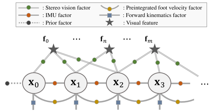
where $\mathcal{F}$ is the set of visual feature indices. Each sensor noise covariance is expressed as $\mathbf{\Omega}_{\mathcal{I}_{ij}},\mathbf{\Omega}_{\mathcal{C}_{i,n}}$, $\mathbf{\Omega}_{\mathcal{K}_{i,l}}$, and $\mathbf{\Omega}_{\mathcal{V}_{ij,l}}$. In addition, $\parallel\cdot\parallel$ refers to the Mahalanobis norm, and $\rho(\cdot)$ refers to the Huber norm [25]. The cost function is defined as the sum of each measurement factor: (1) prior factor $\mathbf{r}_{0}$, (2) IMU factor $\mathbf{r}_{\mathcal{I}}$, (3) visual factor $\mathbf{r}_{\mathcal{C}}$, (4) forward kinematics factor $\mathbf{r}_{\mathcal{K}}$, and (5) preintegrated foot velocity factor $\mathbf{r}_{\mathcal{V}}$. For solving the nonlinear least square problem, Levenberg-Marquardt algorithm[26] is used. The visualization of the corresponding factor graph is shown in Fig.  2.

III-D VIO Factors

In this section, each factor forming the cost function is described. The prior factor and visual factor are adopted from [24]. The IMU factor is from [10]. The leg kinematic-related factors such as the forward kinematics factor and preintegrated foot velocity factor will be explained in Section IV.

1) Prior factor: Due to the computational cost, a sliding window-based method is adopted. Therefore, a prior factor is used to serve as an anchor whenever marginalization occurs. The prior factor $\mathbf{r}_{0}$ is defined as the error between the prior state $\mathbf{x}_{0}$ and the estimated prior state $\mathbf{\hat{x}}_{0}$.

2) IMU factor: Since the IMU usually offers data with a higher frequency than the camera, the measurements between the frames are preintegrated to compute the changes in pose $\Delta\mathbf{\tilde{p}}$, velocity $\Delta\mathbf{\tilde{v}}$, and orientation $\Delta\mathbf{\tilde{R}}$ of the robot. And these changes can constrain the two neighboring nodes of the graph by defining the IMU factor $\mathbf{r}_{\mathcal{I}}$ given IMU measurements $\mathcal{I}_{ij}$ as follows:

$$\footnotesize\mathbf{r}_{\mathcal{I}}(\mathcal{I}_{ij},\mathcal{X}_{k})=\begin{pmatrix}\mathbf{R}^{\top}_{i}(\mathbf{p}_{j}-\mathbf{p}_{i}-\mathbf{v}\Delta t_{j}-\frac{1}{2}\mathbf{g}\Delta t^{2}_{j})-\Delta\tilde{\mathbf{p}}_{j}\\ \mathbf{R}^{\top}_{i}(\mathbf{v}_{j}-\mathbf{v}_{i}-\mathbf{g}\Delta t_{j})-\Delta\tilde{\mathbf{v}}_{j}\\ \operatorname{Log}\big{(}\Delta{\tilde{\mathbf{R}}_{j}}\mathbf{R}^{\top}_{i}\mathbf{R}_{j}\big{)}\\ \mathbf{b}^{a}_{j}-\mathbf{b}^{a}_{i}\\ \mathbf{b}^{g}_{j}-\mathbf{b}^{g}_{i}\end{pmatrix}.\vspace{-1mm}$$ (18)

The IMU factor is adopted from [10], but we do not consider the bias update between consecutive keyframes due to computational complexity.

3) Visual factor: For the visual factor, the traditional reprojection error is utilized. The visual factor $\mathbf{r}_{\mathcal{C}}$ when the 3D feature $\mathbf{f}_{n}$ observed in the $i$-th frame is defined as:

$$\mathbf{r}_{\mathcal{C}}(\mathcal{C}_{i,\mathbf{f}_{n}},\mathcal{X}_{k})=\textbf{\emph{f}}_{i,n}-\pi\big{(}\mathbf{R}_{i},\mathbf{p}_{i},\mathbf{f}_{n}\big{)},\vspace{-1mm}$$ (19)

where $\pi(\cdot)$ is the projection function which projects the 3D feature to the image and $\textbf{\emph{f}}_{i,n}$ is the $n$-th feature observed in the $i$-th frame.

IV Leg Factors

This section presents the novel preintegrated foot velocity factor, which is our key contribution, and the forward kinematics factor. As we introduced in Section I, many researchers have proposed various leg factors constrained by non-slip assumption. Additionally, most of them considered the effect of sensor noises or slippage as a Gaussian noise or bias. However, those techniques might fail to estimate the end effector pose in a severe slippage condition, which leads to deteriorating the estimated body pose tightly coupled to the end effector pose. In addition, they can constrain the pose only when the contact state is maintained for a certain period, and it would be vulnerable to the slip occurrences. Therefore, we propose a preintegrated foot velocity factor that does not depend on the contact state and that can be used at all times. For this, the changes in foot pose between consecutive frames are calculated by preintegrating the end effector velocities.

IV-A Measurement Model

In this section, foot linear and angular velocities are derived in the foot frame, which is necessary for later preintegration of foot linear and angular velocity. To this end, forward kinematics of a legged robot and transformation between frames are exploited.

The joint encoder measurement vector $\tilde{\boldsymbol{\alpha}}(t)$ can be expressed as follows:

$$\tilde{\boldsymbol{\alpha}}(t)=\boldsymbol{\alpha}(t)+\mathbf{n}^{\alpha}(t)\in\mathbb{R}^{M},\vspace{-2mm}$$ (20)

where $\boldsymbol{\alpha}(t)$ is the true joint angle; $\mathbf{n}^{\alpha}(t)\sim\mathcal{N}(0,\boldsymbol{\Omega}^{\alpha})$ is the joint measurement noise modeled as a Gaussian noise with covariance $\boldsymbol{\Omega}^{\alpha}$; and $M$ is the number of joint encoders of each leg.

When $\tilde{\boldsymbol{\alpha}}(t)$ is given, by using the leg kinematics model, the foot position $\mathbf{s}(t)\in\mathbb{R}^{3}$ and orientation $\mathbf{\Psi}(t)\in\mathrm{SO}(3)$ in the world frame at $t$ can be calculated as follows:

$$\mathbf{\Psi}(t)=\mathbf{R}(t)\,{{}^{b}}\boldsymbol{\Gamma}_{{R}}(\boldsymbol{\alpha}(t))=\mathbf{R}(t)\,{{}^{b}}\boldsymbol{\Gamma}_{{R}}(\tilde{\boldsymbol{\alpha}}(t)-\mathbf{n}^{\alpha}(t))$$ (21)

$$\begin{split}\mathbf{s}(t)&=\mathbf{R}(t)\,{{}^{b}}\boldsymbol{\Gamma}_{{p}}(\boldsymbol{\alpha}(t))+\mathbf{p}(t)\\ &=\mathbf{R}(t){{}^{b}}\boldsymbol{\Gamma}_{{p}}(\tilde{\boldsymbol{\alpha}}(t)-\mathbf{n}^{\alpha}(t))+\mathbf{p}(t),\end{split}$$ (22)

where ${{}^{b}}\boldsymbol{\Gamma}_{p}(\cdot)$ and ${{}^{b}}\boldsymbol{\Gamma}_{R}(\cdot)$ are the end effector position and orientation calculated by forward kinematics, respectively [7]. Note that ${{}^{b}}\boldsymbol{\Gamma}_{p}(\cdot)$ and ${{}^{b}}\boldsymbol{\Gamma}_{R}(\cdot)$ are expressed in the body frame. From now on, we omit $t$ for brevity.

To represent the foot angular velocity in the foot frame, we differentiate (21) on both sides:

$$\dot{\boldsymbol{\Psi}}=\mathbf{R}{(^{b}{\mathbf{w}})}^{\wedge}\,{{}^{b}}\boldsymbol{\Gamma}_{R}({\boldsymbol{\alpha}})+\mathbf{R}\,{{}^{b}}\boldsymbol{\Gamma}_{R}({\boldsymbol{\alpha}}){({{}^{b}}\boldsymbol{\omega})}^{\wedge},\vspace{-1mm}$$ (23)

where ${}^{b}{\mathbf{w}}$ is the body angular velocity, and ${{}^{b}}\boldsymbol{\omega}$ the foot angular velocity expressed in the body frame. Note that ${{}^{b}}\boldsymbol{\omega}$ can be computed because of leg kinematics.

Alternatively, the derivative of $\boldsymbol{\Psi}$ can be represented as the multiplication of foot orientation and foot angular velocity:

$$\dot{\boldsymbol{\Psi}}=\boldsymbol{\Psi}{({{}^{f}}{\boldsymbol{\omega}})}^{\wedge},\vspace{-1mm}$$ (24)

where ${{}^{f}}{\boldsymbol{\omega}}$ is the foot angular velocity represented in the foot frame.

Using (23) and (24), we can write ${{}^{f}}{\boldsymbol{\omega}}$ as a function of ${{}^{b}}{\mathbf{w}}$, ${\boldsymbol{\alpha}}$, and ${}^{b}{{\boldsymbol{\omega}}}$. For the sake of simplicity, we omit ${\boldsymbol{\alpha}}$ from now on:

$${{}^{f}}{\boldsymbol{\omega}}={({{}^{b}}\boldsymbol{\Gamma}_{R}^{\top}{({{{}^{b}}{\mathbf{w}}})}^{\wedge}\,{{}^{b}}\boldsymbol{\Gamma}_{R}+{(^{b}{\boldsymbol{\omega}})}^{\wedge})}^{\vee}.$$ (25)

(25) can be written with sensor measurements as follows:

$${{}^{f}}{\tilde{\boldsymbol{\omega}}}={({{}^{b}}\boldsymbol{\Gamma}_{R}^{\top}{({{{}^{b}}{\tilde{\mathbf{w}}-\mathbf{b}^{g}}})}^{\wedge}\,{{}^{b}}\boldsymbol{\Gamma}_{R}+{(^{b}{\tilde{\boldsymbol{\omega}}})}^{\wedge})}^{\vee}+\mathbf{n}^{\tilde{\boldsymbol{\omega}}},$$ (26)

where $\mathbf{n}^{\tilde{\boldsymbol{\omega}}}$ is the single noise term with covariance $\boldsymbol{\Omega}^{{\tilde{\boldsymbol{\omega}}}}$ that combines the effects of gyro measurement noise, joint encoder noise, and imprecise kinematic modeling. This strategy is inspired by [1] and [7].

Likewise, $\dot{\mathbf{s}}$ can be interpreted as a foot linear velocity expressed in the world frame, written as follows:

$$\dot{\mathbf{s}}={\boldsymbol{\nu}}=\mathbf{R}{({{}^{b}}{\mathbf{w}})}^{\wedge}\,{{}^{b}}\boldsymbol{\Gamma}_{p}+\mathbf{R}\mathbf{J}_{p}{{{\dot{\boldsymbol{\alpha}}}}}+\mathbf{v},\vspace{-1mm}$$ (27)

where ${\boldsymbol{\nu}}$ is the foot velocity expressed in the world frame; $\mathbf{J}_{p}=\frac{\delta{{}^{b}}\boldsymbol{\Gamma}_{p}\left({\boldsymbol{\alpha}}\right)}{\delta{\boldsymbol{\alpha}}}$; and $\mathbf{v}$ is the body velocity represented in the world frame.

Note that (27) should be transformed to the foot frame and expressed with sensor measurements to find the preintegrated foot measurement. We manipulate (27) by multiplying $\boldsymbol{\Psi}^{\top}$ to both sides and augmenting the measurements, leading to:

$$\begin{split}{{}^{f}}\tilde{\boldsymbol{\nu}}&={{}^{b}}\boldsymbol{\Gamma}_{R}^{\top}{(^{b}\tilde{\mathbf{w}}-\mathbf{b}^{g})}^{\wedge}\,{{}^{b}}\boldsymbol{\Gamma}_{p}+{{}^{b}}\boldsymbol{\Gamma}_{R}^{\top}\mathbf{J}_{p}{{\tilde{\dot{\boldsymbol{\alpha}}}}}+{{}^{b}}\boldsymbol{\Gamma}_{R}^{\top}\mathbf{R}^{\top}\mathbf{v}+\mathbf{n}^{\tilde{\boldsymbol{\nu}}}\\ &\simeq{{}^{b}}\boldsymbol{\Gamma}_{R}^{\top}{(^{b}\tilde{\mathbf{w}}-\mathbf{b}^{g})}^{\wedge}\,{{}^{b}}\boldsymbol{\Gamma}_{p}+{{}^{b}}\boldsymbol{\Gamma}_{R}^{\top}\mathbf{J}_{p}{{\tilde{\dot{\boldsymbol{\alpha}}}}}+{{}^{f}}\tilde{\mathbf{v}}+\mathbf{n}^{\tilde{\boldsymbol{\nu}}},\end{split}$$ (28)

where ${{}^{f}}\tilde{\mathbf{v}}$ is the body velocity measurement transformed to the foot frame and $\mathbf{n}^{\tilde{\boldsymbol{\nu}}}$ is the noise term of ${{}^{f}}\tilde{\boldsymbol{\nu}}$ with covariance $\boldsymbol{\Omega}^{\tilde{\boldsymbol{\nu}}}$, which can be written as in (26). Note that we assume that $\mathbf{n}^{\tilde{\boldsymbol{\omega}}}$ and $\mathbf{n}^{\tilde{\boldsymbol{\nu}}}$ are Gaussian white noises.

For foot velocity preintegration, we stress that $\mathbf{R}^{\top}\mathbf{v}$ in (28) can be approximated by the body velocity measurement obtained from a stereo vision with optical flow analysis as follows [27]:

$${}^{b}\tilde{\mathbf{v}}=\mathbf{R}_{c}^{b}~{}{{}^{c}}\tilde{\mathbf{v}},$$ (29)

where $\mathbf{R}^{b}_{c}$ is a given extrinsic parameter between the IMU and the camera and ${{}^{c}}\tilde{\mathbf{v}}$ is the body velocity measurement obtained from a stereo camera. Note that we can recover the depth of features thanks to a calibrated stereo camera. Unlike [27], STEP does not establish the objective function to compute the body velocity quickly. Instead, the direct linear transformation (DLT) [28] is exploited. For the same reason, the space position constraint defined in [27] is not adopted based on the mild assumption that the environment is almost static.

IV-B Forward Kinematics Factor

The detailed derivation of the forward kinematics factor can be found in [7, 29]. We adopt the forward kinematic measurement model as follows:

$${{}^{b}}\boldsymbol{\Gamma}_{R} =\mathbf{R}^{\top}\boldsymbol{\Psi}\operatorname{Exp}\left(\delta{{}^{b}}\boldsymbol{\Gamma}_{R}\right)$$ (30)

$${{}^{b}}\boldsymbol{\Gamma}_{p} =\mathbf{R}^{\top}(\mathbf{s}-\mathbf{p})+\delta{{}^{b}}\boldsymbol{\Gamma}_{p},$$

where $\mathbf{R}$ is the body orientation; $\delta{{}^{b}}\boldsymbol{\Gamma}_{R}$ and $\delta{{}^{b}}\boldsymbol{\Gamma}_{p}$ represent small perturbations from ${{}^{b}}\boldsymbol{\Gamma}_{R}$ and ${{}^{b}}\boldsymbol{\Gamma}_{p}$, respectively [7, 29]. The forward kinematics factor $\mathbf{r}_{\mathcal{K}}(\mathcal{K}_{i},\mathcal{X}_{k})=\big{[}\mathbf{r}_{\mathcal{K}_{R_{i}}},\mathbf{r}_{\mathcal{K}_{p_{i}}}\big{]}$ is represented as follows:

$$\mathbf{r}_{\mathcal{K}_{R_{i}}}{\color[rgb]{0,0,0}(\mathcal{K}_{i},\mathcal{X}_{k})} =\operatorname{Log}\left({{}^{b}}\boldsymbol{\Gamma}_{R,i}^{\top}\mathbf{R}_{i}^{\top}\boldsymbol{\Psi}_{i}\right)$$ (31)

$$\mathbf{r}_{\mathcal{K}_{p_{i}}}{\color[rgb]{0,0,0}(\mathcal{K}_{i},\mathcal{X}_{k})} =\mathbf{R}_{i}^{\top}\left(\mathbf{s}_{i}-\mathbf{p}_{i}\right)-{{}^{b}}\boldsymbol{\Gamma}_{p,i}.$$

IV-C Foot Velocity Preintegration

In contrast to most previous studies, we do not exploit the non-slip assumption, which assumes the foot velocity is zero in the contact state. Instead, we take the information from the foot angular velocity ${{}^{f}}\boldsymbol{\omega}$ and linear velocity ${{}^{f}}{\boldsymbol{\nu}}$ expressed in the foot frame and associated noises $\mathbf{n}^{\tilde{\boldsymbol{\omega}}}$ and $\mathbf{n}^{\tilde{\boldsymbol{\nu}}}$, respectively. Then, we preintegrate the information to find the change in the foot pose.

Similar to [7, 10], (24) can be discretized based on the assumption that ${{}^{f}}\tilde{\boldsymbol{\omega}}$ is constant during sampling time $\Delta{t}$:

$$\boldsymbol{\Psi}_{j}=\boldsymbol{\Psi}_{i}\prod_{k=i}^{j-1}\operatorname{Exp}({{}^{f}}\tilde{\boldsymbol{\omega}}_{k}-\mathbf{n}^{\tilde{\boldsymbol{\omega}}d}_{k})\Delta{t},\vspace{-2mm}$$ (32)

where $\mathbf{n}^{\tilde{\boldsymbol{\omega}}d}_{k}$ is the discrete time noise represented in the foot frame with covariance $\boldsymbol{\Omega}^{{\tilde{\boldsymbol{\omega}}}d}$ and is computed using sampling time $\Delta{t}$; $\boldsymbol{\Omega}^{{\tilde{\boldsymbol{\omega}}}d}=\frac{1}{\Delta{t}}\boldsymbol{\Omega}^{{\tilde{\boldsymbol{\omega}}}}$.

We define the preintegrated term $\Delta\boldsymbol{\Psi}_{ij}$ independent of the state as follows:

$$\Delta\boldsymbol{\Psi}_{ij}\doteq\boldsymbol{\Psi}_{i}^{\top}\boldsymbol{\Psi}_{j}=\prod_{k=i}^{j-1}\operatorname{Exp}({{}^{f}}\tilde{\boldsymbol{\omega}}_{k}-\mathbf{n}^{\tilde{\boldsymbol{\omega}}d}_{k})\Delta{t}.\vspace{-2mm}$$ (33)

Furthermore, we hope to isolate the noise from the preintegrated measurement. Using (7) and (12), (33) can be approximated as:

$$\begin{split}\Delta\boldsymbol{\Psi}_{ij}&\simeq\prod_{k=i}^{j-1}[\operatorname{Exp}({{}^{f}}\tilde{\boldsymbol{\omega}}_{k}\Delta{t})\operatorname{Exp}(-\mathbf{J}_{r}^{k}({{}^{f}}\tilde{\boldsymbol{\omega}}_{k}\Delta{t})\mathbf{n}^{\tilde{\boldsymbol{\omega}}d}_{k}\Delta{t})]\\ &\doteq\Delta{\tilde{\boldsymbol{\Psi}}}_{ij}\operatorname{Exp}(-\delta\boldsymbol{\psi}_{ij}),\end{split}\vspace{-2mm}$$ (34)

where $\mathbf{J}^{k}_{r}({{}^{f}}\tilde{\boldsymbol{\omega}}_{k}\Delta{t})$ is the right Jacobian of $\mathrm{SO}(3)$ (refer to (10)); $\Delta{\tilde{\boldsymbol{\Psi}}}_{ij}\doteq\prod_{k=i}^{j-1}\operatorname{Exp}({{}^{f}}\tilde{\boldsymbol{\omega}}_{k}\Delta{t})$ is the preintegrated foot orientation measurement and its noise term is $\operatorname{Exp}(-\delta\boldsymbol{\psi}_{ij})\doteq\prod_{k=i}^{j-1}\operatorname{Exp}(-\Delta\tilde{\boldsymbol{\Psi}}_{k+1j}^{\top}\mathbf{J}_{r}^{k}({{}^{f}}\tilde{\boldsymbol{\omega}}_{k}\Delta{t})\mathbf{n}^{\tilde{\boldsymbol{\omega}}d}_{k}\Delta{t})$. The noise of $\Delta\tilde{\boldsymbol{\Psi}}_{ij}$ can be computed by taking the $\operatorname{Log}$ on both sides [10] as:

$$\delta\boldsymbol{\psi}_{ij}\simeq\sum_{k=i}^{j-1}\Delta\tilde{\boldsymbol{\Psi}}_{k+1j}^{\top}~{}\mathbf{J}^{k}_{r}({{}^{f}}\tilde{\boldsymbol{\omega}}_{k}\Delta{t})\mathbf{n}^{\tilde{\boldsymbol{\omega}}d}_{k}\Delta{t}.\vspace{-2mm}$$ (35)

Similarly, by iteratively accumulating the changes in foot position obtained from foot velocity ${{}^{f}}\tilde{\boldsymbol{\nu}}$, the next foot position at image frame rate can be calculated as:

$$\mathbf{s}_{j}=\mathbf{s}_{i}+\sum_{k=i}^{j-1}[\boldsymbol{\Psi}_{k}({{{{}^{f}}\tilde{\boldsymbol{\nu}}}_{k}}-\mathbf{n}_{k}^{\tilde{\boldsymbol{\nu}}d})\Delta{t}],\vspace{-3mm}$$ (36)

where $\mathbf{n}^{\tilde{\boldsymbol{\nu}}d}_{k}$ is the discrete time noise in the foot frame with covariance $\boldsymbol{\Omega}^{\tilde{\boldsymbol{\nu}}d}$ and is computed using sampling time $\Delta{t}$; $\boldsymbol{\Omega}^{\tilde{\boldsymbol{\nu}}d}=\frac{1}{\Delta{t}}\boldsymbol{\Omega}^{\tilde{\boldsymbol{\nu}}}$.

Now, the foot position $\mathbf{s}_{j}$ at time $j$ is computed by adding the change in foot position to the previous foot position $\mathbf{s}_{i}$ at time $i$. Here, we assume that the body velocity used in (28) between $i$ and $j$ is constant.

To avoid dependency on foot position $\mathbf{s}_{i}$, the preintegated foot position measurement $\Delta\mathbf{s}_{ij}$, between $i$ and $j$ in the body frame, can be defined from (36) as follows:

$$\begin{split}\Delta\mathbf{s}_{ij}\doteq\boldsymbol{\Psi}_{i}^{\top}(\mathbf{s}_{j}-\mathbf{s}_{i})&=\boldsymbol{\Psi}^{\top}_{i}\sum_{k=i}^{j-1}[\boldsymbol{\Psi}_{k}({{{}^{f}}\tilde{\boldsymbol{\nu}}_{k}}-\mathbf{n}_{k}^{\tilde{\boldsymbol{\nu}}d})\Delta t)]\\ &=\sum_{k=i}^{j-1}[\Delta\boldsymbol{\Psi}_{ik}({{{}^{f}}\tilde{\boldsymbol{\nu}}_{k}}-\mathbf{n}_{k}^{\tilde{\boldsymbol{\nu}}d})\Delta t)].\end{split}\vspace{-4mm}$$ (37)

Using (3) and (9), (37) can be approximated by ignoring high order noise terms as follows:

$$\begin{split}\Delta\mathbf{s}_{ij}&\simeq\sum_{k=i}^{j-1}\left[\Delta\tilde{\boldsymbol{\Psi}}_{ik}\left(\mathbf{I}-(\delta\boldsymbol{\psi}_{ik})^{\wedge}\right)\left({{{}^{f}}\tilde{\boldsymbol{\nu}}_{k}}-\mathbf{n}_{k}^{\tilde{\boldsymbol{\nu}}d}\right)\Delta t\right]\\ &\simeq\sum_{k=i}^{j-1}[\Delta\tilde{\boldsymbol{\Psi}}_{ik}{{}^{f}}\tilde{\boldsymbol{\nu}}_{k}\Delta{t}]\\ &\quad-\sum_{k=i}^{j-1}[\Delta\tilde{\boldsymbol{\Psi}}_{ik}\mathbf{n}_{k}^{\tilde{\boldsymbol{\nu}}d}\Delta{t}-\Delta{\tilde{\boldsymbol{\Psi}}}_{ik}({{}^{f}}\tilde{\boldsymbol{\nu}}_{k})^{\wedge}\delta\boldsymbol{\psi}_{ik}\Delta{t}]\\ &\doteq\Delta\tilde{\mathbf{s}}_{ij}-\delta\mathbf{s}_{ij},\vspace{-2mm}\end{split}$$ (38)

where we define the preintegrated foot position measurement as $\Delta\tilde{\mathbf{s}}_{ij}=\sum_{k=i}^{j-1}[\Delta\tilde{\boldsymbol{\Psi}}_{ik}{{}^{f}}\tilde{\boldsymbol{\nu}}_{k}\Delta{t}]$ and its noise as $\delta\mathbf{s}_{ij}=\sum_{k=i}^{j-1}[\Delta\tilde{\boldsymbol{\Psi}}_{ik}\mathbf{n}_{k}^{\tilde{\boldsymbol{\nu}}d}\Delta{t}-\Delta{\tilde{\boldsymbol{\Psi}}}_{ik}({{}^{f}}\tilde{\boldsymbol{\nu}}_{k})^{\wedge}\delta\boldsymbol{\psi}_{ik}\Delta{t}]$.

Note that the bias update is not considered in this study because it contributes little to improving accuracy compared to its computational complexity.

IV-D Preintegrated Foot Velocity Factor

Finally, from Section IV-C, the preintegrated foot velocity residual $\mathbf{r}_{\mathcal{V}}(\mathcal{V}_{ij},\mathcal{X}_{k})=\big{[}\mathbf{r}_{\mathcal{V}_{R_{i}}},\mathbf{r}_{\mathcal{V}_{p_{i}}}\big{]}$ can be defined:

$$\mathbf{r}_{\mathcal{V}_{R_{i}}}{\color[rgb]{0,0,0}(\mathcal{V}_{ij},\mathcal{X}_{k})}=\operatorname{Log}(\Delta\tilde{\boldsymbol{\Psi}}_{ij}^{\top}\Delta{\boldsymbol{\Psi}}_{ij}),$$ (39)

$$\vspace{-2mm}\mathbf{r}_{\mathcal{V}_{p_{i}}}{\color[rgb]{0,0,0}(\mathcal{V}_{ij},\mathcal{X}_{k})}=\Delta{\mathbf{s}}_{ij}-\Delta\tilde{\mathbf{s}}_{ij}.$$ (40)

The noise vector of the preintegrated measurement can be modeled as a zero-mean, normally distributed vector, $\delta\boldsymbol{\eta}_{ij}\doteq{[\delta{\boldsymbol{\psi}^{\top}_{ij}},\delta\mathbf{s}_{ij}^{\top}]}^{\top}\sim\mathcal{N}(\mathbf{0}_{6\times 1},\boldsymbol{\Omega}_{\boldsymbol{\eta}_{ij}})$. Similarly, the noise vector related to the sensor is denoted as $\delta\mathbf{n}_{j}\doteq{[{\mathbf{n}^{\tilde{\boldsymbol{\omega}}d}_{j}}^{\top},{\mathbf{n}^{\tilde{\boldsymbol{\nu}}d}_{j}}^{\top}]}^{\top}\sim\mathcal{N}(\mathbf{0}_{6\times 1},\boldsymbol{\Omega}_{\mathbf{n}_{j}})$.

The noise propagation can be established in an iterative form as follows:

$$\left[\begin{array}[]{c}\delta\boldsymbol{\psi}_{ij+1}\\ \delta\mathbf{s}_{ij+1}\\ \end{array}\right]=\mathbf{A}_{j}\left[\begin{array}[]{c}\delta\boldsymbol{\psi}_{ij}\\ \delta\mathbf{s}_{ij}\\ \end{array}\right]+\mathbf{B}_{j}\left[\begin{array}[]{c}\mathbf{n}^{\tilde{\boldsymbol{\omega}}d}_{j}\\ \mathbf{n}^{\tilde{\boldsymbol{\nu}}d}_{j}\\ \end{array}\right],$$ (41)

where

$$\vspace{-1mm}\begin{split}\mathbf{A}_{j}=\left[\begin{array}[]{cc}\mathbf{I}_{3\times 3}&\mathbf{0}_{3\times 3}\\ -\Delta\tilde{\boldsymbol{\Psi}}_{ij}({{}^{f}}\tilde{\boldsymbol{\nu}}_{j})^{\wedge}\Delta t&\mathbf{I}_{3\times 3}\\ \end{array}\right],\\ \mathbf{B}_{j}=\left[\begin{array}[]{cc}\mathbf{J}^{j}_{r}({{}^{f}}\tilde{\boldsymbol{\omega}}_{j}\Delta{t})&\mathbf{0}_{3\times 3}\\ \mathbf{0}_{3\times 3}&\Delta\tilde{\boldsymbol{\Psi}}_{ij}\Delta{t}\end{array}\right].\end{split}$$

Thus, the preintegrated measurement covariance can be computed iteratively:

$$\vspace{-1mm}\boldsymbol{\Omega}_{\boldsymbol{\eta}_{ij+1}}=\mathbf{A}_{j}\boldsymbol{\Omega}_{\boldsymbol{\eta}_{ij}}\mathbf{A}_{j}^{\top}+\mathbf{B}_{j}\boldsymbol{\Omega}_{\mathbf{n}_{j}}\mathbf{B}_{j}^{\top},\vspace{-1mm}$$ (42)

where $\boldsymbol{\Omega}_{\mathbf{n}_{j}}\in\mathbb{R}^{6\times 6}$ is the covariance matrix with $\boldsymbol{\Omega}^{{\tilde{\boldsymbol{\omega}}}d}$ and $\boldsymbol{\Omega}^{\tilde{\boldsymbol{\nu}}d}$ as diagonal components as follows:

$$\boldsymbol{\Omega}_{\mathbf{n}_{j}}=\left[\begin{array}[]{cc}\boldsymbol{\Omega}^{{\tilde{\boldsymbol{\omega}}}d}&\mathbf{0}_{3\times 3}\\ \mathbf{0}_{3\times 3}&\boldsymbol{\Omega}^{\tilde{\boldsymbol{\nu}}d}\end{array}\right].\vspace{-1mm}$$ (43)

Finally, it allows us to compute the preintegrated measurement covariance $\boldsymbol{\Omega}_{\boldsymbol{\eta}_{ij+1}}$ starting with $\boldsymbol{\Omega}_{\boldsymbol{\eta}_{ii}}=0$.

V Experimental Results

In this section, we demonstrate the performance of STEP in various conditions. We first tested STEP in the Gazebo simulation with texture-less mountainous terrain and slippery area. Second, we evaluated STEP on a public dataset [11] collected in a factory-like environment. Lastly, we conducted a challenging experiment in gravel environments with the Mini-Cheetah robot [2].

To verify the performance of STEP, we compared the experimental results with other state-of-the-art state estimators: (1) Pronto [11], which is an EKF-based algorithm using an IMU, leg odometry, and a camera in a loosely coupled manner; (2) VINS-Fusion [24], a factor graph-based multi-sensor state estimator. In this comparison, a stereo camera and IMU configuration is used for fairness; and (3) WALK-VIO [15], which is the previous version of STEP, utilizing the leg kinematic constraint based on a non-slip assumption, is also compared. To compare the effect of leg kinematic constraints only, the adaptive factor was not considered.

We implemented the algorithms on Ubuntu 18.04 with ROS Melodic. We tested every experiment with an Intel Core i7-8700K CPU with 32GB of memory.

V-A Gazebo Simulation

We conducted the simulation using Gazebo, which closely interacts with ROS. Various quadruped robots could be considered, but we used ANYmal [19] as the target quadruped robot platform for simulation. For the sensor configurations, the stereo camera, Intel RealSense D435i, and the IMU with a rate of 400Hz were used. In addition, we used the open-source motion controller Champ.

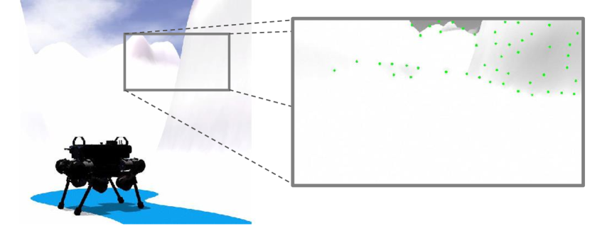
To prove the performance of STEP even in the extreme environments, we constructed the mountain terrain simulation world as shown in Fig.  3. We designed the overall simulation environment to be bright and texture-less so that it was challenging for visual-dependent approaches. Moreover, we included the experimental results on several slippery surfaces that made non-slip assumption invalid. The total distance traveled was approximately 200m.

Figure 3: ANYmal [19] on a slippery artifact in the simulation. The slippery surfaces are colored in blue. The right image in the gray box is obtained from the camera of ANYmal in white mountainous simulation environment in Gazebo. The point features tracked in VINS-Fusion [24] are marked with green dots.

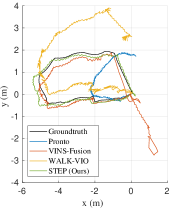
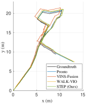
We implemented and evaluated several algorithms (see Table I). As expected, due to the limitation of loosely coupled approaches, Pronto [11] degraded if any sensor data is not stable. Therefore, Pronto showed a relatively large error in the texture-less and slippery environment.

Contrarily, the tightly coupled visual-inertial odometry system, VINS-Fusion [24] showed relatively better performance. However, WALK-VIO [15] degraded on the slippery terrain due to the non-slip assumption, as described in Fig.  4.

STEP outperformed others because it estimates the foot pose more precisely because it never depends on a non-slip assumption. Note that the foot pose and the body pose are tightly coupled. Fig. 4 and 4 illustrate the more reliable performance of STEP than the others in the simulation.

V-B Public Dataset Evaluation

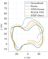
For legged robots, few public datasets are available. Thanks to the authors of [11], we evaluated STEP on the Fire Service College (FSC) dataset. The ANYmal [19] was utilized to acquire the FSC dataset. As described in Table I and Fig. 4, the leg kinematics-aided algorithm shows slightly better performance. All algorithms presented adequate performance because this dataset does not include light changes or severe slippages. This result also demonstrates that STEP can be considered an alternative to VINS-Fusion in the real world.

V-C Real-world Experiment

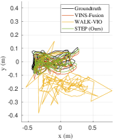
Mini-Cheetah [2] has been validated to run dynamically and aggressively. Thus, we favored it as our target platform. We conducted the experiment for approximately 2 minutes on gravel. The main purpose of this experiment was to show that the approaches based on non-slip assumption deteriorate under severe slippages. As described in Table I and Fig. 4, STEP shows the best performance although we evaluated STEP on uneven and slippery terrain, and VINS-Fusion shows comparable achievement due to many abundant textures from the environment. As expected, WALK-VIO deteriorated. Since the actual robot includes more severe noise and modeling uncertainty, the performance of the state estimator has been more degraded than the simulation results. Note that Pronto was not evaluated because the effects of preintegrated velocity factor were only focused on.

V-D Discussion

We show the effect of the preintegrated foot velocity factor by testing STEP in various environments. As can be seen in Table I, STEP showed a good performance even in the texture-less or slippery environments. We believe that this is because the preintegrated foot velocity factor helped improve foot pose estimation. Because the body pose is tightly coupled with the end effector pose, the body pose can also be estimated accurately. In contrast, WALK-VIO based on the non-slip assumption has a poor performance in the slippery environment. We conclude that it fails because adding only Gaussian noise could not compensate for the severe slippage effect, leading to inaccurately estimating the foot pose.

VI Conclusion and Future Works

This letter presents STEP, a novel method to deal with state estimation of legged robots in a general environment even under severe slippages. The preintegrated foot velocity factor plays an essential role in accurate state estimation. The robustness of STEP was validated in the slippery, and texture-less environment, in which the non-slip assumption is prone to be violated. Moreover, STEP was demonstrated using a public dataset and a real-legged robot. The results show that STEP can be considered a competitive estimator for the legged robot.

Further quantitative analysis of the preintegrated foot velocity factor, such as execution time and foot pose estimation accuracy, should be performed. In addition, a fusion of additional sensors, such as the LiDAR sensor, could be considered. One assumption we used in (28) could be critical when the robot has aggressive motion between consecutive keyframes. Thus, a more robust way to measure the body velocity has to be developed.

TABLE I: Translation ATE (Absolute trajectory error) and RPE (Relative pose error) over 1 $\mathrm{m}$ (RMSE, Unit: $\mathrm{m}$)

	Simulation (Gazebo)				Public dataset		Real robot platform
	Texture-less environment		Slippery environment		Fire Service College (FSC)		Mini-Cheetah on gravel
Traveled distance	$\approx 200\text{m}$		$\approx 15\text{m}$		$\approx 60\text{m}$		$\approx 15\text{m}$
	ATE	RPE	ATE	RPE	ATE	RPE	ATE	RPE
Pronto[11]	7.391	1.958	0.992	1.128	0.462	1.427	N.A	N.A
VINS-Fusion[24]	1.882	1.459	0.766	1.052	0.572	2.187	0.091	0.218
WALK-VIO[15]	1.701	1.454	0.682	1.188	0.518	1.867	0.313	0.461
STEP (Ours)	1.462	1.355	0.200	0.676	0.495	1.526	0.087	0.156

Figure 4: (a) The estimated trajectories of ANYmal in the simulation, especially in texture-less environment, and (b) in the slippery environment in the simulation, (c) in the FSC dataset, and (d) in the real-world experiment using Mini-Cheetah. All starting points are zero.

References

- [1] M. Bloesch, C. Gehring, P. Fankhauser, M. Hutter, M. A. Hoepflinger, and R. Siegwart, “State estimation for legged robots on unstable and slippery terrain,” in Proc. IEEE/RSJ International Conference on Intelligent Robots and Systems (IROS), 2013, pp. 6058–6064.
- [2] B. Katz, J. Di Carlo, and S. Kim, “Mini cheetah: A platform for pushing the limits of dynamic quadruped control,” in Proc. IEEE International Conference on Robotics and Automation (ICRA), 2019, pp. 6295–6301.
- [3] R. Hartley, M. Ghaffari, R. M. Eustice, and J. W. Grizzle, “Contact-aided invariant extended kalman filtering for robot state estimation,” The International Journal of Robotics Research, vol. 39, no. 4, pp. 402–430, 2020.
- [4] S. Teng, M. W. Mueller, and K. Sreenath, “Legged robot state estimation in slippery environments using invariant extended Kalman filter with velocity update,” arXiv preprint arXiv:2104.04238, 2021.
- [5] M. Fourmy, T. Flayols, N. Mansard, and J. Solà, “Contact forces pre-integration for the whole body estimation of legged robots,” in Proc. IEEE International Conference on Robotics and Automation (ICRA), 2021.
- [6] J.-H. Kim, S. Hong, G. Ji, S. Jeon, J. Hwangbo, J.-H. Oh, and H.-W. Park, “Legged robot state estimation with dynamic contact event information,” IEEE Robotics and Automation Letters, vol. 6, no. 4, pp. 6733–6740, 2021.
- [7] R. Hartley, J. Mangelson, L. Gan, M. G. Jadidi, J. M. Walls, R. M. Eustice, and J. W. Grizzle, “Legged robot state-estimation through combined forward kinematic and preintegrated contact factors,” in Proc. IEEE International Conference on Robotics and Automation (ICRA), 2018, pp. 4422–4429.
- [8] R. Hartley, M. G. Jadidi, L. Gan, J.-K. Huang, J. W. Grizzle, and R. M. Eustice, “Hybrid contact preintegration for visual-inertial-contact state estimation using factor graphs,” in Proc. IEEE/RSJ International Conference on Intelligent Robots and Systems (IROS), 2018, pp. 3783–3790.
- [9] A. Barrau, “Non-linear state error based extended kalman filters with applications to navigation,” Ph.D. dissertation, Mines Paristech, 2015.
- [10] C. Forster, L. Carlone, F. Dellaert, and D. Scaramuzza, “On-manifold preintegration for real-time visual–inertial odometry,” IEEE Transactions on Robotics, vol. 33, no. 1, pp. 1–21, 2016.
- [11] M. Camurri, M. Ramezani, S. Nobili, and M. Fallon, “Pronto: A multi-sensor state estimator for legged robots in real-world scenarios,” Frontiers in Robotics and AI, vol. 7, p. 68, 2020.
- [12] D. Wisth, M. Camurri, and M. Fallon, “Robust legged robot state estimation using factor graph optimization,” IEEE Robotics and Automation Letters, vol. 4, no. 4, pp. 4507–4514, 2019.
- [13] ——, “Preintegrated velocity bias estimation to overcome contact nonlinearities in legged robot odometry,” in Proc. IEEE International Conference on Robotics and Automation (ICRA), 2020, pp. 392–398.
- [14] ——, “VILENS: Visual, inertial, lidar, and leg odometry for all-terrain legged robots,” arXiv preprint arXiv:2107.07243, 2021.
- [15] H. Lim, B. Yu, Y. Kim, J. Byun, S. Kwon, H. Park, and H. Myung, “WALK-VIO: Walking-motion-adaptive leg kinematic constraint visual-inertial odometry for quadruped robots,” arXiv preprint arXiv:2111.15164, 2021.
- [16] J. Hwangbo, C. D. Bellicoso, P. Fankhauser, and M. Hutter, “Probabilistic foot contact estimation by fusing information from dynamics and differential/forward kinematics,” in Proc. IEEE/RSJ International Conference on Intelligent Robots and Systems (IROS), 2016, pp. 3872–3878.
- [17] M. Camurri, M. Fallon, S. Bazeille, A. Radulescu, V. Barasuol, D. G. Caldwell, and C. Semini, “Probabilistic contact estimation and impact detection for state estimation of quadruped robots,” IEEE Robotics and Automation Letters, vol. 2, no. 2, pp. 1023–1030, 2017.
- [18] F. Jenelten, J. Hwangbo, F. Tresoldi, C. D. Bellicoso, and M. Hutter, “Dynamic locomotion on slippery ground,” IEEE Robotics and Automation Letters, vol. 4, no. 4, pp. 4170–4176, 2019.
- [19] M. Hutter, C. Gehring, D. Jud, A. Lauber, C. D. Bellicoso, V. Tsounis, J. Hwangbo, K. Bodie, P. Fankhauser, M. Bloesch et al., “Anymal-a highly mobile and dynamic quadrupedal robot,” in Proc. IEEE/RSJ International Conference on Intelligent Robots and Systems (IROS), 2016, pp. 38–44.
- [20] G. S. Chirikjian, Stochastic Models, Information Theory, and Lie Groups, Volume 2: Analytic Methods and Modern Applications. Springer Science & Business Media, 2009, vol. 2.
- [21] P.-A. Absil, R. Mahony, and R. Sepulchre, Optimization Algorithms on Matrix Manifolds. Princeton University Press, 2009.
- [22] B. Hall, Lie Groups, Lie Algebras, and Representations: an Elementary Introduction. Springer, 2015, vol. 222.
- [23] T. D. Barfoot and P. T. Furgale, “Associating uncertainty with three-dimensional poses for use in estimation problems,” IEEE Transactions on Robotics, vol. 30, no. 3, pp. 679–693, 2014.
- [24] T. Qin, J. Pan, S. Cao, and S. Shen, “A general optimization-based framework for local odometry estimation with multiple sensors,” arXiv preprint arXiv:1901.03638, 2019.
- [25] P. J. Huber, “Robust estimation of a location parameter,” in Breakthroughs in Statistics. Springer, 1992, pp. 492–518.
- [26] J. J. Moré, “The Levenberg-Marquardt algorithm: implementation and theory,” Numerical Analysis, pp. 105–116, 1978.
- [27] W. Ci and Y. Huang, “A robust method for ego-motion estimation in urban environment using stereo camera,” Sensors, vol. 16, no. 10, p. 1704, 2016.
- [28] A. M. Andrew, “Multiple view geometry in computer vision,” Kybernetes, 2001.
- [29] R. Hartley, J. Mangelson, L. Gan, M. G. Jadidi, J. M. Walls, R. M. Eustice, and J. W. Grizzle, “Supplementary material: legged robot state-estimation through combined kinematic and preintegrated contact factors,” University of Michigan, Techsensoff. Rep., Feb, 2017.