Dynamics of charge-imbalance-resolved entanglement negativity after a quench in a free-fermion model

Abstract

The presence of a global internal symmetry in a quantum many-body system is reflected in the fact that the entanglement between its subparts is endowed with an internal structure, namely it can be decomposed as sum of contributions associated to each symmetry sector. The symmetry resolution of entanglement measures provides a formidable tool to probe the out-of-equilibrium dynamics of quantum systems. Here, we study the time evolution of charge-imbalance-resolved negativity after a global quench in the context of free-fermion systems, complementing former works for the symmetry-resolved entanglement entropy.

We find that the charge-imbalance-resolved logarithmic negativity shows an effective equipartition in the scaling limit of large times and system size, with a perfect equipartition for early and infinite times. We also derive and conjecture a formula for the dynamics of the charged Rényi logarithmic negativities. We argue that our results can be understood in the framework of the quasiparticle picture for the entanglement dynamics, and provide a conjecture that we expect to be valid for generic integrable models.

1 Introduction

The nonequilibrium dynamics of isolated quantum systems received considerable attention over the last two decades. In particular, the entanglement dynamics plays a fundamental role in our understanding of numerous aspects of quantum many-body systems out of equilibrium, such as the equilibration and thermalisation of isolated many-body systems [1, 2, 3, 4, 5], the emergence of thermodynamics in quantum systems [6, 7, 8, 9] or the effectiveness of classical computers to simulate quantum dynamics [10, 11, 12, 13, 14]. In one-dimensional quantum integrable systems, the entanglement dynamics after a quantum quench [15, 16, 17], the simplest and most broadly studied protocol to drive a quantum system out of equilibrium, is well described and understood in terms of the quasiparticle picture [15, 18, 19, 20]. These theoretical developments benefited from pioneering cold-atom and ion-trap experiments that could probe isolated quantum systems at large time scales with an unprecedented precision. Most notably, it has been possible to measure the entanglement of many-body systems out of equilibrium [21, 22, 23, 24].

For a bipartite quantum system in a pure state described by a density matrix $\rho$, the entanglement between a subsystem $A$ and its complement $B$ is quantified by the Rényi entropies

$$S_{n}\equiv\frac{1}{1-n}\log\text{Tr}\rho_{A}^{n},$$ (1.1)

where $\rho_{A}=\text{Tr}_{B}\rho$ is the reduced density matrix (RDM) of the subsystem $A$. In particular, the limit $n\to 1$ of the Rényi entropies yields the celebrated entanglement entropy

$$S_{1}\equiv\lim_{n\to 1}S_{n}=-\text{Tr}\rho_{A}\log\rho_{A}.$$ (1.2)

The Rényi entropies quantify the entanglement between a subsystem $A$ and its complement, irrespective of the topology of $A$. It is often relevant to consider the case where $A$ is itself a bipartite system $A=A_{1}\cup A_{2}$, and investigate the entanglement between $A_{1}$ and $A_{2}$. To this end, one usually introduces the Rényi mutual informations, defined as

$$I_{n}^{A_{1}:A_{2}}=S^{A_{1}}_{n}+S^{A_{2}}_{n}-S^{A_{1}\cup A_{2}}_{n}=\frac{1}{n-1}\log\left(\frac{\text{Tr}\rho_{A_{1}\cup A_{2}}^{n}}{\text{Tr}\rho_{A_{1}}^{n}\text{Tr}\rho_{A_{2}}^{n}}\right).$$ (1.3)

However, these quantities are not proper entanglement measures but rather quantify the global correlations between the two subsystems [25].

A suitable measure of entanglement between two non-complementary subsystems $A_{1}$ and $A_{2}$ is instead the entanglement negativity, defined as [26]

$$\mathcal{N}^{(b)}\equiv\frac{\text{Tr}|\rho_{A}^{T_{1}}|-1}{2},$$ (1.4)

where $\text{Tr}|O|=\text{Tr}\sqrt{O^{\dagger}O}$ is the trace norm of the operator $O$, and $\rho_{A}^{T_{1}}$ is the partially-transposed RDM of the system $A=A_{1}\cup A_{2}$. The latter is defined as follow. We denote the Hilbert spaces corresponding to each subsystem by $\mathcal{H}_{1}$ and $\mathcal{H}_{2}$, with respective bases $|e_{j}^{1}\rangle$ and $|e_{k}^{2}\rangle$. With this notation, $\rho_{A}$ reads

$$\rho_{A}=\sum_{ijkl}\langle e_{i}^{1},e_{j}^{2}|\rho_{A}|e_{k}^{1},e_{l}^{2}\rangle|e_{i}^{1},e_{j}^{2}\rangle\langle e_{k}^{1},e_{l}^{2}|,$$ (1.5)

and its partial transpose with respect to the degrees of freedom of subsystem $A_{1}$ is defined as

$$\rho_{A}^{T_{1}}\equiv\sum_{ijkl}\langle e_{k}^{1},e_{j}^{2}|\rho_{A}|e_{i}^{1},e_{l}^{2}\rangle|e_{i}^{1},e_{j}^{2}\rangle\langle e_{k}^{1},e_{l}^{2}|.$$ (1.6)

In terms of projectors on basis states, the partial transposition corresponds to the operation

$$\left(|e_{i}^{1},e_{j}^{2}\rangle\langle e_{k}^{1},e_{l}^{2}|\right)^{T_{1}}\equiv|e_{k}^{1},e_{j}^{2}\rangle\langle e_{i}^{1},e_{l}^{2}|.$$ (1.7)

The negativity is related to the existence of negative eigenvalues in the spectrum of the partially-transposed RDM. Indeed, writing $\text{Tr}|\rho_{A}^{T_{1}}|$ in terms of the eigenvalues $\lambda_{i}$ of $\rho_{A}^{T_{1}}$, we have

$$\mathrm{Tr}|\rho_{A}^{T_{1}}|=\sum_{i}|\lambda_{i}|=\sum_{\lambda_{i}>0}|\lambda_{i}|+\sum_{\lambda_{i}<0}|\lambda_{i}|=1+2\sum_{\lambda_{i}<0}|\lambda_{i}|,$$ (1.8)

and hence

$$\mathcal{N}^{(b)}=\sum_{\lambda_{i}<0}|\lambda_{i}|,$$ (1.9)

in agreement with Peres separability criterion [27, 28, 29]. We also introduce the logarithmic negativity as

$$\mathcal{E}^{(b)}=\log\text{Tr}|\rho_{A}^{T_{1}}|.$$ (1.10)

When the system $A_{1}\cup A_{2}$ is in a pure state, it satisfies $\mathcal{E}^{(b)}=S_{1/2}^{A_{1}}$ [26]. However, the experimental measure of the negativity in many-body systems is nowadays only possible by full quantum tomography. For this reason, a few protocols to measure the moments $\mathrm{Tr}(\rho_{A}^{T_{1}})^{n}$ of the partial transpose have been proposed [31, 32, 24, 30], leading to an actual measure in an ion-trap experiment [24, 30]. Some linear combinations of these moments provide sufficient conditions (known as $p_{n}$-PPT conditions) to witness entanglement in mixed states. Hence, it is very important to provide theoretical predictions not only for the negativity, but also for the moments of the partial transpose (also known as Rényi negativities, see below).

A very recent line of research concerns the understanding of the interplay between symmetries and entanglement out of equilibrium, as highlighted in a recent experiment [22]. In the case where the system has a global symmetry, the entanglement splits between the various symmetry sectors, and this symmetry resolution of entanglement attracted a lot of attention recently [35, 36, 37, 38, 39, 40, 41, 42, 43, 44, 45, 46, 47, 48, 49, 50, 51, 52, 53, 33, 34, 54, 55, 56, 57, 30, 58, 59, 60, 61, 62, 63, 64, 65, 66, 67, 68, 69, 70, 71, 72, 73, 74, 75]. Moreover, symmetry-resolved quantities have already been measured experimentally [56, 30]. In the context of non-complementary subsystems and mixed-states, the charge-imbalance-resolved negativity was defined in [38] and has since been investigated in several circumstances [54, 66, 67, 30]. It plays a crucial role in the detection of entanglement in mixes-state quantum many-body systems [30]. However, little results are available regarding its non-equilibrium dynamics [30]. In this paper, we fill this gap studying two quenches from homogeneous initial states in a free-fermion model. In particular, we interpret our results in terms of the quasiparticle picture for the entanglement dynamics, and generalise results for the Rényi negativities [76].

This paper is organised as follows. In Sec. 2 we introduce a definition of negativity for fermionic systems based on the partial time-reversal (TR) transformation of the RDM. We also discuss the charge-imbalance-resolved negativity and its expression in terms of Fourier transforms of the charged moments. We express these charged moments in terms of the two-point correlation matrix in the context of free fermions in Sec. 3. We also define the tight-biding model and the two initial states that we consider in this work. In Sec. 4, we present our analytical results and conjectures for the quench dynamics of the charged moments for both quenches under consideration. We compute the Fourier transforms of the charged moments in Sec. 5 and investigate the dynamics of the charge-imbalance-resolved negativity. Moreover, we argue that we recover known results for the dynamics of the total negativity from the charge-imbalance-resolved one. We interpret our results in terms of the quasiparticle picture for the entanglement dynamics in Sec. 6, and present our conclusions and outlooks in Sec. 7.

2 Negativity for fermionic systems and charge imbalance

In this section, we define the (fermionic) negativity and its charge-imbalance-resolved version in the context of fermionic systems with a global $U(1)$ symmetry.

2.1 Fermionic negativity

The definition of the negativity in Eq. (1.4) is not well-suited to investigate entanglement properties in the context of free-fermion systems. The main reason is that, for such systems, the partial transpose $\rho_{A}^{T_{1}}$, unlike $\rho_{A}$, is not a Gaussian operator, but rather a sum of two non-commuting Gaussian operators [77]. As a consequence, its full spectrum is not accessible [78, 79, 80]. To circumvent this issue, the partial TR transformation of the RDM, denoted $\rho_{A}^{R_{1}}$, has been introduced [81, 82, 83, 84, 85, 86, 87, 89, 88]. To define the partial TR transformation, let us consider the example of a single-state system described by fermionic operators $c$ and $c^{\dagger}$, with $\{c,c^{\dagger}\}=1$. In the basis of the fermionic coherent states $|\xi\rangle=\mathrm{e}^{-\xi c^{\dagger}}|0\rangle$ and $\langle\bar{\xi}|=\langle 0|\mathrm{e}^{-c\hskip 1.42271pt\bar{\xi}}$, where $\xi,\bar{\xi}$ are Grassmann variables, the TR transformation is defined as

$$(\ket{\xi}\bra{\bar{\xi}})^{R}\equiv\ket{\mathrm{i}\bar{\xi}}\bra{\mathrm{i}\xi}.$$ (2.1)

In particular, the TR transformation differs from the standard transposition by the presence of the factor $\mathrm{i}$. In the case of a many-particle system, the partial TR transformation on the degrees of freedom of subsystem $A_{1}$ is defined as

$$(\ket{\{\xi_{j}\}_{j\in A_{1}},\{\xi_{j}\}_{j\in A_{2}}}\bra{\{\bar{\chi}_{j}\}_{j\in A_{1}},\{\bar{\chi}_{j}\}_{j\in A_{2}}})^{R_{1}}\equiv\ket{\{\mathrm{i}\bar{\chi}_{j}\}_{j\in A_{1}},\{\xi_{j}\}_{j\in A_{2}}}\bra{\{\mathrm{i}\xi_{j}\}_{j\in A_{1}},\{\bar{\chi}_{j}\}_{j\in A_{2}}},$$ (2.2)

where $\ket{\{\xi_{j}\}}=\mathrm{e}^{-\sum_{j}\xi_{j}c^{\dagger}_{j}}\ket{0}$, $\bra{\{\bar{\chi}_{j}\}}=\bra{0}\mathrm{e}^{-\sum_{j}c_{j}\bar{\chi}_{j}}$ are the many-particle fermionic coherent states.

From $\rho_{A}^{R_{1}}$, one defines the fermionic negativity as

$$\mathcal{N}\equiv\frac{\mathrm{Tr}|\rho_{A}^{R_{1}}|-1}{2}=\frac{\mathrm{Tr}\sqrt{\rho_{A}^{R_{1}}(\rho_{A}^{R_{1}})^{\dagger}}-1}{2},$$ (2.3)

and the fermionic logarithmic negativity is

$$\mathcal{E}=\log\text{Tr}|\rho_{A}^{R_{1}}|.$$ (2.4)

It is possible to show that these fermionic negativities are entanglement monotones [84] and that they can capture some entanglement that is overlooked by the standard negativity. Since we only consider fermionic systems, we refer to these quantities as the negativity and the logarithmic negativity, respectively. In contrast, the quantities $\mathcal{N}^{(b)}$ and $\mathcal{E}^{(b)}$ in Eqs. (1.4) and (1.10) are sometimes referred to as bosonic negativity and bosonic logarithmic negativity, respectively. Contrarily to the bosonic negativity, the (fermionic) negativity is not related to the presence of negative eigenvalues in the spectrum of the partial TR transformed RDM, see [86].

We also introduce the Rényi (logarithmic) negativities as [86]

$$\mathcal{N}_{n}=\frac{N_{n}-1}{2},\qquad\mathcal{E}_{n}=\log N_{n},\qquad N_{n}=\begin{cases}\mathrm{Tr}\big{(}\rho_{A}^{R_{1}}(\rho_{A}^{R_{1}})^{\dagger}\dots\rho_{A}^{R_{1}}(\rho_{A}^{R_{1}})^{\dagger}\big{)},&\quad\mathrm{even}\ n,\\[5.69046pt] \mathrm{Tr}\big{(}\rho_{A}^{R_{1}}(\rho_{A}^{R_{1}})^{\dagger}\dots\rho_{A}^{R_{1}}\big{)},&\quad\mathrm{odd}\ n,\end{cases}$$ (2.5)

from which the negativity and logarithmic negativity are obtained in the replica limit $n_{e}\to 1$ with even $n_{e}$ [90, 91],

$$\mathcal{N}=\lim_{n_{e}\to 1}\mathcal{N}_{n_{e}},\quad\mathcal{E}=\lim_{n_{e}\to 1}\mathcal{E}_{n_{e}}.$$ (2.6)

We stress that the limit $\lim_{n_{e}\to 1}N_{n_{e}}=\mathrm{Tr}\sqrt{\rho_{A}^{R_{1}}(\rho_{A}^{R_{1}})^{\dagger}}$ is different from $N_{1}=\text{Tr}(\rho_{A}^{R_{1}})=1$.

2.2 Charge-imbalance resolution

We consider an extended quantum system with an internal $U(1)$ symmetry generated by a local charge $Q$. If the system is described by a density matrix $\rho$ that only acts non-trivially in an eigenspace of $Q$, we have $[\rho,Q]=0$. In the case of a bipartition in two complementary subsystems $A$ and $B$, by locality, the charge $Q$ splits as sum of operators that act on the local degrees of freedom of the two parts, $Q=Q_{A}+Q_{B}$. Hence, the trace over the degrees of freedom of subsystem $B$ in the commutation relation $[\rho,Q]=0$ yields $[\rho_{A},Q_{A}]=0$, i.e. $\rho_{A}$ has a block diagonal form with each block corresponding to an eigenvalue of $Q_{A}$.

In the case where the subsystem $A$ is itself partitioned into two complementary subsystems $A_{1}$ and $A_{2}$, we denote with $Q_{1}$ and $Q_{2}$ the corresponding charge operators. As shown in [38], the partial transpose with respect to the degrees of freedom of subsystem $A_{1}$ performed on the commutation relation $[\rho_{A},Q_{A}]=0$ gives $[\rho_{A}^{T_{1}},Q_{2}-Q_{1}^{T_{1}}]=0$, so that the partially-transposed RDM can be decomposed in blocks that correspond to the eigenvalues of the charge-imbalance operator $Q_{2}-Q_{1}^{T_{1}}$. As pointed out in [54], a similar relation holds for the partial TR transformation, namely

$$[\rho_{A}^{R_{1}},Q_{2}-Q_{1}^{R_{1}}]=0.$$ (2.7)

In the following, we define the operator $\hat{Q}_{A}\equiv Q_{2}-Q_{1}^{R_{1}}$ as the charge-imbalance operator, since we only deal with fermionic systems and partial TR transformation. We denote the eigenvalues of $\hat{Q}_{A}$ by $q$, and the projector on the corresponding eigenspace is $\Pi_{q}$. The charge-imbalance operator is basis-dependent (see, e.g., [54]), and reads $\hat{Q}_{A}=Q_{2}+Q_{1}-\ell/2$ in our computational basis, where $\ell$ is the length of the subsystem $A$, see [54]. From Eq. (2.7), we have the following decomposition of the partial TR transformed RDM,

$$\rho_{A}^{R_{1}}=\oplus_{q}p(q)\rho_{A}^{R_{1}}(q),$$ (2.8)

where $p(q)=\mathrm{Tr}(\Pi_{q}\rho_{A}^{R_{1}})$ is the probability of finding $q$ as the outcome of a measurement of $\hat{Q}_{A}$. The operator $\rho_{A}^{R_{1}}(q)$ is the charge-imbalance-resolved partial TR transformed RDM, defined as

$$\rho_{A}^{R_{1}}(q)=\frac{\Pi_{q}\rho_{A}^{R_{1}}\Pi_{q}}{\mathrm{Tr}(\Pi_{q}\rho_{A}^{R_{1}})},\qquad\mathrm{Tr}(\rho_{A}^{R_{1}}(q))=1.$$ (2.9)

The charge-imbalance-resolved negativity is defined as

$$\mathcal{N}(q)=\frac{\mathrm{Tr}|\rho_{A}^{R_{1}}(q)|-1}{2},\qquad$$ (2.10)

and satisfies

$$\mathcal{N}=\sum_{q}p(q)\mathcal{N}(q).$$ (2.11)

Here we also define a charge-imbalance-resolved logarithmic negativity as

$$\hat{\mathcal{E}}(q)=\log\mathrm{Tr}|\rho_{A}^{R_{1}}(q)|=\log(2\mathcal{N}(q)+1)\,.$$ (2.12)

However, because of the non-linearity of the logarithm, $\hat{\mathcal{E}}(q)$ does not represent a proper resolution (in the sense that it is not the contribution of the sector $q$ to the total logarithmic negativity), but it is a useful auxiliary quantity related to ${\mathcal{N}}(q)$.

It is also useful to define the charge-imbalance-resolved Rényi negativities

$$\mathcal{N}_{n}(q)=\frac{\hat{N}_{n}(q)-1}{2},\qquad\hat{N}_{n}(q)=\begin{cases}\mathrm{Tr}\big{(}\rho_{A}^{R_{1}}(q)(\rho_{A}^{R_{1}}(q))^{\dagger}\dots\rho_{A}^{R_{1}}(q)(\rho_{A}^{R_{1}}(q))^{\dagger}\big{)},&\quad\mathrm{even}\ n,\\[5.69046pt] \mathrm{Tr}\big{(}\rho_{A}^{R_{1}}(q)(\rho_{A}^{R_{1}}(q))^{\dagger}\dots\rho_{A}^{R_{1}}(q)\big{)},&\quad\mathrm{odd}\ n,\end{cases}$$ (2.13)

and we have $\displaystyle\mathcal{N}(q)=\lim_{n_{e}\to 1}\mathcal{N}_{n_{e}}(q)$.

To compute these quantities, the method developped in [38] is similar to the case of the symmetry-resolved entropies [36], where one introduces the charged moments [92, 93, 94] and investigates their Fourier transforms. To proceed, we introduce the charged Rényi logarithmic negativities [54]

$$\mathcal{E}_{n}(\alpha)=\log N_{n}(\alpha),\qquad N_{n}(\alpha)=\begin{cases}\mathrm{Tr}(\rho_{A}^{R_{1}}(\rho_{A}^{R_{1}})^{\dagger}\dots\rho_{A}^{R_{1}}(\rho_{A}^{R_{1}})^{\dagger}\mathrm{e}^{\mathrm{i}\hat{Q}_{A}\alpha}),&\quad\mathrm{even}\ n,\\ \mathrm{Tr}(\rho_{A}^{R_{1}}(\rho_{A}^{R_{1}})^{\dagger}\dots\rho_{A}^{R_{1}}\mathrm{e}^{\mathrm{i}\hat{Q}_{A}\alpha}),&\quad\mathrm{odd}\ n,\end{cases}$$ (2.14)

where the quantities $N_{n}(\alpha)$ are the charged moments. The limit $n_{e}\to 1$ defines the charged logarithmic negativity

$$\mathcal{E}(\alpha)\equiv\lim_{n_{e}\to 1}\log N_{n_{e}}(\alpha),$$ (2.15)

and we call the moment $N_{1}(\alpha)=\text{Tr}[\rho_{A}^{R_{1}}\mathrm{e}^{\mathrm{i}\hat{Q}_{A}\alpha}]$ the charged probability, since its Fourier transform gives the probability $p(q)$.

The Fourier transforms of the charged moments yield the charge-imbalance-resolved negativities [54],

$$\mathcal{Z}_{R_{1},n}(q)=\displaystyle\int_{-\pi}^{\pi}\frac{d\alpha}{2\pi}\mathrm{e}^{-\mathrm{i}q\alpha}N_{n}(\alpha),\quad p(q)=\displaystyle\int_{-\pi}^{\pi}\frac{d\alpha}{2\pi}\mathrm{e}^{-\mathrm{i}q\alpha}N_{1}(\alpha),$$ (2.16)

from which

$$\hat{N}_{n}(q)=\frac{\mathcal{Z}_{R_{1},n}(q)}{p(q)^{n}}.$$ (2.17)

We also introduce the quantity

$$\mathcal{Z}_{R_{1}}(q)\equiv\lim_{n_{e}\to 1}\mathcal{Z}_{R_{1},n_{e}}(q)=\int_{-\pi}^{\pi}\frac{d\alpha}{2\pi}\mathrm{e}^{-\mathrm{i}q\alpha}\mathrm{e}^{\mathcal{E}(\alpha)},$$ (2.18)

and express the charge-imbalance-resolved (logarithmic) negativity as

$$\mathcal{N}(q)=\frac{1}{2}\Big{(}\frac{\mathcal{Z}_{R_{1}}(q)}{p(q)}-1\Big{)},\qquad\hat{\mathcal{E}}(q)=\log\Big{(}\frac{\mathcal{Z}_{R_{1}}(q)}{p(q)}\Big{)}.$$ (2.19)

3 Charged moments for free fermions

In this section, we introduce our quench protocol, i.e. the two initial states we consider and the free-fermion model that governs the time evolution. We also provide exact formulas for the charged moments in terms of the two-point correlation matrix.

3.1 Model and initial states

Figure 1: Illustration of the geometry we consider in the limit where the system size $L$ is very large. The system $A=A_{1}\cup A_{2}$ is in blue, whereas the system $B$ consists of the red regions.

In the following, we study the time evolution of the charged moments and the charge-imbalance-resolved negativity after a global quench in the tight-binding model with Hamiltonian

$$H=\sum_{j=1}^{L}(c_{j}^{\dagger}c_{j+1}+c_{j+1}^{\dagger}c_{j}).$$ (3.1)

Here, $c_{j}$ and $c_{j}^{\dagger}$ are the canonical fermionic annihilation and creation operators on site $j$. They satisfy the anticommutation relations $\{c_{i},c_{j}^{\dagger}\}=\delta_{i,j}$ and $\{c_{i},c_{j}\}=\{c_{i}^{\dagger},c_{j}^{\dagger}\}=0$. The system size is $L$, and we consider a chain with periodic boundary conditions. For simplicity, we assume that $L$ is even. The conserved charge is the fermion-number operator

$$Q=\sum\limits_{j=1}^{L}c_{j}^{\dagger}c_{j}.$$ (3.2)

In the chain, we consider a bipartition $A\cup B$ where $A$ consists of two intervals $A_{1}$ and $A_{2}$ separated by $d$ lattice sites, of respective lengths $\ell_{1}$ and $\ell_{2}$, with $\ell_{1}+\ell_{2}=\ell$. We illustrate this geometry in Fig. 1. For simplicity, we also assume that $d,\ell_{1},\ell_{2}$ are even numbers. The global conserved charge $Q$ trivially splits as a sum over $A_{1}$, $A_{2}$ and $B$,

$$Q=\sum_{j\in A_{1}}c_{j}^{\dagger}c_{j}+\sum_{j\in A_{2}}c_{j}^{\dagger}c_{j}+\sum_{j\in B}c_{j}^{\dagger}c_{j}\equiv Q_{1}+Q_{2}+Q_{B}.$$ (3.3)

We consider two simple homogeneous initial states, namely the Néel and the dimer states:

$$\begin{split}|N\rangle&=\prod_{j=1}^{L/2}c_{2j}^{\dagger}|0\rangle,\\ |D\rangle&=\prod_{j=1}^{L/2}\frac{c_{2j}^{\dagger}-c_{2j-1}^{\dagger}}{\sqrt{2}}|0\rangle.\end{split}$$ (3.4)

These two states enjoy important properties. First, the time-dependent density matrix

$$\rho(t)=\mathrm{e}^{-\mathrm{i}tH}|\psi_{0}\rangle\langle\psi_{0}|\mathrm{e}^{\mathrm{i}tH},\qquad|\psi_{0}\rangle=|N\rangle,|D\rangle,$$ (3.5)

where $H$ is the tight-biding Hamiltonian (3.1), commutes with the total charge $Q$ in Eq. (3.2) and is a Gaussian operator for all values of $t$. Second, their time-dependent correlation matrix

$$[C(t)]_{x,x^{\prime}}=\langle\psi_{0}|\mathrm{e}^{\mathrm{i}tH}c_{x}^{\dagger}c_{x^{\prime}}\mathrm{e}^{-\mathrm{i}tH}|\psi_{0}\rangle,\qquad|\psi_{0}\rangle=|N\rangle,|D\rangle,$$ (3.6)

is exactly known. For the quench from the Néel state, we have [95]

$$[C(t)]_{x,x^{\prime}}=\frac{\delta_{x,x^{\prime}}}{2}+\frac{(-1)^{x^{\prime}}}{2}\int_{-\pi}^{\pi}\frac{\mathrm{d}k}{2\pi}\mathrm{e}^{\mathrm{i}k(x-x^{\prime})+4\mathrm{i}t\cos k}.$$ (3.7)

For the dimer state, it reads [96]

$$[C(t)]_{j,k}=\Big{\langle}\begin{pmatrix}c_{2j-1}^{\dagger}\\ c_{2j}^{\dagger}\end{pmatrix}\begin{pmatrix}c_{2k-1}&c_{2k}\end{pmatrix}\Big{\rangle}=\frac{1}{2}\big{(}\delta_{j,k}\mathbb{I}_{2}+\Pi_{k-j}\big{)}$$ (3.8a)

where $$\Pi_{m}$$ is

$$\Pi_{m}=\int_{-\pi}^{\pi}\frac{\mathrm{d}k}{2\pi}\mathrm{e}^{-2\mathrm{i}mk}\ \begin{pmatrix}-f(k,t)&-g(k,t)\\ -g(k,t)^{*}&f(k,t)\\ \end{pmatrix}$$ (3.8b)

with

$$\begin{split}f(k,t)&=\sin k\sin(4\cos(k)t),\\ g(k,t)&=\mathrm{e}^{-\mathrm{i}k}(\cos k+\mathrm{i}\sin k\cos(4\cos(k)t)).\end{split}$$ (3.8c)

We stress that the Néel and dimer states are not the only states that satisfy these properties, but we focus on them for their simplicity.

3.2 Charged moments from correlation matrices

For the two quenches we consider, the RDM of $A$ is a Gaussian operator and can be obtained from the correlations matrix $C_{A}(t)=[C(t)]_{x,x^{\prime}}$ with $x,x^{\prime}\in A$ [97, 98, 99]. We introduce the matrix $J_{A_{1}\cup A_{2}}=2C_{A}-\mathbb{I}$ and denote its eigenvalues by $\nu_{j}$. Because of the geometry of $A$, $J_{A_{1}\cup A_{2}}$ has the following block structure,

$$J_{A_{1}\cup A_{2}}=\begin{pmatrix}J_{11}&J_{12}\\ J_{21}&J_{22}\end{pmatrix},$$ (3.9)

where $J_{ij}$ is a matrix of size $\ell_{i}\times\ell_{j}$ which contains the correlations between sites in $A_{i}$ and $A_{j}$. The exact form for the entries are given in Eqs. (3.7) and (3.8) for the quench from the Néel and the dimer state, respectively. From this matrix we introduce $J_{\pm}$ and $J_{\mathrm{x}}$, with respective eigenvalues $\nu^{\pm}_{j}$ and $\nu^{\mathrm{x}}_{j}$, as follows,

$$J_{\pm}=\begin{pmatrix}-J_{11}&\pm\mathrm{i}J_{12}\\ \pm\mathrm{i}J_{21}&J_{22}\end{pmatrix},$$ (3.10a)

and

$$J_{\mathrm{x}}=(\mathbb{I}+J_{+}J_{-})^{-1}\cdot(J_{+}+J_{-}).$$ (3.10b)

Following Refs. [38, 54, 84, 86, 100], we recover the formula for the charged moments $N_{n_{e}}(\alpha)$ with even $n_{e}$ defined in Eq. (2.14),

$$\log N_{n_{e}}(\alpha)=-\mathrm{i}\frac{\ell\alpha}{2}+\sum_{j=1}^{\ell}\log\Big{[}\Big{(}\frac{1+\nu^{\mathrm{x}}_{j}}{2}\Big{)}^{\frac{n_{e}}{2}}\mathrm{e}^{\mathrm{i}\alpha}+\Big{(}\frac{1-\nu^{\mathrm{x}}_{j}}{2}\Big{)}^{\frac{n_{e}}{2}}\Big{]}+\frac{n_{e}}{2}\sum_{j=1}^{\ell}\log\Big{[}\Big{(}\frac{1+\nu_{j}}{2}\Big{)}^{2}+\Big{(}\frac{1-\nu_{j}}{2}\Big{)}^{2}\Big{]}.$$ (3.11)

The limit for $n_{e}\rightarrow 1$ gives the charged logarithmic negativity,

$$\mathcal{E}(\alpha)=-\mathrm{i}\frac{\ell\alpha}{2}+\sum_{j=1}^{\ell}\log\Big{[}\Big{(}\frac{1+\nu^{\mathrm{x}}_{j}}{2}\Big{)}^{1/2}\mathrm{e}^{\mathrm{i}\alpha}+\Big{(}\frac{1-\nu^{\mathrm{x}}_{j}}{2}\Big{)}^{1/2}\Big{]}+\frac{1}{2}\sum_{j=1}^{\ell}\log\Big{[}\Big{(}\frac{1+\nu_{j}}{2}\Big{)}^{2}+\Big{(}\frac{1-\nu_{j}}{2}\Big{)}^{2}\Big{]}.$$ (3.12)

For odd $n_{o}$, we introduce two additional matrices,

$$J_{n_{o}}=\Big{[}(\mathbb{I}+J_{\mathrm{x}})^{\frac{n_{o}-1}{2}}+(\mathbb{I}-J_{\mathrm{x}})^{\frac{n_{o}-1}{2}}\Big{]}^{-1}\cdot\Big{[}(\mathbb{I}+J_{\mathrm{x}})^{\frac{n_{o}-1}{2}}-(\mathbb{I}-J_{\mathrm{x}})^{\frac{n_{o}-1}{2}}\Big{]},\\$$ (3.13a)

and

$$J_{\alpha}=\Big{[}\mathbb{I}+\frac{\mathrm{e}^{\mathrm{i}\alpha}-1}{\mathrm{e}^{\mathrm{i}\alpha}+1}J_{+}\Big{]}^{-1}\cdot\Big{[}J_{+}+\frac{\mathrm{e}^{\mathrm{i}\alpha}-1}{\mathrm{e}^{\mathrm{i}\alpha}+1}\mathbb{I}\Big{]},$$ (3.13b)

and find the expression

$$\log N_{n_{o}}(\alpha)=-\mathrm{i}\frac{\ell\alpha}{2}+\sum_{j=1}^{\ell}\log\Big{[}\frac{1+\nu^{+}_{j}}{2}\mathrm{e}^{\mathrm{i}\alpha}+\frac{1-\nu^{+}_{j}}{2}\Big{]}+\log\Big{[}\det\Big{(}\frac{\mathbb{I}+J_{n_{o}}\cdot J_{\alpha}}{2}\Big{)}\Big{]}\\ +\sum_{j=1}^{\ell}\log\Big{[}\Big{(}\frac{1+\nu^{\mathrm{x}}_{j}}{2}\Big{)}^{\frac{n_{o}-1}{2}}+\Big{(}\frac{1-\nu^{\mathrm{x}}_{j}}{2}\Big{)}^{\frac{n_{o}-1}{2}}\Big{]}+\frac{n_{o}-1}{2}\sum_{j=1}^{\ell}\log\Big{[}\Big{(}\frac{1+\nu_{j}}{2}\Big{)}^{2}+\Big{(}\frac{1-\nu_{j}}{2}\Big{)}^{2}\Big{]}.$$ (3.14)

Even though we used standard techniques from the algebra of Gaussian operators to derive this formula for odd values of $n_{o}$, it is, to the best of our knowledge, the first time it appears in the literature. The limit $n_{o}\to 1$ yields the known result from [54] for the charged probability $N_{1}(\alpha)$,

$$\log N_{1}(\alpha)=-\mathrm{i}\frac{\ell\alpha}{2}+\sum_{j=1}^{\ell}\log\Big{[}\frac{1+\nu^{+}_{j}}{2}\mathrm{e}^{\mathrm{i}\alpha}+\frac{1-\nu^{+}_{j}}{2}\Big{]}.$$ (3.15)

4 Quench dynamics of the charged Rényi logarithmic negativities

In this section, we present our analytical results and conjectures for the charged Rényi logarithmic negativities $\mathcal{E}_{n}(\alpha)=\log N_{n}(\alpha)$ after the quenches from the Néel and dimer states. The starting point in the computations is the exact expression for the two-point correlation matrix given in Eqs. (3.7) and (3.8) for the respective quenches.

4.1 Analytical results for $\boldsymbol{\mathcal{E}_{1}(\alpha)}$

To perform analytical calculations, it is useful to express the charged probability $N_{1}(\alpha)$ in (3.15) as a Taylor series in $\text{Tr}J_{+}^{m}$, where $J_{+}$ is defined in Eq. (3.10a). We introduce the function $h_{n,\alpha}(x)$ and the coefficients $c_{n,\alpha}(m)$ as

$$h_{n,\alpha}(x)=\log\left[\left(\frac{1+x}{2}\right)^{n}\mathrm{e}^{\mathrm{i}\alpha}+\left(\frac{1-x}{2}\right)^{n}\right]\equiv\sum_{m=0}^{\infty}c_{n,\alpha}(m)x^{m}$$ (4.1)

and conclude

$$\log N_{1}(\alpha)=-\mathrm{i}\frac{\ell\alpha}{2}+\sum_{m=0}^{\infty}c_{1,\alpha}(m)\text{Tr}J_{+}^{m}.$$ (4.2)

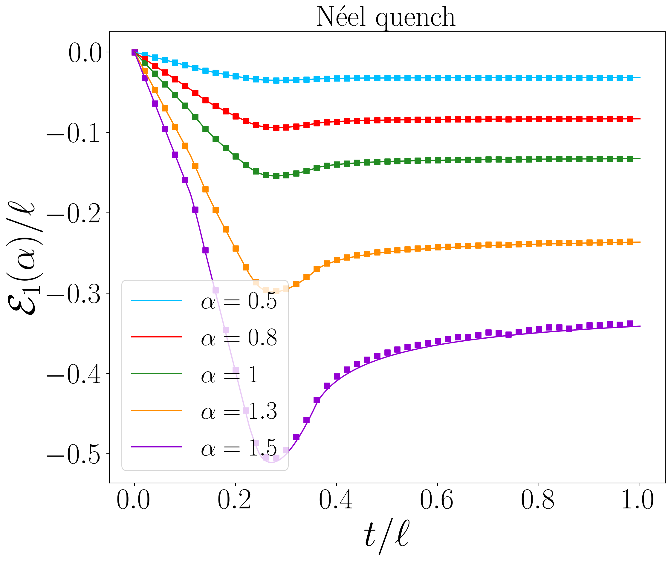
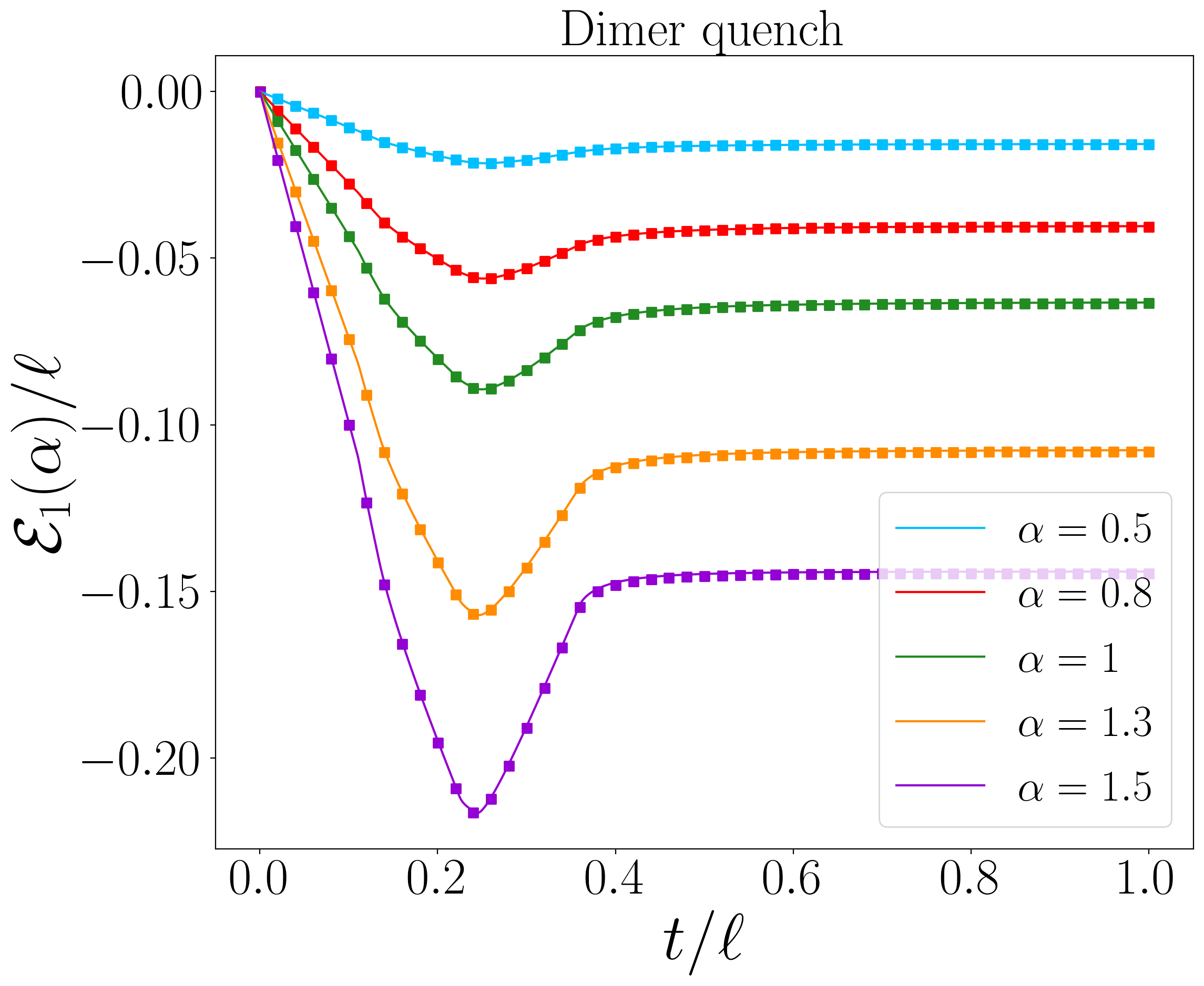
Figure 2: Time evolution of $\mathcal{E}_{1}(\alpha)$ after a quench from the Néel state (left) and the dimer state (right) in the tight-biding model (3.1) as a function of $t/\ell$ with $\ell_{1}=230$, $\ell_{2}=270$ and $d=220$. The analytical prediction of Eq. (4.6) (solid lines) perfectly matches the numerical data (symbols).

We use the stationary phase approximation discussed in [101] and generalise the procedure to the case where the subsystem $A$ consists of two disjoint intervals in the scaling limit where $\ell_{1},\ell_{2},d,t\to\infty$ with fixed ratios $\ell_{1}/\ell$, $d/\ell$ and $t/\ell$. This non-trivial extension of [101] allows us to derive new analytical results in the context of non-equilibrium disjoint systems, and in particular we find [102]

$$\begin{split}\text{Tr}J_{+}(t)^{2j}&=\ell-\int\frac{\mathrm{d}k}{2\pi}(1-x_{k}^{2j})(\min(\ell_{1},2v_{k}t)+\min(\ell_{2},2v_{k}t))\\ &+\int\frac{\mathrm{d}k}{2\pi}\sigma(x_{k},j)(\max(d,2v_{k}t)+\max(d+\ell,2v_{k}t)-\max(d+\ell_{1},2v_{k}t)-\max(d+\ell_{2},2v_{k}t)),\\ \text{Tr}J_{+}(t)^{2j+1}&=0,\end{split}$$ (4.3)

where

$$\sigma(x_{k},j)=\sum_{s=1}^{j}\sum_{t=0}^{2j-2s}(-1)^{s}x_{k}^{2j-2s}(1-x_{k}^{2})^{s}\frac{sj}{(2j-s-t)(s+t)}\begin{pmatrix}2j-s-t\\ s\end{pmatrix}\begin{pmatrix}s+t\\ s\end{pmatrix},$$ (4.4)

and $v_{k}=2|\sin k|$. The maximal value of the velocity is $v_{\max}=\max_{k}v_{k}=2$. The variable $x_{k}$ depends on the quench, and we have

$$x_{k}=\begin{cases}0,&\textrm{N\'{e}el},\\ \cos k,&\textrm{dimer}.\end{cases}$$ (4.5)

For the Néel case, there is an important simplification, since $\sigma(0,j)=(-1)^{j}$. The re-summation of (4.3) into Eq. (4.2) yields

$$\mathcal{E}_{1}(\alpha)=\int\frac{\mathrm{d}k}{2\pi}\mathrm{Re}[h_{1,\alpha}(x_{k})](\min(\ell_{1},2v_{k}t)+\min(\ell_{2},2v_{k}t))\\ -\int\frac{\mathrm{d}k}{2\pi}\mathrm{Re}[h_{1,\alpha}(x_{k})-\frac{1}{2}h_{1,2\alpha}(x_{k})](\max(d,2v_{k}t)+\max(d+\ell,2v_{k}t)-\max(d+\ell_{1},2v_{k}t)-\max(d+\ell_{2},2v_{k}t)).$$ (4.6)

We compare this analytical prediction with numerical results in Fig. 2 and find a very good agreement for both quenches.

4.2 Conjectures for $\boldsymbol{\mathcal{E}_{n}(\alpha)}$ with arbitrary $\boldsymbol{n}$

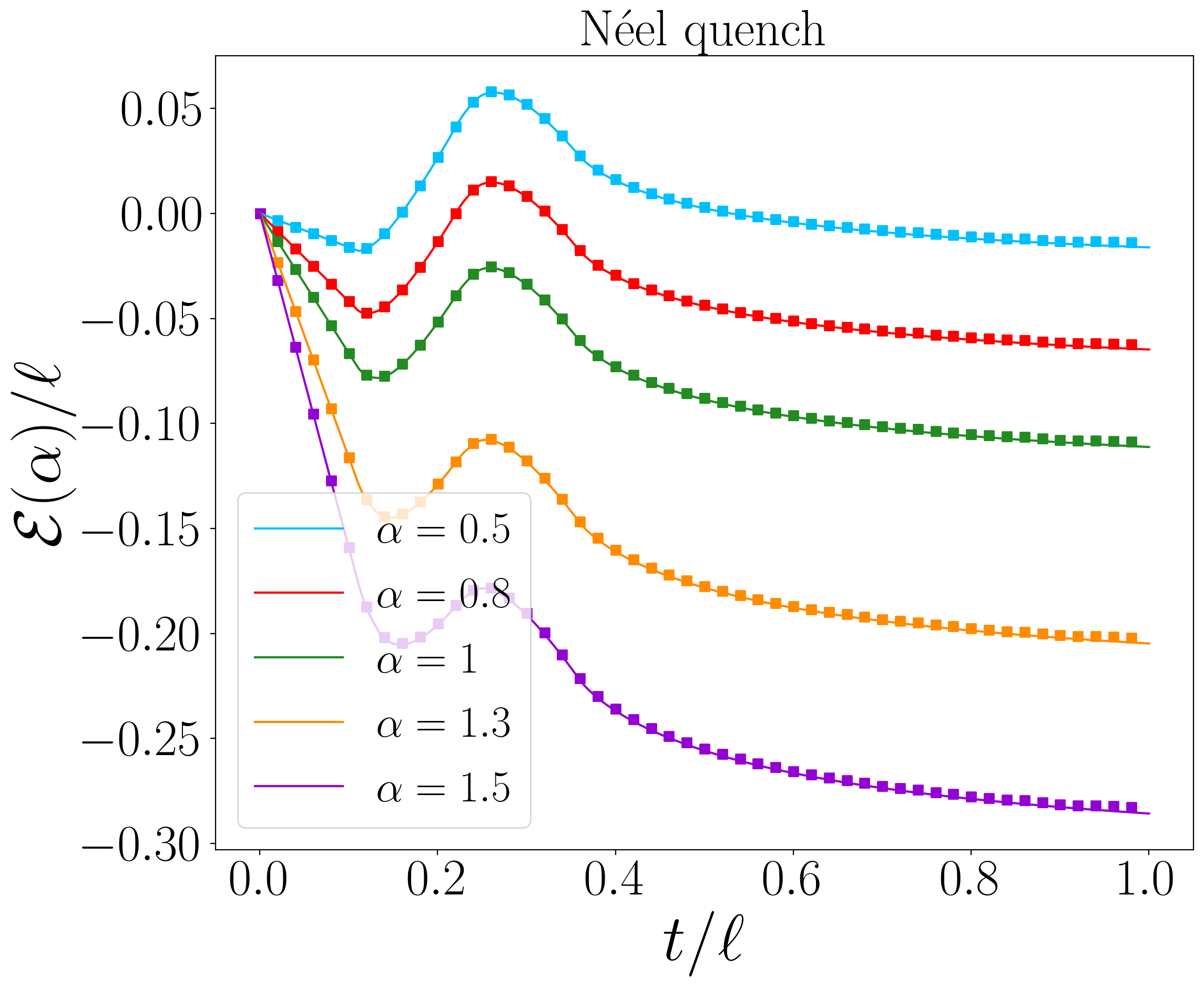
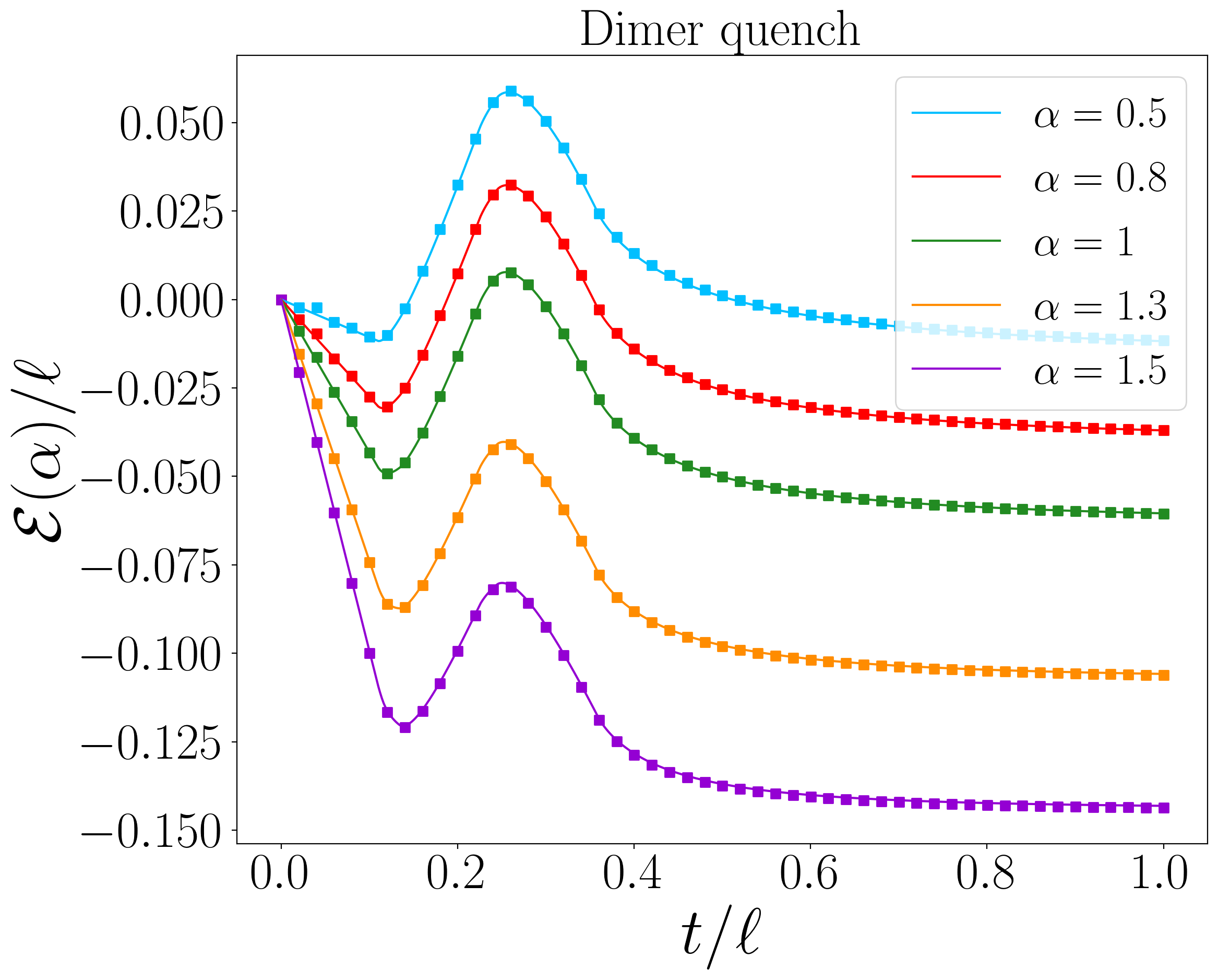
Figure 3: Time evolution of $\mathcal{E}(\alpha)$ after a quench from the Néel state (left) and the dimer state (right) in the tight-biding model (3.1) as a function of $t/\ell$ with $\ell_{1}=230$, $\ell_{2}=270$ and $d=220$. The conjecture of Eq. (4.9) (solid lines) perfectly matches the numerical data (symbols).

In the cases where $n\neq 1$, we conjecture

$$\mathcal{E}_{n}(\alpha)=\int\frac{\mathrm{d}k}{2\pi}\mathrm{Re}[h_{n,\alpha}(x_{k})](\min(\ell_{1},2v_{k}t)+\min(\ell_{2},2v_{k}t))\\ -\int\frac{\mathrm{d}k}{2\pi}\mathrm{Re}[h_{n,\alpha}(x_{k})-h^{(2)}_{n,\alpha}(x_{k})](\max(d,2v_{k}t)+\max(d+\ell,2v_{k}t)-\max(d+\ell_{1},2v_{k}t)-\max(d+\ell_{2},2v_{k}t))$$ (4.7)

with

$$h^{(2)}_{n,\alpha}(x_{k})=\begin{cases}\frac{1}{2}h_{n,2\alpha}(x_{k}),&\mathrm{odd}\ n,\\[8.5359pt] h_{\frac{n}{2},\alpha}(x_{k}),&\mathrm{even}\ n.\end{cases}$$ (4.8)

This formula reduces to the exact result (4.6) for $n=1$, and matches quasiparticle conjectures for the Rényi logarithmic negativities in the limit $\alpha=0$ [76]. In particular, for the charged logarithmic negativity, the limit $n_{e}\to 1$ in the even case yields

$$\mathcal{E}(\alpha)=\int\frac{\mathrm{d}k}{2\pi}\mathrm{Re}[h_{1,\alpha}(x_{k})](\min(\ell_{1},2v_{k}t)+\min(\ell_{2},2v_{k}t))\\ -\int\frac{\mathrm{d}k}{2\pi}\mathrm{Re}[h_{1,\alpha}(x_{k})-h_{1/2,\alpha}(x_{k})](\max(d,2v_{k}t)+\max(d+\ell,2v_{k}t)-\max(d+\ell_{1},2v_{k}t)-\max(d+\ell_{2},2v_{k}t)).$$ (4.9)

We compare the conjectures for the charged logarithmic negativity and $\mathcal{E}_{n}(\alpha)$ for even and odd $n$ in Figs. 3, 4 and 5, respectively. We systematically find a very good agreement between the conjectures (4.7), (4.9), and the numerical results, for both quenches.

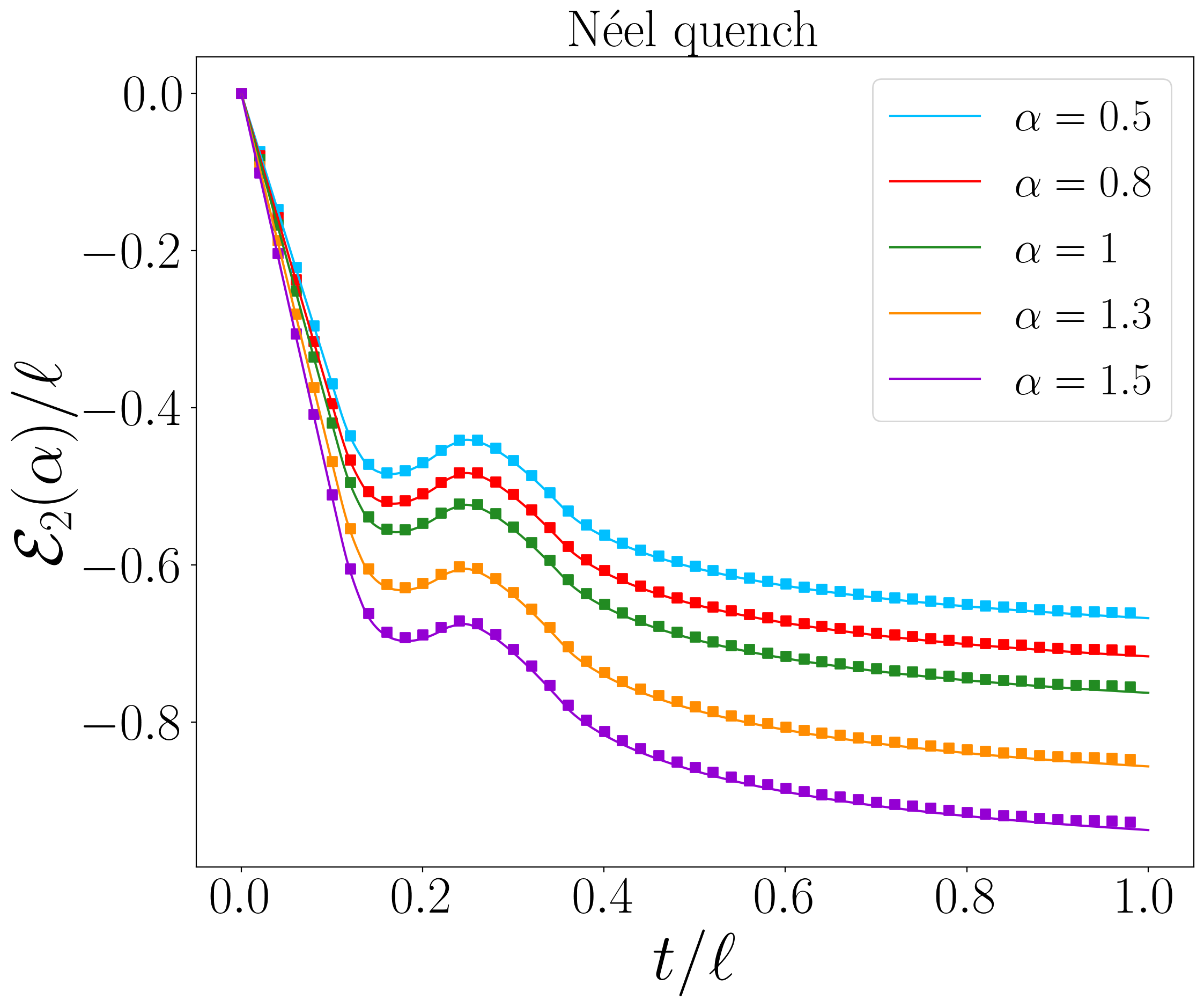
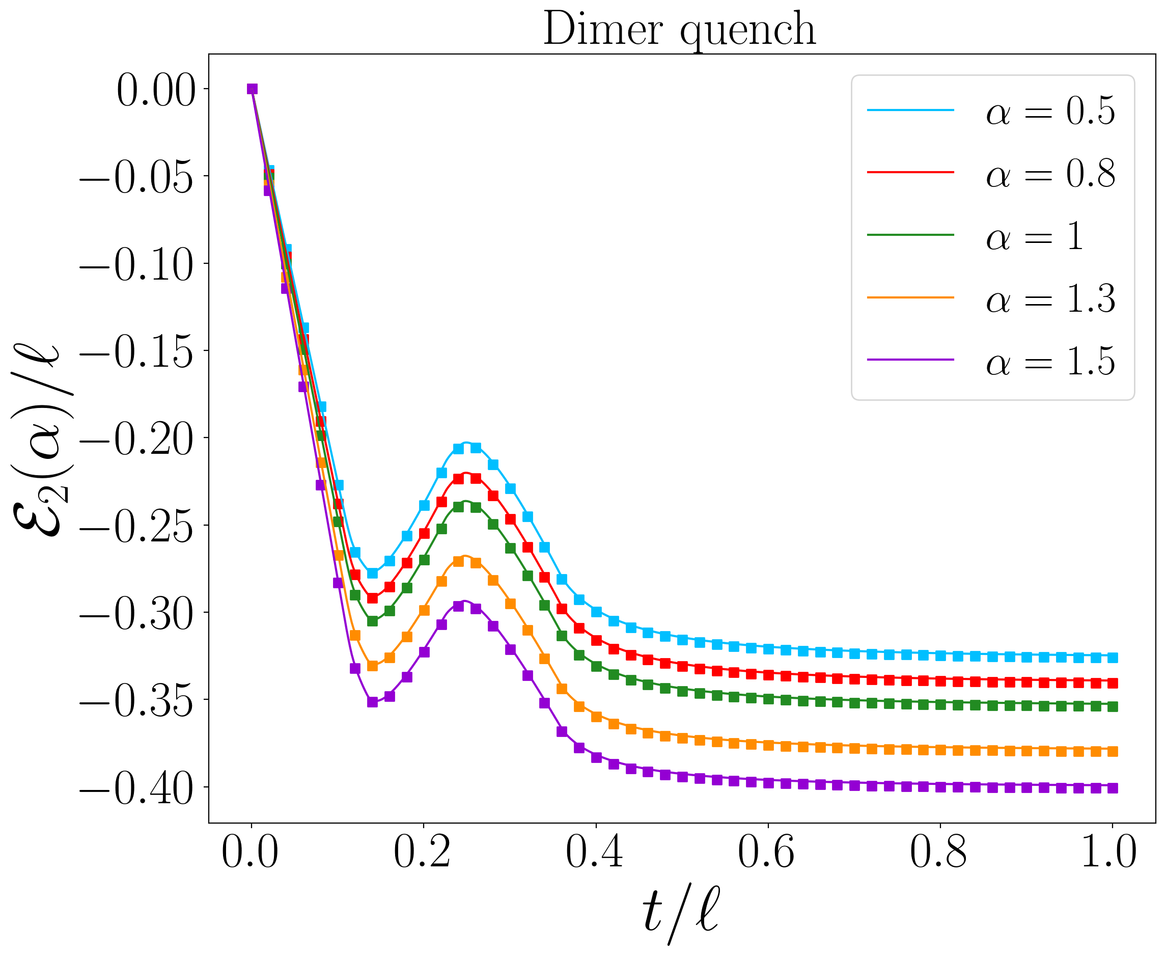
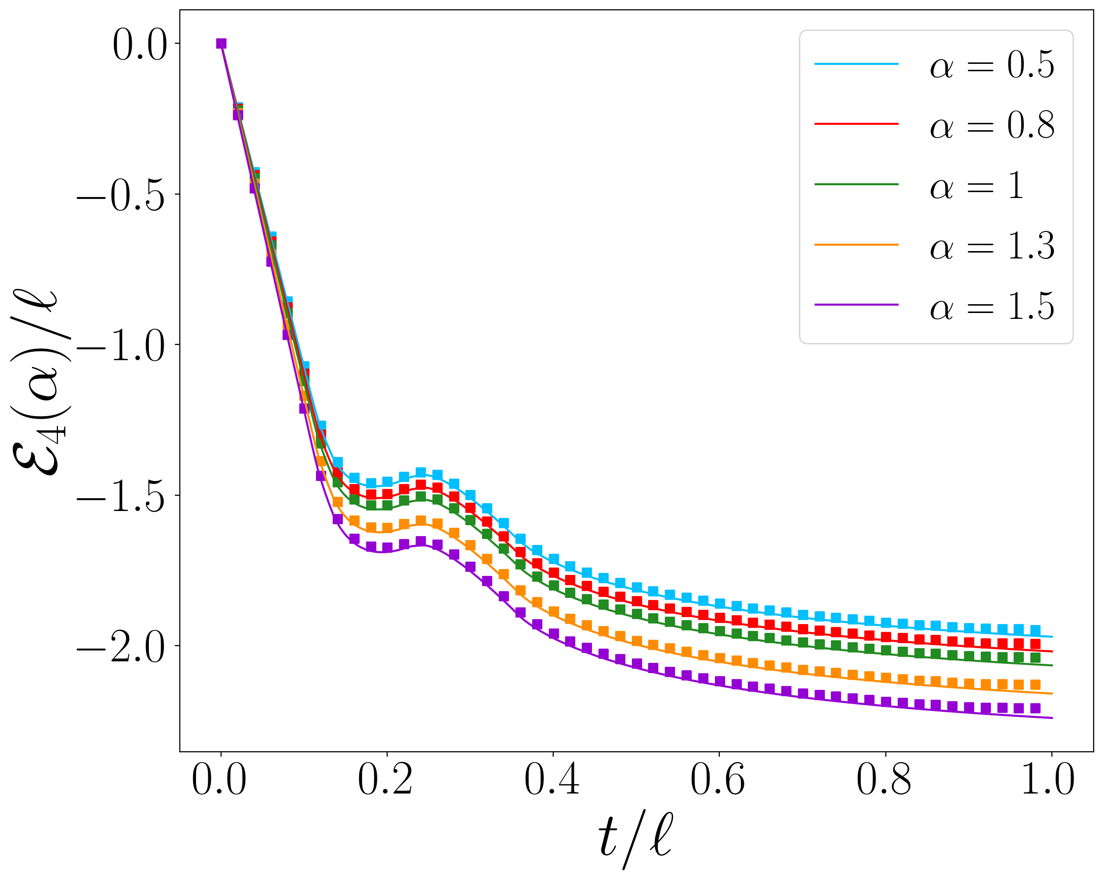
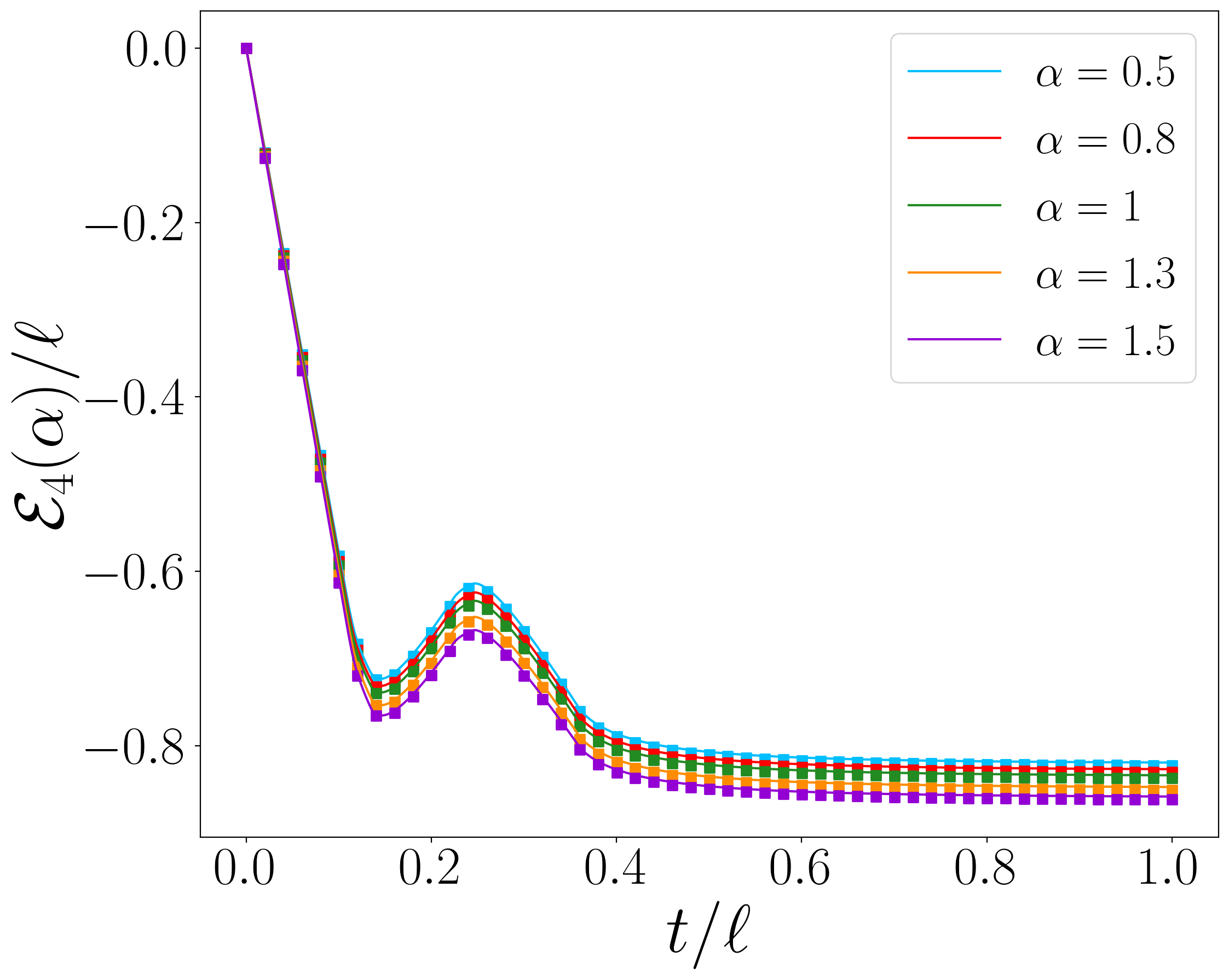
Figure 4: Time evolution of $\mathcal{E}_{n_{e}}(\alpha)$ with $n_{e}=2,4$ after a quench from the Néel state (left) and the dimer state (right) in the tight-biding model (3.1) as a function of $t/\ell$ with $\ell_{1}=230$, $\ell_{2}=270$ and $d=220$. The conjecture of Eq. (4.7) (solid lines) perfectly matches the numerical data (symbols).

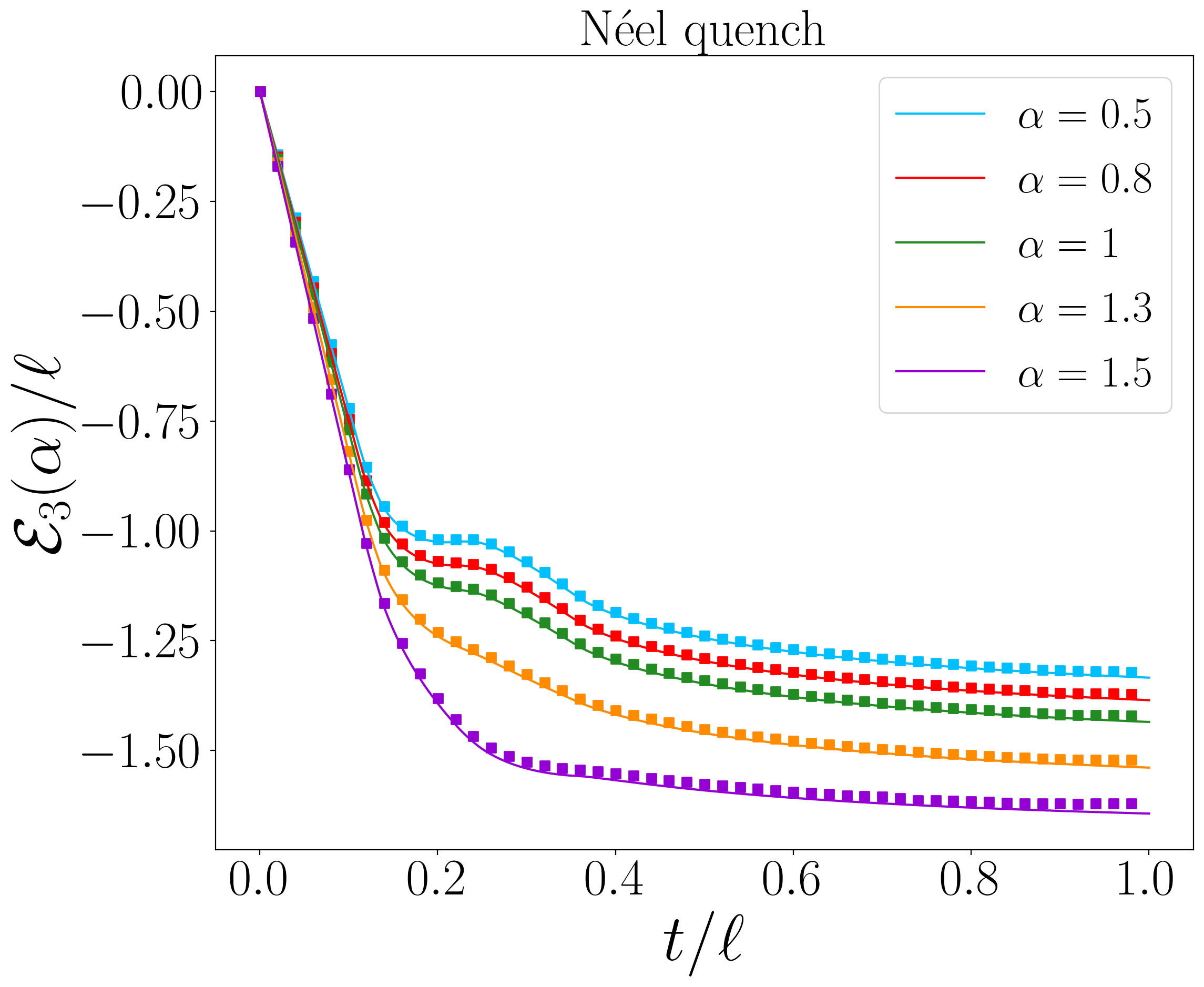
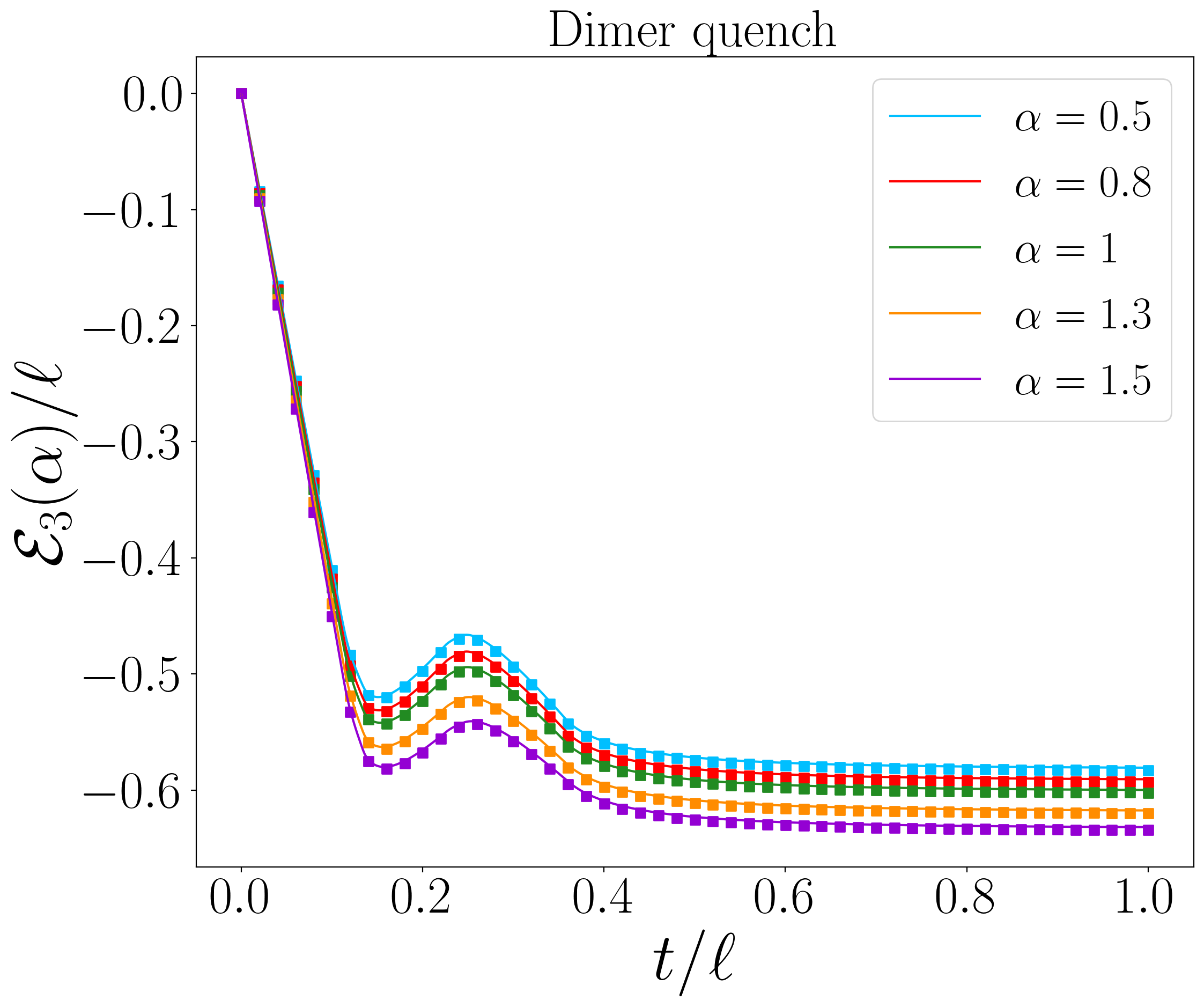
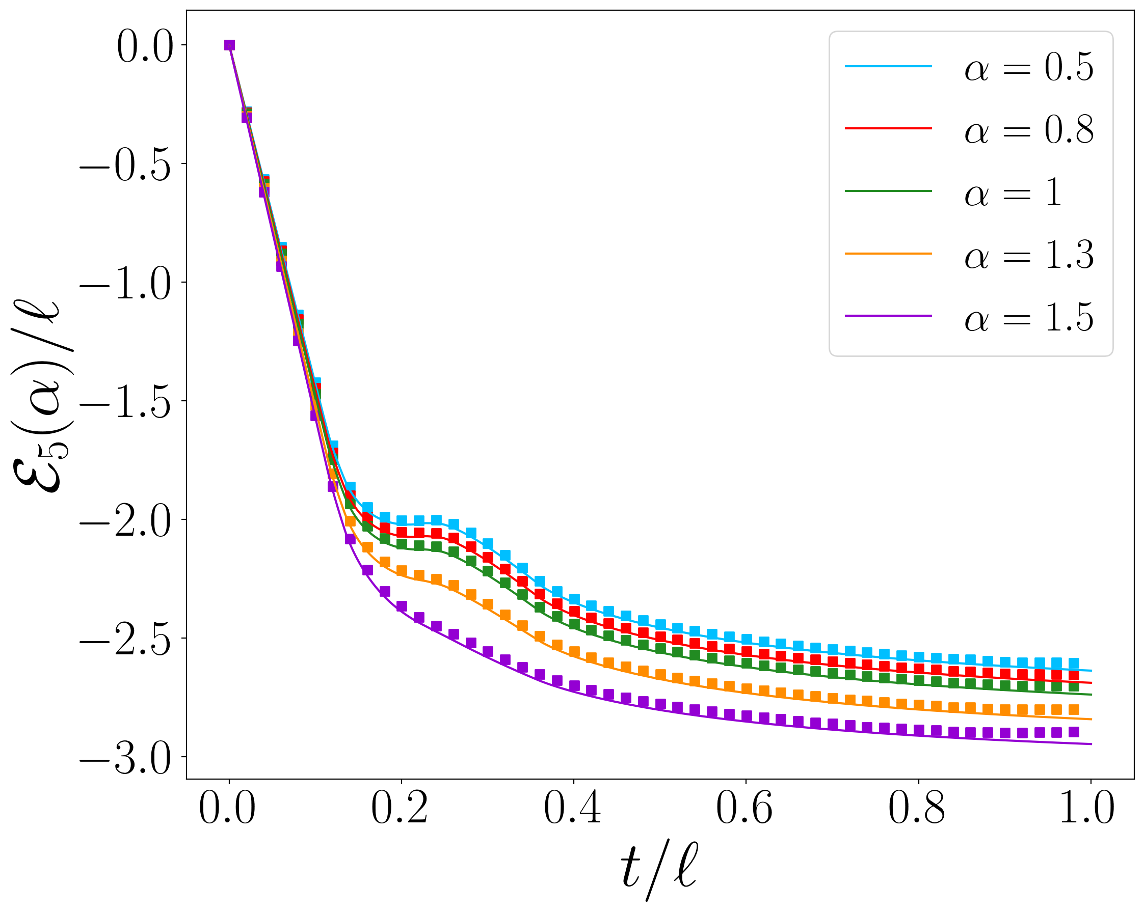
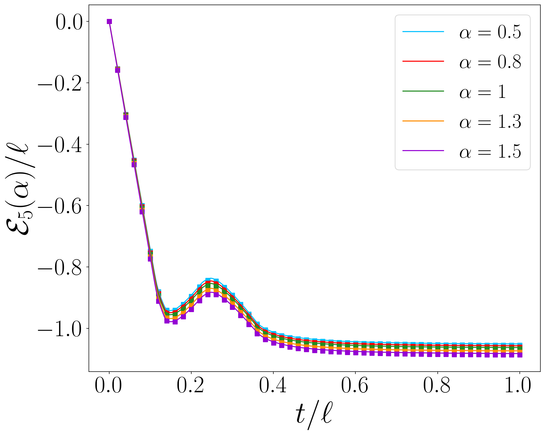
Figure 5: Time evolution of $\mathcal{E}_{n_{o}}(\alpha)$ with $n_{o}=3,5$ after a quench from the Néel state (left) and the dimer state (right) in the tight-biding model (3.1) as a function of $t/\ell$ with $\ell_{1}=230$, $\ell_{2}=270$ and $d=220$. The conjecture of Eq. (4.7) (solid lines) perfectly matches the numerical data (symbols).

5 Charge-imbalance-resolved negativity

In this section, we investigate the charge-imbalance-resolved negativity after the two quenches under consideration. Looking at (2.19), we need to compute the Fourier transform of the charged logarithmic negativity $\mathcal{E}(\alpha)$ and the charged probability $N_{1}(\alpha)$ to obtain $\mathcal{Z}_{R_{1}}(q)$ and $p(q)$, given in Eqs. (2.18) and (2.16), respectively. We also recover known results for the quench dynamics of the total logarithmic negativity from the charge-imbalance-resolved ones.

5.1 Fourier transforms

To compute the Fourier transforms, we approximate the charged negativity and probability at quadratic order in $\alpha$. We introduce the integrals

$$\begin{split}\mathcal{J}_{A_{1},A_{2}}^{(1)}&=\int\frac{\mathrm{d}k}{2\pi}(1-x_{k}^{2})(\min(\ell_{1},2v_{k}t)+\min(\ell_{2},2v_{k}t)),\\ \mathcal{J}_{m}^{(1)}&=\int\frac{\mathrm{d}k}{2\pi}(1-x_{k}^{2})(\max(d,2v_{k}t)+\max(d+\ell,2v_{k}t)-\max(d+\ell_{1},2v_{k}t)-\max(d+\ell_{2},2v_{k}t)),\\ \mathcal{J}_{m}^{(1/2)}&=\int\frac{\mathrm{d}k}{2\pi}\frac{2}{1+(1-x_{k}^{2})^{-1/2}}(\max(d,2v_{k}t)+\max(d+\ell,2v_{k}t)-\max(d+\ell_{1},2v_{k}t)-\max(d+\ell_{2},2v_{k}t)),\end{split}$$ (5.1)

and find

$$\begin{split}\mathcal{E}(\alpha)&=\mathcal{E}(0)-\frac{\alpha^{2}}{8}\big{(}\mathcal{J}_{A_{1},A_{2}}^{(1)}-\mathcal{J}_{m}^{(1)}+\mathcal{J}_{m}^{(1/2)}\big{)}+\mathcal{O}(\alpha^{4}),\\[14.22636pt] \mathcal{E}_{1}(\alpha)&=-\frac{\alpha^{2}}{8}\big{(}\mathcal{J}_{A_{1},A_{2}}^{(1)}+\mathcal{J}_{m}^{(1)}\big{)}+\mathcal{O}(\alpha^{4}),\end{split}$$ (5.2)

where

$$\mathcal{E}(0)=\int\frac{\mathrm{d}k}{2\pi}h_{1/2,0}(x_{k})(\max(d,2v_{k}t)+\max(d+\ell,2v_{k}t)-\max(d+\ell_{1},2v_{k}t)-\max(d+\ell_{2},2v_{k}t)).$$ (5.3)

From the definitions (2.4) and (2.15), this quantity is the total logarithmic negativity, $\mathcal{E}(0)\equiv\mathcal{E}$.

Next, we evaluate the Fourier transform of these quantities with respect to the charge-imbalance operator $\hat{Q}_{A}=Q_{1}+Q_{2}-\ell/2$ with charge $q=\Delta q+\langle\hat{Q}_{A}\rangle$. In both quenches, we have $\langle\hat{Q}_{A}\rangle=0$, and the integrals yield

$$\mathcal{Z}_{R_{1}}(q) =\mathrm{e}^{\mathcal{E}(0)}\int_{-\pi}^{\pi}\frac{d\alpha}{2\pi}\mathrm{e}^{-\mathrm{i}\Delta q\alpha}\mathrm{e}^{-\frac{\alpha^{2}}{8}(\mathcal{J}_{A_{1},A_{2}}^{(1)}-\mathcal{J}_{m}^{(1)}+\mathcal{J}_{m}^{(1/2)})}$$ (5.4)

$$=\mathrm{e}^{\mathcal{E}(0)}\mathrm{e}^{-\frac{2\Delta q^{2}}{\mathcal{J}_{A_{1},A_{2}}^{(1)}-\mathcal{J}_{m}^{(1)}+\mathcal{J}_{m}^{(1/2)}}}\sqrt{\frac{2}{\pi(\mathcal{J}_{A_{1},A_{2}}^{(1)}-\mathcal{J}_{m}^{(1)}+\mathcal{J}_{m}^{(1/2)})}},$$

$$p(q) =\int_{-\pi}^{\pi}\frac{d\alpha}{2\pi}\mathrm{e}^{-\mathrm{i}\Delta q\alpha}\mathrm{e}^{-\frac{\alpha^{2}}{8}(\mathcal{J}_{A_{1},A_{2}}^{(1)}+\mathcal{J}_{m}^{(1)})}$$ (5.5)

$$=\mathrm{e}^{-\frac{2\Delta q^{2}}{\mathcal{J}_{A_{1},A_{2}}^{(1)}+\mathcal{J}_{m}^{(1)}}}\sqrt{\frac{2}{\pi(\mathcal{J}_{A_{1},A_{2}}^{(1)}+\mathcal{J}_{m}^{(1)})}}.$$

We note that for the Néel quench there is a closed-form expression for $\mathcal{Z}_{R_{1}}(q)$ in terms of Gamma functions, similar to the charged entropies given in [34] for the same quench. We do not report this expression here, since it yields the same results as Eq. (5.4) in the limit $|\Delta q|\ll\ell$. Moreover, there is no closed-form expression for $p(q)$, and hence we de not have an exact result for the charge-imbalance-resolved logarithmic negativity $\hat{\mathcal{E}}(q)$.

5.2 Charge-imbalance-resolved logarithmic negativity

We insert Eqs. (5.4) and (5.5) in (2.19) and find

$$\hat{\mathcal{E}}(q)=\mathcal{E}(0)-2\Delta q^{2}\Big{(}\frac{1}{\mathcal{J}_{A_{1},A_{2}}^{(1)}-\mathcal{J}_{m}^{(1)}+\mathcal{J}_{m}^{(1/2)}}-\frac{1}{\mathcal{J}_{A_{1},A_{2}}^{(1)}+\mathcal{J}_{m}^{(1)}}\Big{)}+\frac{1}{2}\log\Big{(}\frac{\mathcal{J}_{A_{1},A_{2}}^{(1)}+\mathcal{J}_{m}^{(1)}}{\mathcal{J}_{A_{1},A_{2}}^{(1)}-\mathcal{J}_{m}^{(1)}+\mathcal{J}_{m}^{(1/2)}}\Big{)}.$$ (5.6)

We stress that this result holds in the limit $|\Delta q|\ll\ell$. We compare the prediction of Eq. (5.6) with ab initio numerical results in Fig. 6 and find a convincing match for small values of $|\Delta q|$. To understand the qualitative behaviour of the charge-imbalance-resolved negativity, let us discuss the $\mathcal{J}$-integrals in Eq. (5.1). We suppose without loss of generality that $\ell_{1}\leqslant\ell_{2}$. The integral $\mathcal{J}_{A_{1},A_{2}}^{(1)}$ has two distinct regimes. For $t\leqslant\ell_{1}/(2v_{\max})$, it grows linearly with $t$, whereas it saturates to a value proportional to $\ell$ in the limit $t\to\infty$. The integrals $\mathcal{J}_{m}^{(1)}$ and $\mathcal{J}_{m}^{(1/2)}$ both vanish for $t\leqslant d/(2v_{\max})$ and in the limit $t\to\infty$, and reach a value proportional to $\ell$ for intermediate times. Looking at (5.6), we thus conclude that there is an equipartition broken at order $\Delta q^{2}/\ell$ for intermediate times, whereas the equipartition is exact for $t\leqslant d/(2v_{max})$ and in the limit $t\to\infty$. These behaviours are well reproduced by our numerical analysis in Fig. 6, and are reminiscent of the quench dynamics of the symmetry-resolved mutual information discussed in [34]. This is not surprising, since it is known that the total logarithmic negativity and mutual information have a similar behaviour out of equilibrium [103, 104].

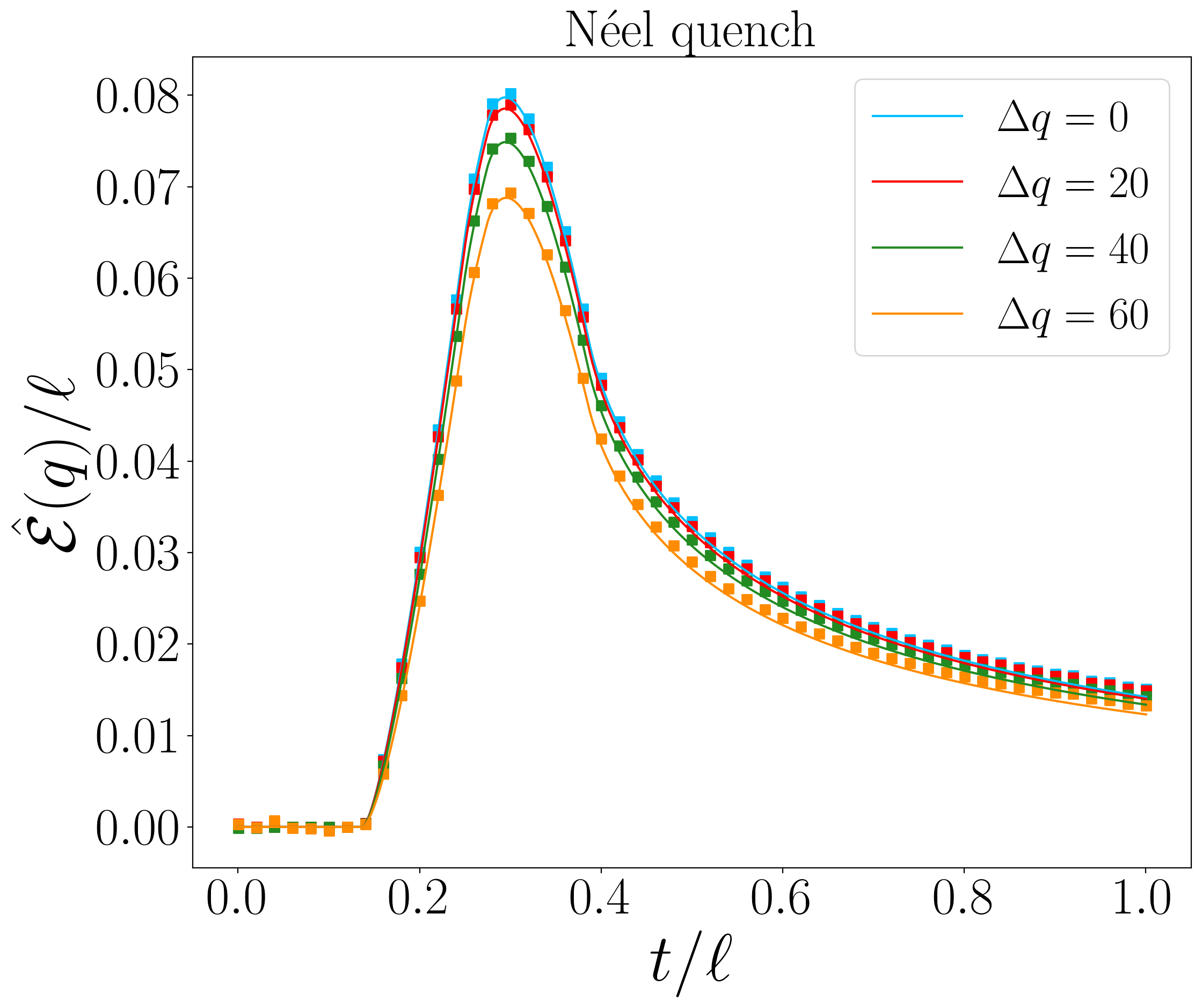
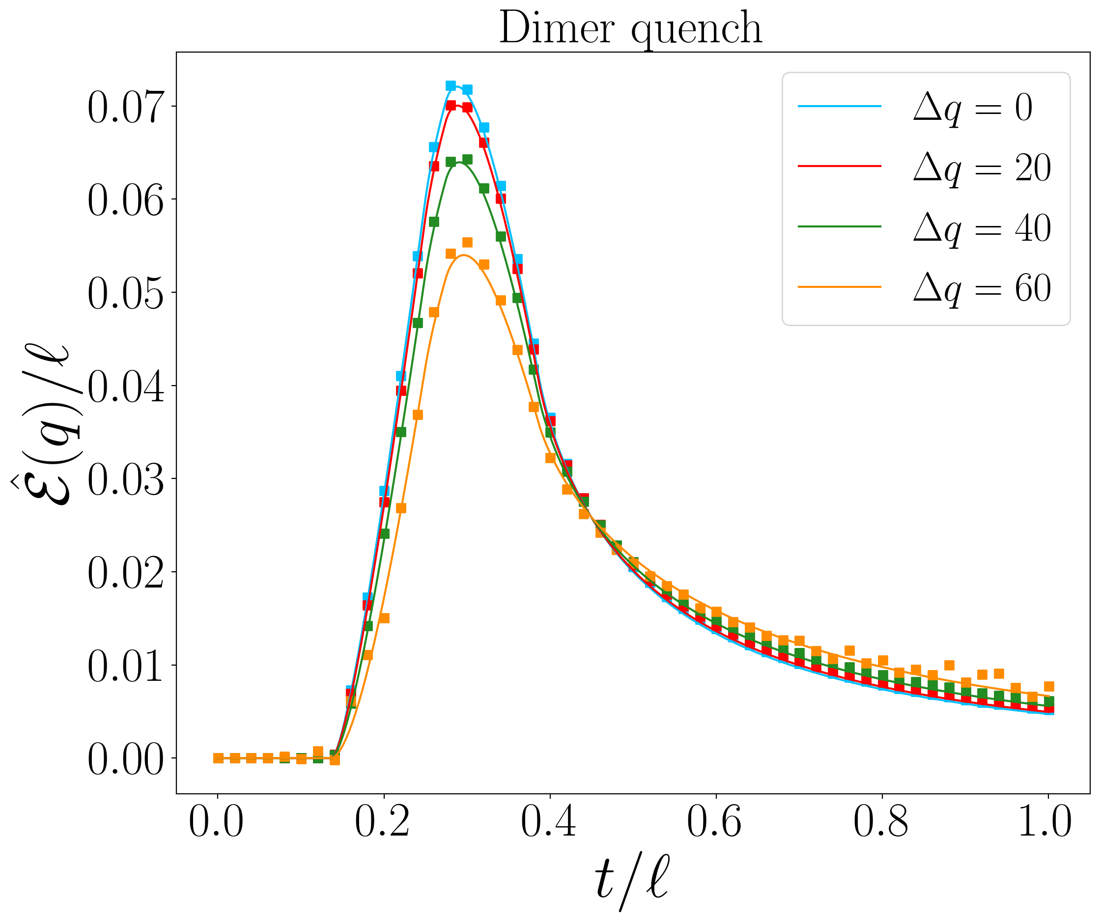
Figure 6: Time evolution of $\hat{\mathcal{E}}(q)$ after a quench from the Néel state (left) and the dimer state (right) in the tight-biding model (3.1) as a function of $t/\ell$ with $\ell_{1}=180$, $\ell_{2}=220$ and $d=220$. The approximation of Eq. (5.6) (solid lines) matches the numerical data (symbols) convincingly for small values of $|\Delta q|$ and start deviating from the data as $|\Delta q|$ increases considerably.

5.3 Total negativity

To check the consistency of our results, we wish to recover the total negativity from the charge-imbalance-resolved ones. We recast Eq. (2.11) as

$$\mathcal{N}=\sum_{q=-\ell/2}^{\ell/2}p(q)\frac{\mathrm{e}^{\hat{\mathcal{E}}(q)}-1}{2}.$$ (5.7)

For clarity, we consider the two sums in the right-hand side separately. With the quadratic approximations of Eqs. (5.5) and (5.6), we have

$$\begin{split}\sum_{q=-\ell/2}^{\ell/2}p(q)&=\sqrt{\frac{2}{\pi(\mathcal{J}_{A_{1},A_{2}}^{(1)}+\mathcal{J}_{m}^{(1)})}}\sum_{\Delta q=-\ell/2}^{\ell/2}\mathrm{e}^{-\frac{2\Delta q^{2}}{\mathcal{J}_{A_{1},A_{2}}^{(1)}+\mathcal{J}_{m}^{(1)}}},\\[8.5359pt] \sum_{q=-\ell/2}^{\ell/2}p(q)\mathrm{e}^{\hat{\mathcal{E}}(q)}&=\mathrm{e}^{\mathcal{E}(0)}\sqrt{\frac{2}{\pi(\mathcal{J}_{A_{1},A_{2}}^{(1)}-\mathcal{J}_{m}^{(1)}+\mathcal{J}_{m}^{(1/2)})}}\sum_{\Delta q=-\ell/2}^{\ell/2}\mathrm{e}^{-\frac{2\Delta q^{2}}{\mathcal{J}_{A_{1},A_{2}}^{(1)}-\mathcal{J}_{m}^{(1)}+\mathcal{J}_{m}^{(1/2)}}}.\end{split}$$ (5.8)

We note that the quadratic approximations are valid for $|\Delta q|\ll\ell$, and this condition is not met for the extreme values of $\Delta q$ in the sum. However, these values for the subsystem charge have a very low probability, and we nonetheless expect these approximations to give good results. Similar approximations provided excellent results for the total entanglement entropy, see [34]. Both terms in Eq. (5.8) have the form $\sqrt{\frac{2}{\pi\mathcal{J}}}\sum_{\Delta q=-\ell/2}^{\ell/2}\mathrm{e}^{-\frac{2\Delta q^{2}}{\mathcal{J}}}$ for some $\mathcal{J}>0$. In the large-$\ell$ limit, we approximate the sums as integrals over the real axis, and use the Gaussian integral

$$\sqrt{\frac{2}{\pi\mathcal{J}}}\int_{-\infty}^{\infty}\mathrm{d}\Delta q\ \mathrm{e}^{-\frac{2\Delta q^{2}}{\mathcal{J}}}=1.$$ (5.9)

This simplifies both terms in Eq. (5.8). With Eq. (5.7), we conclude

$$\mathcal{N}=\frac{\mathrm{e}^{\mathcal{E}(0)}-1}{2},$$ (5.10)

where $\mathcal{E}(0)$ is the total logarithmic negativity given in Eq. (5.3). We thus recover the known quench dynamics for the total logarithmic negativity from the charge-imbalance-resolved ones [103].

6 Quasiparticle picture for the charged Rényi logarithmic negativities

In this section, we discuss a physical picture, known as the quasiparticle picture [15, 18, 19], that allows one to predict the time evolution of entanglement measures after a global quantum quench from a low-entangled initial state in a one-dimensional quantum integrable model. In particular, we argue that our results for the charged Rényi logarithmic negativities can be understood in terms of the quasiparticle picture, and generalise recent results for the dynamics of Rényi logarithmic negativities [76].

6.1 Quasiparticle picture and entanglement dynamics for free fermions

In the global quench protocol, the system is prepared in an initial state $|\psi_{0}\rangle$ that has an extensive amount of energy compared to the groundstate of the Hamiltonian $H$ which governs the subsequent time evolution. Because of this surplus of energy, the initial state acts as a source of quasiparticle excitations, which are assumed to be produced in independent pairs with opposite momenta $k$ and $-k$. This assumption can be weakened in free models [105, 106, 107], but it is fundamental for interacting integrable systems, as argued in [108]. After the quench, each particle moves ballistically through the system, with velocity $v_{k}$. For spin chains with local interactions, the Lieb-Robinson bound [109] guarantees that there is a maximum value $v_{\max}$ for the possible velocities of the quasiparticles. The key element of this description is that the quasiparticles emitted from different points are incoherent, while those emitted from the same point are entangled. The entanglement between a subsystem $A$ and its complement $B$ is thus proportional to the number of entangled pairs of quasiparticles shared between $A$ and $B$. In the case where $A$ is a single interval of length $\ell$ embedded in an infinite line, the quasiparticle picture predicts that the entanglement entropy evolves as [15]

$$S_{1}(t)=2t\int_{2v_{k}t<\ell}\mathrm{d}k\ v_{k}s(k)+\ell\int_{2v_{k}t>\ell}\mathrm{d}k\ s(k)$$ (6.1)

in the scaling limit $\ell,t\to\infty$ with fixed ratio $t/\ell$. Here, the function $s(k)$ depends on the rate of production of the quasiparticles with momentum $\pm k$ and their contribution to the entanglement entropy. This situation is illustrated in Fig. 7. The two terms of Eq. (6.1) give two different regimes as the entropy evolves in time. For times $t\leqslant\ell/(2v_{\max})$, the domain of integration of the second integral vanishes, and the entropy grows linearly in time. For larger times, the entanglement entropy growth slows down, and for $t\gg\ell/(2v_{\max})$ the entanglement entropy saturates to a value that is extensive in the subsystem size.

Figure 7: Illustration of the quasiparticle picture for the entanglement spreading in a one-dimensional integrable system. The arrows indicate the propagation of the quasiparticles with the largest velocity $v_{\max}$.

To give predictive power to the quasiparticle result (6.1), one needs to compute the function $s(k)$, which depends strongly on the model and on the initial state. For free-fermion models, this function reads [18]

$$s(k)=\frac{1}{2\pi}(-n_{k}\log n_{k}-(1-n_{k})\log(1-n_{k}))$$ (6.2)

where $n_{k}$ is the probability of occupation of the mode $k$ in the stationary state. The result (6.1) also holds for the Rényi entropies $S_{n}$ with the replacement [110]

$$s(k)\to s_{n}(k)=\frac{1}{2\pi}\frac{1}{1-n}\log(n_{k}^{n}+(1-n_{k})^{n}).$$ (6.3)

In terms of the function $h_{n,\alpha}(x)$ defined in Eq. (4.1), we thus have

$$S_{n}(t)=\frac{1}{1-n}\int\frac{\mathrm{d}k}{2\pi}h_{n,0}(2n_{k}-1)\min(\ell,2v_{k}t)$$ (6.4)

where we use the function $\min(\ell,2v_{k}t)$ to recast the sum of two integrals in (6.1) in a simpler form. We mention that finding a generalisation of Eq. (6.1) for Rényi entropies with $n\neq 1$ was a long-standing open problem for interacting integrable models [110, 111, 112, 113, 114] which has been solved only very recently [115].

6.2 Quasiparticle dynamics for the charged Rényi logarithmic negativities

Figure 8: Illustration of the entanglement dynamics between disjoint intervals in the case where there is a single velocity for the quasiparticles. At a given time $t$, the number of quasiparticles shared between $A_{1}$ and $A_{2}$ is proportional to the width of the darker orange region. The typical behaviour of the logarithmic negativity is reported on the vertical plot on the left. It illustrates the delay before the linear increase, the plateau and the linear decrease discussed in the main text.

Let us consider the case in which the subsystem $A$ of length $\ell$ consists of two disjoint intervals $A_{1}$ and $A_{2}$ of respective lengths $\ell_{1}$ and $\ell_{2}$ that are separated by a distance $d$. Without loss of generality we consider $\ell_{1}\leqslant\ell_{2}$. In this case, the dynamics of the logarithmic negativity can be understood in terms of the quasiparticle picture. The entanglement between $A_{1}$ and $A_{2}$ is proportional to the number of pairs of entangled quasiparticles they share at a given time $t$. To ease the counting exercise, let us first assume that all the quasiparticles have the same velocity $v_{k}=v$. It follows that for short times $t\leqslant d/(2v)$, there are no entangled quasiparticles shared by the two intervals and the logarithmic negativity is zero. It then increases linearly for $d/(2v)\leqslant t\leqslant(d+\ell_{1})/(2v)$. There is a plateau for $(d+\ell_{1})/(2v)\leqslant t\leqslant(d+\ell_{2})/(2v)$, after which it decreases linearly in time up to $t=(d+\ell)/(2v)$. There are no longer any quasiparticles shared between the subsystems for larger times, so that the logarithmic negativity vanishes for $t\geqslant(d+\ell)/(2v)$. We illustrate this behaviour in Fig. 8. Accordingly, the resulting dynamics of the logarithmic negativity is proportional to $(\max(d,2vt)+\max(d+\ell,2vt)-\max(d+\ell_{1},2vt)-\max(d+\ell_{2},2vt))$[116, 95].

In the presence of different velocities $v_{k}$, the quasiparticle result is [18, 19]

$$\mathcal{E}=\int\frac{\mathrm{d}k}{2\pi}\ \epsilon(k)(\max(d,2v_{k}t)+\max(d+\ell,2v_{k}t)-\max(d+\ell_{1},2v_{k}t)-\max(d+\ell_{2},2v_{k}t)),$$ (6.5)

with $\epsilon(k)=h_{1/2,0}(2n_{k}-1)$ for free fermions. We note that this is exactly what we find in Eq. (5.3) for the total logarithmic negativity, with $n_{k}=1/2$ for the quench from the Néel state, and $n_{k}=(1+\cos k)/2$ for the dimer state.

The quasiparticle picture also describes the dynamics of the Rényi logarithmic negativities $\mathcal{E}_{n}$ defined in (2.5). The result is [76]

$$\mathcal{E}_{n}=\int\frac{\mathrm{d}k}{2\pi}\epsilon_{n}(k)(\min(\ell_{1},2v_{k}t)+\min(\ell_{2},2v_{k}t))\\ -\int\frac{\mathrm{d}k}{2\pi}(\epsilon_{n}(k)-\epsilon^{(2)}_{n}(k))(\max(d,2v_{k}t)+\max(d+\ell,2v_{k}t)-\max(d+\ell_{1},2v_{k}t)-\max(d+\ell_{2},2v_{k}t))$$ (6.6)

with

$$\epsilon^{(2)}_{n}(k)=\begin{cases}\frac{1}{2}\epsilon_{n}(k),&\mathrm{odd}\ n,\\[8.5359pt] \epsilon_{\frac{n}{2}}(k),&\mathrm{even}\ n.\end{cases}$$ (6.7)

For free systems, the kernels are

$$\epsilon_{n}(k)=h_{n,0}(2n_{k}-1)=\log(n_{k}^{n}+(1-n_{k})^{n}).$$ (6.8)

We note that the limit $n_{e}\to 1$ of Eq. (6.6) for even $n_{e}$ yields Eq. (6.5), as expected, because $h_{1,0}(x)=0$.

Our results of Eqs. (4.6) and (4.7) for the charged Rényi logarithmic negativities suggest the quasiparticle conjecture

$$\mathcal{E}_{n}(\alpha)=\mathrm{i}\alpha\langle\hat{Q}_{A}\rangle+\int\frac{\mathrm{d}k}{2\pi}\epsilon_{n,\alpha}(k)(\min(\ell_{1},2v_{k}t)+\min(\ell_{2},2v_{k}t))\\ -\int\frac{\mathrm{d}k}{2\pi}(\epsilon_{n,\alpha}(k)-\epsilon^{(2)}_{n,\alpha}(k))(\max(d,2v_{k}t)+\max(d+\ell,2v_{k}t)-\max(d+\ell_{1},2v_{k}t)-\max(d+\ell_{2},2v_{k}t))$$ (6.9)

with

$$\epsilon^{(2)}_{n,\alpha}(k)=\begin{cases}\frac{1}{2}\epsilon_{n,2\alpha}(k),&\mathrm{odd}\ n,\\[8.5359pt] \epsilon_{\frac{n}{2},\alpha}(k),&\mathrm{even}\ n.\end{cases}$$ (6.10)

Here, $\epsilon_{n,0}(k)\equiv\epsilon_{n}(k)$ from Eq. (6.6), and $\epsilon_{n,\alpha}(k)=\mathrm{Re}[h_{n,\alpha}(2n_{k}-1)]$ for free systems. Even though this conjecture is similar to Eq. (6.6) and the results of [76], the $\alpha$-dependence in Eq. (6.10) is non-trivial and could not have been directly guessed from the results for the total Rényi logarithmic negativities.

We expect that qualitatively similar results apply also to generic integral models. However, the known problems for the calculation of the Rényi entropies [110, 111, 112] still prevent from the determination of the exact kernels in the integral (6.9) that would replace $\epsilon_{n,\alpha}(k)$ and $\epsilon^{(2)}_{n,\alpha}(k)$. The first steps towards the solution of these issues were recently discussed in the literature [74, 115].

7 Conclusion

In this paper, we investigated the dynamics of the charge-imbalance-resolved negativity after a quench in a free-fermion chain. We first considered the corresponding charged moments $N_{n}(\alpha)$, and expressed these quantities in terms of the two-point correlation matrix. Second, we used these formulas to give analytical results and conjectures for the charged Rényi logarithmic negativities $\mathcal{E}_{n}(\alpha)$. We tested those results against ab initio numerical computations for two distinct quenches, and found a systematic very good agreement. Third, we studied the Fourier transforms of the charged moments approximated at quadratic order in $\alpha$ to investigate the charge-imbalance-resolved negativity. Our results show a perfect equipartition for early and large times that is broken at order $\Delta q^{2}/\ell$ for intermediate ones. These results hold in the limit $|\Delta q|\ll\ell$, and match numerical results with a satisfactory precision. Finally, we argued that our results for the charged Rényi logarithmic negativities can be understood in the framework of the quasiparticle picture for the entanglement dynamics, and we provided a conjecture for $\mathcal{E}_{n}(\alpha)$ that we expect to hold for a large variety of integrable models with a proper adaptation.

There are several avenues that would be worth investigating in the future. First, it would be natural to test our quasiparticle conjecture for the charged Rényi logarithmic negativities $\mathcal{E}_{n}(\alpha)$ (as well as the conjectures for the charged entropies and mutual information, see [33, 34]) in the context of interacting integrable models. A second idea is to investigate symmetry-resolved entanglement measures after an inhomogeneous quench, similarly to the total entanglement entropy in Refs. [117, 118, 119, 120, 121, 122]. Finally, it would be necessary to understand whether one could compute symmetry-resolved entanglement measure for non-integrable models with some of the methods developed in e.g. Refs. [123, 124, 125, 128, 129, 130, 131, 132, 126, 127, 133, 134].

References

- [1] A. Polkovnikov, K. Sengupta, A. Silva, and M. Vengalattore, Colloquium: Nonequilibrium dynamics of closed interacting quantum systems, Rev. Mod. Phys. 83, 863 (2011).
- [2] C. Gogolin and J. Eisert, Equilibration, thermalisation, and the emergence of statistical mechanics in closed quantum systems, Rep. Prog. Phys. 79, 056001 (2016).
- [3] L. D’Alessio, Y. Kafri, A. Polkovnikov, and M. Rigol, From Quantum Chaos and Eigenstate Thermalization to Statistical Mechanics and Thermodynamics, Adv. Phys. 65, 239 (2016).
- [4] P. Calabrese, F. H. L. Essler, and G. Mussardo, Quantum Integrability in Out of Equilibrium Systems, J. Stat. Mech. 064001 (2016).
- [5] F. H. L. Essler and M. Fagotti, Quench dynamics and relaxation in isolated integrable quantum spin chains, J. Stat. Mech. 064002 (2016).
- [6] P. Calabrese, Entanglement and thermodynamics in non-equilibrium isolated quantum systems, Physica A 504, 31 (2018).
- [7] J. M. Deutsch, H. Li, and A. Sharma, Microscopic origin of thermodynamic entropy in isolated systems, Phys. Rev. E 87, 042135 (2013).
- [8] L. F. Santos, A. Polkovnikov, and M. Rigol, Entropy of Isolated Quantum Systems after a Quench, Phys. Rev. Lett. 107, 040601 (2011).
- [9] M. Collura, M. Kormos, and P. Calabrese, Stationary entropies following an interaction quench in Bose gas, J. Stat. Mech. P01009 (2014).
- [10] N. Schuch, M. M. Wolf, F. Verstraete, and J. I. Cirac, Entropy Scaling and Simulability by Matrix Product States, Phys. Rev. Lett. 100, 030504 (2008).
- [11] N. Schuch, M. M. Wolf, K. G. H. Vollbrecht, and J. I. Cirac, On entropy growth and the hardness of simulating time evolution, New J. Phys. 10, 033032 (2008).
- [12] A. Perales and G. Vidal, Entanglement growth and simulation efficiency in one-dimensional quantum lattice systems, Phys. Rev. A 78, 042337 (2008).
- [13] P. Hauke, F. M. Cucchietti, L. Tagliacozzo, I. Deutsch, and M. Lewenstein, Can one trust quantum simulators? Prog. Phys. 75, 082401 (2012).
- [14] J. Dubail, Entanglement scaling of operators: a conformal field theory approach, with a glimpse of simulability of long-time dynamics in 1+1d, J. Phys. A 50, 234001 (2017).
- [15] P. Calabrese and J. Cardy, Evolution of Entanglement Entropy in One-Dimensional Systems, J. Stat. Mech. P04010 (2005).
- [16] P. Calabrese and J. Cardy, Time-dependence of correlation functions following a quantum quench, Phys. Rev. Lett. 96, 136801 (2006).
- [17] P. Calabrese and J. Cardy, Quantum Quenches in Extended Systems, J. Stat. Mech. P06008 (2007).
- [18] V. Alba and P. Calabrese, Entanglement and thermodynamics after a quantum quench in integrable systems, PNAS 114, 7947 (2017).
- [19] V. Alba and P. Calabrese, Entanglement dynamics after quantum quenches in generic integrable systems, SciPost Phys. 4, 017 (2018).
- [20] P. Calabrese, Entanglement spreading in non-equilibrium integrable systems, Lectures for Les Houches Summer School on “Integrability in Atomic and Condensed Matter Physics", SciPost Phys. Lect. Notes 20 (2020).
- [21] A. M. Kaufman, M. E. Tai, A. Lukin, M. Rispoli, R. Schittko, P. M. Preiss, and M. Greiner, Quantum thermalisation through entanglement in an isolated many-body system, Science 353, 794 (2016).
- [22] A. Lukin, M. Rispoli, R. Schittko, M. E. Tai, A. M. Kaufman, S. Choi, V. Khemani, J. Leonard, and M. Greiner, Probing entanglement in a many-body localized system, Science 364, 6437 (2019).
- [23] T. Brydges, A. Elben, P. Jurcevic, B. Vermersch, C. Maier, B. P. Lanyon, P. Zoller, R. Blatt, and C. F. Roos, Probing entanglement entropy via randomized measurements, Science 364, 260 (2019).
- [24] A. Elben, R. Kueng, H.-Y. Huang, R. van Bijnen, C. Kokail, M. Dalmonte, P. Calabrese, B. Kraus, J. Preskill, P. Zoller, and B. Vermersch, Mixed-state entanglement from local randomized measurements, Phys. Rev. Lett. 125, 200501 (2020).
- [25] M. M. Wolf, F. Verstraete, M.B. Hastings, and I. J. Cirac, Area Laws in Quantum Systems: Mutual Information and Correlations, Phys. Rev. Lett. 100, 070502 (2008).
- [26] G. Vidal and R. F. Werner Computable measure of entanglement, Phys. Rev. A 65, 032314 (2002).
- [27] A. Peres, Separability Criterion for Density Matrices Phys. Rev. Lett. 77, 1413 (1996).
- [28] R. Simon, Peres-Horodecki Separability Criterion for Continuous Variable Systems, Phys. Rev. Lett. 84, 2726 (2000).
-
[29]
M. B. Plenio, Logarithmic Negativity: A Full Entanglement Monotone That is not Convex,
Phys. Rev. Lett. 95, 090503 (2005);
J. Eisert, Entanglement in quantum information theory, arXiv:quant-ph/0610253. - [30] A. Neven, J. Carrasco, V. Vitale, C. Kokail, A. Elben, M. Dalmonte, P. Calabrese, P. Zoller, B. Vermersch, R. Kueng, and B. Kraus, Symmetry-resolved entanglement detection using partial transpose moments, npj Quantum Inf 7, 152 (2021).
- [31] J. Gray, L. Banchi, A. Bayat, and S. Bose, Machine Learning Assisted Many-Body Entanglement Measurement, Phys. Rev. Lett. 121, 150503 (2018).
- [32] E. Cornfeld, E. Sela, and M. Goldstein, Measuring fermionic entanglement: Entropy, negativity, and spin structure, Phys. Rev. A 99, 062309 (2019).
- [33] G. Parez, R. Bonsignori and P. Calabrese, Quasiparticle dynamics of symmetry-resolved entanglement after a quench: Examples of conformal field theories and free fermions Phys. Rev. B 103, L041104 (2021).
- [34] G. Parez, R. Bonsignori and P. Calabrese, Exact quench dynamics of symmetry resolved entanglement in a free fermion chain J. Stat. Mech. 093102 (2021).
- [35] N. Laflorencie and S. Rachel, Spin-resolved entanglement spectroscopy of critical spin chains and Luttinger liquids, J. Stat. Mech. P11013 (2014).
- [36] M. Goldstein and E. Sela, Symmetry Resolved Entanglement in Many-Body Systems, Phys. Rev. Lett. 120, 200602 (2018).
- [37] J. C. Xavier, F. C. Alcaraz, and G. Sierra, Equipartition of the entanglement entropy, Phys. Rev. B 98, 041106 (2018).
- [38] E. Cornfeld, M. Goldstein, and E. Sela, Imbalance Entanglement: Symmetry Decomposition of Negativity, Phys. Rev. A 98, 032302 (2018).
- [39] R. Bonsignori, P. Ruggiero, and P. Calabrese, Symmetry resolved entanglement in free fermionic systems, J. Phys. A: Math. Theor. 52, 475302 (2019).
- [40] N. Feldman and M. Goldstein, Dynamics of Charge-Resolved Entanglement after a Local Quench, Phys. Rev. B 100, 235146 (2019).
- [41] E. Cornfeld, L. A. Landau, K. Shtengel, and E. Sela, Entanglement spectroscopy of non-Abelian anyons: Reading off quantum dimensions of individual anyons, Phys. Rev. B 99, 115429 (2019).
- [42] R. Bonsignori and P. Calabrese, Boundary effects on symmetry resolved entanglement, J. Phys. A: Math. Theor. 54, 015005 (2020).
- [43] S. Fraenkel and M. Goldstein, Symmetry resolved entanglement: Exact results in 1d and beyond, J. Stat. Mech. 033106 (2020).
- [44] L. Capizzi, P. Ruggiero, and P. Calabrese, Symmetry resolved entanglement entropy of excited states in a CFT, J. Stat. Mech. 073101 (2020).
- [45] S. Murciano, G. Di Giulio, and P. Calabrese, Symmetry resolved entanglement in gapped integrable systems: a corner transfer matrix approach, SciPost Phys. 8, 046 (2020).
- [46] S. Murciano, G. Di Giulio, and P. Calabrese, Entanglement and symmetry resolution in two dimensional free quantum field theories, JHEP 08 (2020) 073.
- [47] P. Calabrese, M. Collura, G. Di Giulio, and S. Murciano, Full counting statistics in the gapped XXZ spin chain, EPL 129, 60007 (2020).
- [48] M. T. Tan and S. Ryu, Particle number fluctuations, Rényi and symmetry-resolved entanglement entropy in two-dimensional Fermi gas from multi-dimensional bosonisation, Phys. Rev. B 101, 235169 (2020).
- [49] S. Murciano, P. Ruggiero, and P. Calabrese, Symmetry resolved entanglement in two-dimensional systems via dimensional reduction, J. Stat. Mech. 083102 (2020).
- [50] X. Turkeshi, P. Ruggiero, V. Alba, and P. Calabrese, Entanglement equipartition in critical random spin chains, Phys. Rev. B 102, 014455 (2020).
- [51] K. Monkman and J. Sirker, Operational Entanglement of Symmetry-Protected Topological Edge States, Phys. Rev. Res. 2, 043191 (2020).
- [52] D. X. Horváth and P. Calabrese, Symmetry resolved entanglement in integrable field theories via form factor bootstrap, JHEP 11 (2020) 131.
- [53] D. Azses and E. Sela, Symmetry-resolved entanglement in symmetry-protected topological phases, Phys. Rev. B 102, 235157 (2020).
- [54] S. Murciano, R. Bonsignori, P. Calabrese, Symmetry decomposition of negativity of massless free fermions, SciPost Phys. 10, 111 (2021).
- [55] D. X. Horvath, L. Capizzi, and P. Calabrese, U(1) symmetry resolved entanglement in free 1+1 dimensional field theories via form factor bootstrap, JHEP 05 (2021) 197.
- [56] V. Vitale, A. Elben, R. Kueng, A. Neven, J. Carrasco, B. Kraus, P. Zoller, P. Calabrese, B. Vermersch, and M. Dalmonte, Symmetry-resolved dynamical purification in synthetic quantum matter, arXiv:2101.07814.
- [57] S. Fraenkel and M. Goldstein, Entanglement Measures in a Nonequilibrium Steady State: Exact Results in One Dimension, SciPost Phys. 11, 085 (2021).
- [58] B. Estienne, Y. Ikhlef and A. Morin-Duchesne, Finite-size corrections in critical symmetry-resolved entanglement, SciPost Phys. 10, 54 (2021).
- [59] H.-H. Chen, Symmetry decomposition of relative entropies in conformal field theory, JHEP 07 (2021) 084.
- [60] L. Capizzi and P. Calabrese, Symmetry resolved relative entropies and distances in conformal field theory, JHEP 10 (2021) 195.
- [61] D. X. Horvath, P. Calabrese, and O. A. Castro-Alvaredo, Branch Point Twist Field Form Factors in the sine-Gordon Model II: Composite Twist Fields and Symmetry Resolved Entanglement, arXiv:2105.13982.
- [62] L. Capizzi, D. X. Horvath, P. Calabrese, and O. A. Castro-Alvaredo, Entanglement of the 3-State Potts Model via Form Factor Bootstrap: Total and Symmetry Resolved Entropies, arXiv:2108.10935.
- [63] P. Calabrese, J. Dubail and S. Murciano, Symmetry-resolved entanglement entropy in Wess-Zumino-Witten models, JHEP 10 (2021) 67.
- [64] S. Zhao, C. Northe and R. Meyer, Symmetry-resolved entanglement in AdS3/CFT2 coupled to U(1) Chern-Simons theory, JHEP 7 (2021) 30.
- [65] K. Weisenberger, S. Zhao, C. Northe and R. Meyer, Symmetry-resolved entanglement for excited states and two entangling intervals in AdS3/CFT2, JHEP 12 (2021) 104.
- [66] Z. Ma and E. Sela, Symmetric separability criterion for number conserving mixed states, arXiv:2110.09388.
- [67] H.-H. Chen, Charged Rényi negativity of massless free bosons, arXiv:2111.11028.
- [68] B. Oblak, N. Regnault and B. Estienne, Equipartition of Entanglement in Quantum Hall States, arXiv:2112.13854.
- [69] N. Feldman, A. Kshetrimayum, J. Eisert and M. Goldstein, Entanglement estimation in tensor network states via sampling, arXiv:2202.04089.
- [70] F. Ares, S. Murciano and P. Calabrese, Symmetry-resolved entanglement in a long-range free-fermion chain, arXiv:2202.05874.
- [71] N. G. Jones, Symmetry-resolved entanglement entropy in critical free-fermion chains, arXiv:2202.11728.
- [72] M. Ghasemi, Universal Thermal Corrections to Symmetry-Resolved Entanglement Entropy and Full Counting Statistics, arXiv:2203.06708.
- [73] L. Capizzi, O. A. Castro-Alvaredo, C. De Fazio, M. Mazzoni and L. Santamaría-Sanz, Symmetry Resolved Entanglement of Excited States in Quantum Field Theory I: Free Theories, Twist Fields and Qubits, arXiv:2203.12556.
- [74] L. Piroli, E. Vernier, M. Collura and P. Calabrese, Thermodynamic symmetry resolved entanglement entropies in integrable systems, arXiv:2203.09158.
- [75] S. Baiguera, L. Bianchi, S. Chapman and D. A. Galante, Shape Deformations of Charged Rényi Entropies from Holography, arXiv:2203.15028.
- [76] S. Murciano and V. Alba and P. Calabrese, Quench dynamics of Rényi negativities and the quasiparticle picture, arXiv:2110.14589.
- [77] V. Eisler and Z. Zimborás, On the partial transpose of fermionic Gaussian states, New J. Phys. 17, 053048 (2015).
- [78] A. Coser, E. Tonni, and P. Calabrese, Partial transpose of two disjoint blocks in XY spin chains, J. Stat. Mech. P08005 (2015).
- [79] A. Coser, E. Tonni, and P. Calabrese, Towards entanglement negativity of two disjoint intervals for a one dimensional free fermion, J. Stat. Mech. 033116 (2016).
- [80] J. Eisert, V. Eisler and Z. Zimborás, Entanglement negativity bounds for fermionic Gaussian states, Phys. Rev. B 97, 165123 (2018).
- [81] H. Shapourian, K. Shiozaki, and S. Ryu, Partial time-reversal transformation and entanglement negativity in fermionic systems, Phys. Rev. B 95, 165101 (2017).
- [82] H. Shapourian, K. Shiozaki, and S. Ryu, Many-Body Topological Invariants for Fermionic Symmetry-Protected Topological Phases, Phys. Rev. Lett. 118, 216402 (2017).
- [83] K. Shiozaki, H. Shapourian, K. Gomi, and S. Ryu, Many-body topological invariants for fermionic short-range entangled topological phases protected by antiunitary symmetries, Phys. Rev. B 98, 035151 (2018).
- [84] H. Shapourian and S. Ryu, Entanglement negativity of fermions: monotonicity, separability criterion, and classification of few-mode states, Phys. Rev. A 99, 022310 (2019).
- [85] H. Shapourian and S. Ryu, Finite-temperature entanglement negativity of free fermions, J. Stat. Mech. 043106 (2019).
- [86] H. Shapourian, P. Ruggiero, S. Ryu, and P. Calabrese, Twisted and untwisted negativity spectrum of free fermions, SciPost Phys. 7, 037 (2019).
- [87] J. Kudler-Flam, H. Shapourian, and S. Ryu, The negativity contour: a quasi-local measure of entanglement for mixed states, SciPost Phys. 8, 063 (2020).
- [88] S. Murciano, V. Vitale, M. Dalmonte, and P. Calabrese, The Negativity Hamiltonian: An operator characterization of mixed-state entanglement, arXiv:2201.03989.
- [89] H. Shapourian, R. S. K. Mong, and S. Ryu, Anyonic Partial Transpose I: Quantum Information Aspects, arXiv:2012.02222.
- [90] P. Calabrese, J. Cardy, and E. Tonni, Entanglement Negativity in Quantum Field Theory, Phys. Rev. Lett. 109, 130502 (2012).
- [91] P. Calabrese, J. Cardy, and E. Tonni, Entanglement negativity in extended systems: a field theoretical approach, J. Stat. Mech. P02008 (2013).
- [92] P. Caputa, G. Mandal, and R. Sinha, Dynamical entanglement entropy with angular momentum and U(1) charge, JHEP 11 (2013) 052.
- [93] A. Belin, L.-Y. Hung, A. Maloney, S. Matsuura, R. C. Myers and T. Sierens, Holographic Charged Rényi Entropies, JHEP 12 (2013) 59.
- [94] P. Caputa, M. Nozaki, and T. Numasawa, Charged entanglement entropy of local operators, Phys. Rev. D 93, 105032 (2016).
- [95] V. Alba and P. Calabrese, Quantum information scrambling after a quantum quench, Phys. Rev. B 100, 115150 (2019).
- [96] M. Fagotti, On conservation laws, relaxation and pre-relaxation after a quantum quench, J. Stat. Mech. P03016 (2014).
- [97] M. C. Chung and I. Peschel, Density-matrix spectra of solvable fermionic systems, Phys. Rev. B 64, 064412 (2001).
- [98] I. Peschel, Calculation of reduced density matrices from correlation functions, J. Phys. A 36, L205 (2003).
- [99] I. Peschel and V. Eisler, Reduced density matrices and entanglement entropy in free lattice models, J. Phys. A 42, 504003 (2009).
- [100] S. Groha, F. Essler, and P. Calabrese, Full counting statistics in the transverse field Ising chain, SciPost Phys. 4, 043 (2018).
- [101] M. Fagotti and P. Calabrese, Evolution of entanglement entropy following a quantum quench: Analytic results for the XY chain in a transverse magnetic field, Phys. Rev. A 78, 010306(R).
- [102] G. Parez and R. Bonsignori, Analytical results for the entanglement dynamics of disjoint blocks in the XY spin chain, arXiv:2210.03637.
- [103] V. Alba and P. Calabrese, Quantum information dynamics in multipartite integrable systems, EPL 126, 60001 (2019).
- [104] B. Bertini, K. Klobas and T.-C. Lu, Entanglement Negativity and Mutual Information after a Quantum Quench: Exact Link from Space-Time Duality, arXiv:2203.17254.
- [105] B. Bertini, E. Tartaglia, and P. Calabrese, Entanglement and diagonal entropies after a quench with no pair structure, J. Stat. Mech. 063104 (2018).
- [106] A. Bastianello and P. Calabrese, Spreading of entanglement and correlations after a quench with intertwined quasiparticles, SciPost Phys. 5, 033 (2018).
- [107] A. Bastianello and M. Collura, Entanglement spreading and quasiparticle picture beyond the pair structure, SciPost Phys. 8, 045 (2020).
- [108] L. Piroli, B. Pozsgay, and E. Vernier, What is an integrable quench?, Nucl. Phys. B 925, 362 (2017).
- [109] E.H. Lieb, D. W. Robinson, The finite group velocity of quantum spin systems, Commun. Math. Phys. 28, 251 (1972).
- [110] V. Alba and P. Calabrese, Quench action and Rényi entropies in integrable systems, Phys. Rev. B 96, 115421 (2017).
- [111] V. Alba and P. Calabrese, Rényi entropies after releasing the Néel state in the XXZ spin-chain, J. Stat. Mech. 113105 (2017).
- [112] M. Mestyán, V. Alba, and P. Calabrese, Rényi entropies of generic thermodynamic macrostates in integrable systems, J. Stat. Mech. 083104 (2018).
- [113] O. A. Castro-Alvaredo, M. Lencses, I. M. Szecsenyi and J. Viti, Entanglement dynamics after a quench in Ising field theory: a branch point twist field approach, JHEP 12 (2019) 079.
- [114] K. Klobas and B. Bertini, Entanglement dynamics in Rule 54: exact results and quasiparticle picture, SciPost Phys. 11, 107 (2021)
- [115] B. Bertini, K. Klobas, V. Alba, G. Lagnese and P. Calabrese, Growth of Rényi Entropies in Interacting Integrable Models and the Breakdown of the Quasiparticle Picture, arXiv:2203.17264.
- [116] A. Coser, E. Tonni, and P. Calabrese, Entanglement negativity after a global quantum quench, J. Stat. Mech. P12017 (2014).
- [117] V. Alba, Entanglement and quantum transport in integrable systems, Phys. Rev. B 97, 245135 (2018).
- [118] B. Bertini, M. Fagotti, L. Piroli, and P. Calabrese, Entanglement evolution and generalised hydrodynamics: noninteracting systems, J. Phys. A 51, 39LT01 (2018).
- [119] V. Alba, B. Bertini, and M. Fagotti, Entanglement evolution and generalised hydrodynamics: interacting integrable systems, SciPost Phys. 7, 005 (2019).
- [120] V. Alba, Towards a generalized hydrodynamics description of Rényi entropies in integrable systems, Phys. Rev. B 99, 045150 (2019).
- [121] J. Dubail, J.-M. Stéphan, J. Viti, and P. Calabrese, Conformal field theory for inhomogeneous one-dimensional quantum systems: the example of non-interacting Fermi gases, SciPost Phys. 2, 002 (2017).
- [122] P. Ruggiero, P. Calabrese, B. Doyon, and J. Dubail, Quantum Generalized Hydrodynamics, Phys. Rev. Lett. 124, 140603 (2020).
- [123] A. Nahum, J. Ruhman, S. Vijay, and J. Haah, Quantum Entanglement Growth under Random Unitary Dynamics, Phys. Rev. X 7, 031016 (2017).
- [124] A. Nahum, S. Vijay, and J. Haah, Operator Spreading in Random Unitary Circuits, Phys. Rev. X 8, 021014 (2018).
- [125] T. Zhou and A. Nahum, The entanglement membrane in chaotic many-body systems, Phys. Rev. X 10, 031066 (2020).
- [126] A. Chan, A. De Luca, and J. T. Chalker, Solution of a minimal model for many-body quantum chaos, Phys. Rev. X 8, 041019 (2018).
- [127] A. J. Friedman, A. Chan, A. De Luca, and J. T. Chalker, Spectral statistics and many-body quantum chaos with conserved charge, Phys. Rev. Lett. 123, 210603 (2019).
- [128] B. Bertini, P. Kos, and T. Prosen, Entanglement Spreading in a Minimal Model of Maximal Many-Body Quantum Chaos, Phys. Rev. X 9, 021033 (2019).
- [129] S. Gopalakrishnan and A. Lamacraft, Unitary circuits of finite depth and infinite width from quantum channels, Phys. Rev. B 100, 064309 (2019).
- [130] B. Bertini and P. Calabrese, Prethermalisation and Thermalisation in the Entanglement Dynamics, Phys. Rev. B 102, 094303 (2020).
- [131] L. Piroli, B. Bertini, J. I. Cirac, and T. Prosen, Exact dynamics in dual-unitary quantum circuits, Phys. Rev. B 101, 094304 (2020).
- [132] R. Modak, V. Alba, and P. Calabrese, Entanglement revivals as a probe of scrambling in finite quantum systems, J. Stat. Mech. 083110 (2020).
- [133] T. Rakovszky, F. Pollmann, and C. W. von Keyserlingk, Sub-ballistic Growth of Rényi Entropies due to Diffusion, Phys. Rev. Lett. 122, 250602 (2019).
- [134] T. Chanda, J. Zakrzewski, M. Lewenstein and L. Tagliacozzo, Confinement and Lack of Thermalization after Quenches in the Bosonic Schwinger Model, Phys. Rev. Lett. 124, 180602 (2020).