Characterizing and Overcoming the Greedy Nature of Learning in Multi-modal Deep Neural Networks

Abstract

We hypothesize that due to the greedy nature of learning in multi-modal deep neural networks, these models tend to rely on just one modality while under-fitting the other modalities. Such behavior is counter-intuitive and hurts the models’ generalization, as we observe empirically. To estimate the model’s dependence on each modality, we compute the gain on the accuracy when the model has access to it in addition to another modality. We refer to this gain as the conditional utilization rate. In the experiments, we consistently observe an imbalance in conditional utilization rates between modalities, across multiple tasks and architectures. Since conditional utilization rate cannot be computed efficiently during training, we introduce a proxy for it based on the pace at which the model learns from each modality, which we refer to as the conditional learning speed. We propose an algorithm to balance the conditional learning speeds between modalities during training and demonstrate that it indeed addresses the issue of greedy learning. The proposed algorithm improves the model’s generalization on three datasets: Colored MNIST, ModelNet40, and NVIDIA Dynamic Hand Gesture.

1 Introduction

In real-world problems, each instance frequently has multiple modalities associated with it. For example, we detect cancer in both X-ray and ultrasound images. We seek clues from images to answer questions given in text. We are naturally interested in training deep neural networks (DNNs) end-to-end to learn from all available input modalities. We refer to such a training regime as a multi-modal learning process and DNNs resulting from it as multi-modal DNNs.

Several recent studies have reported unsatisfactory performance of multi-modal DNNs in various tasks (Wang et al., 2020a; Wu et al., 2020; Gat et al., 2020; Cadene et al., 2019; Agrawal et al., 2016; Hessel & Lee, 2020; Han et al., 2021b; Hessel & Lee, 2020). For example, in Visual Question Answering (VQA), multi-modal DNNs were found to ignore the visual modality and exploit statistical regularities shared between the text in the question and the text in the answer alone, resulting in poor generalization (Cadene et al., 2019; Gat et al., 2020; Agrawal et al., 2016). Similarly, in Human Action Recognition, multi-modal DNNs trained on images and audio were observed to perform worse than uni-modal DNNs trained on images only (Wang et al., 2020a). In addition to the multi-modal classifiers, the unbalanced modality-wise utilization has been identified in the multi-modal pre-trained models (Li et al., 2020; Cao et al., 2020).

These earlier negative findings compel us to ask, what prevents multi-modal DNNs from achieving better performance? In order to answer this question, we put forward the greedy learner hypothesis. The greedy learner hypothesis states that a multi-modal DNN learns to rely on one of the input modalities, based on which it could learn faster, and does not continue to learn to use the other modalities. This greediness prevents a multi-modal DNN from learning to exploit all available modalities and often results in worse generalization. It explains the challenge in training multi-modal DNNs and motivates us to design a better multi-modal learning algorithm.

We first diagnose a multi-modal DNN’s ability to utilize all modalities by analyzing its conditional utilization rates. On a task with two modalities, $m_{0}$ and $m_{1}$, we define a model’s conditional utilization rates as the relative difference in accuracy between two models derived from the DNN, one using both modalities and the other using only one modality. The conditional utilization rate of $m_{1}$ given $m_{0}$, denoted by $\bm{u}(m_{1}|m_{0})$, measures how important it is for the model to use $m_{1}$ in order to reach accurate predictions, given the presence of $m_{0}$. In several multi-modal learning tasks, we consistently observe a significant imbalance in conditional utilization rate between modalities. For example, we have $\bm{u}(0pt|\mathrm{RGB})=0.63$ and $\bm{u}(\mathrm{RGB}|0pt)=0.01$ for a model trained for Hand Gesture Recognition using the RGB and the depth modalities. Since $0\leq|\bm{u}|\leq 1$, these two observed values indicate that the model solely relies on the depth modality, ignoring the RGB modality almost completely. These observations support the conjecture that the multi-modal learning process often results in models that under-utilize some of the input modalities.

According our proposed greedy learner hypothesis, it is the different speeds at which a multi-modal DNN learns from different modalities that leads to an imbalance in conditional utilization rate. If we intervene in the training process to adjust these speeds, we may be able to prevent the hurtful imbalance across input modalities. We analyze the learning dynamics of model components and propose a metric called conditional learning speed, defined using the gradient norm and the norm of models’ parameters. It measures the speed at which the model learns from one modality relative to the other modalities. We empirically show that it is a reasonable proxy for conditional utilization rate. We introduce a training algorithm called balanced multi-modal learning which uses conditional learning speed to guide the model to learn from previously underutilized modalities. We show that models trained with this algorithm learn to use all modalities appropriately and achieve stronger generalization on three multi-modal datasets: Colored MNIST dataset (Kim et al., 2019), ModelNet40 dataset of 3D objects (Su et al., 2015) and NVGesture dataset (Molchanov et al., 2015).

2 Related Work

Dataset and model bias inspection in VQA

Multi-modal DNNs are expected to leverage cross-modal interactions in VQA, but have been reported to exploit the modality-wise bias in the data (Jabri et al., 2016; Goyal et al., 2017; Winterbottom et al., 2020). Several frameworks were proposed to evaluate the severity of this issue, such as constructing de-biased datasets (Hessel & Lee, 2020; Agrawal et al., 2018), evaluating models’ performance when eliminating cross-modal interactions via empirical function projection (Hessel & Lee, 2020) or via permuting the features of a modality across samples (Gat et al., 2021). There are also efforts to overcome this problem. Many of them rely on a question-only branch for capturing spurious relationships between questions and answer candidates and help through cross-entropy re-weighing strategies (Cadene et al., 2019; Han et al., 2021a; Lao et al., 2021). Instead of estimating the bias through a question-only branch, Gat et al. (2020) proposes to supply inputs with Gaussian perturbations to the model and regularize it by maximizing functional entropies, in order to force the model to use multiple sources of information. In this work, we expand the discussion from VQA to multi-modal classification tasks. These tasks are different from VQA but the problem identified above also appears there. We explain this phenomenon by the greedy nature of learning in multi-modal DNNs and design tools to overcome inadequate modality utilization in multi-modal classification.

Video classification

How to benefit from multi-modality in video data has been a popular research direction for video understanding. Prior work focuses primarily on improving architectural designs of the DNNs (Ngiam et al., 2011; Neverova et al., 2015; Tran et al., 2015; Lazaridou et al., 2015; Pérez-Rúa et al., 2019; Joze et al., 2020; Arnab et al., 2021; Sun et al., 2021). Our study is related to a recent study by Wang et al. (2020a). They observe that the best uni-modal DNNs often outperforms the multi-modal DNNs, and propose a framework that estimates the uni-modal branches’ generalization and overfitting speeds in order to calibrate the learning through loss re-weighing. Their proposed methods rely on estimating models’ performance occasionally on a held-out validation set during training, which makes it costly and unstable for small datasets. To serve a similar purpose but not from the perspective of model optimization, Wang et al. (2020b) design a parameter-free multi-modal fusion framework that dynamically exchanges channels between the uni-modal branches. In this work, we provide tools to directly examine the imbalanced modality utilization in jointly-trained multi-modal DNNs, and implement calibration through a computationally efficient method. We focus on verifying our solution with intermediate fusion as it yields better performance than late fusion (Joze et al., 2020), though an investigation such as ours was missing in the literature.

3 Problem Setup

Without loss of generality, we consider two input modalities, referred to as $m_{0}$ and $m_{1}$. We denote a multi-modal dataset by $\mathcal{D}$. This dataset consists of multiple instances $(\bm{x},y)$, where $\bm{x}=(\bm{x}_{m_{0}},\bm{x}_{m_{1}})$. We partition the dataset $\mathcal{D}$ into training, validation and test sets, denoted by $\mathcal{D}^{\mathrm{train}}$, $\mathcal{D}^{\mathrm{val}}$, and $\mathcal{D}^{\mathrm{test}}$, respectively. The goal is to use this data set to train a model that accurately predicts $y$ from $\bm{x}$.

We use a multi-modal DNN with two uni-modal branches, denoted by $\phi_{0}$ and $\phi_{1}$, taking $\bm{x}_{m_{0}}$ and $\bm{x}_{m_{1}}$ as input. The two uni-modal branches are interconnected by layer-wise fusion modules. According to the categorization of fusion strategies in the deep learning literature, this is considered “intermediate fusion” (Ngiam et al., 2011; Atrey et al., 2010; Baltrušaitis et al., 2018). It has demonstrated competitive performance in comparison to multi-modal DNNs with late fusion in multiple tasks (Perez et al., 2018; Joze et al., 2020; Anderson et al., 2018; Wang et al., 2020b).

Specifically, we implement each fusion module with a multi-modal transfer module (MMTM) (Joze et al., 2020). It connects corresponding convolutional layers from different uni-modal branches. Let $\bm{A}_{0}\in\mathbb{R}^{N_{1}\times\dots\times N_{L}\times C}$ and $\bm{A}_{1}\in\mathbb{R}^{M_{1}\times\dots\times M_{J}\times C^{\prime}}$ denote feature maps produced by these two layers. Here, $N_{i}$ and $M_{i}$ represent the spatial dimensions of each feature map, and $C$ and $C^{\prime}$ represent the number of feature maps. We apply global average pooling over spatial dimensions of the feature maps and get two vectors, denoted by $h_{0}\in\mathbb{R}^{C}$ and $h_{1}\in\mathbb{R}^{C^{\prime}}$. A fusion mechanism within MMTM is then applied to the two vectors:

$$w_{0},w_{1}=g([h_{0},\,h_{1}])$$ (1)

where $[\cdot,\cdot]$ represents the concatenation operation; $w_{0}\in\mathbb{R}^{C}$ and $w_{1}\in\mathbb{R}^{C^{\prime}}$. The function $g$ is parameterised with a fully-connected layer, ReLu (Nair & Hinton, 2010) function, and two more fully-connected layers, each returning an activation in the dimension of $C$ and $C^{\prime}$.

Next, we re-scale the feature maps ($\bm{A}_{0}$ and $\bm{A}_{1}$) with the obtained activations ($w_{0}$ and $w_{1}$):

$$\tilde{\bm{A}_{0}} =2\times\sigma(w_{0})\odot\bm{A}_{0}, \tilde{\bm{A}_{1}} =2\times\sigma(w_{1})\odot\bm{A}_{1}$$ (2)

where $\odot$ is the channel-wise product operation and $\sigma(\cdot)$ is the sigmoid function.

We feed $\tilde{\bm{A}_{0}}$ and $\tilde{\bm{A}_{1}}$ to the next layer of $\phi_{0}$ and $\phi_{1}$. Thus information from one modality is shared from one uni-modal branch to the other.

We train a multi-modal DNN $f$ on $\mathcal{D}^{\mathrm{train}}$. Let $\hat{y}$ be the prediction of $f$ for an input $\bm{x}=(\bm{x}_{m_{0}},\bm{x}_{m_{1}})$:

$$\hat{y}=f(\bm{x}_{m_{0}},\bm{x}_{m_{1}}).$$ (3)

As shown in Figure 1, $\hat{y}=\frac{1}{2}(\hat{y}_{0}+\hat{y}_{1})$, where $\hat{y}_{0}$ and $\hat{y}_{1}$ are the outputs of the two uni-modal branches.

During training, the parameters of $f$ are updated by stochastic gradient descent (SGD) to minimize the loss:

$$L=\mathrm{CE}(y,\hat{y}_{0})+\mathrm{CE}(y,\hat{y}_{1})$$ (4)

where $\mathrm{CE}$ stands for cross-entropy. We refer to each of the cross-entropy losses as a modality-specific loss. We train the model until it reaches 100% classification accuracy on $\mathcal{D}^{\mathrm{train}}$, and pick the model checkpoint associated with the highest validation accuracy across all epochs.

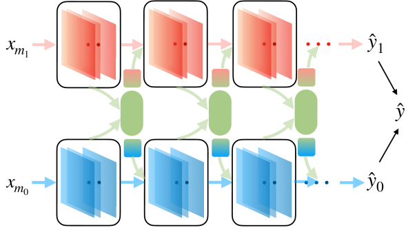
Figure 1: The multi-modal DNN with intermediate fusion that we study in this work. Blue and red blocks represent the two uni-modal networks, $\phi_{0}$ and $\phi_{1}$, learning from modalities $m_{0}$ and $m_{1}$. The fusion layers are marked with green, green-blue, and green-red. We denote the predictions from $\phi_{0}$ and $\phi_{1}$ by $\hat{y}_{0}$ and $\hat{y}_{1}$, and the average of the two by $\hat{y}$ which is the model’s prediction.

4 The Greedy Learner Hypothesis

In this section, we first derive conditional utilization rate to help explain the multi-modal DNN and to quantify its imbalance in modality utilization. Then we introduce the greedy learner hypothesis to explain challenges observed in training multi-modal DNNs.

4.1 Conditional Utilization Rate

In the multi-modal DNN shown in Figure 1, each uni-modal branch largely focuses on the associated input modality, and the fusion modules generate context information using all modalities, and feed the information to the uni-modal branches. Both $\hat{y}_{0}$ and $\hat{y}_{1}$ depend on information from both modalities. We derive $f_{0}$ and $f_{1}$ from $f$:

$$\hat{y}_{0}=f_{0}(\bm{x}_{m_{0}},\bm{x}_{m_{1}}),\quad\hat{y}_{1}=f_{1}(\bm{x}_{m_{0}},\bm{x}_{m_{1}}).$$ (5)

Let $\mathcal{D}^{\mathrm{train}}=\{\bm{x}^{i}\}_{i=1}^{n}$ and $h_{0}(\bm{x}^{i})$ and $h_{1}(\bm{x}^{i})$ denote the value of $h_{0}$ and $h_{1}$ when the model takes $\bm{x}^{i}$ as input. We compute the average of $h_{0}$ and $h_{1}$ over $\mathcal{D}^{\mathrm{train}}$:

$$\overline{h}_{0}=\frac{1}{n}\sum_{i=1}^{n}{h_{0}(\bm{x}^{i})},\quad\overline{h}_{1}=\frac{1}{n}\sum_{i=1}^{n}{h_{1}(\bm{x}^{i})}.$$ (6)

To estimate $f$’s reliance on each modality independently, we modify the operations introduced in §3 for each fusion module as below:

$$w_{0},*=g([h_{0},\,\overline{h}_{1}]),\quad*,w_{1}=g([\overline{h}_{0},\,h_{1}]).$$ (7)

With such modified operation in every fusion module in the multi-modal DNN, we cut off the road to share information between the uni-modal branches and let the output of each branch rely on a single modality. We derive $f^{\prime}_{0}$ and $f^{\prime}_{1}$ and denote their outputs by $\hat{y}^{\prime}_{0}$ and $\hat{y}^{\prime}_{1}$:

$$\hat{y}^{\prime}_{0}=f^{\prime}_{0}(\bm{x}_{m_{0}}),\quad\hat{y}^{\prime}_{1}=f^{\prime}_{1}(\bm{x}_{m_{1}}).$$ (8)

In summary, we derive four models from $f$ and compute the accuracy of each on $\mathcal{D}^{\mathrm{test}}$, denoted by $A(\cdot)$. We group the four accuracies into two pairs: $(A(f_{0}),A(f^{\prime}_{0}))$, and $(A(f_{1}),A(f^{\prime}_{1}))$.

We define the conditional utilization rates as bellow.

Definition 4.1 (Conditional utilization rate).

For a multi-modal DNN, $f$, taking two modalities $m_{0}$ and $m_{1}$ as inputs, its conditional utilization rates for $m_{0}$ and $m_{1}$ are defined as

$$\bm{u}(m_{0}|m_{1})=\frac{A(f_{1})-A(f^{\prime}_{1})}{A(f_{1})},$$ (9)

and

$$\bm{u}(m_{1}|m_{0})=\frac{A(f_{0})-A(f^{\prime}_{0})}{A(f_{0})}.$$ (10)

The conditional utilization rate is the relative change in accuracy between the two models within each pair. For example, $u(m_{0}|m_{1})$ measures the marginal contribution that $m_{0}$ has in increasing the accuracy of $\hat{y}_{1}$.

Let $\mathop{}\!\mathrm{d}_{\mathrm{util}}(f)$ denote the difference between conditional utilization rates: $\mathop{}\!\mathrm{d}_{\mathrm{util}}(f)=\bm{u}(m_{1}|m_{0})-\bm{u}(m_{0}|m_{1}).$ It is bounded between $-1$ and $1$. When $\mathop{}\!\mathrm{d}_{\mathrm{util}}(f)$ is close to $-1$ or $1$, the model benefits only from one of the modalities given the other but not vice versa. This implies that the model’s ability to predict $\hat{y}_{0}$ and $\hat{y}_{1}$ comes only from one of the modalities. Thus, if we observe high $|\mathop{}\!\mathrm{d}_{\mathrm{util}}(f)|$, we say that $f$ exhibits imbalance in utilization between modalities.

4.2 Multi-modal Learning Process is Greedy

We propose our hypothesis that builds on the following assumptions regarding multi-modal data, as well as observations previously made in the literature.

First, for most multi-modal learning tasks, both modalities are assumed to be predictive of the target. This can be expressed as $I(\bm{Y},\bm{X}_{m_{0}})>0$ and $I(\bm{Y},\bm{X}_{m_{1}})>0$, where $I$ denotes mutual information (Blum & Mitchell, 1998; Sridharan & Kakade, 2008). In order to minimize one of the modality-specific losses, e.g. $\mathrm{CE}(y,\hat{y}_{0})$, one can either update the parameters of the uni-modal branch taking $m_{0}$ as input, or the parameters of the fusion layers that pass information from $m_{1}$ to $\hat{y}_{0}$, or both.

Second, as shown in many tasks, different modalities have been said to be predictive of the target at different degrees. For example, it has been observed that when training DNNs on each modality separately, they usually do not reach the same level of performance (Wang et al., 2020b; Joze et al., 2020). In addition, multi-modal DNNs exhibit varying accuracy when trained on different subsets of modalities present for the task (Weng et al., 2021; Pérez-Rúa et al., 2019; Liu et al., 2018). Third, DNNs learn from different modalities at different speeds. This has been observed in both uni-modal DNNs and multi-modal DNNs (Wang et al., 2020a; Wu et al., 2020).

Now we formulate the greedy learner hypothesis to explain the behavior of multi-modal DNNs:

To characterize greediness of the multi-modal learning process, we need to repeat it several times. Every time, we sample a learning rate from a given range and initialize the network’ parameters randomly. Let $\mathbb{E}[\widehat{\mathop{}\!\mathrm{d}}_{\mathrm{util}}]$ denote the expectation of $\widehat{\mathop{}\!\mathrm{d}}_{\mathrm{util}}$ over the empirical distribution of the models obtained. The absolute value of $\mathbb{E}[\widehat{\mathop{}\!\mathrm{d}}_{\mathrm{util}}]$ is associated with the greediness of the process. The higher the $|\mathbb{E}[\widehat{\mathop{}\!\mathrm{d}}_{\mathrm{util}}]|$, the greedier the learning process.

To validate our hypothesis empirically, we conduct experiments on several multi-modal datasets using different network architectures (cf. §6.1). We show that the multi-modal learning process cannot avoid producing models that exhibit a high degree of imbalance in utilization between modalities. Their performance can be improved by using a less greedy algorithm which we will introduce in the next section.

5 Making Multi-modal Learning Less Greedy

We aim to make multi-modal learning less greedy by controlling the speed at which a multi-modal DNN learns to rely on each modality. In order to achieve this, we first define conditional learning speed to measure the speed at which the DNN learns from one modality. It serves as an efficient proxy for the conditional utilization rate of the corresponding modality, as shown empirically in §6.2 and §6.3. We then propose the balanced multi-modal learning algorithm, which controls the difference in conditional learning speed between modalities that the model exhibits during training.

5.1 Conditional Learning Speed

As demonstrated in §4.2, the imbalance in conditional utilization rates is a sign of the model exploiting the connection between the target and only one of the input modalities, ignoring cross-modal information. However, conditional utilization rates are designed to be measured after training is done and they are derived from the model’s accuracy achieved on the held-out test set. This makes conditional utilization rate not the best tool to use to monitor training at the real-time. We instead derive a proxy metric, called conditional learning speed, that captures relative learning speed between modalities during training.

Let us revisit the multi-modal DNN presented in Figure 1. We denote the parameters of uni-modal branches $\phi_{0}$ and $\phi_{1}$ by $\bm{\theta}_{0}$ and $\bm{\theta}_{1}$. Besides $\bm{\theta}_{0}$, we consider the parameters of the layers marked with green and green/blue, as important components of the function mapping $\bm{x}$ to $\hat{y}_{0}$ (i.e., $f_{0}$). These parameters are from the fusion modules and we refer to them as $\bm{\theta}^{\prime}_{0}$. Analogously, parameters in the layers marked with green and green/red are considered as important contributors to the function mapping $\bm{x}$ to $\hat{y}_{1}$ (i.e., $f_{1}$). We denote them by $\bm{\theta}^{\prime}_{1}$. In this way, we divide the model’s parameters into two pairs: $(\bm{\theta}_{0},\bm{\theta}^{\prime}_{0})$ and $(\bm{\theta}_{1},\bm{\theta}^{\prime}_{1})$.

We define the model’s conditional learning speed as follows.

Definition 5.1 (Conditional learning speed).

Given a multi-modal DNN, $f$, with two input modalities, $m_{0}$ and $m_{1}$, the conditional learning speeds of these modalities after $t$ training steps, are

$$\bm{s}(m_{1}|m_{0};t)=\log\frac{\sum_{i=1}^{t}\mu(\bm{\theta}^{\prime}_{0};i)}{\sum_{i=1}^{t}\mu(\bm{\theta}_{0};i)},$$ (11)

and

$$\bm{s}(m_{0}|m_{1};t)=\log\frac{\sum_{i=1}^{t}\mu(\bm{\theta}^{\prime}_{1};i)}{\sum_{i=1}^{t}\mu(\bm{\theta}_{1};i)},$$ (12)

where for any parameters $\bm{\theta}$, let $\bm{\theta}_{(i-1)}$ and $\bm{\theta}_{(i)}$ denote its value before and after the gradient descent step $i$; we have $\bm{G}=\frac{\partial{L}}{\partial{\bm{\theta}}}|_{\bm{\theta}_{(i-1)}}$; and $\mu(\bm{\theta};i)=||\bm{G}||^{2}_{2}/||\bm{\theta}_{(i)}||^{2}_{2}$ quantifies the change of $f$ that comes from updating $\bm{\theta}$ at the $i^{th}$ step, which is also interpreted as the effective update on $\bm{\theta}$.

This definition of $\mu(\bm{\theta};i)$ is inspired by the discussion on the effective update of parameters (Van Laarhoven, 2017; Zhang et al., 2019; Brock et al., 2021; Hoffer et al., 2018). When normalization techniques, such as batch normalization (Ioffe & Szegedy, 2015), are applied to the DNNs, the key property of the weight vector, $\bm{\theta}$, is its direction, i.e., $\bm{\theta}/||\bm{\theta}||^{2}_{2}$. Thus, we measure the update on $\bm{\theta}$ using the norm of its gradient normalized by its norm.

The conditional learning speed, $\bm{s}(m_{1}|m_{0};t)$, is the log-ratio between the learning speed of $\bm{\theta}^{\prime}_{0}$ and that of $\bm{\theta}_{0}$. Because $\bm{\theta}^{\prime}_{0}$ carries information from $m_{1}$ to $\hat{y}_{0}$ and information from $m_{0}$ to $\hat{y}_{0}$ is carried by $\bm{\theta}_{0}$, $\bm{s}(m_{1}|m_{0};t)$ reflects how fast the model learns from $m_{1}$ relative to $m_{0}$ after the first $t$ steps.

We compute the difference between $\bm{s}(m_{1}|m_{0};t)$ and $\bm{s}(m_{0}|m_{1};t)$ as: $\mathop{}\!\mathrm{d}_{\mathrm{speed}}(f;t)=\bm{s}(m_{1}|m_{0};t)-\bm{s}(m_{0}|m_{1};t)$ analogous to $\mathop{}\!\mathrm{d}_{\mathrm{util}}(f)$. For each model, we report $\mathop{}\!\mathrm{d}_{\mathrm{speed}}(f;T)$ as $\mathop{}\!\mathrm{d}_{\mathrm{speed}}(f)$ where the model takes $T$ steps until reaching the highest accuracy on $\mathcal{D}^{\mathrm{val}}$.

We anticipate that the conditional learning speed serves as a proxy for the conditional utilization rate. In §6.2 and §6.3, we show the distributions of $\widehat{\mathop{}\!\mathrm{d}}_{\mathrm{speed}}$ and $\widehat{\mathop{}\!\mathrm{d}}_{\mathrm{util}}$ side-by-side to validate this.

5.2 Balanced Multi-modal Learning

Since we assume $\mathop{}\!\mathrm{d}_{\mathrm{speed}}(f,t)$ is predictive of the imbalanced utilization between modalities, we can take advantage of $\mathop{}\!\mathrm{d}_{\mathrm{speed}}(f,t)$ to balance conditional utilization on-the-fly. In addition to training the network normally with both modalities, we accelerate the model to learn from either modality alternately to balance their conditional learning speeds. See Algorithm 1 for an overall description.

Algorithm 1 Balanced Multi-modal Learning

  Input: re-balancing window size $Q$, imbalance tolerance parameter $\alpha$, # epochs $N$, # updating steps per epoch $n$

  Initiate: $M_{\bm{\theta}_{0}},M_{\bm{\theta}^{\prime}_{0}},M_{\bm{\theta}_{1}},M_{\bm{\theta}^{\prime}_{1}}\leftarrow 0,0,0,0$; $q\leftarrow Q$

  for $i=1$ to $n$ do

     Take a regular step;

     $M_{\bm{\theta}_{0}}\leftarrow M_{\bm{\theta}_{0}}+\mu(\bm{\theta}_{0};i)$; $M_{\bm{\theta}^{\prime}_{0}}\leftarrow M_{\bm{\theta}^{\prime}_{0}}+\mu(\bm{\theta}^{\prime}_{0};i)$;

     $M_{\bm{\theta}_{1}}\leftarrow M_{\bm{\theta}_{1}}+\mu(\bm{\theta}_{1};i)$; $M_{\bm{\theta}^{\prime}_{1}}\leftarrow M_{\bm{\theta}_{1}}+\mu(\bm{\theta}^{\prime}_{1};i)$;

  end for

  for $i=1$ to $n\times N$ do

     if $q==Q$ then

        Take a regular step;

        $M_{\bm{\theta}_{0}}\leftarrow M_{\bm{\theta}_{0}}+\mu(\bm{\theta}_{0};i)$; $M_{\bm{\theta}^{\prime}_{0}}\leftarrow M_{\bm{\theta}^{\prime}_{0}}+\mu(\bm{\theta}^{\prime}_{0};i)$;

        $M_{\bm{\theta}_{1}}\leftarrow M_{\bm{\theta}_{1}}+\mu(\bm{\theta}_{1};i)$; $M_{\bm{\theta}^{\prime}_{1}}\leftarrow M_{\bm{\theta}_{1}}+\mu(\bm{\theta}^{\prime}_{1};i)$;

        $\mathop{}\!\mathrm{d}_{\mathrm{speed}}=\log(M_{\bm{\theta}^{\prime}_{0}}/M_{\bm{\theta}_{0}})-\log(M_{\bm{\theta}^{\prime}_{1}}/M_{\bm{\theta}_{1}})$;

        if $|\mathop{}\!\mathrm{d}_{\mathrm{speed}}|>\alpha$ then $q\leftarrow 1$;

     else

        $q\leftarrow q+1$

        Take a re-balancing step to accelerate learning from $m_{0}$ if $\mathop{}\!\mathrm{d}_{\mathrm{speed}}>0$ else from $m_{1}$;

     end if

  end for

We refer to the training steps at which we perform forward and backward passes normally as the regular steps. We introduce the re-balancing steps at which we update one of the uni-modal branches intentionally in order to accelerate the model to learn from its input modality.

In a re-balancing step where we aim to accelerate the model’s learning from $m_{0}$, in every fusion module in the network, we re-scale the feature maps $\bm{A}_{1}$ in the same way as in §3 but we re-scale $\bm{A}_{0}$ differently:

$$\tilde{\bm{A}_{0}} =2\times\sigma(\overline{w}_{0})\odot\bm{A}_{0}, \tilde{\bm{A}_{1}} =2\times\sigma(w_{1})\odot\bm{A}_{1},$$ (13)

where $\{\bm{x}^{i}\}_{i=1}^{n_{t}}$ are the $n_{t}$ samples used in the previous regular training steps; $w_{0}(\bm{x}^{i})$ denotes the activation when the model takes $\bm{x}^{i}$ as input; and $\overline{w}_{0}=1/n_{t}\sum_{i=1}^{n_{t}}w_{0}(\bm{x}^{i})$.

In a re-balancing step to accelerate learning from $m_{1}$, we apply the modification on $\bm{A}_{1}$ instead of $\bm{A}_{0}$:

$$\tilde{\bm{A}_{0}} =2\times\sigma(w_{0})\odot\bm{A}_{0}, \tilde{\bm{A}_{1}} =2\times\sigma(\overline{w}_{1})\odot\bm{A}_{1},$$ (14)

where $\overline{w}_{1}=1/n_{t}\sum_{i=1}^{n_{t}}w_{1}(\bm{x}^{i}).$

To warm-up the model, we perform only regular steps in the first epoch. Then we switch from regular steps to re-balancing steps if $|\mathop{}\!\mathrm{d}_{\mathrm{speed}}(t)|>\alpha$, where $\alpha$ is a hyperparameter, referred to as the imbalance tolerance parameter. Once it switches to re-balancing mode, we takes $Q$ re-balancing steps before returning to the regular mode. We refer to the hyperparameter $Q$ by the re-balancing window size.

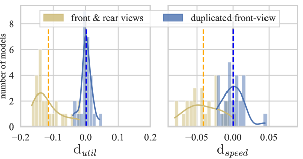
(a) ModelNet40

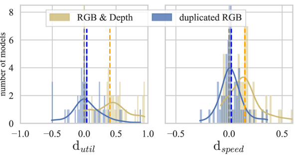
(b) NVGesture

Figure 2: Histograms and estimated density functions of $\widehat{\mathop{}\!\mathrm{d}}_{\mathrm{util}}$ and $\widehat{\mathop{}\!\mathrm{d}}_{\mathrm{speed}}$ of models trained using different modalities or duplicated single modality in (a) ModelNet40 or (b) NVGesture. We mark zero, $\mathbb{E}[\widehat{\mathop{}\!\mathrm{d}}_{\mathrm{util}}]$ and $\mathbb{E}[\widehat{\mathop{}\!\mathrm{d}}_{\mathrm{speed}}]$ with dashed lines. Many models have high $|\mathop{}\!\mathrm{d}_{\mathrm{util}}|$. We see $\widehat{\mathop{}\!\mathrm{d}}_{\mathrm{util}}$ is distributed asymmetrically around zero when using two different input modalities. When using two identical input modalities, it is distributed symmetrically around zero. We see $\widehat{\mathop{}\!\mathrm{d}}_{\mathrm{speed}}$ exhibits similar distributions as $\widehat{\mathop{}\!\mathrm{d}}_{\mathrm{util}}$.

6 Experiments and Results

6.1 Datasets, Tasks and Baselines

Colored-and-gray-MNIST (Kim et al., 2019) is a synthetic dataset based on MNIST (LeCun et al., 1998). In the training set of 60,000 examples, each example has two images, a gray-scale image and a monochromatic image, with color strongly correlated with its digit label. In the validation set of 10,000 examples, each example also has a gray-scale image and a corresponding monochromatic image, although with a low correlation between the color and its label. We consider the monochromatic image as the first modality $m_{0}$ and the gray-scale one as the second modality $m_{1}$. We use a neural network with four convolutional layers as the uni-modal branch and employ three MMTMs to connect them. The corresponding uni-modal DNNs trained on the monochromatic images and the gray-scale images achieve respective validation accuracies of 41% and 99%. We use this synthetic dataset mainly to demonstrate the proposed greedy learner hypothesis.

ModelNet40 is one of the Princeton ModelNet datasets (Wu et al., 2015) with 3D objects of 40 categories (9,483 training samples and 2,468 test samples). The task is to classify a 3D object based on the 2D views of its front and back (Su et al., 2015). Each example is a collection of 2D images (224$\times$224 pixels) of a 3D object. For the uni-modal branches, we use ResNet18 (He et al., 2016) and apply MMTMs in the three final residual blocks. The uni-modal DNNs achieve 89% and 88% accuracy when learning from the front view ($m_{0}$) and the rear view ($m_{1}$), respectively.

NVGesture (or NVIDIA Dynamic Hand Gesture Dataset (Molchanov et al., 2015)) consists of 1,532 video clips (1,050 training and 482 test ones) of hand gestures divided into 25 classes. We sample 20% of training examples as the validation set and use depth and RGB as the two modalities. We adopt the data preparation steps used in Joze et al. (2020) and use the I3D architecture (Carreira & Zisserman, 2017) as uni-modal branches and MMTMs as fusion modules in the six final inception modules. During training, we perform spatial augmentation on the video, including flipping and random cropping. During inference on the validation or test set, we perform center cropping on the video.

We provide examples of each dataset and details on data preprocessing in Appendix A.

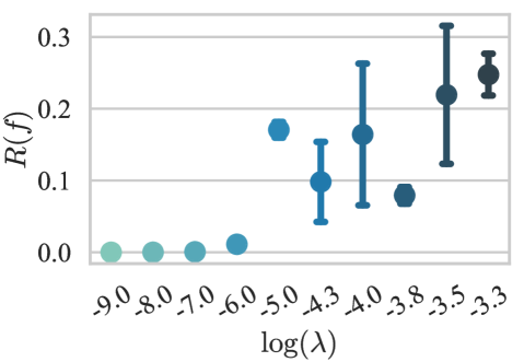
Figure 3: The mean and standard deviation of $R(f)$ for models trained with different weights ($\lambda$) on the L1 regularizer.. The larger the $\lambda$ is, the higher the $R(f)$ is, i.e., the sparser the model’s parameters are.

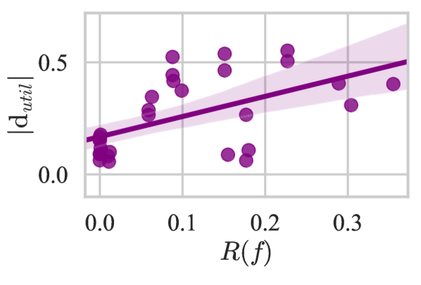
(a) $|\mathop{}\!\mathrm{d}_{\mathrm{util}}|$ vs. $R(f)$

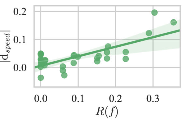
(b) $|\mathop{}\!\mathrm{d}_{\mathrm{speed}}|$ vs. $R(f)$

Figure 4: The observed $|\mathop{}\!\mathrm{d}_{\mathrm{util}}|$ and $|\mathop{}\!\mathrm{d}_{\mathrm{speed}}|$ for models trained with different weights ($\lambda$) on the L1 regularizer. In (a) and (b), we see both $|\mathop{}\!\mathrm{d}_{\mathrm{util}}|$ and $|\mathop{}\!\mathrm{d}_{\mathrm{speed}}|$ increases along $R(f)$. It indicates that the multi-modal learning process becomes greedier if we introduce stronger regularization.

6.2 Validating the Greedy Learner Hypothesis

In this section, we run the conventional multi-modal learning process on tasks with different input and output pairs to illustrate our hypothesis experimentally.

For each task introduced in §6.1, in addition to the original dataset, we construct a dataset with two identical input modalities by duplicating one of the modalities. For example, when using the colored-and-gray-MNIST dataset, we predict the digit class using two identical gray-scale images. We train multi-modal DNNs on these datasets as explained below for each task:

• Colored-and-gray-MNIST: we train multi-modal DNNs using SGD with a momentum coefficient of 0.9 and a batch size of 128. We sample 20 learning rates at random from the interval $[10^{-5},1]$ on a logarithmic scale. We train the model four times using each of the learning rates and random initialization of the parameters. In total, we train 80 models.

• ModelNet40: we use SGD without momentum and use a batch size of eight. We select nine learning rates from $10^{-3}$ to $1$ and train three copies of the model for each learning rate. This ends up with 27 models.

• NVGesture: we use a batch size of four, SGD with a momentum of 0.9, and uniformly sample 20 learning rates from the interval $[10^{-4}$, $10^{-1.5}]$ on a logarithmic scale. We train the model three times using each learning rate, resulting in 60 models in total.

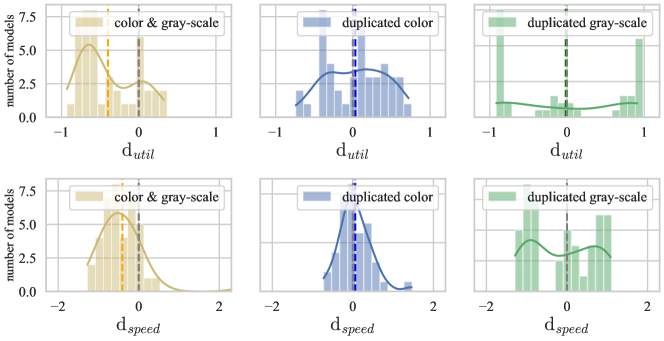
Figure 7: Histograms and estimated density functions of $\mathop{}\!\mathrm{d}_{\mathrm{util}}$ and $\mathop{}\!\mathrm{d}_{\mathrm{speed}}$ of models trained for colored-and-gray-MNIST, using monochromatic and gray-scale images as two modalities, using identical monochromatic images as two modalities and using identical gray-scale images as two modalities. Note that $\mathop{}\!\mathrm{d}_{\mathrm{speed}}$ is not bounded by 1 as $\mathop{}\!\mathrm{d}_{\mathrm{util}}$ is. Thus when learning from the two modalities is happening at very different paces, we can observe patterns shown in this study.

We present the results of the experiments on ModelNet40 and NVGesture in Figure 2 and on Colored-and-gray-MNIST in Figure 7 in Appendix B. We discuss three most interesting phenomena that we observe in the results.

First, many models have high $|\mathop{}\!\mathrm{d}_{\mathrm{util}}|$. This confirms that the multi-modal learning process encourages the model to rely on one modality and ignore the other one, which is consistent with our hypothesis. We make this observation across all tasks, confirming that the conventional multi-modal learning process is greedy regardless of network architectures and tasks.

Second, $\widehat{\mathop{}\!\mathrm{d}}_{\mathrm{util}}$ is distributed symmetrically around zero, and $\mathbb{E}[\widehat{\mathop{}\!\mathrm{d}}_{\mathrm{util}}]$ is approximately $0.0$, for all the experiments using two identical input modalities. On the other hand, if we use two distinct modalities, $\widehat{\mathop{}\!\mathrm{d}}_{\mathrm{util}}$ is distributed asymmetrically, and we observe $|\mathbb{E}[\widehat{\mathop{}\!\mathrm{d}}_{\mathrm{util}}]|$ of approximately 0.3, 0.1 and 0.4 for colored-and-gray-MNIST, ModelNet40 and NVGesture, respectively. We formalize the above observations as the following conjecture.

There exists an $\epsilon>0$, s.t. $|\mathbb{E}[\widehat{\mathop{}\!\mathrm{d}}_{\mathrm{util}}]|>\epsilon$, when modalities are different. Otherwise, $\widehat{\mathop{}\!\mathrm{d}}_{\mathrm{util}}$ is distributed symmetrically around zero and $\mathbb{E}[\widehat{\mathop{}\!\mathrm{d}}_{\mathrm{util}}]=0$.

Third, by observing conditional learning speed $\widehat{\mathop{}\!\mathrm{d}}_{\mathrm{speed}}$, we can draw the same conclusions. In fact, the distributions of $\widehat{\mathop{}\!\mathrm{d}}_{\mathrm{speed}}$ largely replicate the distributions of $\widehat{\mathop{}\!\mathrm{d}}_{\mathrm{util}}$. It validates our greedy learner hypothesis which attributes the imbalance in reliance on different modalities to the varying rate at which the learner learns from them. It moreover confirms $\mathop{}\!\mathrm{d}_{\mathrm{speed}}$ is an appropriate proxy to use to re-balance multi-modal learning.

Table 1: Test accuracy of best uni-modal DNNs and multi-modal DNNs trained using different strategies.

	Colored-and-gray-MNIST	ModelNet40	NVGesture-scratch	NVGesture-pretrained
uni-modal (best)	99.14$\pm$0.111	89.34$\pm$0.39	77.59$\pm$0.55	78.98$\pm$2.02
multi-modal (vanilla)	45.26$\pm$0.46	90.09$\pm$0.58	79.81$\pm$1.14	83.20$\pm$0.21
+ RUBi (Cadene et al., 2019)	44.79$\pm$0.62	90.45$\pm$0.58	79.95$\pm$0.12	81.60$\pm$1.28
+ random (proposed)	74.07$\pm$2.75	91.36$\pm$0.10	79.88$\pm$0.90	82.64$\pm$0.84
+ guided (proposed)	91.01$\pm$1.20	91.37$\pm$0.28	80.22$\pm$0.73	83.82$\pm$1.45

• The monochromatic image cannot help with the prediction and it is hard to avoid it hurting the ensemble performance. The uni-modal branch taking gray-scale image in the multi-modal DNNs (guided) achieves an accuracy of 99.16$\pm$0.14.

6.3 Strong Regularization Encourages Greediness

We also conjecture that regularization is a factor impacting the greediness of learning in multi-modal DNNs and strong regularization encourages greediness. We provide the following study to validate this.

We investigate L1 regularization’s impact on multi-modal DNNs. Precisely, we train the networks to optimize the loss $L^{\prime}=L+\lambda||\bm{\theta}||_{1}$, where $L$ is the classification loss in §3, $\bm{\theta}$ stands for all model parameters and $\lambda$ is the weight on the regularizer.

We measure the effect of $\lambda$ on the network $f$ by computing the fraction of its parameters smaller than $10^{-7}$. We denote this quantity by $R(f)$. Since L1 regularization encourages sparsity of the network’s parameters, as shown in Figure 4, the larger the $\lambda$, the higher the $R(f)$.

We conduct this study with ModelNet40, using the front and the rear views. We compute $|\mathop{}\!\mathrm{d}_{\mathrm{util}}(f)|$ for ten values of $\lambda$ from an interval $[10^{-9},10^{-3}]$. We use SGD without momentum, we set the learning rate to 0.1 and batch size to eight. Using each combination of hyperparameters, we repeat training for three times with random initialization and get three models.

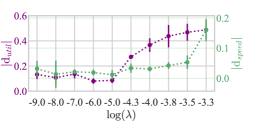
Figure 8: The observed $|\mathop{}\!\mathrm{d}_{\mathrm{util}}|$ and $|\mathop{}\!\mathrm{d}_{\mathrm{speed}}|$ for models trained with different weights ($\lambda$) on the L1 regularizer. We show $|\mathop{}\!\mathrm{d}_{\mathrm{util}}|$ and $|\mathop{}\!\mathrm{d}_{\mathrm{speed}}|$ as a function of $\log(\lambda)$. As we can see, when $\log(\lambda)\geq-5$, both $|\mathop{}\!\mathrm{d}_{\mathrm{util}}(f)|$ and $|\mathop{}\!\mathrm{d}_{\mathrm{speed}}|$ increases with $\lambda$ increasing, .

As shown in Figure 4, $|\mathop{}\!\mathrm{d}_{\mathrm{util}}(f)|$ is positively correlated with $R(f)$, and when $\lambda\geq 10^{-5}$, $|\mathop{}\!\mathrm{d}_{\mathrm{util}}(f)|$ increases significantly with $\lambda$ increasing, as shown in Figure 8 in Appendix B. In other words, the stronger the regularization is, the larger the imbalance in utilization between modalities we observe. We also find that $|\mathop{}\!\mathrm{d}_{\mathrm{speed}}|$ follows the same trend as $|\mathop{}\!\mathrm{d}_{\mathrm{util}}|$. Again, it supports our choice of using the conditional learning speed to predict the conditional utilization rate.

6.4 Balanced Multi-modal Learning

Besides the proposed training algorithm (cf. §5.2, referred to as guided), we introduce a variant of it, referred to as random: we perform regular steps in the first epoch, and afterwards, we let the model take a step that is randomly sampled from: regular step, re-balancing step on $m_{0}$, and re-balancing step on $m_{1}$. This algorithm is motivated by Modality Dropout (Neverova et al., 2015) but better suited to multi-modal DNNs with intermediate fusion. We consider it a stronger baseline that can also balance learning from inputs of different modalities.

Calibrated modality utilization

We train multi-modal DNNs as described in §6.2, using the guided, the random, and the conventional training algorithm (referred to as vanilla). For ModelNet40, we set the imbalance tolerance parameter $\alpha$ to 0.01 and the re-balancing window size $Q$ to 5. For NVGesture, we use $\alpha$ of 0.1 and $Q$ of 5. Results are shown in Figure 5. Models trained with the guided algorithm have lower $|\widehat{\mathop{}\!\mathrm{d}}_{\mathrm{util}}|$ compared to the vanilla algorithm. On NVGesture, we obtain $\mathbb{E}[\widehat{\mathop{}\!\mathrm{d}}_{\mathrm{util}}]$ of approximately 0.3 and 0.4 for models trained with the guided and the vanilla algorithm. On ModelNet40, we obtain $\mathbb{E}[\widehat{\mathop{}\!\mathrm{d}}_{\mathrm{util}}]$ of approximately -0.0, and -0.1 for models trained with the guided and the vanilla algorithm.

The random version of the proposed method also calibrates modality utilization effectively, giving $\mathbb{E}[\widehat{\mathop{}\!\mathrm{d}}_{\mathrm{util}}]$ of approximately 0.1 and -0.0 for models trained on NVGesture and ModelNet40. We will see in the next section that it helps less on generalization compared to the guided version.

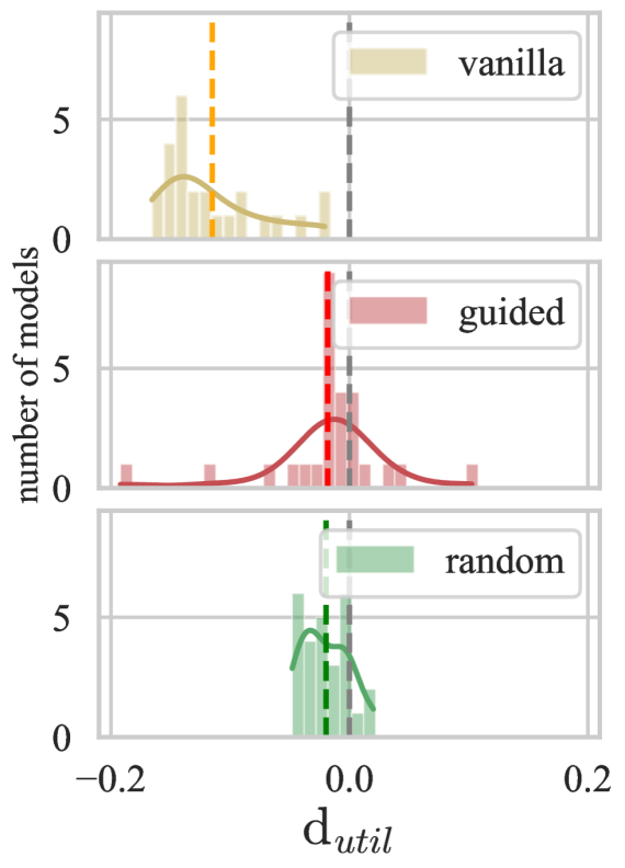
(a) ModelNet40

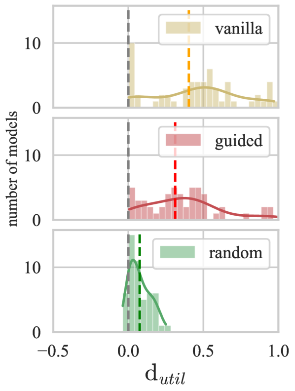
(b) NVGesture

Figure 5: Histograms and estimated density functions of $\widehat{\mathop{}\!\mathrm{d}}_{\mathrm{util}}$ of models trained using the vanilla, the guided and the random algorithm on (a) ModelNet40 and (b) NVGesture. We use dashed lines to mark zero and $\mathbb{E}[\widehat{\mathop{}\!\mathrm{d}}_{\mathrm{util}}]$ over the set of models trained with each of the algorithms. Both versions of the proposed algorithm is less greedy than the vanilla one.

Improved generalization performance

We compare the generalization ability of multi-modal DNNs trained by the baseline (vanila), the proposed methods (guided and random) and the RUBi learning strategy (Cadene et al., 2019). We chose RUBi as one of the baselines since it is model-agnostic and fusion-method-agnostic, and it is easy to adapt to different tasks. RUBi is designed to serve a similar purpose, that is, to encourage the model to learn from all modalities and has been shown to be helpful for VQA.

For each algorithm, we train each model three times with the same learning rate. We use 0.01, 0.1 and 0.01 as learning rate for Colored-and-gray-MNIST, ModelNet40 and NVGesture respectively. We use $\alpha$ of 0.1 for Colored-and-gray-MNIST and NVGesture and 0.01 for ModelNet40. We set $Q$ of 5 for all three datasets. For NVGesture, we add one experiment where we initialize the model with parameters pre-trained using the Kinetics dataset (Carreira & Zisserman, 2017) in addition to random initialization. We refer to this setting as “NVGesture-pretrained” and to the other one as “NVGesture-scratch”.

Besides the multi-modal DNNs trained using different strategies, we implement Squeeze-and-Excitation blocks (hu2018squeeze) to obtain uni-modal DNNs that are comparable to the multi-modal DNNs with MMTMs (Joze et al., 2020). We train uni-modal DNNs with each modality and present the best performance they achieve for each task. We report means and standard deviations of the models’ test accuracies in Table 1. The guided algorithm improves the models’ generalization performance over all other three methods in all four cases. RUBi does not show consistent improvement across tasks compared to the vanilla algorithm. We did not find this strategy as helpful as reported for VQA.

Our idea can be extended naturally to tasks with more than two modalities. The conditional learning speed of the $i^{th}$ modality can be derived using the weight norm and gradient norm of the $i^{th}$ uni-modal network’s parameters and the fusion module’s parameters impacting $\hat{y}_{i}$. The conditional utilization rate would be computed analogously to the bi-modal case, by passing the averaged feature maps of all other modalities to the fusion modules. We define $\mathop{}\!\mathrm{d}_{\mathrm{speed}}$ by the two most different conditional learning speeds and accelerate the learning of one modality per time. We experiment with three views in ModelNet40 and find that the guided algorithm outperforms the vanilla one as it improves the accuracy from $91.21\%$ to $92.45\%$.

In summary, we present that the greediness of the current training algorithm is an issue preventing multi-modal DNNs from achieving better performance. The proposed method can help to overcome this issue on multiple datasets.

7 Discussion

Our work demonstrates that the end-to-end trained multi-modal DNNs rely on one of the input modalities to make predictions while leaving the other modalities underutilized. For many multi-modal classification tasks, such as video classification, the harm of this behavior may not be as obvious as in VQA which strongly relies on cross-modal reasoning. However, the tools we propose in this work enable us to have a concrete look of what the model has learned, which has been a missing component in multi-modal learning systems. We validated our statements experimentally on three multi-modal datasets and illustrated that using the proposed algorithm to balance the models’ learning from different modalities enhances generalization. This result emphasizes that the adequate modality utilization is a desired property that a model should achieve in multi-modal learning. In addition to the previous discussion on this problem, our greedy learner hypothesis provides a complementary explanation and the methods inspired by it enrich the spectrum of available tools for multi-modal learning.

Appendix A Data Preparation

We used three datasets in the paper: Colored MNIST dataset (Kim et al., 2019), ModelNet40 dataset (Su et al., 2015) and NVGesture dataset (Molchanov et al., 2015), as illustrated in Figure 6.

For Colored MNIST and ModelNet40, we did not perform any extra data pre-processing steps on the original datasets.

For the NVGesture dataset, each video has a resolution of 240$\times$320 and a duration of 80 frames from action starting to ending. There are three videos with unmatched starting indices between RGB and depth. We adopt the starting frame indice of RGB for all modalities. We randomly select 64 consecutive frames from the videos in the dataset and if the video has less than 64 frames, we zero-pad on both sides of it to obtain 64 frames. Frames are resized as 256$\times$256 and are cropped into 224$\times$224 as inputs (we use static cropping where we crop from the same location across times and modalities).

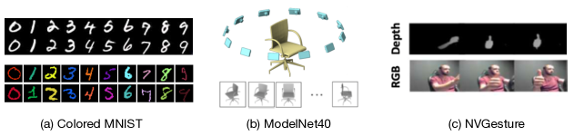
Figure 6: (a) The Colored MNIST dataset (Kim et al., 2019). We consider the monochromatic image, and the gray-scale image as the two input modalities (b) The ModelNet40 dataset (Su et al., 2015). The 2D representations are gray-scale images rendered from 12 different viewpoints of the object. (c)The NVGesture dataset (Molchanov et al., 2015). We use depth and RGB channels as the two modalities.

Appendix B Supplementary Figures

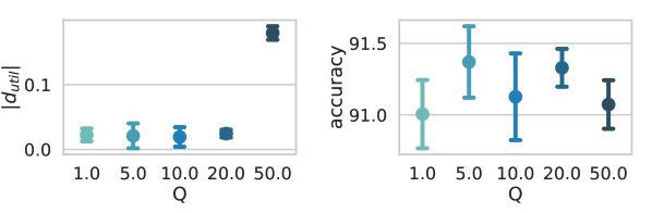
(a) We train models using $Q\in\{1,5,10,20,50\}$ and $\alpha=0.01$. Except $Q=50$, models trained using other values of $Q$ present relatively balanced conditional utilization rates between modalities (left panel). According to the models’ generalization performance (right panel), we choose $Q=5$ for the final experiment.

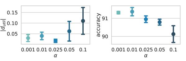
(b) We train models using $Q=5$ and $\alpha\in\{0.01,0.1,0.25,0.5,1\}\times\mathbb{E}[\widehat{\mathop{}\!\mathrm{d}}_{\mathrm{util}}]$, where $\mathbb{E}[\widehat{\mathop{}\!\mathrm{d}}_{\mathrm{util}}]=0.1$ as shown in §6.2. When setting $\alpha\leq 0.25\mathbb{E}[\widehat{\mathop{}\!\mathrm{d}}_{\mathrm{util}}]$, we can control $\mathop{}\!\mathrm{d}_{\mathrm{util}}$ effectively (left panel). We choose to use $\alpha=0.1\mathbb{E}[\widehat{\mathop{}\!\mathrm{d}}_{\mathrm{util}}]=0.01$ based on the models’ accuracy (right panel) for the final experiment.

Figure 9: Models’ behavior when using different values for the imbalance tolerance parameter $\alpha$ and the re-balancing window size $Q$ in the balanced multi-modal training algorithm. We use ModelNet40 (front and rear views) and fix the learning rate at 0.1 for the studies on both hyperparameters.

References

- Agrawal et al. (2016) Agrawal, A., Batra, D., and Parikh, D. Analyzing the behavior of visual question answering models. EMNLP, 2016.
- Agrawal et al. (2018) Agrawal, A., Batra, D., Parikh, D., and Kembhavi, A. Don’t just assume; look and answer: Overcoming priors for visual question answering. In CVPR, 2018.
- Anderson et al. (2018) Anderson, P., He, X., Buehler, C., Teney, D., Johnson, M., Gould, S., and Zhang, L. Bottom-up and top-down attention for image captioning and visual question answering. CVPR, 2018.
- Arnab et al. (2021) Arnab, A., Dehghani, M., Heigold, G., Sun, C., Lučić, M., and Schmid, C. Vivit: A video vision transformer. arXiv:2103.15691, 2021.
- Atrey et al. (2010) Atrey, P. K., Hossain, M. A., El Saddik, A., and Kankanhalli, M. S. Multimodal fusion for multimedia analysis: a survey. Multimedia Systems, 2010.
- Baltrušaitis et al. (2018) Baltrušaitis, T., Ahuja, C., and Morency, L.-P. Multimodal machine learning: A survey and taxonomy. IEEE Transactions on Pattern Analysis and Machine Intelligence, 2018.
- Blum & Mitchell (1998) Blum, A. and Mitchell, T. Combining labeled and unlabeled data with co-training. COLT, 1998.
- Brock et al. (2021) Brock, A., De, S., Smith, S. L., and Simonyan, K. High-performance large-scale image recognition without normalization. ICML, 2021.
- Cadene et al. (2019) Cadene, R., Dancette, C., Ben-Younes, H., Cord, M., and Parikh, D. Rubi: Reducing unimodal biases in visual question answering. NeurIPS, 2019.
- Cao et al. (2020) Cao, J., Gan, Z., Cheng, Y., Yu, L., Chen, Y.-C., and Liu, J. Behind the scene: Revealing the secrets of pre-trained vision-and-language models. ECCV, 2020.
- Carreira & Zisserman (2017) Carreira, J. and Zisserman, A. Quo vadis, action recognition? a new model and the kinetics dataset. CVPR, 2017.
- Gat et al. (2020) Gat, I., Schwartz, I., Schwing, A., and Hazan, T. Removing bias in multi-modal classifiers: Regularization by maximizing functional entropies. NeurIPS, 2020.
- Gat et al. (2021) Gat, I., Schwartz, I., and Schwing, A. Perceptual score: What data modalities does your model perceive? NeurIPS, 34, 2021.
- Goyal et al. (2017) Goyal, Y., Khot, T., Summers-Stay, D., Batra, D., and Parikh, D. Making the V in VQA matter: Elevating the role of image understanding in Visual Question Answering. CVPR, 2017.
- Han et al. (2021a) Han, X., Wang, S., Su, C., Huang, Q., and Tian, Q. Greedy gradient ensemble for robust visual question answering. ICCV, 2021a.
- Han et al. (2021b) Han, Z., Zhang, C., Fu, H., and Zhou, J. T. Trusted multi-view classification. ICLR, 2021b.
- He et al. (2016) He, K., Zhang, X., Ren, S., and Sun, J. Deep residual learning for image recognition. CVPR, 2016.
- Hessel & Lee (2020) Hessel, J. and Lee, L. Does my multimodal model learn cross-modal interactions? it’s harder to tell than you might think! EMNLP, 2020.
- Hoffer et al. (2018) Hoffer, E., Banner, R., Golan, I., and Soudry, D. Norm matters: efficient and accurate normalization schemes in deep networks. NeurIPS, 2018.
- Ioffe & Szegedy (2015) Ioffe, S. and Szegedy, C. Batch normalization: Accelerating deep network training by reducing internal covariate shift. ICML, 2015.
- Jabri et al. (2016) Jabri, A., Joulin, A., and Van Der Maaten, L. Revisiting visual question answering baselines. ECCV, 2016.
- Joze et al. (2020) Joze, H. R. V., Shaban, A., Iuzzolino, M. L., and Koishida, K. Mmtm: multimodal transfer module for cnn fusion. CVPR, 2020.
- Kim et al. (2019) Kim, B., Kim, H., Kim, K., Kim, S., and Kim, J. Learning not to learn: Training deep neural networks with biased data. CVPR, 2019.
- Lao et al. (2021) Lao, M., Guo, Y., Liu, Y., Chen, W., Pu, N., and Lew, M. S. From superficial to deep: Language bias driven curriculum learning for visual question answering. In Proceedings of the 29th ACM International Conference on Multimedia, pp. 3370–3379, 2021.
- Lazaridou et al. (2015) Lazaridou, A., Baroni, M., et al. Combining language and vision with a multimodal skip-gram model. HLT-NAACL, 2015.
- LeCun et al. (1998) LeCun, Y., Bottou, L., Bengio, Y., and Haffner, P. Gradient-based learning applied to document recognition. Proceedings of the IEEE, 1998.
- Li et al. (2020) Li, L., Gan, Z., and Liu, J. A closer look at the robustness of vision-and-language pre-trained models. arXiv:2012.08673, 2020.
- Liu et al. (2018) Liu, K., Li, Y., Xu, N., and Natarajan, P. Learn to combine modalities in multimodal deep learning. arXiv:1805.11730, 2018.
- Molchanov et al. (2015) Molchanov, P., Gupta, S., Kim, K., and Kautz, J. Hand gesture recognition with 3d convolutional neural networks. CVPR, 2015.
- Nair & Hinton (2010) Nair, V. and Hinton, G. E. Rectified linear units improve restricted boltzmann machines. In ICML, 2010.
- Neverova et al. (2015) Neverova, N., Wolf, C., Taylor, G., and Nebout, F. Moddrop: Adaptive multi-modal gesture recognition. IEEE Transactions on Pattern Analysis and Machine Intelligence, 2015.
- Ngiam et al. (2011) Ngiam, J., Khosla, A., Kim, M., Nam, J., Lee, H., and Ng, A. Y. Multimodal deep learning. ICML, 2011.
- Perez et al. (2018) Perez, E., Strub, F., De Vries, H., Dumoulin, V., and Courville, A. Film: Visual reasoning with a general conditioning layer. AAAI, 2018.
- Pérez-Rúa et al. (2019) Pérez-Rúa, J.-M., Vielzeuf, V., Pateux, S., Baccouche, M., and Jurie, F. Mfas: Multimodal fusion architecture search. CVPR, 2019.
- Sridharan & Kakade (2008) Sridharan, K. and Kakade, S. M. An information theoretic framework for multi-view learning. COLT, 2008.
- Su et al. (2015) Su, H., Maji, S., Kalogerakis, E., and Learned-Miller, E. G. Multi-view convolutional neural networks for 3d shape recognition. ICCV, 2015.
- Sun et al. (2021) Sun, Y., Mai, S., and Hu, H. Learning to balance the learning rates between various modalities via adaptive tracking factor. IEEE Signal Processing Letters, 2021.
- Tran et al. (2015) Tran, D., Bourdev, L., Fergus, R., Torresani, L., and Paluri, M. Learning spatiotemporal features with 3d convolutional networks. ICCV, 2015.
- Van Laarhoven (2017) Van Laarhoven, T. L2 regularization versus batch and weight normalization. arXiv:1706.05350, 2017.
- Wang et al. (2020a) Wang, W., Tran, D., and Feiszli, M. What makes training multi-modal classification networks hard? CVPR, 2020a.
- Wang et al. (2020b) Wang, Y., Huang, W., Sun, F., Xu, T., Rong, Y., and Huang, J. Deep multimodal fusion by channel exchanging. NeurIPS, 2020b.
- Weng et al. (2021) Weng, Z., Wu, Z., Li, H., and Jiang, Y.-G. Hms: Hierarchical modality selectionfor efficient video recognition. arXiv:2104.09760, 2021.
- Winterbottom et al. (2020) Winterbottom, T., Xiao, S., McLean, A., and Moubayed, N. A. On modality bias in the tvqa dataset. BMVC, 2020.
- Wu et al. (2020) Wu, N., Jastrzębski, S., Park, J., Moy, L., Cho, K., and Geras, K. J. Improving the ability of deep networks to use information from multiple views in breast cancer screening. MIDL, 2020.
- Wu et al. (2015) Wu, Z., Song, S., Khosla, A., Yu, F., Zhang, L., Tang, X., and Xiao, J. 3d shapenets: A deep representation for volumetric shapes. CVPR, 2015.
- Zhang et al. (2019) Zhang, G., Wang, C., Xu, B., and Grosse, R. Three mechanisms of weight decay regularization. ICLR, 2019.